Dual Advancement of Representation Learning and Clustering for Sparse and Noisy Images

Abstract.

Sparse and noisy images (SNIs), like those in spatial gene expression data, pose significant challenges for effective representation learning and clustering, which are essential for thorough data analysis and interpretation. In response to these challenges, we propose Dual Advancement of Representation Learning and Clustering (DARLC), an innovative framework that leverages contrastive learning to enhance the representations derived from masked image modeling. Simultaneously, DARLC integrates cluster assignments in a cohesive, end-to-end approach. This integrated clustering strategy addresses the “class collision problem” inherent in contrastive learning, thus improving the quality of the resulting representations. To generate more plausible positive views for contrastive learning, we employ a graph attention network-based technique that produces denoised images as augmented data. As such, our framework offers a comprehensive approach that improves the learning of representations by enhancing their local perceptibility, distinctiveness, and the understanding of relational semantics. Furthermore, we utilize a Student’s t mixture model to achieve more robust and adaptable clustering of SNIs. Extensive experiments, conducted across 12 different types of datasets consisting of SNIs, demonstrate that DARLC surpasses the state-of-the-art methods in both image clustering and generating image representations that accurately capture gene interactions. Code is available at https://github.com/zipging/DARLC.

1. Introduction

Sparse and noisy images (SNIs), commonly encountered in specialized fields like biomedical sciences, astronomy, and microscopy  (Zhu et al., 2021; Sloka, 2023; Wang et al., 2023), are characterized by extensive uninformative regions (e.g., voids or background areas), considerable image noise, and severely fragmented visual patterns. These characteristics significantly increase the complexity in analysis and interpretation. A prime example is spatial gene expression Pattern (SGEP) images generated through spatial transcriptomics (ST) technology (Ståhl et al., 2016). As illustrated in Figure 1, the high levels of sparsity and noise of an SGEP image complicate the discerning of its underlying major gene expression pattern.

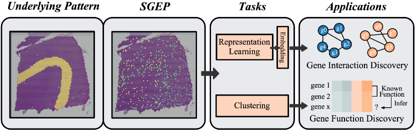
Figure 1. An example of sparse and noisy SGEP image is displayed in the second panel to the left. The gene expression levels across space are represented by pixel brightness, while void expression areas are displayed in purple. The first panel showcases the regions (cortical layer V) where the gene is significantly expressed, namely the major gene expression pattern. The right two panels illustrate the tasks and applications that utilize SGEP images.

Image clustering can group unlabelled images into distinct clusters, facilitating the exploration of image-implied semantics or functions. For example, clustering SGEP images offers a cost-effective means to identify groups of cofunctional genes and infer gene functions (Song et al., 2022). To obtain informative clustering results, it is essential to learn meaningful image representations, for which self-supervised learning (SSL) is the predominant approach in general scenarios. These include contrastive learning (CL) methods, exemplified by MoCo (He et al., 2020), and masked image modeling (MIM) such as MAE (He et al., 2022). These methods offer distinct learning perspectives: MIM methods tend to learn local context-aware, holistic features for reconstruction tasks (He et al., 2022), while CL methods focus on learning instance-wise discriminative features (Huang et al., 2023). Acknowledging the synergistic advantages of these methodologies, some researchers are endeavoring to utilize CL to refine the representations acquired through MIM (Zhou et al., 2021; Huang et al., 2023). Moreover, many efforts (Ren et al., 2022; Xie et al., 2016; Li et al., 2021a) are directed towards guiding the process of learning representations through clustering tasks. This is achieved by jointly learning representations and executing clustering in an integrated and end-to-end manner, yielding image representations that are well-suited for clustering tasks.

However, for SNIs, both representation learning and clustering present significant challenges. Firstly, the widespread presence of uninformative voids or background areas, along with elevated noise levels and extremely fragmented visual patterns, substantially impedes the extraction of semantically meaningful visual features. This challenge has been highlighted in prior studies (Lu et al., 2021) and is further corroborated by our experiments (see Supplementary Table 1). Secondly, the inherent random noise across pixels induces considerable variability in visual patterns, even among images of the same category (Song et al., 2022), exposing clustering algorithms to a high overfitting risk (Askari, 2021).

Inspired by the aforementioned works, in order to better analyze SNIs, we propose a novel and unified framework, named Dual Advancement of Representation Learning and Clustering (DARLC). This framework not only leverages CL to boost the representation learned by MIM but also jointly learns cluster assignments in a self-paced and end-to-end manner, further refining the representation. Nonetheless, our experiments (see Supplementary Table 2) showcase that conventional data augmentation techniques (e.g., cropping and rotating) are ineffective for SNIs, as the augmented images often contain substantial void regions and noise, hampering the extraction of informative visual features. To overcome this limitation, we introduce a data augmentation method based on a graph attention network (GAT) (Velickovic et al., 2018; Dong and Zhang, 2022) that aggregates information from neighboring pixels to enhance visual patterns, generating smoothed images that act as more plausible positive views so as to improve the effectiveness of contrastive learning.

Additionally, we observed that the clustering algorithms used in many deep clustering methods are either sensitive to outliers, as demonstrated by the Gaussian mixture model (GMM) in DAGMM (Zong et al., 2018) and manifold clustering in EDESC (Cai et al., 2022), or lack the flexibility to different data distributions, such as the inflexible Cauchy kernel-based method in DEC  (Xie et al., 2016). In response, DARLC employs a specialized nonlinear projection head to normalize image embeddings, aligning them more closely with a t-distribution. This is followed by modeling with a Student’s t mixture model (SMM) for soft clustering. SMM provides a more robust solution by down-weighing extreme values and is more adaptable by altering the degrees of freedom, making it particularly suitable for clustering in the context of SNIs. Furthermore, the clustering loss in DARLC also serves to regularize CL, alleviating the “class collision problem” that stems from false negative pairs in CL (Cai et al., 2020). Unlike existing regularized CL methods (Denize et al., 2023; Zheng et al., 2021; Li et al., 2021b), which directly integrate clustering into the CL throughout training, this clustering follows the “warm-up” representation learning, significantly expediting training convergence and enhancing clustering accuracy, as demonstrated in our ablation study. All these features collectively contribute to the finding that DARLC-generated image representations not only enhance clustering performance but also exhibit improvements in other semantic distance-based tasks, such as the discovery of functionally interactive genes. In summary, our main contributions are:

• We propose DARLC, a novel unified framework for dual advancement of representation learning and clustering for SNIs. DARLC marks the first endeavor in integrating contrastive learning, MIM and deep clustering into a cohesive process for representation learning. The resultant representations enhance image clustering performance and benefit other semantic distance-based tasks.

• DARLC has developed a data augmentation method more suitable for SNIs, using a GAT to generate smoothed images as plausible positive views for CL.

• An SMM-based method is designed to cluster SNIs in a more robust and adaptable manner. Additional features of this clustering method include a novel Laplacian loss for guiding the initial phase of clustering, and a differentiable cross-entropy hinge loss for controlling cluster sizes. This clustering also addresses the class collision problem by pulling close related instances.

• Extensive experiments have been conducted across 12 SNIs datasets. Our results show that DARLC surpasses the state-of-the-art (SOTA) methods in both image clustering and generating image representations that can be effectively applied to specific downstream tasks.

2. Related Works

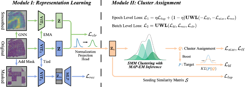
Figure 2. The framework of DARLC consists of two components: the representation learning and the deep clustering. The representation learning component integrates MIM and CL to generate image embeddings, which are then normalized through a non-linear projection head. Normalized representations are modeled by an SMM to derive their soft cluster assignments, which are used to construct various loss functions. With these loss functions, the two components are jointly optimized in a self-paced and end-to-end manner.

2.1. Self-supervised Representation Learning for Images

Most related SSL studies include CL and MIM methods. In CL, an input instance forms positive pairs with its augmented views, while forms negative pairs with other instances. Paradigmatic CL methods aim to learn instance discriminative representations by maximizing the similarity between positive pairs while minimizing it between negative pairs in a latent space (Chen et al., 2020; He et al., 2020). To address the class collision problem due to false negative samples, several studies (Li et al., 2021b; Denize et al., 2023; Zheng et al., 2021) regularize CL with clustering, while others (Grill et al., 2020; Caron et al., 2020, 2021; Chen and He, 2021) bypass the using of negative samples altogether. In contrast, MIM methods focus on learning local context-aware features by restoring raw pixel values from masked image patches (He et al., 2022; Gao et al., 2022; Xie et al., 2022; Bao et al., 2021). Several researchers are realizing the advantages of integrating these methodologies and endeavoring to utilize CL to refine MIM-generated representations (Xie et al., 2022; Huang et al., 2023). For instance, iBOT (Zhou et al., 2021) contrasts between the reconstructed tokens of masked and unmasked image patches. Yet, to the best of our knowledge, DARLC is the first method that learns image representations from all aspects of discriminability, local perceptability, and relational semantic structures.

2.2. Deep Image Clustering.

Related deep image clustering studies include deep autoencoder-based methods (Ren et al., 2022), which couple representation learning with deep embedded clustering in an end-to-end manner, as exemplified by methods like DEC (Xie et al., 2016; Li et al., 2018; Guo et al., 2017). Subsequent improvements to DEC focus on strategies like overweighing reliable samples (e.g., IDCEC  (Lu et al., 2022) ), and replacing Euclidean distance-based clustering with deep subspace clustering (e.g., EDESC (Cai et al., 2022)) or GMM-based clustering (Wang and Jiang, 2021; Zong et al., 2018). Recent studies, including CC (Li et al., 2021a), DCP (Lin et al., 2022), CVCL (Chen et al., 2023), and CCES (Yin et al., 2023), directly integrate CL into the clustering process by contrasting at both instance and cluster levels across views, generating a soft cluster assignment matrix as deep embeddings for iterative refinement. Compared to these methods, DARLC offers a more comprehensive and potent mechanism for learning deep embeddings, a more robust and adaptable clustering algorithm, and a warm-up representation learning phase for accelerating clustering convergence.

3. Methodology

3.1. Overview

The framework of DARLC, as illustrated in Figure 2 and Algorithm 1, comprises two modules: a self-supervised representation learning and a deep clustering. The self-supervised representation learning module unifies CL and MIM, encompassing three encoders: an online encoder and a target momentum encoder for the contrastive branch, and a masked encoder for the MIM branch. All three encoders adopt the identical vision transformer (ViT) (Dosovitskiy et al., 2020) architecture, with shared parameters between the online encoder and masked encoder. The parameters of the target momentum encoder are updated using exponential moving average (EMA), as suggested by BYOL (Grill et al., 2020). The initial phase of the unified representation learning involves a warm-up pretraining to generate preliminary embeddings, which are then normalized by a nonlinear projection head. This normalization aligns the embeddings more closely with t-distributions, setting the stage for subsequent t-distribution-based clustering. The deep clustering module utilizes a SMM to cluster the normalized embeddings, generating soft cluster assignment scores involved in the calculation of various loss functions. There are two types of loss functions: $\mathcal{L}_{1}$, an epoch-level loss function for maximizing the empirical likelihood of observed instances, and $\mathcal{L}_{2}$, a batch-level loss function for discriminatively boosted clustering optimization (Xie et al., 2016). The two loss functions work in tandem, enabling the joint refinement of image embeddings and cluster assignments in a self-paced and end-to-end manner.

Algorithm 1 Algorithm for Dual Advancement of Representations Learning and Clustering (DARLC).

1:Images $\mathcal{X}\in\mathbb{R}^{N\times C\times H\times W}$; Seeding similarity matrix $\mathcal{S}\in\mathbb{R}^{N\times N}$; Denoise GAT $\mathcal{G}$; Maximum epochs $E_{max}$; Number of images N; Number of clusters K.

2:Parametes of $\cdot$ are denoted as $\Pi(\cdot)$; MIM branch $\mathcal{M}$; CL branch $\mathcal{C}$; Projection head $\mathcal{H}$; UWL (Uncertain Weight Loss function); EMA (Exponential Moving Average function).

3:Representations $Z\in\mathbb{R}^{N\times D}$; Soft clustering $Q\in\mathbb{R}^{N\times K}$.

4:Compute smoothed image $\bar{\mathcal{X}}$ by Eq. (5).

5:while $epoch<E_{max}$ do

6:     for $\mathbf{X}_{b},\overline{\mathbf{X}}_{b}$ in $\mathcal{X},\hat{{\mathcal{X}}}$ do

7:         Compute $\widehat{\mathbf{X}}_{b}$ by Eq. (6) $\to\mathcal{L}_{rec}(\mathbf{X}_{b},\widehat{\mathbf{X}}_{b})$ by Eq. (7).

8:         Compute $\mathbf{e}_{b}$, $\overline{\mathbf{e}}_{b}$ by Eq. (9) $\to\mathcal{L}_{clr}(\mathbf{e}_{b},\overline{\mathbf{e}}_{b})$ by Eq. (3.2.2).

9:         $\mathcal{L}_{ssl}=\mathbf{UWL}(\mathcal{L}_{rec},\mathcal{L}_{clr})$.

10:         Update $\Pi(\mathcal{M})$ using $\mathcal{L}_{ssl}$.

11:         Update $\Pi(\mathcal{C})$ with $\mathbf{EMA}(\Pi(\mathcal{M}))$.

12:     end for

13:end while

14:while (not converged) & ($epoch<E_{max}$) do

15:     Compute $\widehat{\mathcal{X}}$ by Eq. (6) $\to\mathcal{L}_{rec}(\mathcal{X},\widehat{\mathcal{X}})$ by Eq. (7).

16:     Compute $\mathbf{Z}$ by Eqs. (9), (12) $\to\mathcal{L}_{\ell ap}(\mathbf{Z},\mathcal{S})$ by Eq. (17).

17:     SMM parameters inference using MAP-EM $\to\Theta$.

18:     $Q=\text{SMM}(\mathbf{Z}|\Theta)$ $\to\mathcal{L}_{size}(Q),\mathcal{L}_{\ell\ell}(Q)$ by Eqs. (20), (18).

19:     $\mathcal{L}_{1}=\eta\mathcal{L}_{\ell ap}+(1-\eta)\mathbf{UWL}(-\mathcal{L}_{\ell\ell},-\mathcal{L}_{size},\mathcal{L}_{rec})$.

20:     Update $\Pi(\mathcal{M}),\Pi(\mathcal{C}),\Pi(\mathcal{H})$ using $\mathcal{L}_{1}$.

21:     for $\mathbf{X}_{b},\overline{\mathbf{X}}_{b}$ in $\mathcal{X},\overline{{\mathcal{X}}}$ do

22:         Compute $P$ by Eq. (22) $\to\mathcal{L}_{kl}(P,Q)$ by Eq. (21).

23:         Compute $\widehat{\mathbf{X}}_{b}$ by Eq. (6) $\to\mathcal{L}_{rec}(\mathbf{X}_{b},\widehat{\mathbf{X}}_{b})$ by Eq. (7).

24:         Compute $\mathbf{e}_{b}$, $\overline{\mathbf{e}}_{b}$ by Eq. (9) $\to\mathcal{L}_{clr}(\mathbf{e}_{b},\overline{\mathbf{e}}_{b})$ by Eq. (3.2.2).

25:         $\mathcal{L}_{2}=\mathbf{UWL}(\mathcal{L}_{kl},\mathcal{L}_{rec},\mathcal{L}_{clr})$.

26:         Update $\Theta$ and $\Pi(\mathcal{M}),\Pi(\mathcal{C}),\Pi(\mathcal{H})$ using $\mathcal{L}_{2}$.

27:     end for

28:end while

29: return $\mathbf{Z},Q$

3.2. Unified Self-supervised Representation Learning (Module I)

3.2.1. Denoising-based Data Augmentation.

We train a graph attention autoencoder $\mathcal{G}$ to generate smoothed images, serving as augmented positive instances (Velickovic et al., 2018; Dong and Zhang, 2022). Initially, for each image, we construct an undirected and unweighted graph by treating pixels as nodes connected to their k-nearest neighbors. Specifically, for a given image $\mathbf{X}\in\mathbb{R}^{C\times H\times W}$, where $C$ is the number of channels, $H$ and $W$ are the height and width of the image, respectively. Let $N_{pix}=H\times W$ denote the number of pixels, $\mathbf{v}_{\iota}\in\mathbb{R}^{C}$ denote the pixel vector at location $\iota$, $\forall\iota\in\{1,2,...,N_{pix}\}$. The encoder in $\mathcal{G}$ comprises $L$ layers. For each layer $t\in\{1,2,...L-1\}$, with the initial value $\mathbf{h}_{\iota}^{(0)}=\mathbf{v}_{\iota}$, the output $\mathbf{h}_{\iota}^{(t)}\in\mathbb{R}^{d_{p}}$ is calculated as follows:

(1) $$\mathbf{h}_{\iota}^{(t)}=Leaky ReLU(\sum_{\nu\in S_{\iota}}\mathbf{att}_{\iota\nu}(\mathbf{W}^{(t)}\mathbf{h}_{\nu}^{(t-1)})),$$

where $\mathbf{W}^{(t)}$ represents the trainable weights of the $t$-th autoencoder layer, $S_{\iota}$ the set of node $\iota$’s neighbors within a pre-specified radius $r$. The attention score, $\mathbf{att}_{\iota\nu}$, between nodes $\iota$ and $\nu$ are computed as follows:

(2) $$\alpha_{\iota\nu}^{(t)}=\mathbf{w}_{att}^{(t)}LeakyReLU(\mathbf{W}^{(t)}[\mathbf{h}_{\iota}^{(t-1)})||\mathbf{h}_{\nu}^{(t-1)}]),$$

(3) $$\mathbf{att}_{\iota\nu}^{(t)}=\frac{\mathrm{exp}(\alpha_{\iota\nu}^{(t)})}{\sum_{\iota\in S_{\iota}}\mathrm{exp}(\alpha_{\iota\nu}^{(t)})},$$

where $\mathbf{w}_{att}^{(t)}$ represents the trainable attention weights. The decoder of $\mathcal{G}$ mirrors the encoder with tied weights. The total loss function is defined as:

(4) $$L_{denoise}=\sum_{\iota=1}^{N_{pix}}\|\mathbf{v}_{\iota}-\widetilde{\mathbf{h}}_{\iota}^{(0)}\|_{2},$$

where $\widetilde{\mathbf{h}}_{\iota}^{(0)}$ denotes the reconstructed $\mathbf{v}_{\iota}$ output by the decoder. Once trained, $\mathcal{G}$ is applied to any given image $\mathbf{X}_{i}$, to generate a smoothed image $\overline{\mathbf{X}}_{i}$ for a given image $\mathbf{X}_{i}$ as:

(5) $$\overline{\mathbf{X}}_{i}=\mathcal{G}(\mathbf{X}_{i},\textbf{W},w_{att})$$

3.2.2. Unified Self-supervised Image Representation Learning.

This SSL model encompasses two branches: a MIM branch $\mathcal{M}$ and a contrastive branch $\mathcal{C}$. $\mathcal{M}$ is an adapted version of MAE, specifically designed for generating image patch embeddings in the context of SNIs. In this adaption, the standard MAE encoder is replaced with a lightweight ViT encoder, denoted as $\mathcal{M}_{E}$, with four transformer blocks, four attention heads, and a higher masking ratio (80%). Meanwhile, the original transformer-based MAE decoder, is substituted with a fully-connected linear decoder $\mathcal{M}_{D}$. For any given image $\mathbf{X}_{i}$, the regenrated image $\widehat{\mathbf{X}}_{i}$ is as follows:

(6) $$\mathbf{\widehat{X}}_{i}=\mathcal{M}_{D}(\mathcal{M}_{E}(\mathbf{X}_{i},\,\mathbf{W}_{E}),\mathbf{W}_{D})$$

The MIM branch loss for the current batch are:

(7) $$\mathcal{L}_{rec}=\frac{1}{N_{b}}\sum_{i=1}^{N_{b}}\frac{1}{N_{masked}}\sum_{j\in S_{masked}}(\mathbf{p}_{i,j}-\widehat{\mathbf{p}}_{i,j})^{T}(\mathbf{p}_{i,j}-\widehat{\mathbf{p}}_{i,j}),$$

where $N_{b}$ is the batch size, $\mathbf{W}_{E}$ and $\mathbf{W}_{D}$ represent the parameters of the encoder and decoder, respectively. $N_{masked}$ denotes the number of masked patches, $S_{masked}$ the set of masked patches. $\mathbf{p}_{i,j}$ and $\widehat{\mathbf{p}}_{i,j}$ represent the original and regenerated $j$-th image patch of $\mathbf{X}_{i}$, respectively.

For the contrastive branch $\mathcal{C}$, the $N_{b}$ raw images form positive pairs with their respective smoothed images, and negative pairs with the other $2N_{b}-2$ images in the same batch. $\mathcal{C}$ is structured around a pseudo-siamese network with two encoders: an online encoder $\mathcal{C}_{O}$ and a target momentum encoder $\mathcal{C}_{T}$ . Both encoders share the identical network architecture as $\mathcal{P}_{E}$, with $\mathcal{C}_{O}$ and $\mathcal{P}_{E}$ having tied parameters. The parameters of $\mathcal{C}_{T}$ are updated using EMA. Concretely, let $\widetilde{\mathbf{W}}_{E}$ and $\overline{\mathbf{W}}_{E}$ denote the parameters of the $\mathcal{C}_{O}$ and $\mathcal{C}_{T}$, respectively. Then we have:

(8) $$\widetilde{\mathbf{W}}_{E}=\mathbf{W}_{E},\,\overline{\mathbf{W}}_{E}=m\overline{\mathbf{W}}_{E}+(1-m)\widetilde{\mathbf{W}}_{E}$$

Here, $m$ represents the momentum, fixed at 0.999. For each image $\mathbf{X}_{i}$ and its augmented counterpart $\overline{\mathbf{X}}_{i}$, their respective embedding vectors, $\mathbf{e}_{i}$ and $\overline{\mathbf{e}}_{i}\in\mathbb{R}^{D}$, are obtained as: $\mathbf{e}_{i}=\tilde{g}(\mathcal{C}_{O}(\mathbf{X}_{i},\widetilde{\mathbf{W}}_{E}))$, $\overline{\mathbf{e}}_{i}=\bar{g}(\mathcal{C}_{T}(\overline{\mathbf{X}}_{i},\overline{\mathbf{W}}_{E})),$

(9) $$\mathbf{e}_{i}=\tilde{g}(\mathcal{C}_{O}(\mathbf{X}_{i},\widetilde{\mathbf{W}}_{E})),\,\overline{\mathbf{e}}_{i}=\bar{g}(\mathcal{C}_{T}(\overline{\mathbf{X}}_{i},\overline{\mathbf{W}}_{E})),$$

where $\tilde{g}$ and $\bar{g}$ are linear mapping functions with trainable weights, and the weights of $\bar{g}$ are updated using EMA as well. The contrastive loss $\mathcal{L}_{clr,i}$ is computed as :

$$\mathcal{L}_{clr,i}= -\log\frac{\mathbf{s}(\mathbf{e}_{i},\overline{\mathbf{e}}_{i})}{\sum_{k=1,k\neq i}^{N_{b}}\mathbf{s}(\mathbf{e}_{i},\mathbf{e}_{k})+\sum_{k=1}^{N_{b}}\mathbf{s}(\mathbf{e}_{i},\overline{\mathbf{e}}_{k})}$$

(10) $$-\log\frac{\mathbf{s}(\overline{\mathbf{e}}_{i},\mathbf{e}_{i})}{\sum_{k=1}^{N_{b}}\mathbf{s}(\overline{\mathbf{e}}_{i},\mathbf{e}_{k})+\sum_{k=1,k\neq i}^{N_{b}}\mathbf{s}(\overline{\mathbf{e}}_{i},\overline{\mathbf{e}}_{k})},$$

where $\mathbf{s}(\cdot,\cdot)=\exp(\cos(\cdot,\cdot)/\tau)$, and $\tau$ is a temperature coefficient, defaulting to 0.5. Consequently, the loss function $\mathcal{L}_{clr}$ is defined as $\mathcal{L}_{clr}=\frac{1}{N_{b}}\sum_{i=1}^{N_{b}}\mathcal{L}_{clr,i}$. Finally, $\mathcal{L}_{rec}$ and $\mathcal{L}_{clr}$ are dynamically integrated into the total SSL loss function $\mathcal{L}_{ssl}$ using the uncertain weights loss ($\mathbf{UWL}$) function (Liebel and Körner, 2018):

$$\mathcal{L}_{ssl} =\mathbf{UWL}(\mathcal{L}_{rec},\mathcal{L}_{clr})$$

(11) $$=\frac{1}{2\sigma_{1}^{2}}\mathcal{L}_{rec}+\frac{1}{2\sigma_{2}^{2}}\mathcal{L}_{clr}+\log(1+\sigma_{1}^{2})+\log(1+\sigma_{2}^{2}),$$

where $\sigma_{1}$and $\sigma_{2}$ are trainable noise parameters.

3.3. Self-paced Deep Image Clustering (Module II)

3.3.1. Student’s t mixture model.

Let $\mathbf{e}_{i}$ denote the Module I-generated embedding vector for the $i$-th original image. We first map $\mathbf{e}_{i}$ to $\mathbf{z}_{i}\in\mathbb{R}^{D}$ in a latent space wherein it is more conformed to a t-distribution. This mapping is achieved through a nonlinear projection head with batch normalization and scaled exponential linear unit (SELU) activation function:

(12) $$\mathbf{z}_{i}=SELU(BN(\mathbf{W}_{p},\mathbf{e}_{i})),$$

The set of these vectors, $\mathbf{Z}=\{\mathbf{z}_{i}\}_{i=1}^{N}\in\mathbb{R}^{N\times D}$ , is modeled using an SMM, whose components correspond to image clusters. Since extreme values are downweighed by SMM during parameter inference, this clustering is more robust to outliers and variances. The SMM is parameterized by $\Theta=\{\theta_{k}{:}\pi_{k},\,\mu_{k},\,\Sigma_{k},\,v_{k},\,\forall k\in K\}$, where $K$ represents the number of components and is assumed to be known or can be automatically inferred (see Section 4.1). Here, $\pi_{k},\,\mu_{k},\,\Sigma_{k},\,v_{k}$ denote the weight, mean, covariance matrix, and degree of freedom of the $k$-th component, respectively. The density function of $\mathbf{z}_{i}$ is expressed as:

(13) $$p(\mathbf{z}_{i}|\Theta)=\sum_{k=1}^{K}\pi_{k}\operatorname{\mathbf{\phi}}(\mathbf{z}_{i}|\mu_{k},\Sigma_{k},v_{k})$$

For robust model inference, we use the maximum a posterior-expectation maximization (MAP-EM) algorithm. We apply a conjugate Dirichlet prior on $\Pi=\{\pi_{k},\forall k\in[1,K]\}$, denoted as $\Pi\thicksim Dir(\Pi|\alpha^{0})$, and a normal inverse Wishart (NIW) prior on $\mu_{k}$ and $\Sigma_{k}$, denoted as $\mu_{k},\Sigma_{k}\thicksim NIW(\mu_{k},\Sigma_{k}|\mathrm{m}_{0},\kappa_{0},S_{0},\rho_{0})$ for all $k\in[1,K]$.

To simplify the inference, we rewrite the Student’s t density function $\phi$ as a Gaussian scale mixture by introducing an “artificial” hidden variable $\zeta_{i,k},\,\forall i\in[1,N]\ ,\,\forall k\in[1,\,K]$ that follows a Gamma distribution parameterized by $v_{k}$:

(14) $$\phi(\mathbf{z}_{i}|\mu_{k}, \Sigma_{k},v_{k})=\int\mathcal{N}\left(\mathbf{z}_{i}\bigg{|}\mu_{k},\frac{\Sigma_{k}}{\zeta_{i,k}}\bigg{)}\Gamma\left(\zeta_{i,k}\bigg{|}\frac{v_{k}}{2},\frac{v_{k}}{2}\right)d\zeta_{i,k}\right.$$

We further introduce a hidden variable $\xi_{i}$ to represent the component membership of $\mathbf{z}_{i}$. The posterior complete data log likelihood is then expressed as:

$$\ell_{c}(\Theta)=\log P(\mathbf{Z},\zeta,\xi|\Theta)$$

$$=\mathrm{logDir}(\Pi|\alpha^{0})+\sum_{k}logNIW(\mu_{k},\Sigma_{k}|m_{0},\kappa_{0},S_{0},\rho_{0})+$$

(15) $$\sum_{i}\sum_{k}[II(\xi_{i}=k)(\log\pi_{k}+\log\Phi(\mathbf{z}_{i},\zeta_{i,k}|\mu_{k},\Sigma_{k},v_{k}))]$$

In the $t$-th iteration of the E-step, the expected sufficient statistics $\overline{\xi_{i,k}}^{(t)}$ and $\overline{\zeta_{i,k}}^{(t)}$ are derived based on $\Theta^{(t-1)}$. In the subsequent M-step, $\Theta^{(t-1)}$ is updated to $\Theta^{(t)}$ by maximizing the auxiliary function $Q(\Theta,\,\Theta^{(t-1)})=E(\ell_{c}(\Theta)|\Theta^{(t-1)})$. These two steps are alternated until either convergence is reached or a predefined maximum number of iterations is attained. Refer to Supplementary 1.1 for details of the model inference.

3.3.2. Self-paced Joint Optimization of Image Embeddings and Cluster Assignments.

Two loss functions, $\mathcal{L}_{1}$ and $\mathcal{L}_{2}$, are calculated based on clustering results for updating parameters of both Module I and the SMM through loss gradient backpropagation. This iterative process progressively improves the clustering-oriented image embeddings and clustering results. Upon completing the inference of SMM parameters $\widetilde{\Theta}$ in each epoch, an epoch-level loss $\mathcal{L}_{1}$ is calculated for updating parameters of Module I:

(16) $$\mathcal{L}_{1}=\eta\mathcal{L}_{\ell ap}+(1-\eta)\mathbf{UWL}(-\mathcal{L}_{\ell\ell},-\mathcal{L}_{size},\mathcal{L}_{rec}).$$

Here, $\mathcal{L}_{\ell ap}$ is a Laplacian regularization term that promotes the similarities among image embeddings $\mathbf{Z}$ to be consistent with a seeding image-image similarity matrix $\mathcal{S}$, informing the initial training phase. The derivation of $\mathcal{S}$ is detailed in Supplementary 1.2. $\mathcal{L}_{\ell ap}$ is defined as follows:

(17) $$\mathcal{L}_{\ell ap} =Tr\left(Z^{T}\left(I-\mathcal{D}^{-\frac{1}{2}}\mathcal{S}\mathcal{D}^{-\frac{1}{2}}\right)Z\right),$$

where $\mathcal{D}$ is the degree matrix of $\mathcal{S}$, and $\eta$, initially set at 0.5, decays over the training course so that the influence of $\mathcal{S}$ is gradually reduced. $\mathcal{L}_{\ell\ell}$ represents the log likelihood of the embeddings given the estimated SMM parameters $\widetilde{\Theta}$:

(18) $${\mathcal{L}}_{\ell\ell}=\sum_{\mathrm{i}=1}^{\mathrm{N}}\mathrm{log}\left[\sum_{k}q_{i,k}\right],$$

Table 1. Clustering performance of DARLC and benchmark methods across 12 datasets. ‘ST’ represents spatial transcriptome-based gene expression images, and ‘MSI’ represents mass spectrometer-based metabolite concentration images, quantified using DBIE and DBIP scores. ‘*’ represents sparsified real-world images with 90% random pixel masking, quantified using NMI and ARI scores. Lower DBIE (DBIP) and higher NMI (ARI) scores indicate better performance. The best score for each dataset is bolded, and the second-best score is underlined. The score standard deviation is subscripted.

DBIE$\downarrow$

NMI (%)$\uparrow$

Method

ST-hDLPFC-{1-6}

ST-hMTG

ST-hBC

ST-mEmb

MSI-mBrain

STL-10*

CIFAR-10*

DEC

$\text{12.32}_{0.97}$

$\text{11.05}_{0.59}$

$\text{11.58}_{1.20}$

$\text{11.22}_{1.08}$

$\text{11.44}_{0.70}$

$\text{11.42}_{0.65}$

$\underline{\text{9.42}}_{0.10}$

$\text{9.41}_{0.77}$

$\underline{\text{8.05}}_{\text{0.25}}$

$\text{5.30}_{0.13}$

$\text{13.85}_{0.19}$

$\text{6.89}_{0.14}$

DAGMM

$\text{46.71}_{42.62}$

$\text{54.80}_{42.75}$

$\text{26.07}_{5.72}$

$\text{39.47}_{12.57}$

$\text{20.64}_{17.48}$

$\text{42.83}_{19.63}$

$\text{38.27}_{18.09}$

$\text{74.04}_{42.59}$

$\text{19.29}_{10.78}$

$\text{6.51}_{0.47}$

$\text{4.13}_{0.26}$

$\text{1.36}_{0.03}$

EDESC

$\text{11.94}_{1.08}$

$\text{13.53}_{1.53}$

$\underline{\text{11.18}}_{0.99}$

$\text{10.17}_{1.70}$

$\underline{\text{9.94}}_{1.44}$

$\underline{\text{10.04}}_{1.12}$

$\text{10.06}_{0.32}$

$\text{9.94}_{0.40}$

$\text{8.24}_{0.18}$

$\text{4.91}_{0.58}$

$\text{11.02}_{0.48}$

$\text{2.84}_{0.12}$

IDCEC

$\underline{\text{10.51}}_{0.34}$

$\text{10.83}_{0.49}$

$\text{11.23}_{0.50}$

$\text{10.60}_{0.34}$

$\text{12.30}_{0.94}$

$\text{12.95}_{1.10}$

$\text{9.58}_{0.03}$

$\underline{\text{9.34}}_{0.09}$

$\text{8.44}_{0.14}$

$\underline{\text{4.44}}_{0.14}$

$\underline{\text{14.90}}_{0.80}$

$\text{3.05}_{0.08}$

CC

$\text{17.05}_{0.03}$

$\text{19.05}_{0.05}$

$\text{18.77}_{0.04}$

$\text{19.53}_{0.05}$

$\text{20.26}_{0.02}$

$\text{17.41}_{0.03}$

$\text{22.61}_{0.33}$

$\text{36.66}_{2.21}$

$\text{26.32}_{3.34}$

$\text{6.72}_{0.34}$

$\text{10.24}_{0.28}$

$\text{9.96}_{0.51}$

DCP

$\text{11.61}_{0.11}$

$\text{12.28}_{0.39}$

$\text{11.92}_{0.27}$

$\text{11.33}_{0.86}$

$\text{12.09}_{0.66}$

$\text{11.27}_{0.03}$

$\text{10.07}_{0.01}$

$\text{9.87}_{0.01}$

$\text{8.60}_{0.02}$

$\text{5.95}_{0.87}$

$\text{10.81}_{1.41}$

$\text{2.21}_{0.19}$

CVCL

$\text{39.52}_{11.33}$

$\text{31.00}_{0.51}$

$\text{30.77}_{1.70}$

$\text{31.15}_{3.20}$

$\text{39.85}_{7.30}$

$\text{30.96}_{2.35}$

$\text{17.93}_{0.77}$

$\text{20.87}_{0.17}$

$\text{16.87}_{0.29}$

$\text{6.16}_{0.17}$

$\text{9.72}_{0.22}$

$\text{6.07}_{0.22}$

iBOT-C

$\text{12.69}_{0.04}$

$\underline{\text{10.76}}_{0.05}$

$\text{12.81}_{0.02}$

$\underline{\text{10.11}}_{0.01}$

$\text{10.71}_{0.03}$

$\text{11.31}_{0.01}$

$\text{25.86}_{0.14}$

$\text{41.24}_{4.35}$

$\text{30.23}_{4.92}$

$\text{7.65}_{0.35}$

$\text{10.76}_{0.34}$

$\underline{\text{10.74}}_{0.14}$

DARLC

$\text{7.65}_{0.40}$

$\text{8.06}_{0.37}$

$\text{7.90}_{0.37}$

$\text{7.78}_{0.33}$

$\text{7.41}_{0.36}$

$\text{8.09}_{0.55}$

$\text{9.33}_{0.04}$

$\textbf{\text{9.17}}_{0.04}$

$\text{7.70}_{0.54}$

$\text{4.30}_{0.11}$

$\text{15.26}_{0.29}$

$\text{10.99}_{1.36}$

DBIP$\downarrow$

ARI (%)$\uparrow$

Method

ST-hDLPFC-{1-6}

ST-hMTG

ST-hBC

ST-mEmb

MSI-mBrain

STL-10*

CIFAR-10*

DEC

$\text{3.04}_{0.24}$

$\underline{\text{2.52}}_{0.08}$

$\text{3.71}_{0.53}$

$\text{3.32}_{0.19}$

$\text{3.52}_{0.59}$

$\underline{\text{2.42}}_{0.08}$

$\text{4.13}_{0.04}$

$\text{7.76}_{1.72}$

$\text{6.68}_{0.37}$

$\text{12.52}_{1.39}$

$\underline{\text{6.89}}_{0.14}$

$\text{2.33}_{0.11}$

DAGMM

$\text{31.03}_{18.08}$

$\text{22.75}_{12.10}$

$\text{27.17}_{13.81}$

$\text{20.06}_{2.27}$

$\text{16.14}_{13.59}$

$\text{20.14}_{9.84}$

$\text{52.18}_{7.01}$

$\text{136.40}_{12.43}$

$\text{195.54}_{46.48}$

$\text{12.27}_{1.09}$

$\text{1.63}_{0.07}$

$\text{0.87}_{0.06}$

EDESC

$\text{2.70}_{0.36}$

$\text{2.66}_{0.38}$

$\underline{\text{2.85}}_{0.40}$

$\text{3.11}_{0.14}$

$\underline{\text{2.75}}_{0.30}$

$\text{2.77}_{0.30}$

$\text{4.22}_{0.09}$

$\text{6.05}_{1.04}$

$\text{6.10}_{0.15}$

$\text{13.13}_{1.62}$

$\text{4.63}_{1.76}$

$\text{1.53}_{0.01}$

IDCEC

$\text{2.76}_{0.26}$

$\text{2.69}_{0.32}$

$\text{3.13}_{0.23}$

$\text{2.99}_{0.20}$

$\text{2.98}_{0.26}$

$\text{3.07}_{0.19}$

$\text{3.88}_{0.09}$

$\text{5.06}_{0.21}$

$\text{7.47}_{0.38}$

$\text{12.75}_{2.24}$

$\text{6.61}_{0.06}$

$\text{1.61}_{0.04}$

CC

$\text{4.12}_{0.02}$

$\text{4.35}_{0.01}$

$\text{3.18}_{0.00}$

$\text{3.58}_{0.00}$

$\text{2.93}_{0.01}$

$\text{3.96}_{0.04}$

$\text{6.14}_{0.02}$

$\text{13.17}_{1.81}$

$\text{9.03}_{0.22}$

$\text{11.55}_{0.40}$

$\text{4.13}_{0.15}$

$\text{3.97}_{0.32}$

DCP

$\underline{\text{2.59}}_{0.06}$

$\text{2.55}_{0.06}$

$\text{3.37}_{0.03}$

$\underline{\text{2.96}}_{0.16}$

$\text{3.00}_{0.13}$

$\text{2.87}_{0.16}$

$\underline{\text{3.33}}_{0.02}$

$\underline{\text{5.03}}_{0.01}$

$\underline{\text{5.88}}_{\text{0.01}}$

$\text{11.91}_{0.63}$

$\text{3.04}_{0.34}$

$\text{0.68}_{0.18}$

CVCL

$\text{8.92}_{2.02}$

$\text{6.69}_{0.81}$

$\text{7.13}_{0.84}$

$\text{5.45}_{0.63}$

$\text{6.32}_{1.07}$

$\text{4.97}_{0.02}$

$\text{4.17}_{0.27}$

$\text{5.55}_{0.20}$

$\text{6.61}_{0.26}$

$\text{12.41}_{0.47}$

$\text{4.56}_{0.01}$

$\text{1.95}_{0.01}$

iBOT-C

$\text{3.48}_{0.03}$

$\text{2.96}_{0.02}$

$\text{4.87}_{0.01}$

$\text{3.38}_{0.01}$

$\text{3.57}_{0.03}$

$\text{3.47}_{0.02}$

$\text{7.83}_{0.02}$

$\text{15.41}_{2.31}$

$\text{11.26}_{0.13}$

$\underline{\text{11.36}}_{0.33}$

$\text{4.56}_{0.29}$

$\underline{\text{4.56}}_{0.10}$

DARLC

$\text{2.24}_{0.06}$

$\text{2.19}_{0.03}$

$\text{2.23}_{0.00}$

$\text{2.14}_{0.08}$

$\text{2.45}_{0.11}$

$\text{2.11}_{0.20}$

$\text{2.93}_{0.02}$

$\text{4.07}_{0.04}$

$\text{3.15}_{0.33}$

$\text{10.56}_{1.03}$

$\text{7.13}_{0.44}$

$\text{5.08}_{0.24}$

(19) $$q_{i,k}=\pi_{k}\phi(\mathbf{z}_{i}|\mu_{k},\Sigma_{k},v_{k}),\forall i\in[1,\,N],\,\forall k\in[1,\,K].$$

$\mathcal{L}_{size}$ penalizes empty and tiny clusters, while exempting those whose size exceeds a predefined threshold $\upsilon$ so that image assignments is not overly uniform:

(20) $$\mathcal{L}_{size}=\sum_{k=1}^{K}-J_{k}\mathrm{log}J_{k},J_{k}=\begin{cases}\frac{\Sigma_{i}^{N}q_{i,k}}{N}&,ifJ_{k}\leq\upsilon\\ 1&,otherwise\end{cases}$$

$\mathcal{L}_{rec}$, defined in Equation 7, aims to enhance the local-context awareness of embeddings. Subsequently, within the same epoch, a batch-level loss $\mathcal{L}_{2}=\mathbf{UWL}(\mathcal{L}_{kl},\mathcal{L}_{rec},\mathcal{L}_{clr})$ is utilized to update Module I and SMM parameters across successive batches. Here, $\mathcal{L}_{rec}$ and $\mathcal{L}_{clr}$ remains same as in Equations 7 and 3.2.2 except being calculated on the batch-level. $\mathcal{L}_{kl}$ boosts high-confidence images, incrementally grouping similar instances while separating dissimilar ones:

(21) $$\mathcal{L}_{kl}=KL(\mathcal{P}|Q)=\sum_{i}^{N}\sum_{j}^{K}\vmathbb{p}_{i,j}\log\frac{\vmathbb{p}_{i,j}}{\vmathbb{q}_{i,j}},$$

(22) $$\text{where}\ \vmathbb{q}_{i,k}=\frac{q_{i,k}}{\sum_{c}q_{i,c}},\vmathbb{p}_{i,k}=\frac{\vmathbb{q}_{i,k}^{2}/\sum_{i}\vmathbb{q}_{i,k}}{\sum_{c}\left(\vmathbb{q}_{i,c}^{2}/\sum_{i}\vmathbb{q}_{i,c}\right)}$$

Here, $q_{i,k}$ is same as in Equation 19, $\vmathbb{q}_{i,k}$ represents the probability of assigning $i$-th image to the $k$-th SMM component, and $\vmathbb{p}_{i,k}$ an auxiliary target distribution that boosts up high-confidence images. After this joint optimization, the training progresses to the next epoch, iterating until the end of the training process. The mathematical derivations of gradients of $\mathcal{L}_{1}$ and $\mathcal{L}_{2}$ with respect to $\mathbf{W}_{E}$, $\mathbf{W}_{D}$ and $\Theta$ are detailed in Supplementary 1.3.

4. Experiments

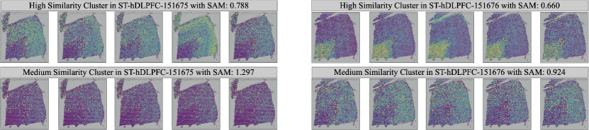
Figure 3. SGEPs from clusters generated by DARLC in dataset (ST-hLDPFC-{5-6}) with high and medium intra-cluster similarity.

4.1. Experimental Settings

Table 2. Gene-gene interaction prediction results for three gene image embeddings. The superior method is bolded.

	ACC (%)
Case	ST-hDLPFC-{1-6}
iBOT	66.58	68.73	68.53	65.88	68.03	67.48
DARLC-C1	76.18	77.20	74.71	73.64	77.85	71.50
DARLC-full	78.11	78.97	77.66	78.74	78.65	73.59

4.1.1. Datasets.

To comprehensively analyze DARLC, we utilize 9 real ST datasets from 6 human dorsolateral prefrontal cortex slices (ST-hDLPFC-{1-6}), 1 human middle temporal gyrus slice (ST-hMTG), 1 human breast cancer slice (ST-hBC), and 1 mouse embryo slice (ST-mEmb). These ST datasets display the spatial expression levels of the entire genome across the corresponding tissue, approximately 18,000 75x75 SGEP images per dataset. Additionally, we use 1 real mass spectrometry imaging dataset from a mouse brain (MSI-hBrain). This dataset displays the spatial expression levels of the entire metabolome, containing 847 110x59 SNIs. We also utilize two artificially sparsified STL-10* and CIFAR-10* datasets with 90% pixels masked, which comprise 13,000 96x96x3 and 60,000 32x32x3 images, respectively. All datasets are available and detailed description can be found in Supplementary 1.4.

4.1.2. Data quality control and preprocessing.

We conform to the conventional procedure for preprocessing ST data, as implemented in the SCANPY package (Wolf et al., 2018). Specifically, we first remove mitochondrial and External RNA Controls Consortium spike-in genes. Then, genes detected in fewer than 10 spots are excluded. To preserve the spatial data integrity, we do not perform quality control on spatial spots. Finally, the gene expression counts are normalized by library size, followed by log-transformation. As for MSI dataset, we utilize traditional precedure total ion current normalization (Fonville et al., 2012).

4.1.3. Cluster Number Inference.

Given the number of image clusters is not known a priori, DARLC can estimate this number using a seeding similarity matrix $\mathcal{S}\in\mathbb{R}^{N\times N}$, where $N$ represents the number of images (Yu et al., 2023). $\mathcal{S}$ is transformed to a graph Laplacian matrix (refer to Supplementary 1.2), $L^{\prime}\in\mathbb{R}^{N\times N}$ as follows:

(23) $$L^{\prime}=L+L^{2},$$

where $L=\mathbb{D}-\mathcal{S}$, $\mathbb{D}$ is $\mathcal{S}$’s degree matrix, and $L^{2}$ aims to enhance the similarity structure. Then the normalized Laplacian matrix can be obtained as:

(24) $$\mathbb{L}=\mathbb{D}^{-\frac{1}{2}}L^{\prime}\mathbb{D}^{-\frac{1}{2}}.$$

The eigenvalues of $\mathbb{L}$ are then ranked as $\lambda_{(1)}\leq\lambda_{(2)}\leq\cdots\leq\lambda_{(N)}$. The number of clusters, denoted as $K$, is inferred as:

(25) $$K={\rm argmax}_{i}\left\{\lambda_{\left(i\right)}-\lambda_{\left(i-1\right)}\right\},\ \ \ \ i=2,\ 3,\ \cdots,\ N.$$

4.1.4. Baselines.

The image clustering benchmark methods include two classic deep clustering method, DEC (Xie et al., 2016) and DAGMM (Zong et al., 2018), as well as five SOTA methods that either improve DEC (e.g.,EDESC (Cai et al., 2022) and IDCEC (Lu et al., 2022)) or incorporate CL (e.g., CC (Li et al., 2021a), DCP (Lin et al., 2022), and CVCL (Chen et al., 2023)). In addition, we include a benchmark method consisting of iBOT (Zhou et al., 2021), which integrates CL and MIM for representation learning, and a boosted GMM for clustering, denoted as iBOT-C.

4.1.5. Implementation Details.

The GAT for data augmentation adopts an encoder including a single attention head with C-512-30 network structure, and a symmetric decoder. In Module I, the shared encoder structure is a ViT comprising four transformer blocks, each having four attention heads, for processing $75\times 75$ input images segmented into $4\times 4$ patches in our case. The MIM decoder follows a D-128-256-512-1024-75*75 residual network. The Module I is pretrained for 50 epochs with a learning rate of 0.001. The nonlinear projection head that bridges Module I and II is a two-layer MLP for normalizing image representations to a dimension size of 32. The iterative joint optimization of representation learning and clustering continues for 50 epochs using Adam optimizer. Given the absence of ground truth in gene cluster labels, we heuristically determine the number of gene clusters for our experiments to achieve an average cluster size of 30 genes, approximating the typical size of a gene pathway  (Zhou et al., 2012).

4.1.6. Evaluation Metrics.

Without ground truth cluster labels, we evaluate the clustering results using the Davies-Bouldin index (DBI) metric  (Davies and Bouldin, 1979):

(26) $$\begin{split}\mathrm{DBI}=\mathrm{~{}}\frac{1}{K}\sum_{i=1}^{K}\max_{i\neq j}\frac{d_{i}+d_{j}}{d_{(i,j)}},d_{i}=\frac{1}{|C_{i}|}\sum_{j=1}^{|C_{i}|}\delta_{c_{i},j},\end{split}$$

where $K$ is the number of clusters, $C_{i}$ the samples in cluster $i$, $\delta_{i,j}$ the distance between instances $i$ and $j$, $c_{i}$ the centroid of cluster $i$. Cluster width $d_{i}$ is the mean intra-cluster distance to $c_{i}$, and $d_{(i,j)}=\delta_{c_{i},c_{j}}$ measures the distance between clusters $i$ and $j$. DBI quantifies the clustering efficiency by measuring the ratio of intra-cluster compactness to inter-cluster separation, with lower scores indicating better clustering. To evaluate clustering from different perspectives, we use two DBI metrics, DBIP and DBIE, based on Pearson and Euclidean distances, respectively (Song et al., 2022).

Table 3. Spatial cofunctional gene clustering results using three image embeddings, with the best method in bolded

. NMI (%)$\uparrow$ Case ST-hDLPFC-{1-6} iBOT 20.56 15.98 15.41 27.05 23.17 25.62 DARLC-C1 66.81 67.81 70.91 65.13 74.62 75.85 DARLC-full 78.11 71.28 79.23 74.34 75.20 75.91

4.2. Clustering Sparse, Noisy Images of Spatial Gene Expressions

Table 1 showcase the performance of DARLC, compared to eight benchmark methods, in clustering SNIs across 12 datasets, evaluated by DBIE and DBIP for unlabeled, NMI and ARI for labeled datasets, the experiment is repeated ten times to obtain the mean and standard deviation of each method’s scores. DARLC consistently scores lowest in DBIE and DBIP for all unlabeled datasets and highest in NMI and ARI for labeled datasets, highlighting its superiority in generating clusters consisting of spatially similar and coherent images. This superiority can be attributed to DARLC’s features in integrating MIM and CL, generating more plausible augmented data, and the robust and adaptable clustering algorithm, as substantiated in our ablation study. In contrast, benchmark methods adopt varied strategies: IDCEC and EDESC leverage a convolutional autoencoder for extracting visual features; iBOT+boosted GMM adopts conventional data augmentation; CC, CVCL and DCP rely solely on CL for representation learning; DAGMM employs an outlier-sensitive GMM for clustering. However, these methods generally demonstrate unstable and suboptimal performance. Overall, compared to the best-performing benchmark method, DARLC achieves an average reduction of approximately 15.98% in DBIE and 18.44% in DBIP across all ST and MSI datasets. Finally, DARLC clusters are divided into high and medium-quality groups using spectral angle mapper (SAM) metric scores (Kruse et al., 1993), with lower SAM indicating greater intra-cluster similarity. To provide a visual illustration of DARLC’s clustering performance, we randomly select one cluster from both the high- and medium-quality groups within each of the ST-hDLPFC-{5-6} datasets. From each of the selected clusters, we then randomly select five genes to be displayed in Figure 3. Figure 3 clearly demonstrates that DARLC effectively groups images with similar expression patterns into the same cluster.

4.3. Evaluating DARLC-generated Gene Image Representations

In this section, we present a comprehensive evaluation of gene image representations produced by the fully implemented DARLC model (denoted as DARLC-full). First, we assess whether representations generated by DARLC-full capture corresponding biosemantics, particularly through pathway enrichment analysis, compared to original gene expressions. Furthermore, we extend our investigation to specific critical downstream tasks: predicting interactions between genes and clustering genes based on spatial cofunctionality. These evaluations are conducted across six distinct datasets (ST-hDLPFC-{1-6}). Additionally, gene image embeddings generated by iBOT and a variant of DARLC (denoted as DARLC-C1), which is deprived of Module II, serve as baselines.

4.3.1. Gene-gene Interaction Prediction.

We employ an MLP-based classifier for predicting gene pair interactions. This is achieved by linear probing using gene image representations generated by DARLC and baseline methods (see Supplementary 1.5). We follow the methodology in (Du et al., 2019), which is based on the Gene Ontology, to acquire the gene-gene interaction ground truth. Theoretically, gene image representations with richer semantic meanings should yield more accurate predictions. As shown by the accuracy scores in Table 2, the classifier yields the most accurate predictions (77.62%±1.85%) using embeddings generated by DARLC-full, and the second most accurate predictions (75.18%±2.17%) using embeddings generated by DARLC-C1, followed by the predictions using iBOT-generated embeddings (67.54%±1.03%).

4.3.2. Spatially Cofunctional Gene Clustering.

Spatially cofunctional genes are those belonging to the same gene family and exhibit similar spatial expression patterns  (Demuth et al., 2006). Their family identities can serve as labels to evaluate the quality of gene image embeddings via clustering. Specifically, our evaluation involves five spatially cofunctional genes from each of the HLA, GABR, RPL, and MT gene families (see Supplementary Figure 1). The Leiden algorithm (Traag et al., 2019) is used to cluster gene image embeddings generated by DARLC-full and the baseline methods. The clustering results, evaluated using the normalized mutual information (NMI) and adjusted rand index (ARI) scores, as shown in Table 3 and Supplementary Table 3, demonstrate that Leiden yields the most accurate clustering with DARLC-full and the second most accurate with DARLC-C1.

In summary, these results collectively highlight the effectiveness of the joint clustering (i.e., DARLC-full surpasses DARLC-C1) and GAT-based data augmentation (i.e., DARLC-C1 surpasses iBOT) in enhancing the quality of gene image representations.

4.4. Ablation Study

Here, we conduct a series of ablation studies on six ST datasets (ST-hDLPFC-{1-6}) to investigate the contributions of DARLC’s components in image clustering. The results, detailed in DBIE and DBIP scores, are presented in Table 4 and Supplementary Table 4. Notably, DARLC’s performance declines most with the CL branch removal (“w/o CLR”), followed by the elimination of Module II (“w/o SMM”) and the substitution of the robust SMM with an outlier-sensitive GMM (“SMM $\rightarrow$ GMM”). We also observed that employing traditional image smoothing methods such as Gaussian Kernel Smoothing (GKS) instead of GAT (“GAT $\rightarrow$ GKS”) on SNIs leads to a decline in DARLC’s performance. Additionally, removing either $\mathcal{L}_{\ell ap}$ (“w/o $\mathcal{L}_{\ell ap}$”) or $\mathcal{L}_{size}$ (“w/o $\mathcal{L}_{size}$”) from the optimization decreases DARLC’s performance, indicated by higher DBIE and DBIP scores. Lastly, “w/o Pretraining” showcases DARLC’s performance at the same clustering training epoch as the complete model but without the initial “warm up” pretraining of Module I. The relative underperformance in the “w/o Pretraining” scenario suggests a slower training convergence compared to the complete model.

Table 4. Ablation study results across six datasets for components in Module I &II and regularization terms. The best result is bolded.

	DBIE$\downarrow$
Case	ST-hDLPFC-{1-6}
w/o CLR	14.35	16.99	8.70	9.23	10.36	15.12
GAT $\rightarrow$ GKS	9.35	10.37	8.98	9.08	8.90	8.95
w/o SMM	11.84	12.19	11.33	11.81	11.49	12.35
SMM $\rightarrow$ GMM	11.49	11.36	11.16	11.31	11.05	11.37
w/o $\mathcal{L}_{\ell ap}$	8.32	10.76	9.02	8.10	9.22	8.12
w/o $\mathcal{L}_{size}$	10.38	8.60	8.11	9.34	8.00	8.28
w/o Pretraining	8.22	8.74	8.38	8.18	7.87	9.09
DARLC-full	7.65	8.06	7.90	7.78	7.41	8.09

5. Conclusion

In this study, we introduce DARLC, a novel algorithm for dual advancement of representation learning and clustering for SNIs. DARLC features in its enhanced data augmentation technique, comprehensive and potent representation learning approach that integrates MIM, CL and clustering, as well as robust and adaptable clustering algorithm. These features collectively contribute to DARLC’s superiority in both image representation learning and clustering, as evidenced by our extensive benchmarks over multiple real datasets and comprehensive ablation studies.

References

- (1)
- Askari (2021) Salar Askari. 2021. Fuzzy C-Means clustering algorithm for data with unequal cluster sizes and contaminated with noise and outliers: Review and development. Expert Systems with Applications 165 (2021), 113856.
- Bao et al. (2021) Hangbo Bao, Li Dong, Songhao Piao, and Furu Wei. 2021. Beit: Bert pre-training of image transformers. arXiv preprint arXiv:2106.08254 (2021).
- Cai et al. (2022) Jinyu Cai, Jicong Fan, Wenzhong Guo, Shiping Wang, Yunhe Zhang, and Zhao Zhang. 2022. Efficient deep embedded subspace clustering. In Proceedings of the IEEE/CVF Conference on Computer Vision and Pattern Recognition. 1–10.
- Cai et al. (2020) Tiffany Tianhui Cai, Jonathan Frankle, David J Schwab, and Ari S Morcos. 2020. Are all negatives created equal in contrastive instance discrimination? arXiv preprint arXiv:2010.06682 (2020).
- Caron et al. (2020) Mathilde Caron, Ishan Misra, Julien Mairal, Priya Goyal, Piotr Bojanowski, and Armand Joulin. 2020. Unsupervised learning of visual features by contrasting cluster assignments. Advances in neural information processing systems 33 (2020), 9912–9924.
- Caron et al. (2021) Mathilde Caron, Hugo Touvron, Ishan Misra, Hervé Jégou, Julien Mairal, Piotr Bojanowski, and Armand Joulin. 2021. Emerging properties in self-supervised vision transformers. In Proceedings of the IEEE/CVF international conference on computer vision. 9650–9660.
- Chen et al. (2023) Jie Chen, Hua Mao, Wai Lok Woo, and Xi Peng. 2023. Deep Multiview Clustering by Contrasting Cluster Assignments. arXiv preprint arXiv:2304.10769 (2023).
- Chen et al. (2020) Ting Chen, Simon Kornblith, Mohammad Norouzi, and Geoffrey Hinton. 2020. A simple framework for contrastive learning of visual representations. In International conference on machine learning. PMLR, 1597–1607.
- Chen and He (2021) Xinlei Chen and Kaiming He. 2021. Exploring simple siamese representation learning. In Proceedings of the IEEE/CVF conference on computer vision and pattern recognition. 15750–15758.
- Davies and Bouldin (1979) David L Davies and Donald W Bouldin. 1979. A cluster separation measure. IEEE transactions on pattern analysis and machine intelligence 2 (1979), 224–227.
- Demuth et al. (2006) Jeffery P Demuth, Tijl De Bie, Jason E Stajich, Nello Cristianini, and Matthew W Hahn. 2006. The evolution of mammalian gene families. PloS one 1, 1 (2006), e85.
- Denize et al. (2023) Julien Denize, Jaonary Rabarisoa, Astrid Orcesi, Romain Hérault, and Stéphane Canu. 2023. Similarity contrastive estimation for self-supervised soft contrastive learning. In Proceedings of the IEEE/CVF Winter Conference on Applications of Computer Vision. 2706–2716.
- Dong and Zhang (2022) Kangning Dong and Shihua Zhang. 2022. Deciphering spatial domains from spatially resolved transcriptomics with an adaptive graph attention auto-encoder. Nature communications 13, 1 (2022), 1739.
- Dosovitskiy et al. (2020) Alexey Dosovitskiy, Lucas Beyer, Alexander Kolesnikov, Dirk Weissenborn, Xiaohua Zhai, Thomas Unterthiner, Mostafa Dehghani, Matthias Minderer, Georg Heigold, Sylvain Gelly, et al. 2020. An image is worth 16x16 words: Transformers for image recognition at scale. arXiv preprint arXiv:2010.11929 (2020).
- Du et al. (2019) Jingcheng Du, Peilin Jia, Yulin Dai, Cui Tao, Zhongming Zhao, and Degui Zhi. 2019. Gene2vec: distributed representation of genes based on co-expression. BMC genomics 20 (2019), 7–15.
- Fonville et al. (2012) Judith M Fonville, Claire Carter, Olivier Cloarec, Jeremy K Nicholson, John C Lindon, Josephine Bunch, and Elaine Holmes. 2012. Robust data processing and normalization strategy for MALDI mass spectrometric imaging. Analytical chemistry 84, 3 (2012), 1310–1319.
- Gao et al. (2022) Peng Gao, Teli Ma, Hongsheng Li, Ziyi Lin, Jifeng Dai, and Yu Qiao. 2022. Convmae: Masked convolution meets masked autoencoders. arXiv preprint arXiv:2205.03892 (2022).
- Grill et al. (2020) Jean-Bastien Grill, Florian Strub, Florent Altché, Corentin Tallec, Pierre Richemond, Elena Buchatskaya, Carl Doersch, Bernardo Avila Pires, Zhaohan Guo, Mohammad Gheshlaghi Azar, et al. 2020. Bootstrap your own latent-a new approach to self-supervised learning. Advances in neural information processing systems 33 (2020), 21271–21284.
- Guo et al. (2017) Xifeng Guo, Long Gao, Xinwang Liu, and Jianping Yin. 2017. Improved deep embedded clustering with local structure preservation.. In Ijcai, Vol. 17. 1753–1759.
- He et al. (2022) Kaiming He, Xinlei Chen, Saining Xie, Yanghao Li, Piotr Dollár, and Ross Girshick. 2022. Masked autoencoders are scalable vision learners. In Proceedings of the IEEE/CVF conference on computer vision and pattern recognition. 16000–16009.
- He et al. (2020) Kaiming He, Haoqi Fan, Yuxin Wu, Saining Xie, and Ross Girshick. 2020. Momentum contrast for unsupervised visual representation learning. In Proceedings of the IEEE/CVF conference on computer vision and pattern recognition. 9729–9738.
- Huang et al. (2023) Zhicheng Huang, Xiaojie Jin, Chengze Lu, Qibin Hou, Ming-Ming Cheng, Dongmei Fu, Xiaohui Shen, and Jiashi Feng. 2023. Contrastive masked autoencoders are stronger vision learners. IEEE Transactions on Pattern Analysis and Machine Intelligence (2023).
- Kruse et al. (1993) Fred A Kruse, AB Lefkoff, y JW Boardman, KB Heidebrecht, AT Shapiro, PJ Barloon, and AFH Goetz. 1993. The spectral image processing system (SIPS)—intera-ctive visualization and analysis of imaging spectrometer data. Remote sensing of environment 44, 2-3 (1993), 145–163.
- Li et al. (2018) Fengfu Li, Hong Qiao, and Bo Zhang. 2018. Discriminatively boosted image clustering with fully convolutional auto-encoders. Pattern Recognition 83 (2018), 161–173.
- Li et al. (2021b) Junnan Li, Pan Zhou, Caiming Xiong, and Steven C. H. Hoi. 2021b. Prototypical Contrastive Learning of Unsupervised Representations. In 9th International Conference on Learning Representations, ICLR 2021, Virtual Event, Austria, May 3-7, 2021. OpenReview.net. https://openreview.net/forum?id=KmykpuSrjcq
- Li et al. (2021a) Yunfan Li, Peng Hu, Zitao Liu, Dezhong Peng, Joey Tianyi Zhou, and Xi Peng. 2021a. Contrastive clustering. In Proceedings of the AAAI conference on artificial intelligence, Vol. 35. 8547–8555.
- Liebel and Körner (2018) Lukas Liebel and Marco Körner. 2018. Auxiliary tasks in multi-task learning. arXiv preprint arXiv:1805.06334 (2018).
- Lin et al. (2022) Yijie Lin, Yuanbiao Gou, Xiaotian Liu, Jinfeng Bai, Jiancheng Lv, and Xi Peng. 2022. Dual contrastive prediction for incomplete multi-view representation learning. IEEE Transactions on Pattern Analysis and Machine Intelligence 45, 4 (2022), 4447–4461.
- Lu et al. (2022) Hu Lu, Chao Chen, Hui Wei, Zhongchen Ma, Ke Jiang, and Yingquan Wang. 2022. Improved deep convolutional embedded clustering with re-selectable sample training. Pattern Recognition 127 (2022), 108611.
- Lu et al. (2021) Yadong Lu, Julian Collado, Daniel Whiteson, and Pierre Baldi. 2021. Sparse autoregressive models for scalable generation of sparse images in particle physics. Physical Review D 103, 3 (2021), 036012.
- Ren et al. (2022) Yazhou Ren, Jingyu Pu, Zhimeng Yang, Jie Xu, Guofeng Li, Xiaorong Pu, Philip S Yu, and Lifang He. 2022. Deep clustering: A comprehensive survey. arXiv preprint arXiv:2210.04142 (2022).
- Sloka (2023) Scott Sloka. 2023. Image denoising in astrophotography-an approach using recent network denoising models. Journal of the British Astronomical Association 133, 4 (2023).
- Song et al. (2022) Tianci Song, Kathleen K Markham, Zhuliu Li, Kristen E Muller, Kathleen Greenham, and Rui Kuang. 2022. Detecting spatially co-expressed gene clusters with functional coherence by graph-regularized convolutional neural network. Bioinformatics 38, 5 (2022), 1344–1352.
- Ståhl et al. (2016) Patrik L Ståhl, Fredrik Salmén, Sanja Vickovic, Anna Lundmark, José Fernández Navarro, Jens Magnusson, Stefania Giacomello, Michaela Asp, Jakub O Westholm, Mikael Huss, et al. 2016. Visualization and analysis of gene expression in tissue sections by spatial transcriptomics. Science 353, 6294 (2016), 78–82.
- Traag et al. (2019) Vincent A Traag, Ludo Waltman, and Nees Jan Van Eck. 2019. From Louvain to Leiden: guaranteeing well-connected communities. Scientific reports 9, 1 (2019), 5233.
- Velickovic et al. (2018) Petar Velickovic, Guillem Cucurull, Arantxa Casanova, Adriana Romero, Pietro Liò, and Yoshua Bengio. 2018. Graph Attention Networks. In 6th International Conference on Learning Representations, ICLR 2018, Vancouver, BC, Canada, April 30 - May 3, 2018, Conference Track Proceedings. OpenReview.net. https://openreview.net/forum?id=rJXMpikCZ
- Wang and Jiang (2021) Jinghua Wang and Jianmin Jiang. 2021. Unsupervised deep clustering via adaptive GMM modeling and optimization. Neurocomputing 433 (2021), 199–211.
- Wang et al. (2023) Yuxing Wang, Wenguan Wang, Dongfang Liu, Wenpin Hou, Tianfei Zhou, and Zhicheng Ji. 2023. GeneSegNet: a deep learning framework for cell segmentation by integrating gene expression and imaging. Genome Biology 24, 1 (2023), 235.
- Wolf et al. (2018) F Alexander Wolf, Philipp Angerer, and Fabian J Theis. 2018. SCANPY: large-scale single-cell gene expression data analysis. Genome biology 19 (2018), 1–5.
- Xie et al. (2016) Junyuan Xie, Ross Girshick, and Ali Farhadi. 2016. Unsupervised deep embedding for clustering analysis. In International conference on machine learning. PMLR, 478–487.
- Xie et al. (2022) Zhenda Xie, Zheng Zhang, Yue Cao, Yutong Lin, Jianmin Bao, Zhuliang Yao, Qi Dai, and Han Hu. 2022. Simmim: A simple framework for masked image modeling. In Proceedings of the IEEE/CVF Conference on Computer Vision and Pattern Recognition. 9653–9663.
- Yin et al. (2023) Jun Yin, Haowei Wu, and Shiliang Sun. 2023. Effective sample pairs based contrastive learning for clustering. Information Fusion 99 (2023), 101899.
- Yu et al. (2023) Xiaokang Yu, Xinyi Xu, Jingxiao Zhang, and Xiangjie Li. 2023. Batch alignment of single-cell transcriptomics data using deep metric learning. Nature Communications 14, 1 (2023), 960.
- Zheng et al. (2021) Mingkai Zheng, Fei Wang, Shan You, Chen Qian, Changshui Zhang, Xiaogang Wang, and Chang Xu. 2021. Weakly supervised contrastive learning. In Proceedings of the IEEE/CVF International Conference on Computer Vision. 10042–10051.
- Zhou et al. (2012) Hufeng Zhou, Jingjing Jin, Haojun Zhang, Bo Yi, Michal Wozniak, and Limsoon Wong. 2012. IntPath–an integrated pathway gene relationship database for model organisms and important pathogens. In BMC systems biology, Vol. 6. BioMed Central, 1–17.
- Zhou et al. (2021) Jinghao Zhou, Chen Wei, Huiyu Wang, Wei Shen, Cihang Xie, Alan Yuille, and Tao Kong. 2021. ibot: Image bert pre-training with online tokenizer. arXiv preprint arXiv:2111.07832 (2021).
- Zhu et al. (2021) Jiaqiang Zhu, Shiquan Sun, and Xiang Zhou. 2021. SPARK-X: non-parametric modeling enables scalable and robust detection of spatial expression patterns for large spatial transcriptomic studies. Genome biology 22, 1 (2021), 1–25.
- Zong et al. (2018) Bo Zong, Qi Song, Martin Renqiang Min, Wei Cheng, Cristian Lumezanu, Daeki Cho, and Haifeng Chen. 2018. Deep autoencoding gaussian mixture model for unsupervised anomaly detection. In International conference on learning representations.