Abstract: This paper constructs unique compactly supported functions in Sobolev spaces that have minimal norm, maximal support, and maximal central value, under certain renormalizations. They may serve as optimized basis functions in interpolation or approximation, or as shape functions in meshless methods for PDE solving. Their norm is useful for proving upper bounds for convergence rates of interpolation in Sobolev spaces $H_{2}^{m}(\mathbb{R}^{d})$, and this paper gives the correct rate $m-d/2$ that arises as convergence like $h^{m-d/2}$ for interpolation at meshwidth $h\to 0$ or a blow-up like $r^{-(m-d/2)}$ for norms of compactly supported functions with support radius $r\to 0$. In Hilbert spaces with infinitely smooth reproducing kernels, like Gaussians or inverse multiquadrics, there are no compactly supported functions at all, but in spaces with limited smoothness, compactly supported functions exist and can be optimized in the above way. The construction is described in Hilbert space via projections, and analytically via trace operators. Numerical examples are provided.

MSC Classification:
65D12, 41A15, 46E35, 65D07, 47B32, 35A08, 35B07
Keywords:
Radial Basis Functions, Splines, bump functions, shape functions, Sobolev Spaces

1 Introduction

In general, a test function is a smooth compactly supported (CS) function, sometimes assumed to be of infinite smoothness, and often called a bump function. Such functions are very useful in Analysis at various places, e.g. as mollifiers or as trial functions.

In reproducing kernel Hilbert spaces like global Sobolev spaces, they also help to prove certain results, e.g. the optimal rates of approximations of derivatives by scalable stencils [6].

But a closer look at test functions in kernel-based spaces reveals that they may not even exist in general. Consequently, this paper focuses on test functions in kernel-based spaces, their existence, their properties, and their applications. While writing, it emerged that there seems to be no general theory of compactly supported functions in Sobolev spaces, and this paper tries to fill the gap in that generality.

First, the basics of kernel-based spaces are stated, for fixing notation and the context. Section 3 turns to compactly supported functions, and Section 4 provides a simple application to the error analysis of interpolation.

Then Section 5 shows that compactly supported functions may simply not exist at all, if Fourier transforms of kernels decay exponentially. But in cases of algebraic decay, like for the Matérn kernel generating Sobolev spaces, there exists unique norm-minimal functions $b_{r}^{*}$ with support on the ball $B_{r}(0)$ of radius $r$ around the origin and value $b_{r}^{*}(0)=1$. By uniqueness, they are necessarily radial.

Other properties of these functions and their norms are proven in Section 6. When norms are kept bounded, they have the maximal possible value at zero and the least possible support radius. Section 7 considers the behaviour of the optimal norm $\|b_{r}^{*}\|$ as a function of $r$, proving $\|b_{r}^{*}\|=\Theta(r^{-m+d/2})$ for $r\to 0$ in case of Sobolev space $H_{2}^{m}(\mathbb{R}^{d})$. This works by scaling arguments, and it turns out that downscaling of optimal functions to a smaller support radius loses optimality, but still has asymptotically the same rate as above.

Then Section 8 gives a characterization in terms of Hilbert space arguments via projections, and Section 9 applies standard Sobolev space trace arguments to get a computable representation. Numerical examples are added in Section 10, while Section 11 summarizes the results and raises quite a number of issues that require further investigation.

2 Basics of Spaces and Kernels

Let $K$ be a continuous symmetric positive definite translation-invariant real-valued kernel on $\mathbb{R}^{d}\times\mathbb{R}^{d}$. It generates a native Hilbert space $\mathcal{K}$ of functions on $\mathbb{R}^{d}$ with inner product $(.,.)_{K}$ and the remarkable properties

$$\begin{array}[]{rcll}K(x,y)&=&(K(x,\cdot),K(y,\cdot))_{K}&\hbox{ for all }x,\,y\in\mathbb{R}^{d},\\ f(x)&=&(f,K(x,\cdot))_{K}&\hbox{ for all }x\in\mathbb{R}^{d},\,f\in\mathcal{K},\\ K(x,y)&=&(\delta_{x},\delta_{y})_{\mathcal{K}^{*}}&\hbox{ for all }x,\,y\in\mathbb{R}^{d}.\\ \end{array}$$

All delta functionals $\delta_{x}\;:\;f\mapsto f(x)$ are continuous and have a kernel translate $K(x,\cdot)$ as their Riesz representer. The space $\mathcal{K}$ is the closure of all kernel translates under the above inner product. The theory of kernel-based spaces is treated extensively in the books [3, 22, 9] and an earlier lecture note [14], but we recall the basic facts for convenience of readers and for fixing notation, as far as needed in this paper.

In Spatial Statistics, kernels arise as covariance functions of a mean-zero random field $R$ on $\mathbb{R}^{d}$ in the sense that each $x\in\mathbb{R}^{d}$ carries a zero-mean second-order random variable $R(x)$ such that $K(x,y)=Cov(R(x),R(y))\hbox{ for all }x,y\in\mathbb{R}^{d}$.

In Real Analysis, Sobolev spaces $H_{2}^{m}(\mathbb{R}^{d})$ for $m>d/2$ are Hilbert spaces generated by Whittle-Matérn kernels

$$K(x,y)=\|x-y\|_{2}^{m-d/2}K_{m-d/2}(\|x-y\|_{2})$$

up to factors, where $K_{\nu}$ is the modified Bessel function of second kind. This case is very important as well in Spatial Statistics, see [12] for an overview. We use the $H_{2}^{m}(\mathbb{R}^{d})$ notation instead of $W_{2}^{m}(\Omega)$, because we work on the full space and define Sobolev spaces via Fourier transforms.

The recovery of functions $f$ from values $f(x_{1}),\ldots,f(x_{n})$ on a set $X_{n}=\{x_{1},\ldots,x_{n}\}\subset\mathbb{R}^{d}$ of data points can be uniquely done by a function $s_{X_{n},f}\in\mathcal{K}$ generated by the kernel translates $K(x_{1},\cdot),\ldots,K(x_{n},\cdot)$, and the pointwise error bound is

$$|f(x)-s_{X_{n},f}(x)|\leq P_{X_{n}}(x)\|f\|_{K}\hbox{ for all }x\in\mathbb{R}^{d},\,f\in\mathcal{K}.$$ (1)

Here, the Power Function $P_{X}\;:\;\mathbb{R}^{d}\to\mathbb{R}$ arises. It is the distance of $\delta_{x}$ to the span of all $\delta_{x_{j}},\;1\leq j\leq n$ in the norm of the dual $\mathcal{K}^{*}$. In Spatial Statistics, $s_{X,f}(x)$ is the best unbiased linear predictor for $f(x)$ given all $f(x_{1}),\ldots,f(x_{n})$ under the random field with covariance function $K$, and $P_{X_{n}}^{2}(x)$ is the variance of this prediction. For what follows, the Power Function has the alternative definition

$$P_{X_{n}}(x)=\sup\{f(x)\;:\;f\in\mathcal{K},\;\|f\|_{K}\leq 1,\;f(x_{j})=0,\;1\leq j\leq n\}.$$ (2)

3 Bump Functions

We look at a special case of compactly supported functions first. General compactly supported functions will come up later.

Definition 1.

A bump function of support radius $r$ is an element of the set

$${{\mathcal{B}}_{r}:=\{b\in\mathcal{K}\;:\;b(0)=1,b(y)=0\;\hbox{ for all }\;\|y\|_{2}\geq r\}}$$

of functions on $\mathcal{K}$.

In spaces $\mathcal{K}$ consisting of analytic functions, the set ${\mathcal{B}}$ will be empty, and Corollary 1 in Section 5 gives a sufficient criterion in terms of kernel smoothness. But for most of the paper, existence of bump functions is assumed, and then they exist for all scales, as shown in Section 5.

This calls for optimizing bump functions, and a typical application will be in Section 4.

Definition 2.

A bump function $b_{r}^{*}\in{\mathcal{B}}_{r}$ is norm-minimal, if

$$\|b_{r}^{*}\|_{K}=\displaystyle{\inf\{\|b\|_{K}\;:\;b\in{\mathcal{B}}_{r}\}}=:\beta(r),$$

and we call $\beta\;:\;\mathbb{R}_{>0}\to\mathbb{R}_{>0}$ the bump norm function.

These functions are the main topic of the paper, but many results extend to general compactly supported functions.

4 A Simple Application

The following result is a good motivation to investigate bump functions. Its consequences are elaborated in [17] concerning Trade-off Principles between errors and stability. Let $X_{n}=\{x_{1},\ldots,x_{n}\}$ be a set of data points in $\mathbb{R}^{d}$, and define the distance

$$dist(x,X_{n})=\displaystyle{\min_{1\leq j\leq n}\|x-x_{j}\|_{2}}$$

from a point $x$ to $X_{n}$.

Theorem 1.

Then the Power Function $P_{X}$ satisfies

$$P_{X}(x)\geq\displaystyle{\frac{1}{\|b\|_{K}}}$$ (3)

for all bump functions $b$ with support radius $dist(x,X_{n})$ or larger.

Proof.

Any such bump function has zero as its interpolant, and thus

$$1=|b(x)|\leq P_{X}(x)\|b\|_{K}$$

by the standard error bound (1). ∎

Inequalities like this provide lower bounds for pointwise interpolation errors, and these bounds are best if the norm is minimized. This is why we look at compactly supported functions with minimal norm.

We shall see in (5) that in Sobolev spaces $H_{2}^{m}(\mathbb{R}^{d})$ the bump norm function $\beta(r)$ behaves like $r^{d/2-m}$, and thus (3) yields a simple counterpart to the standard upper bounds of the Power Function, proving their asymptotic optimality. An earlier but much more complicated proof goes back to [13]. If the error is measured in $\mathcal{K}$, all other interpolation techniques have larger errors. This proves that (3) is also a lower bound for errors of all other interpolation processes in Sobolev spaces. The paper [6] works in a somewhat different context, but it also uses bump functions to prove the optimal possible convergence rate for interpolation and derivative approximation in Sobolev spaces.

Papers using bump functions for different purposes are [11, 7, 5, 10], but there will be many others. None of these papers look at bump functions in detail.

This calls for an investigation of bump functions and the bump norm function for more general cases, but it turns out that this runs into serious unexpected difficulties that are interesting in their own right.

5 Existence Problems

It is clear that compactly supported functions exist in all kernel–based spaces that only require certain finite smoothness properties, like Sobolev spaces $H_{2}^{m}(\mathbb{R}^{d})$ for $m>d/2$. Wendland functions are examples that even use the kernel itself [21, 15].

For other kernel-bases spaces, e.g. those based on multiquadrics and Gaussians, the existence of compactly supported functions is a serious problem. Clearly, there are $C^{\infty}$ functions with compact support, but one has to find some that lie in the given native Hilbert space, i.e. the Fourier transform has to satisfy a specific decay property. The following negative result uses the fact that exponential decay of Fourier transforms implies local analyticity around zero, contradicting compact support when applied to compactly supported functions.

Lemma 1.

Assume that the $d$-variate Fourier transform $\hat{f}$ of some Fourier-transformable function $f$ on $\mathbb{R}^{d}$ has exponential decay

$$|\hat{f}(\omega)|\leq C\exp(-c\|\omega\|_{2})\hbox{ for all }\omega\in\mathbb{R}^{d}.$$

Then the function is analytic in a ball around zero of radius proportional to $c$, with a factor depending on $C$ and $d$.

Proof.

The derivatives of $f$ at zero are bounded by

$$\begin{array}[]{rcl}|D^{\alpha}f(0)|&\leq&(2\pi)^{-d/2}\displaystyle{\int_{\mathbb{R}^{d}}|\hat{f}(\omega)||(i\omega)^{\alpha}|d\omega}\\ &\leq&(2\pi)^{-d/2}C\displaystyle{\int_{\mathbb{R}^{d}}\exp(-c\|\omega\|_{2})|\omega^{\alpha}|d\omega}\\ &\leq&(2\pi)^{-d/2}C\displaystyle{\int_{\mathbb{R}^{d}}\exp(-c\|\omega\|_{1}/\sqrt{d})|\omega|^{|\alpha|}d\omega}\\ &\leq&(2\pi)^{-d/2}C\displaystyle{\prod_{j=1}^{d}\int_{\mathbb{R}}\exp(-c|\omega_{j}|/\sqrt{d})|\omega_{j}|^{\alpha_{j}}d\omega_{j}}\\ &\leq&(2\pi)^{-d/2}C\displaystyle{2^{d}\left(\frac{\sqrt{d}}{c}\right)^{d+|\alpha|}\alpha!}\\ \end{array}$$

due to

$$\begin{array}[]{rcl}\displaystyle{\int_{\mathbb{R}}\exp(-c|t|/\sqrt{d})|t|^{n}dt}&=&2\displaystyle{\int_{0}^{\infty}\exp(-ct/\sqrt{d})t^{n}dt}\\ &=&2\displaystyle{\frac{\sqrt{d}}{c}\int_{0}^{\infty}\exp(-s)\left(\frac{s\sqrt{d}}{c}\right)^{n}ds}\\ &=&2\displaystyle{\left(\frac{\sqrt{d}}{c}\right)^{n+1}\int_{0}^{\infty}\exp(-s)s^{n}ds}\\ &=&2\displaystyle{\left(\frac{\sqrt{d}}{c}\right)^{n+1}n!}.\end{array}$$

This implies convergence of the Taylor series in a region

$$\{x\in\mathbb{R}^{d}\;:\;|x_{i}|\leq r_{i},\;1\leq i\leq d\}$$

around zero defined by a vector $r=(r_{1},\ldots,r_{d})$ of adjoint radii of convergence, if

$$\overline{\lim}_{|\alpha|\to\infty}\left|\frac{D^{\alpha}f(0)}{\alpha!}r^{\alpha}\right|^{\frac{1}{|\alpha|}}\leq 1$$

holds [19]. Up to $d$-dependent or constant factors, we have to look at

$$\left|\frac{D^{\alpha}f(0)}{\alpha!}\right|^{1/|\alpha|}\leq\left(\frac{\sqrt{d}}{c}\right)^{1+d/|\alpha|}$$

to get the assertion. ∎

Gaussians admit arbitrarily large $c$, while inverse multiquadrics have a fixed maximal $c$ depending on the kernel parameters.

Theorem 2.

The native space of the Gaussian consists of globally analytic functions, i.e. the local power series expansions all exist and converge globally. The native space of $d$-variate inverse multiquadrics generated by the kernel $K(x,y)=(1+\|x-y\|_{2}^{2})^{-m}$ consists of locally analytic functions, i.e. the local power series expansions all exist and converge with at least a fixed radius of convergence.∎

Applying analytic continuation if necessary, we get

Corollary 1.

In spaces generated by kernels with at least exponentially decaying Fourier transform, there are no compactly supported functions. ∎

Consequently, all argumentations using compactly supported functions fail for such cases.

These results are not really surprising. Recall that there are no compactly functions in univariate complex analysis or in spaces of harmonic functions, by the Maximum Principle. In addition, kernels arising from the Hausdorff-Bernstein-Widder representation are analytic and therefore never compactly supported. The above result is slightly different, but similarly negative.

Other cases of Native Spaces without compactly supported functions are those whose kernels have power series expansions in the domain of interest. These are handled in [23, 24].

We now prove existence of norm-minimal bump functions, the generalization to compactly supported functions being evident later.

Theorem 3.

If the set ${\mathcal{B}}_{r}$ of bump functions of radius $r$ is not empty, the bump norm function $\beta(r)$ is attained at a unique bump function $b_{r}^{*}\in{\mathcal{B}}_{r}$, i.e. $\beta(r)=\|b^{*}_{r}\|_{K}$.

Proof.

This follows from a standard variational argument. We start with an admissible bump function $\tilde{b}_{r}$ and approximate it from the closed linear subspace

$${{\mathcal{B}}^{0}_{r}:=\{b\in\mathcal{K}\;:\;b(0)=0,\;b(y)=0\;\hbox{ for all }\;\|y\|_{2}\geq r\}}$$

to get some $\tilde{b}_{r}^{0}\in{\mathcal{B}}^{0}_{r}$ with the orthogonality property

$$(\tilde{b}_{r}-\tilde{b}_{r}^{0},b_{r}^{0})_{K}=0\hbox{ for all }b_{r}^{0}\in{\mathcal{B}}^{0}_{r}.$$

Then we define $b_{r}^{*}:=\tilde{b}_{r}-\tilde{b}_{r}^{0}\in{\mathcal{B}}_{r}$ and take an arbitrary $b_{r}\in{\mathcal{B}}_{r}$ to get

$$\begin{array}[]{rcl}\|b_{r}\|_{K}^{2}&=&\|b_{r}-b_{r}^{*}+b_{r}^{*}\|_{K}^{2}\\ &=&\|b_{r}-b_{r}^{*}\|_{K}^{2}+2(b_{r}-b_{r}^{*},b_{r}^{*})_{K}+\|b_{r}^{*}\|_{K}^{2}\\ &=&\|b_{r}-b_{r}^{*}\|_{K}^{2}+\|b_{r}^{*}\|_{K}^{2}\\ &\geq&\|b_{r}^{*}\|_{K}^{2}.\\ \end{array}$$

∎

The proof generalizes to any compact domain $\Omega\subset\mathbb{R}^{d}$ and an arbitrary point $x$ in its interior for fixing the value 1. Uniqueness follows similarly, and implies

Corollary 2.

For Radial Basis Functions (RBFs), norm-minimal centralized bump functions on balls are radial, if they exist. ∎

This makes it easy to deal with such functions, once the radial form is known or calcutated to sufficient precision.

6 Properties of Bump Functions

From the definition, we have

Theorem 4.

Norms $\|b_{r}^{*}\|_{K}=\beta(r)$ of optimal bump functions $b_{r}^{*}$ increase with decreasing radius.

A second optimality principle is

Theorem 5.

Norm-minimal bump functions have maximal support radius under all bump functions with norm up to one.

Proof.

Assume a bump function $b_{\rho}$ for radius $\rho<r$. Then

$$\|b_{\rho}\|_{K}\geq\beta(\rho)\geq\beta(r)=\|b_{r}^{*}\|_{K}.$$

∎

The bump norm function cannot decrease to zero for large $r$, because there is a positive lower bound:

Lemma 2.

$$\beta^{2}(r)\geq 1/K(0,0)\hbox{ for all }r>0.$$

Proof.

Let $b$ be any bump function at $0$, of arbitrary radius $r$. Then

$$1=b(0)=(b,K(0,\cdot))_{K}\leq\|b\|_{K}\|K(0,\cdot)\|_{K}=\|b\|_{K}\sqrt{K(0,0)}.$$

∎

This is just a special case of the general embedding inequality

$$|f(x)|=|(f,K(x-\cdot)|\leq\|f\|_{K}\|K(x-\cdot)\|_{K}=\|f\|_{K}\sqrt{K(0,0)}\hbox{ for all }f\in\mathcal{K},\;x\in\mathbb{R}^{d}.$$

A third optimality is

Theorem 6.

Under all bump functions with norm up to one, the maximum value at zero is attained for $b_{r}^{*}/\|b_{r}^{*}\|_{K}$.

Proof.

The optimal value is surely not less than $1/\|b_{r}^{*}\|_{K}$. If $b_{r}$ is any bump function with $\|b_{r}\|_{K}\leq 1$, the function $b_{r}/b_{r}(0)$ is admissible for norm minimality, and thus

$${\frac{1}{b_{r}(0)}}\geq\displaystyle{\frac{\|b_{r}\|_{K}}{b_{r}(0)}}\geq\|b_{r}^{*}\|_{K}$$

proves that the optimal value is at most $1/\|b_{r}^{*}\|_{K}$. ∎

We can rewrite this as

$${\frac{1}{\|b_{r}^{*}\|_{K}}}=\sup\{f(0)\;:\;\|f\|_{K}\leq 1,\;f(x)=0\hbox{ for all }\|x\|_{2}\geq r\}$$

and compare with (2) to get the Power Function value $P_{\mathbb{R}^{d}\setminus B_{r}(0)}(0)$ for transfinite interpolation on all points outside the ball $B_{r}(0)$. Note that this realizes the optimal case in (3).

7 Scaling Laws

Now we check bump functions under scaling. To avoid clashes of indices, we use a scaling operator $S_{r}$ acting on functions $f$ on $\mathbb{R}^{d}$ as $S_{r}(f)(x)=f(x/r)\hbox{ for all }x\in\mathbb{R}^{d}$ and $r>0$. If $f$ is supported on a ball $B_{1}(0)$ with radius $r$ around the origin, the scaled function $S_{r}(f)$ is supported on the ball $B_{r}(0)$.

But norm-minimality does not scale that way. If the kernel $K$ is fixed, the optimal bump function $b^{*}_{1}$ for radius $1$ may be scaled into $S_{1}b^{*}_{1}$ to be admissible on $B_{r}(0)$, but this need not be equal to $b^{*}_{r}$. By norm-minimality,

$$\|b^{*}_{r}\|_{K}\leq\|S_{r}b^{*}_{1}\|_{K},$$

and this is all we know. Figure 2 below demonstrates numerically that these two differ, because the shape of $b_{r}^{*}$ changes with $r$ in a nontrivial way.

But scaling functions is also related to scaling kernels. Therefore we locally change the notation $b_{r}^{*}$ to $b_{r,K}^{*}$ if the kernel $K$ is used, and we may scale kernels $K$ with $S_{r}$ into $S_{r}K$ as well. However, since $\|f\|_{K}=\|S_{r}f\|_{S_{r}K}$ holds by [10] for all functions in the native space of $K$, we can apply this to all non-optimal bump functions of the appropriate support radii to get

$$\|S_{r}b^{*}_{1,K}\|_{S_{r}K}=\|b^{*}_{1,K}\|_{K}=\inf\|b_{1}\|_{K}=\inf\|S_{r}b_{1}\|_{S_{r}K}=\inf\|b_{r}\|_{S_{r}K}=\|b^{*}_{r,S_{r}K}\|_{S_{r}K}.$$

Therefore the law

$$S_{r}b^{*}_{1,K}=b^{*}_{r,S_{r}K}$$

connects scaling of norm-minimal bump functions with scaling of the kernel.

But it is more interesting to fix the kernel and vary the radius $r$. We focus on kernels $K$ with

$$\hat{K}(\omega)=\Theta(1+\|\omega\|_{2}^{-\beta}),\;\omega\in\mathbb{R}^{d}$$ (4)

with $\beta>d$ and a positive constant $C$. For the Matérn kernel generating Sobolev space $H_{2}^{m}(\mathbb{R}^{d})$ we have $\beta=2m>d$.

We bound the $d$–variate Fourier transform of any scaled function $S_{r}f(x)=f(x/r)$ via $\widehat{S_{r}f}(\omega)=r^{d}\hat{f}(r\omega)$ to get

$$\begin{array}[]{rcl}\|S_{r}f\|_{K}^{2}&=&\displaystyle{\int_{\mathbb{R}^{d}}|\widehat{S_{r}f}(\omega)|^{2}(1+\|\omega\|_{2}^{\beta})d\omega}\\ &=&\displaystyle{r^{2d}\int_{\mathbb{R}^{d}}|\hat{f}(r\omega)|^{2}(1+r^{-\beta}\|r\omega\|_{2}^{\beta})d\omega}\\ &=&\displaystyle{r^{d-\beta}\int_{\mathbb{R}^{d}}|\hat{f}(\eta)|^{2}(r^{\beta}+\|\eta\|_{2}^{\beta})d\eta}.\end{array}$$

up to constant factors. Now for $r\leq 1$ we find

$$\begin{array}[]{rcl}\|S_{r}f\|_{K}^{2}&\leq&r^{d-\beta}\|f\|_{K}^{2},\end{array}$$

and for lower bounds we use

$$\begin{array}[]{rcl}\|S_{r}f\|_{K}^{2}&\geq&r^{d-\beta}|f|_{K}^{2}\\ \end{array}$$

using the correspondent seminorm. When we apply all of this to bump functions, the seminorm can be bounded below by the norm up to a factor, due to Poincaré inequalities.

Theorem 7.

In spaces generated by kernels with (4), the bump norm function behaves like

$$\beta(r)=\|b_{r}^{*}\|_{K}=\Theta(r^{d/2-\beta/2})\hbox{ for }r\to 0.$$ (5)

In Sobolev space $H_{2}^{m}(\mathbb{R}^{d})$, this holds for $\beta=2m$.

Proof.

For an upper bound we use

$$\|b_{r}^{*}\|^{2}_{K}\leq\inf\|b_{r}\|^{2}_{K}=\inf\|S_{r}b_{1}\|^{2}_{K}\leq r^{d-\beta}\|b_{1}\|^{2}_{K}$$

inserting arbitrary bump functions $b_{1}$ and $b_{r}$, The other direction is

$$\begin{array}[]{rcl}\|b_{r}^{*}\|^{2}_{K}=\|S_{r}S_{1/r}b_{r}^{*}\|^{2}_{K}&\geq&r^{d-\beta}|S_{1/r}b_{r}^{*}|^{2}_{K}\\ &\geq&r^{d-\beta}|S_{1/r}b_{r}^{*}|^{2}_{K}\;\inf|b_{1}|_{K}^{2}\\ &\geq&C\;\inf\|b_{1}\|_{K}^{2}=C\|b_{1}^{*}\|^{2}_{K}\end{array}$$

∎

We now check scaled versions of norm-minimal bump functions. Our main tool is

Theorem 8.

[10, Thm. 1]
For all $f$ in the native space of kernels with (4) and all $\epsilon>0$,

$$\|S_{1/\epsilon}f\|^{2}_{K}=\|f\|^{2}_{S_{\epsilon}K}=\Theta\left(\epsilon^{d}\max(1,\epsilon^{-\beta})\right)\|f\|^{2}_{K}.\qed$$

We apply this to norm-minimal bump functions and get

$$\|b_{r}^{*}\|^{2}_{K}\leq\|S_{1/r}b^{*}_{1}\|^{2}_{K}=\Theta\left(r^{d}\max(1,r^{-\beta})\right)\|b^{*}_{1}\|^{2}_{K}.$$

Therefore we can scale norm-minimal bump functions without asymptotic loss:

Corollary 3.

Under the assumption (4), scaled optimal bump functions satisfy

$$\|S_{1/\epsilon}b_{r}^{*}\|^{2}_{K}=\Theta\left(\epsilon^{d}\max(1,\epsilon^{-\beta})\right)\|b_{r}^{*}\|^{2}_{K},$$

where $S_{1/\epsilon}b_{r}^{*}$ is a nonoptimal bump function with support radius $r\epsilon$.

Figure 2 shows that the true bump functions $b_{r}^{*}$ differ from scaled versions $b_{1}^{*}(\cdot/r)$, because their shape varies nontrivially with $r$.

Again, all of this will generalize to compactly supported functions on arbitrary domains $\Omega$ with a fixed interior point $x$. By a shift, $x$ can be assumed to be the origin, and then the domain is scaled as $S_{r}\Omega$.

8 Characterization in Hilbert Space

To get a constructive characterization of bump functions, consider the closed subspace

$$V_{r}:=\{v\in\mathcal{K}\;:\;v(x)=0\hbox{ for all }\|x\|\geq r\}$$

of $\mathcal{K}$, and there are bump functions iff

$$v(0)=0\hbox{ for all }v\in V_{r}$$ (6)

is not satisfied.

Theorem 9.

If there are bump functions at all, the unique norm-minimal bump function $b_{r}^{*}$ on $B_{r}(0)$ has the form

$$b_{r}^{*}:=g_{r}/g_{r}(0)$$ (7)

for the projection $g_{r}$ of $K(0,\cdot)$ onto $V_{r}$. The squared norm of the solution is

$$\|b_{r}^{*}\|_{K}^{2}=\displaystyle{\frac{\|g_{r}\|_{K}^{2}}{g_{r}^{2}(0)}}=\displaystyle{\frac{1}{g_{r}(0)}}.$$ (8)

Proof.

If $K(0,\cdot)$ were orthogonal to $V_{r}$, the equations

$$(K(0,\cdot),v_{r})_{K}=0=v_{r}(0)$$

would hold for all $v_{r}\in V_{r}$, implying (6) and the nonexistence of bump functions. Let $P_{r}$ be the Hilbert space projector onto $V_{r}$. Then $g_{r}:=P_{r}K(0,\cdot)$ is uniquely defined and nonzero. Furthermore, $K(0,\cdot)-g_{r}$ is orthogonal to $V_{r}$, i.e.

$$\begin{array}[]{rcl}(K(0,\cdot)-g_{r},v_{r})_{K}&=&0,\\ v_{r}(0)&=&(g_{r},v_{r})_{K}\end{array}$$ (9)

for all $v_{r}\in V_{r}$. In particular, setting $v_{r}=g_{r}$ yields

$$g_{r}(0)=(g_{r},g_{r})_{K}>0.$$

Therefore (7) solves the problem and (8) holds. In fact, for any other bump function $b_{r}$ the difference $w_{r}=b_{r}^{*}-b_{r}$ is in $V_{r}$ with $w_{r}(0)=0$, and

$$(b_{r}^{*},w_{r})=\displaystyle{\frac{1}{g_{r}(0)}}(g_{r},w_{r})_{K}=\displaystyle{\frac{w_{r}(0)}{g_{r}(0)}}=0$$

proves

$$\|b_{r}\|^{2}_{K}=\|b_{r}^{*}-w_{r}\|^{2}_{K}=\|b_{r}^{*}\|^{2}_{K}+\|w_{r}\|^{2}_{K}\geq\|b_{r}^{*}\|^{2}_{K}.$$

∎

By the second identity of (9), $g_{r}$ is the Riesz representer of the functional $\delta_{0}$ on the Hilbert space $V_{r}$. We can generalize this to $g_{r,x}:=P_{r}K(x,\cdot)$ to get the Riesz representer of $\delta_{x}$, and the kernel

$$K_{r}(x,y):=(g_{r,x},g_{r,y})_{K}\hbox{ for all }x,y\in B_{r}(0)$$ (10)

is reproducing on the Hilbert space $V_{r}$. This kernel lives on the interior of the ball $B_{r}(0)$ centred at zero with radius $r$. Figure 1 shows the kernel translates $g_{1,x}$ in Sobolev space $\stackrel{{\scriptstyle\circ}}{{W}}{}_{2}^{1}(-1,1))$. The calculations are based on Section 8.

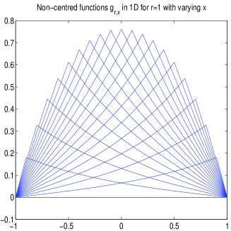
Figure 1: Kernel translates $g_{1,x}$ for the 1D exponential kernel for varying $x$.

Theorem 10.

If $\mathcal{K}=H_{2}^{m}(\mathbb{R}^{d})$, the kernel $K_{r}$ of (10) is the reproducing kernel of the space ${\stackrel{{\scriptstyle\circ}}{{H}}}{}_{2}^{m}(B_{r}(0))$.∎

It is easy to generalize this to smoothly bounded domains $\Omega\subset\mathbb{R}^{d}$ instead of the ball $B_{r}(0)$.

There is a connection to Power Functions on infinite point sets. We can define the Power Function for infinite data outside the ball $B_{r}(0)$ as

$$P_{\|x\|\geq r}(x)=\sup\{v(x)\;:\;\|v\|_{K}\leq 1,v\in V_{r}\}.$$ (11)

Our standard criterion (6) for nonexistence of centralized bump functions now has to be replaced by $V_{r}=\{0\}$, and then the Power Function is zero.

Theorem 11.

In general,

$$P_{\|x\|\geq r}(x)=\|g_{r,x}\|_{K}\hbox{ for all }x\in\mathbb{R}^{d},$$

and if there are bump functions, the supremum in (11) is attained at $g_{r,x}(x)/\|g_{r,x}\|_{K}$. In particular, $P_{\|x\|\geq r}(0)$ is attained at $b_{r}^{*}/\|b_{r}^{*}\|_{K}$, proving

$$P_{\|x\|\geq r}(0)=b_{r}^{*}(0)/\|b_{r}^{*}\|_{K}=\|b_{r}^{*}\|_{K}^{-1}.$$ (12)

Proof.

We assume that there are bump functions. Then $g_{r,x}/\|g_{r,x}\|_{K}$ is admissible, and

$$P_{\|x\|\geq r}(x)\geq g_{r,x}(0)/\|g_{r,x}\|_{K}=\|g_{r,x}\|_{K}.$$

For all $v\in V_{r}$ we have $(v,g_{r,x})_{K}=v(x)$, and therefore

$$|v(x)|\leq\|v\|_{K}\|g_{r,x}\|_{K}$$

proves $P_{\|x\|\geq r}(x)\leq\|g_{r,x}\|_{K}$. In the nonexistence case, all $g_{r,x}$ are zero, like the Power Function. ∎

The relation (12) was observed already in [17] as the extremal situation of a trade-off principle that relates small Power Functions to large norms of bump functions.

Theorem 11 has an interpretation in Spatial Statistics. If a random field $R$ on $\mathbb{R}^{d}$ has observations in all $x$ with $\|x\|_{2}\geq r$,

$$P_{\|x\|\geq r}(0)^{2}=\|b_{r}^{*}\|_{K}^{-2}$$

is the variance of the Kriging predictor, i.e. the best linear unbiased estimator from the data. For Matérn covariances generating $H_{2}^{m}(\mathbb{R}^{d})$, Section 7 has shown that the variance behaves like $r^{2m-d}$. Cases with nonexistence of bump functions are discouraged in Spatial Statistics, because information on an infinite point set like the complement of a ball implies total information.

Again, everything works the same for general domains $\Omega\subset\mathbb{R}^{d}$ with a fixed interior point $x$. One has to project $K(x,\cdot)$ onto

$$V_{\Omega}=\{v\in\mathcal{K}\;:\;v(y)=0\hbox{ for all }y\notin\Omega\}$$

and renormalize the result to be 1 at $x$.

9 Analytic Characterization

Here, we focus on $\mathcal{K}=H_{2}^{m}(\mathbb{R}^{d})$ and want to apply Real Analysis to find more specific results on norm-minimal bump functions, including formulae ready for computational implementation. Since the problem of constructing norm-minimal bump functions can be written as a quadratic optimization with infinitely many constraints in an infinite-dimensional space, there is a variational problem with Lagrange multipliers in the background, but we proceed directly to the constructive solution.

As already stated, the subspace $V_{r}$ of (6) is the closure of $C_{0}^{\infty}(B_{r}(0))$ under the native space norm. In case $\mathcal{K}=H_{2}^{m}(\mathbb{R}^{d})$, it is ${\stackrel{{\scriptstyle\circ}}{{H}}}{}_{2}^{m}(B_{r}(0))$ in standard Sobolev space theory, and the boundary conditions are well-known [16]. By sources on trace theorems, e.g. [20, Thm, 10, Thm. 11], the boundary conditions for embedding ${\stackrel{{\scriptstyle\circ}}{{H}}}{}_{2}^{m}(B_{r}(0))$ into $H_{2}^{m}(\mathbb{R}^{d})$ consist of the classical radial and normal derivatives

$$\gamma_{j,r}=\displaystyle{\frac{\partial^{j}}{\partial\nu^{j}}}|_{\partial B_{r}(0)},\;0\leq j<m-1/2$$

whose extensions map $W_{2}^{m}(B_{r}(0))$ to $W_{2}^{m-j-1/2}(\partial B_{r}(0)),\;0\leq j<m-d/2$. We integrate these over the boundary to define the functionals

$$\lambda_{j,r}(f)=\displaystyle{\int_{\partial B_{r}(0)}\gamma_{j,r}(f)_{|_{x}}dx,,\;0\leq j<m-1/2}$$

and the functions

$$g_{j,r}(x):=\lambda^{y}_{j,r}K(x,y),$$

where $\lambda_{j,r}$ acts on the variable $y$, as indicated by the superscript. These are radial, i.e. rotationally invariant, because the traces of $K(x,\cdot)$ on the boundary just rotate with the direction of $x$, but the integral over the boundary stays the same.

Next, we need the positive definite kernel matrix with entries

$$\lambda^{x}_{k,r}\lambda^{y}_{j,r}K(x,y)=\lambda^{x}_{k,r}g_{j,r}(x),\;0\leq j,k<m-1/2$$

and solve the $r$-dependent linear system

$$g_{k,r}(0)=\lambda^{y}_{k,r}K(y,0)=\displaystyle{\sum_{j=0}^{j<m-1/2}c_{j}(r)\lambda^{x}_{k,r}\lambda^{y}_{j,r}K(x,y)},\;0\leq k<m-1/2$$ (13)

for functions $c_{j}(r),\;0\leq j<m-1/2$.

Theorem 12.

Norm-minimal compactly supported functions $b_{r}^{*}$ for Sobolev spaces $H_{2}^{m}(\mathbb{R}^{d})$ can be calculated via the radial function

$$g_{r}(y):=K(0,y)-\displaystyle{\sum_{j=0}^{j<m-1/2}c_{j}(r)g_{j,r}(y)}$$ (14)

in the above way, finally using (7).

Proof.

By Theorem 9 of Section 8, we need the projection $P_{{\stackrel{{\scriptstyle\circ}}{{H}}}{}_{2}^{m}(B_{r}(0))}$ in $H_{2}^{m}(\mathbb{R}^{d})$ onto ${\stackrel{{\scriptstyle\circ}}{{H}}}{}_{2}^{m}(B_{r}(0))$ and the function

$$g_{r}(\cdot)=P_{{\stackrel{{\scriptstyle\circ}}{{H}}}{}_{2}^{m}(B_{r}(0))}K(0,\cdot)$$

which is $b_{r}^{*}$ up to a factor by $b_{r}^{*}(x)=g_{r}(x)/g_{r}(0)$. Due to (9), the necessary and sufficient optimality conditions are $g_{r}\in{\stackrel{{\scriptstyle\circ}}{{H}}}{}_{2}^{m}(B_{r}(0))$ and

$$\begin{array}[]{rcl}(K(0,\cdot)-g_{r},v_{r})_{H_{2}^{m}(\mathbb{R}^{d})}&=&0\end{array}$$

$\hbox{ for all }r\in V_{r}={\stackrel{{\scriptstyle\circ}}{{H}}}{}_{2}^{m}(B_{r}(0))$. But (14) implies

$$\begin{array}[]{rcl}(K(0,\cdot)-g_{r},v_{r})_{H_{2}^{m}(\mathbb{R}^{d})}&=&\displaystyle{\left(\sum_{j=0}^{j<m-1/2}c_{j}(r)g_{j,r},v_{r}\right)_{H_{2}^{m}(\mathbb{R}^{d})}}\\ &=&\displaystyle{\sum_{j=0}^{j<m-1/2}c_{j}(r)(g_{j,r},v_{r})_{H_{2}^{m}(\mathbb{R}^{d})}}\\ &=&\displaystyle{\sum_{j=0}^{j<m-1/2}c_{j}(r)(\lambda^{y}_{j,r}K(\cdot,y),v_{r})_{H_{2}^{m}(\mathbb{R}^{d})}}\\ &=&\displaystyle{\sum_{j=0}^{j<m-1/2}c_{j}(r)\lambda^{y}_{j,r}v_{r}(y)}\\ &=&0\hbox{ for all }v_{r}\in V_{r}.\end{array}$$

The system (13) is the same as

$$\lambda^{y}_{k,r}g_{r}(y)=0,\;0\leq k<m-1/2,$$

but since $g_{r}$ is radial, the boundary values and radial derivatives are constant and therefore zero. ∎

This seems to be the first case handling infinitely many data with infinitely many kernel translates, in this case placed on the $r$-sphere and treated in a rotationally symmetric way. The definition of the functions $g_{j,r}$ cares for orthogonality to $V_{r}$ and involves all of these translates fairly. The linear system (13) has a different purpose: it cares for the correct smoothness of the result on the boundary. If the $g_{j,r}$ and their derivatives are calculated on the boundary with sufficient accuracy, the system can be set up and solved like any other Hermite interpolation.

For domains $\Omega$ with a fixed interior point, the proof logic stays the same, but the radiality arguments fail. Everything works as long as the trace theorems are valid, but this fails for pathological subdomains.

We add a remark on the background, connected to the old theory of $L$-splines [18]. The inner product $(f,g)_{K}$ can be written as $(Lf,Lg)_{L_{2}(\mathbb{R}^{d})}$ for a pseudodifferential operator $L\;:\;\mathcal{K}\to L_{2}(\mathbb{R}^{d})$ defined by

$$\widehat{Lf}(\omega)=\hat{f}(\omega)\sqrt{\hat{K}(\omega)}.$$

Then the reproduction equation $f(x)=(f,K(x,\cdot))_{K}=(Lf,LK(\cdot,x))_{L_{2}(\Omega)}$ is a way to define that $(L^{*}L)^{y}K(y,x)=\delta_{x}$ holds for all $x\in\mathbb{R}^{d}$, i.e. the kernel is a fundamental solution. In the Sobolev case $H_{2}^{m}(\mathbb{R}^{d})$, the operator $L^{*}L$ is the classical elliptic differential operator $(Id-\Delta)^{m}$. Compactly supported functions on a smooth domain $\Omega$ must then obey the boundary conditions for the Dirichlet problem for $L^{*}L$ on $\Omega$ with zero boundary conditions. Consequently, bump functions may already be present in the literature on elliptic PDE problems. Anyway, they are possibly useful in the Method of Fundamental Solutions [2, 4].

10 Examples

We first consider the simplest Sobolev space $H_{2}^{m}(\mathbb{R}^{d})$ for $m=1=d$ with the radial exponential kernel $K(x,y)=\exp(-|x-y|)$. Then the functional

$$\lambda_{0,r}(v)=v(-r)+v(r)\hbox{ for all }v\in W_{2}^{1}(\mathbb{R}^{1})$$

“integrates” over the trace operator $T(v)=(v(r),v(-r))\in\mathbb{R}^{2}$. With some explicit calculations omitted,

$$\begin{array}[]{rcl}g_{0,r}(x)&=&\displaystyle{\exp(-|r-x|)+\exp(-|-r-x|)}\\ g_{r}(x)&=&\exp(-|x|)-c_{0}\displaystyle{(\exp(-|r-x|)+\exp(-|-r-x|)}\\ c_{0}(r)&=&\displaystyle{\frac{1}{\cosh(r)}}\\ g_{r}(x)&=&\displaystyle{\frac{\sinh(r-|x|)}{\cosh(r)}}\\ b_{r}^{*}(x)&=&\displaystyle{\frac{g_{r}(x)}{g_{r}(0)}}=\displaystyle{\frac{\sinh(r-|x|)}{\sinh(r)}}\end{array}$$

where the third equation follows somewhat easier from setting $g_{r}(x)=0$ for $x=\pm r$. This is the situation of Figure 2. The corresponding general kernel translates in the sense of (10) are in Figure 1, obtained via projection of $K(x,\cdot)$ instead of $K(0,\cdot)$.

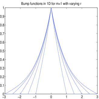
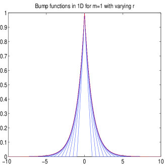
Figure 2: Bump functions for the 1D exponential kernel for varying $r$. Left: $r=1,\,1.5,\,2,\,2.5,\,3$, right: $r=1,\ldots,50$. The red line is the kernel $K(0,y)=\exp(-|y|)$ occurring numerically in the limit.

The same kernel works for all cases with $2m-d=1$, but things get much more difficult for $d>1$, because we now have to integrate over circles, using

$$\lambda_{0,r}(f)=\displaystyle{\int_{0}^{2\pi}f(r\cos\varphi+r\sin(\varphi))d\varphi.}$$

To keep things simpler, we shall use radiality whenever possible.

We first consider $d=2,\,m=3/2$ and set $x=r(\cos(\varphi),\sin(\varphi))$ and $z=(1,0)$ to get

$$\|x-tz\|^{2}=(r\cos(\varphi)-t)^{2}+(r\sin(\varphi))^{2}$$ (15)

and

$$\begin{array}[]{rcl}g_{0,r}(tz)&=&\displaystyle{\int_{0}^{2\pi}\exp\left(-\sqrt{(r\cos(\varphi)-t)^{2}+(r\sin(\varphi))^{2}}\right)d\varphi}\\ &=&\displaystyle{\int_{0}^{2\pi}\exp\left(-\sqrt{r^{2}+t^{2}-2r|t|\cos(\varphi)}\right)d\varphi}\end{array}$$

because the cases $t$ and $-t$ have the same trace on the circle. The ingredients for (13) are $g_{0,r}(0)=2\pi\exp(-r)$ and

$$\lambda^{x}_{0,r}\lambda^{y}_{0,r}K(x,y)=\lambda^{x}_{0,r}g_{0,r}(x)=2\pi g_{0,r}(rz)$$

because $g_{0,r}$ is constant on the boundary and equal to $g_{0,r}(rz)$. Therefore

$$c_{0}(r)=\displaystyle{\frac{\exp(-r)}{g_{0,r}(rz)}}$$

and we get

$$g_{r}(x)=\exp(-\|x\|_{2})-\displaystyle{\frac{\exp(-r)g_{0,r}(x)}{g_{0,r}(rz)}}.$$

Figure 3 shows the norm-minimal bump functions (solid) in the 1D (blue) and 2D case (red). The 2D case has a vanishing derivative at zero, visible by zooming in, but still just continuity at $r$. But note that functions in $W_{2}^{3/2}(\mathbb{R}^{2})$ are only continuous, not continuously differentiable. For comparison, the Wendland functions are added as dashed lines. It is remarkable that in the 2D case the Wendland functions have derivative discontinuities at zero, while the bump functions have them at $r$. In case $r=10$, the exponential decay of bump functions is apparent, while Wendland functions decay polynomially. Smaller $r$ behave much like scaled versions of the case $r=1$.

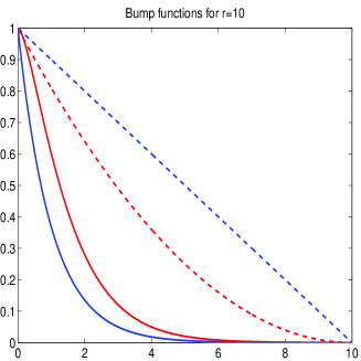
Figure 3: Bump functions (solid) for the exponential kernel, $r=1$ (left) and $r=10$ (right). The red curves are for $W_{2}^{3/2}(\mathbb{R}^{2})$, the blue curves for $W_{2}^{1}(\mathbb{R}^{1})$. The corresponding Wendland functions are dashed.

Staying in the bivariate setting with larger $m$ just uses different kernels, but now we get the linear system (13) to solve. If we want a derivative condition in $\mathbb{R}^{2}$, we can take $m=2.5$ or $m=2$. When examining the case $m=2$, the function $g_{1,r}$ has a singularity at the boundary, due to nonexistence of second derivatives in $W_{2}^{2}(\mathbb{R}^{2})$. For $m=2.5$, results are in Figure 4. The corresponding Wendland function $\phi_{3,1}(t)=(1-t/r)_{+}^{4}(1+4t/r)$ is in $C^{2}$ and vanishes of third order at $r$. The norm-minimal compactly supported function seems to have the same smoothness at zero and at the boundary.

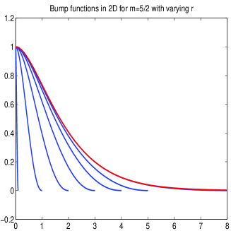
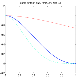
Figure 4: Left: optimal bump functions for the 2D exponential kernel for $W_{2}^{5/2}(\mathbb{R}^{2})$ with varying $r$. The red line is the normalized kernel occurring in the limit. Right: the case $r=1$ with the Wendland function $\phi_{3,1}$ in cyan and dashed.

11 Summary, Conclusions, and Open Problems

For a given support radius $r$, each Sobolev space $H_{2}^{m}(\mathbb{R}^{d})$ with $m>d/2$ has a unique “bump” function with minimal norm, value 1 at the origin and vanishing outside the interior of the ball $B_{r}(0)$ with radius $r$ around the origin. Under all compactly supported functions with norm up to one and value one at the origin, it has smallest support. And under all functions with support in $B_{r}(0)$ with norm up to one, they attain the maximum value at zero, up to a factor.

Such functions are an intrinsic and characteristic feature of the space and could be called $S$-splines.

They are radial, and their radial univariate profile can be precalculated to high accuracy by the construction of Section 9. By the results on scaling in Section 7, they can be downscaled to smaller support radii, at asymptotically no loss. There are connections to upper bounds of convergence rates of kernel-based interpolation, because they are Power Functions for data outside a given ball. In Spatial Statistics using random fields with Matérn kernels, they give the variance for Kriging estimation at zero provided that there is full information outside the $r$-ball.

In Hilbert space terms, these functions are obtainable by renormalization of the projection of the reproducing kernel in $H_{2}^{m}(\mathbb{R}^{d})$ onto ${\stackrel{{\scriptstyle\circ}}{{H}}}{}_{2}^{m}(B_{r}(0))$. In terms of Real Analysis, they are computable by applying the trace operator to the reproducing kernel under radial symmetry.

For interpolation or approximation in Sobolev spaces, their translates provide a compactly supported radial basis, leading to sparse matrices, but there are no results yet on linear independence or positive definiteness. In particular, their Fourier transforms are not yet known, but they must have an optimality property as well. The functions seem to be bell-shaped [8] and pointwise decreasing for increasing $r$, but this is still open. For use in meshless methods for PDE solving, they are shape functions [1] that deserve further investigation. Finally, they may lead to new multivariate wavelet constructions, like many other compactly supported functions.

To make the numerical application of optimal compactly supported functions easier, a follow-up paper should publish the radial profiles in full computational accuracy. This opens the way to various sparse meshless methods for interpolation, approximation, and PDE solving. Then it is interesting to see how much bandwidth is needed to let them work at maximal possible convergence rate.

The results of this paper should generalize to any kernel-based Hilbert space with limited smoothness, and hopefully also to Beppo-Levi spaces generated by conditionally positive definite kernels. Also, the restriction to balls centred around the origin is easy to overcome, losing radiality arguments. Then it is interesting to construct them on tilings of the space, like finite elements. Their superposition will stay in Sobolev space because of zero boundary conditions.

Final Remarks

There was no funding except the standard retirement program for professors in the state of Lower Saxony, Germany.

This work would not have been possible without the long-term friendship with Elisabeth Larsson (Uppsala) and Oleg Davydov (Gießen), leading to publications [10, 6]. Bump functions were a central tool in these papers.

References

• [1] T. Belytschko, Y. Krongauz, D.J. Organ, M. Fleming, and P. Krysl. Meshless methods: an overview and recent developments. Computer Methods in Applied Mechanics and Engineering, special issue, 139:3–47, 1996.
• [2] A. Bogomolny. Fundamental solutions method for elliptic boundary value problems. SIAM J. Numer. Anal., 22:644–669, 1985.
• [3] M.D. Buhmann. Radial Basis Functions, Theory and Implementations. Cambridge University Press, Cambridge,UK, 2003.
• [4] C.S. Chen, A. Karageorghis, and Y.S. Smyrlis. The Method of Fundamental Solutions - A Meshless Method. Dynamic Publishers, 2008.
• [5] O. Davydov and R. Schaback. Error bounds for kernel-based numerical differentiation. Numerische Mathematik, 132:243–269, 2016.
• [6] O. Davydov and R. Schaback. Optimal stencils in Sobolev spaces. IMA Journal of Numerical Analysis, 39:398–422, 2019.
• [7] St. De Marchi and R. Schaback. Stability of kernel-based interpolation. Adv. in Comp. Math., 32:155–161, 2010.
• [8] N. Dyn and D. Levin. Bell–shaped basis functions for surface fitting. In Z. Ziegler, editor, Approximation Theory and Applications, pages 113–129. Academic Press, 1981.
• [9] G. Fasshauer and M. McCourt. Kernel-based Approximation Methods using MATLAB, volume 19 of Interdisciplinary Mathematical Sciences. World Scientific, Singapore, 2015.
• [10] E. Larsson and R. Schaback. Scaling of radial basis functions. IMA Journal of Numerical Analysis, 2023.
• [11] F.J. Narcowich, J.D. Ward, and H. Wendland. Sobolev error estimates and a Bernstein inequality for scattered data interpolation via radial basis functions. Constructive Approximation, 24:175–186, 2006.
• [12] Emilio Porcu, Moreno Bevilacqua, Robert Schaback, and Chris J. Oates. The matérn model: A journey through statistics, numerical analysis and machine learning. Statist. Sci., 39(3):469–492, 2024.
• [13] R. Schaback. Error estimates and condition numbers for radial basis function interpolation. Advances in Computational Mathematics, 3:251–264, 1995.
• [14] R. Schaback. On the efficiency of interpolation by radial basis functions. In A. LeMéhauté, C. Rabut, and L.L. Schumaker, editors, Surface Fitting and Multiresolution Methods, pages 309–318. Vanderbilt University Press, Nashville, TN, 1997.
• [15] R. Schaback. The missing Wendland functions. Advances in Computational Mathematics, 43:76–81, 2010.
• [16] R. Schaback. Superconvergence of kernel-based interpolation. Journal of Approximation Theory, 235:1–19, 2018.
• [17] R. Schaback. Small errors imply large evaluation instabilities. Advances in Computational Mathematics, 49:49:25, 2023.
• [18] M.H. Schultz and R.S. Varga. $L$-splines. Numerische Mathematik, 10:345–369, 1967.
• [19] B.V. Shabat. Introduction to Complex Analysis: Functions of Several Variables. Translations of Mathematical Monographs. American Mathematical Society, 1976.
• [20] Tatyana Suslina. Sobolev spaces. Technical report, Universität Stuttgart, Lecture Note, 2024. https://pnp.mathematik.uni-stuttgart.de/iadm/Weidl/fa-ws04/Suslina_Sobolevraeume.pdf.
• [21] H. Wendland. Piecewise polynomial, positive definite and compactly supported radial functions of minimal degree. Advances in Computational Mathematics, 4:389–396, 1995.
• [22] H. Wendland. Scattered Data Approximation. Cambridge University Press, Cambridge,UK, 2005.
• [23] B. Zwicknagl. Power series kernels. Constructive Approximation, 29(1):61–84, 2009.
• [24] B. Zwicknagl and R. Schaback. Interpolation and approximation in Taylor spaces. Journal of Approximation Theory, 171:65–83, 2013.