New solutions of the Poincaré Center Problem in degree 3

Abstract.

Let $\omega$ be a plane autonomous system and $C$ its configuration of algebraic integral curves. If the singularities of $C$ are quasi homogeneous we give new conditions for existence of a Darboux first integral. This is used to construct new components of the center variety in degree 3.

1. Introduction

In 1885 Poincaré [Poi85] asked when the differential equation

$$y^{\prime}=-\frac{x+p(x,y)}{y+q(x,y)}=:-\frac{P(x,y)}{Q(x,y)}$$

with convergent power series $p(x,y)$ and $q(x,y)$ starting with quadratic terms, has stable solutions in the neighborhood of the equilibrium solution $(x,y)=(0,0)$. This means that in such a neighborhood the solutions of the equivalent plane autonomous system

$$\dot{x} =y+q(x,y)=Q(x,y)$$

$$\dot{y} =-x-p(x,y)=-P(x,y)$$

are closed curves around $(0,0)$. We say, that such an differential equation has a center at $(0,0)$.

Poincaré showed that one can iteratively find a formal power series $F=x^{2}+y^{2}+f_{3}(x,y)+f_{4}(x,y)+\dots$ such that

$$\det\begin{pmatrix}F_{x}&F_{y}\\ P&Q\end{pmatrix}=\sum_{j=1}^{\infty}s_{j}(x^{2j+2}+y^{2j+2})$$

with $s_{j}$ rational polynomials in the coefficients of $P$ and $Q$. If all $s_{j}$ vanish, and $F$ is convergent then $F$ is a constant of motion, i.e. its gradient field satisfies $Pdx+Qdy=0$. Since $F$ starts with $x^{2}+y^{2}$ this shows that close to the origin all integral curves are closed and the system is stable. Therefore the $s_{j}$’s are called the focal values of $Pdx+Qdy$. Often also the notation $\eta_{2j}:=s_{j}$ is used, and the $\eta_{i}$ are called Lyapunov quantities.

Poincaré also showed that if an analytic constant of motion exists, the focal values must vanish. Later Frommer [Fro34] proved that the systems above are stable if and only if all focal values vanish even without the assumption of convergence of $F$. (Frommer’s proof contains a gap which can be closed [vW05].)

Unfortunately it is in general impossible to check Poincaré’s condition for a given differential equation because there are infinitely many focal values. In the case where $P$ and $Q$ are polynomials of degree at most $d$, the $s_{j}$ are polynomials in finitely many unknowns. Hilbert’s Basis Theorem then implies that the ideal $I_{\infty}=(s_{1},s_{2},\dots)$ is finitely generated and that the solution set is an algebraic variety, the center variety.

Poincaré was inspired by work of Darboux [Dar78] who showed that the existence of algebraic integral curves often implies the existence of a constant of motion. Such systems are now called Darboux integrable. We review Darboux’s Theorem in Section 2.

For $d=2$ the center variety has $4$ components and each component is characterized by a certain type of algebraic integral curve configuration:

1. three lines in general position

2. a line and a conic in general position

3. infinitely many cubics

4. a conic and a cubic in special position.

All these differential forms are Darboux integrable with respect to the given curve configuration. [Dul08]

In degree $3$ a new type of center appears, the rational reversible centers. These have been classified by Żoła̧dek [Żoł94]. On the other hand the classification of Darboux centers in degree $3$ is still open and seems very difficult. So for $d=3$ only partial results are known, for example [CRŻ97] and [Chr05]. In [Żoł96] Żoła̧dek gives a list of $52$ families of differential forms known to have centers. $35$ of these are Darboux integrable. In [vBK10] we analyze which of Żoła̧dek’s families form reduced components of the center variety (22 of the 52). The other ones either give non reduced components or are proper subfamilies of reduced components.

Computer experiments over finite fields [vBK10], [Ste11] seem to indicate that Żoła̧dek’s list is complete up to codimension $8$ and that for higher codimension more than $100$ additional components exist. It is the aim of this paper to present a geometric construction for some of these components and give a rigorous proof of their existence over $\mathbb{C}$.

Our method is a refinement of Darboux’ ideas, incorporating curve configurations in special position with simple singularities. This has two parts:

Firstly, for a given curve configuration we have to describe the vector space of differential forms having the given curve configuration among their integral curves. This is called the inverse problem by Christopher, Llibre and Pantazi in [CLPW12]. We use the Tjuringa number from singularity theory for our estimate. This is done in Section 3.

Secondly we would like to prove Darboux integrability for a differential form $\omega$ with a given curve configuration among its integral curves. For this we evaluate the cofactors of the integral curves and $d\omega$ at the singular points. We prove that for simple singularities the ratio of these values depends solely on the type of the singularity (and not on $\omega$). Using these ratios we find special linear combinations of cofactors and $d\omega$ for which we can apply Darboux’ Theorem. These ideas are developed in Section 4.

Finally, in Section 5 we use our methods to construct new components of the $d=3$ center variety in codimension $9$. We found the special curve configurations used for these constructions by analyzing data obtained from computer experiments over a finite field [vBK10], [Ste11].

2. Preliminaries

In this article we describe a plane autonomous system by a differential form $\omega=P\operatorname{dx}+Q\operatorname{dy}$ with polynomial coefficients $P,Q\in\mathbb{C}[x,y]$ of degree at most $d$.

Definition 2.1.

Let $\omega$ be a differential form and $F,\mu\in\mathbb{C}[[x,y]]$ power series. If

$$dF=\mu\omega$$

then $F$ is called a first integral and $\mu$ a cofactor of $\omega$

For a given $\omega$ it can often be very difficult to decide, whether a first integral exists. Darboux realized in 1878 that the existence of algebraic integral curves can help to answer this question:

Definition 2.2.

Let $C\in\mathbb{C}[x,y]$ be a polynomial and $C=0$ the plane algebraic curve defined by $C$. $C=0$ is called an algebraic integral curve of a differential $\omega$ if and only if

$$dC\wedge\omega|_{C}=0\iff dC\wedge\omega=C\cdot K_{C}$$

In this situation the $2$-form $K_{C}$ is called the cofactor of $C$. In a slight abuse of notation we sometimes also denote the algebraic curve $\{C=0\}$ by the letter $C$.

Theorem 2.3 (Darboux 1878).

Let $\omega$ be a plane autonomous system, $C_{1},\dots,C_{r}$ algebraic integral curves of $\omega$ and $K_{1},\dots,K_{r}$ their cofactors.

• If $\sum\alpha_{i}K_{i}=-d\omega$ for appropriate $\alpha_{i}\in\mathbb{C}$ then $\mu=\prod C_{i}^{\alpha_{i}}$ is an integrating factor of $\omega$.

• If $\sum\alpha_{i}K_{i}=0$ for appropriate $\alpha_{i}\in\mathbb{C}$ then $F=\prod C_{i}^{\alpha_{i}}$ is a first integral of $\omega$.

Proof.

For the first claim calculate:

$$d(\mu\omega) =d\mu\wedge\omega+\mu d\omega$$

$$=\mu\bigl{(}\frac{d\mu}{\mu}\wedge\omega+d\omega\bigr{)}$$

$$=\mu(d\log\mu\wedge\omega+d\omega)$$

$$=\mu\bigl{(}\sum\alpha_{i}d\log C_{i}\wedge\omega+d\omega\bigr{)}$$

$$=\mu\bigl{(}\sum\alpha_{i}\frac{dC_{i}}{C_{i}}\wedge\omega+d\omega\bigr{)}$$

$$=\mu\bigl{(}\sum\alpha_{i}K_{i}+d\omega\bigr{)}$$

$$=0$$

consequently there exists an $F$ with $dF=\mu\omega$.

For the second claim we observe that

$$dF=\mu\omega\iff dF\wedge\omega=0.$$

We then have a similar computation:

$$dF\wedge\omega =F\Bigl{(}\frac{dF}{F}\wedge\omega\Bigr{)}$$

$$=F(d\log F\wedge\omega)$$

$$=F\sum\alpha_{i}d\log C_{i}\wedge\omega$$

$$=F\sum\alpha_{i}K_{i}$$

$$=0$$

∎

Sometimes the following trivial observation is useful

Lemma 2.4.

Let $C,D$ be plane algebraic curves without common components and $\omega$ a differential from Then $C$ and $D$ are integral curves of $\omega$ if and only if $C\cup D$ is.

Proof.

The integral curve condition can be checked locally outside the intersection points of $C$ and $D$. Since this is a closed condition, it is enough to check it on an open dense subset on each component. ∎

In this paper we will consider singular algebraic integral curves. For this we recall some singularity theory of plane algebraic curves. For a detailed introduction, see [GLS07].

Definition 2.5.

Let $F\in\mathbb{C}[[x,y]]$ be the germ of a singularity at $0$. Then

$$m=\dim\frac{\mathbb{C}[[x,y]]}{(F_{x},F_{y})}$$

is called the Milnor number of $F$. Similarly

$$t=\dim\frac{\mathbb{C}[[x,y]]}{(F_{x},F_{y},F)}Similarly$$

is called the Tjurina number of $F$. Notice that $m\geq t$ with equality for quasi homogeneous singularities.

Example 2.6.

The so called simple singularities are

name	local equation	$m=t=c$
node ($A_{1}$)	$x^{2}-y^{2}$	1
cusp ($A_{2}$)	$x^{2}-y^{3}$	2
tacnode ($A_{3}$)	$x^{2}-y^{4}$	3
$A_{n}$	$x^{2}-y^{n+1}$	n
triple point ($D_{4}$)	$x^{3}-y^{3}$	4
$D_{n}$	$y(x^{2}-y^{n-2})$	n
$E_{6}$	$x^{3}-y^{4}$	6
$E_{7}$	$x(x^{2}-y^{3})$	7
$E_{8}$	$x^{3}-y^{5}$	8

The simple singularities are all quasi homogeneous and therefore $m=t$. Furthermore for simple singularities the maximum number of conditions $c$ a polynomial must satisfy to ensure that it has a singularity of this type is also equal to the Milnor number.

In addition to the simple singularities, we also need four-fold points which have a local equation $x^{4}+\alpha x^{2}y^{2}+y^{4}$ with arbitrary $\alpha$. They have $m=t=9$.

We will also consider special points at infinity. Here the conditions appearing in the center focus setting do not match those in singularity theory.

Proposition 2.7.

Let $C\in\mathbb{C}[x,y,z]$ be a homogeneous polynomial of degree $d$ and $C^{\prime}\in\mathbb{C}[x,z]$ its dehomogenization with respect to $y$. Consider the grading $\deg x=b$ and $\deg y=a$ on $\mathbb{C}[x,z]$ and assume further that

$$C^{\prime}=x^{a}+z^{b}+\text{ terms of $\deg>ab$.}$$

Let $X=V(C_{x},C_{y},C)$ and assume furthermore that $ab\leq 2a+b$. Then $\deg X=(a-1)b$.

Proof.

Since $C$ is homogeneous of degree d we have $C=(1/d)(xC_{x}+yC_{x}+zC_{z})$ and the Darboux Ideal is

$$I=(C_{x},C_{y},C)=(C_{x},C_{y},zC_{z})$$

We have

$$C=y^{d-a}x^{a}+y^{d-b}z^{b}+\text{higher order terms}$$

and

$$C_{y}=(d-a)y^{d-a-1}x^{a}+(d-b)y^{d-b-1}z^{b}+\text{higher order terms}.$$

Dehomogenization with respect to $y$ gives

$$C_{y}^{\prime}=(d-a)x^{a}+(d-b)z^{b}+\text{higher order terms}.$$

For the other variables we calculate directly

$$C_{x}^{\prime} =ax^{a-1}+\text{higher order terms}$$

$$zC_{z}^{\prime} =bz^{b}+\text{higher order terms}.$$

It follows that the initial ideal of $I$ contains $x^{a-1}$ and $z^{b}$. Further initial terms can only come from reducing $C_{y}^{\prime}$ modulo $C_{x}^{\prime}$ and $zC_{z}^{\prime}$:

$$C_{y}^{\prime}-\frac{d-a}{a}xC_{x}-\frac{d-b}{b}zC_{z}^{\prime}$$

has only terms of weighted degree at least $ab+1$. We claim that all these terms are divisible either by $x^{a-1}$ or $z^{b}$. Assume that this is not true. Then each term has degree at most $(a-2)$ in $x$ and at most $(b-1)$ in $z$. Consequently all terms have weighted degree at most

$$b(a-2)+a(b-1)=2ab-a-2b\leq ab$$

by assumption. But this contradicts that all terms have degree at least $ab+1$. Therefore all terms must be divisible by either $x^{a-1}$ or $z^{b}$ and no further initial terms can occur. It follows that

$$\deg X=\deg V(x^{a-1},z^{b})=(a-1)b.$$

∎

Example 2.8.

We will be interested in the following cases:

name	equation $C^{\prime}$	$t$
tangent to line at $\infty$	$(z+x^{2})+\dots$	1
general node at $\infty$	$(z^{2}+x^{2})+\dots$	2
general triple point at $\infty$	$(z^{3}+x^{3})+\dots$	6
node at $\infty$ with one branch	$xz+\dots$	$\geq 3$
tangent to the line at $\infty$

Here $t$ is the degree of $X=V(C_{x},C_{y},C)$ at $(0:1:0)$.

The first three follow from Proposition 2.7. For the fourth we assume in addition that $\deg V(C_{x},C_{y},C)$ is finite at $(0:1:0)$ and make a similar computation:

$$C_{x}^{\prime} =z+\text{higher order terms}$$

$$C_{y}^{\prime} =(d-2)zx+\text{higher order terms}$$

$$zC_{z}^{\prime} =zx+\text{higher order terms}$$

We see initial terms $z$ and $zx$ directly. New initial terms can occur in the following $3$ polynomials

$$C_{z}^{\prime}-(d-2)xC_{x}^{\prime} C_{y}^{\prime}-(d-2)zC_{z}^{\prime} xC_{x}^{\prime}-xC_{z}^{\prime}$$, and .

Since $\deg V(C_{x},C_{y},C)$ is finite, the initial ideal must also contain a monomial of the form $x^{k}$. Since all therms of the polynomials above are of degree $3$ and larger we conclude that $k\geq 3$ and therefore $t\geq 3$. For generic higher order terms we get $t=3$.

3. The inverse problem

For a given configuration of algebraic curves we would like to determine the vector space of degree $d$ differential forms that have this configuration as an integral curve. This is called the inverse problem by Christopher, Llibre and Pantazi in [CLPW12].

Definition 3.1.

If $P\in\mathbb{C}[x,y]$ is a polynomial of degree $d$, we denote by $\overline{P}\in\mathbb{C}[x,y,z]$ its homogenization. For differential forms $\omega=P\operatorname{dx}+Q\operatorname{dy}$ we define $\overline{\omega}:=\overline{P}dx+\overline{Q}dy$.

Remark 3.2.

Notice that the definition of algebraic integral curves and cofactors do not change if we homogenize everything. Similarly Darboux’ Theorem also holds for homogenized polynomials.

Definition 3.3.

Let $C_{1},\dots,C_{r}\in\mathbb{C}[x,y,z]$ be homogeneous polynomials of degree $e_{i}$. Then

$$\begin{pmatrix}C_{1x}&C_{1y}&C_{1}&&\\ \vdots&\vdots&&\ddots&\\ C_{rx}&C_{ry}&&&C_{r}\end{pmatrix}$$

is called the Darboux Marix of the configuration $C_{i}$.

Proposition 3.4.

Let $C_{i},\dots,C_{r}$ be a configuration of plane curves. A differential from $\omega=P\operatorname{dx}+Q\operatorname{dy}$ has integral curves $C_{i}$ with cofactors $K_{i}\operatorname{dx}\operatorname{dy}$ if and only if

$$M\cdot(Q,-P,-K_{1},\dots,-K_{r})^{t}=0$$

where $M$ is the Darboux matrix of $C_{i}$.

Proof.

The definition of integral curve gives

$$0 =dC_{i}\wedge\omega-C_{i}K_{i}\operatorname{dx}\operatorname{dy}$$

$$=(C_{ix}\operatorname{dx}+C_{iy}\operatorname{dy})\wedge(P\operatorname{dx}+Q\operatorname{dy})-C_{i}K_{i}\operatorname{dx}\operatorname{dy}$$

$$=(C_{ix}Q-C_{iy}P-C_{i}K_{i})\operatorname{dx}\operatorname{dy}.$$

Writing these equations in matrix form gives the claimed identity. ∎

Corollary 3.5.

Let $C_{i},\dots,C_{r}$ be a configuration of plane curves of degree $e_{i}$ , and consider the morphism of vector bundles

$$2{\mathcal{O}}\oplus r{\mathcal{O}}(-1)\xrightarrow{\phi_{M}}\bigoplus{\mathcal{O}}(e_{i}-1)$$

defined by the Darboux matrix $M$ of the $C_{i}$. Then the vector space of degree $d$ differential forms that have the $C_{i}$ as integral curves is

$$H^{0}(\ker\phi_{M}(d)).$$

Proof.

This is just the sheafification of Proposition 3.4. ∎

We now want to calculate the dimension of this vector space. Because of Lemma 2.4 is is enough to consider the case of one (possibly very singular and reducible) integral curve $C$.

Proposition 3.6.

Let $C$ be a plane curve of degree $e$, $I=(C_{x},C_{y},C)$ the ideal defined by the entries of the Darboux matrix of $C$ and $X\subset\mathbb{P}^{2}$ the scheme defined by $I$. If $\dim X=0$ and $h^{1}({\mathcal{I}}(d+e-1))=0$ then

$$h^{0}(\ker\phi_{M}(d))\geq 2{d+2\choose 2}+{d+1\choose 2}-{d+e+1\choose 2}+\deg X=:\eta.$$

We call $\eta$ the expected number of differential forms with configuration $C$ integral curves.

Proof.

Consider the exact sequence

$$0\to\ker\phi_{M}(d)\to 2{\mathcal{O}}(d)\oplus{\mathcal{O}}(d-1)\to{\mathcal{O}}(d+e-1)\to\operatorname{coker}\phi_{M}(d)\to 0.$$

Since $X$ is defined by the vanishing of the entries of $M$ we have $\operatorname{coker}\phi_{M}={\mathcal{O}}_{X}$. By the additivity of $\chi$ we obtain

$$\chi(\ker\phi_{M}(d)) =2\chi({\mathcal{O}}(d))+\chi({\mathcal{O}}(d-1))-\chi({\mathcal{O}}(d+e-1))+\chi({\mathcal{O}}_{X})$$

$$=2{d+2\choose 2}+{d+1\choose 2}-{d+e+1\choose 2}+\deg X$$

Now

$$\chi(\ker\phi_{M}(d))=h^{0}(\ker\phi_{M}(d))-h^{1}(\ker\phi_{M}(d))+h^{2}(\ker\phi_{M}(d))$$

by definition. Since $h^{1}$ is always positive, the claim follows if $h^{2}=0$.

For this let ${\mathcal{I}}$ be the sheafification of $I$. We then have two short exact sequences

$$0\to{\mathcal{I}}(d+e-1)\to{\mathcal{O}}(d+e-1)\to{\mathcal{O}}_{X}\to 0$$

and

$$0\to\ker\phi_{M}(d)\to 2{\mathcal{O}}(d)\oplus{\mathcal{O}}(d-1)\to{\mathcal{I}}(d+e-1)\to 0.$$

Since $d$ is positive, ${\mathcal{O}}(d)$ and ${\mathcal{O}}(d-1)$ have no higher cohomology. Therefore the long exact cohomology sequence of the second short exact sequence gives

$$h^{2}(\ker\phi_{M}(d))=h^{1}({\mathcal{I}}(d+e-1))$$

and $h^{1}({\mathcal{I}}(d+e-1))=0$ by assumption. ∎

We now want to consider this construction in families. For this let $B$ be an irreducible smooth quasi projective variety and

an algebraic family of plane curves given by a section

$${\mathcal{O}}_{B\times\mathbb{P}^{2}}\xrightarrow{C}\pi^{*}({\mathcal{O}}(e)).$$

The Darboux construction gives a morphism of vector bundles

$$2{\mathcal{O}}\oplus r{\mathcal{O}}(-1)\xrightarrow{\phi}\bigoplus{\mathcal{O}}(e-1).$$

The cokernel of $\phi$ is ${\mathcal{O}}_{X}$ for a family of schemes $X$:

Proposition 3.7.

Consider a family of curve configurations as above. Assume that $\pi_{X}\colon X\to B$ is finite and $\deg X_{b}\geq k$ for all $b\in B$.

If there exists a point $0\in B$ such that

1. $\deg X_{0}=k$

2. $h^{1}({\mathcal{I}}_{X_{0}}(d+e-1))=0$

3. $h^{0}(\ker\phi_{M_{0}}(d))=\eta\geq 0$ as expected,

then there exists a rank $\eta$ vector bundle ${\mathcal{E}}$ on an open subset $B^{\prime\prime}\subset B$ such that $\mathbb{P}({\mathcal{E}})$ parametrizes differential forms of degree $d$ whose configuration of integral curves contains $C_{b}$ for an appropriate $b\in B^{\prime}$. In particular

$$\dim\mathbb{P}({\mathcal{E}})=\dim B+\eta-1$$

Proof.

By the assumptions on $I_{0}$ we have $h^{2}(\ker\phi_{M_{0}}(d))=0$. By the assumption the number of sections of $\ker\phi_{M_{0}}(d)$ we obtain then

$$h^{1}(\ker\phi_{M_{0}}(d))=\eta-h^{0}(\ker\phi_{M_{0}}(d))-h^{2}(\ker\phi_{M_{0}}(d))=0$$

By semicontinuity $\deg X=\deg X_{0}=k$ will be constant on an open subvariety $B^{\prime}\subset B$. Furthermore by semicontinuity we have in addition

$$h^{1}(\ker\phi_{M_{0}}(d))=h^{2}(\ker\phi_{M_{0}}(d))=0$$

on a possibly smaller open subvariety $B^{\prime\prime}\subset B^{\prime}$. On $B^{\prime}$ the dimension $h^{0}(\ker\phi_{M_{0}}(d))$ will be constant and equal to $\eta$. Therefore ${\mathcal{E}}:=\pi_{*}(\ker\phi_{M_{0}}(d))$ will be a rank $\eta$ vector bundle on $B$ parametrizing degree $d$ differential forms that contain integral curve configurations $C_{b}$ and

$$\dim\mathbb{P}({\mathcal{E}})=\dim B+\eta-1$$

∎

Example 3.8.

Consider the family $C\to B$ of plane $3$-cuspidal quartics that are tangent to the line at infinity (see Figure 4). We estimate its dimension:

The space of all quartics is a $\mathbb{P}^{14}$. The condition of having a cusp has codimension $2$ in this space, so we have at least an $14-3\cdot 2=8$ dimensional family of $3$-cuspidal quartics. The condition of being tangent to the line at infinity is codimension $1$, so $B$ is at least $7$ dimensional.

Lets now calculate the degree of $X_{b}$ for an element $C_{b}$. We assume $X_{b}$ finite for the moment. Then the degree of $X_{b}$ can be calculated locally at the special points. By Example 2.6 this degree is $2$ at cusps and by Example 2.8 it is $1$ at the tangent to infinity.

Taking this together we see that $\deg X\geq 3\cdot 2+1=7$. The expected dimension $\eta$ of degree $2$ differential forms with this type of integral curve is

$$\eta=2{d+2\choose 2}+{d+1\choose 2}-{d+e+1\choose 2}+\deg X\geq 2\cdot 6+3-21+7=1.$$

It remains to check one example of such a configuration for the conditions of Proposition 3.7. This works for example for

$$C=x^{2}y^{2}-2x^{2}yw-2xy^{2}w+x^{2}w^{2}-2xyw^{2}+y^{2}w^{2}$$

with $w=(1/8)(x+y-z)$.

This proves that there exists a $7$ dimensional family of degree $2$ differential forms with a $3$-cuspidal quartic tangent to infinity among their algebraic integral curves.

4. conditions for Darboux integrability

For Darboux integrability of $\omega$ one needs to obtain information about the cofactors and $d\omega$. The first idea here is to evaluate at the singular points:

Proposition 4.1.

Let $\omega$ be a differential form of degree $d$ with an algebraic integral curve $C$ and cofactor $K$. Consider the grading $\deg x=a,\deg y=b$ and the decomposition

$$C=\sum C_{i}$$

of $C$ in to graded homogeneous summands. Assume now that the smallest summand is of the form

$$C_{ab}=(x^{b}+\dots+y^{a})$$

with $a,b\geq 2$ and it does not have any square factors. Then either

$$K(0,0)=d\omega(0,0)=0$$

or

$$\bigl{(}K(0,0):d\omega(0,0)\bigr{)}=(ab:a+b).$$

Proof.

If $\omega=P\operatorname{dx}+Q\operatorname{dy}$ the integrability condition ist

$$(C_{x},C_{y},C)(Q,-P,-K)^{t}=0$$

If we consider this as a graded equation, we obtain that it must also be satisfied for the initial terms of all polynomials involved. Now

$$\operatorname{In}(C_{x},C_{y},C)=(C_{ab,x},C_{ab,y},C_{ab})$$

Since $C_{ab}$ is graded homogeneous the graded Euler relation gives

$$axC_{ab,x}+byC_{ab,y}-abC_{ab}=0$$

Furthermore $C_{ab,x}$ and $C_{ab,y}$ are nonzero and have no common graded factors since $C_{ab}$ was assumed to be square free. It follows that the syzygy module of $\operatorname{In}(C_{x},C_{y},C)$ is generated by

$$\begin{pmatrix}ax&C_{ab,y}\\ by&-C_{ab,x}\\ -ab&0\end{pmatrix}.$$

The first columns corresponds to differential forms $\omega_{1}=-by\operatorname{dx}+ax\operatorname{dy}$ and $\omega_{2}=C_{ab,x}dx+C_{ab,y}dy$. First observe

$$d\omega_{1}=(a+b)\operatorname{dx}\operatorname{dy}$$

and

$$d\omega_{2}=C_{ab,xy}\operatorname{dy}\operatorname{dx}+C_{ab,xy}\operatorname{dx}\operatorname{dy}=0.$$

Now the initial term of $\omega$ must be of the form $\operatorname{In}(\omega)=F\omega_{1}+G\omega_{2}$ and $\operatorname{In}(K)=Fab$. We now evaluate both initial terms at $(x,y)=(0,0)$:

$$d(F\omega_{1}+G\omega_{2})(0,0) =(dF\omega_{1}+Fd\omega_{1}+dG\omega_{2}+Gd\omega_{2})(0,0)$$

$$=(a+b)F(0,0)$$

since $a,b\geq 2$ and therefore $C_{ab,x}(0,0)=C_{ab,y}(0,0)=0$. Similarly

$$\operatorname{In}(K)(0,0)=abF(0,0).$$

Now all higher oder terms of $\omega$ are at least of degree $2$ in the $(1,1)$ grading and therefore their differential vanishes at $(0,0)$. The higher order terms of $K$ are at least of degree $1$ in the $(1,1)$ grading and therefore also vanish at $(0,0)$. It follows that either

$$\bigl{(}K(0,0):d\omega(0,0))\bigr{)}=(ab:a+b)$$

or

$$K(0,0)=d\omega(0,0)=0.$$

∎

Example 4.2.

Consider $\omega$ of degree $2$ with a $3$-cuspidal quartic $C$ as integral curve (see Figure 4). Evaluating at the three cusps $c_{1}$, $c_{2}$ and $c_{3}$ we obtain

$$\bigl{(}K(c_{i}):d\omega(c_{i})\bigr{)}=(6:5)\,\text{or}\,(0:0)$$

for all $i$. In any case $5K-6d\omega$ vanishes at $c_{1},c_{2}$ and $c_{3}$. Now $\omega$ is of degree $2$ and therefore $K$ has degree $1$. A linear form that vanishes at $3$ non collinear points must be zero. By Darboux’ Theorem this proves that $\omega$ has a Darboux integrating factor.

Next we evaluate at higher tangent points of two integral curves.

Proposition 4.3.

Let $\omega$ be a differential form of degree $d$ with two integral curves $C_{1}$ and $C_{2}$ that have a common degree $b\geq 2$ osculating line in a point $c$ outside of the line at infinity. Then either

$$K_{1}(c)=K_{2}(c)=d\omega(c)=0$$

or

$$\bigl{(}K_{1}:K_{2}:d\omega\bigr{)}(c)=(b:b:b+1)$$

Proof.

After a coordinate change we can assume that $c=(0:0:1)$ and

$$\operatorname{In}(C_{1})=x+y^{b},\quad\operatorname{In}(C_{2})=x-y^{b}$$

in the $\deg x=b,\deg y=1$ grading. The Darboux matrix of the initial terms is then

$$\begin{pmatrix}1&by^{b-1}&x+y^{b}&0\\ 1&-by^{b-1}&0&x-y^{b}\\ \end{pmatrix}$$

and the kernel is presented by

$$\begin{pmatrix}bx&by^{2b-1}\\ y&x\\ -b&by^{b-1}\\ -b&-by^{b-1}\end{pmatrix}$$

again we have two differential forms

$$\omega_{1}=-y\operatorname{dx}+bx\operatorname{dy}\quad\text{and}\quad\omega_{2}=-x\operatorname{dx}+by^{2b-1}\operatorname{dy}$$

with

$$d\omega_{1}=(1+b)\operatorname{dx}\operatorname{dy}\quad\text{and}\quad d\omega_{2}=0.$$

Evaluating at $(0,0)$ we obtain

$$d(\operatorname{In}\omega) =d(F\omega_{1}+G\omega_{2})$$

$$=d(F\omega_{1}+G\omega_{2})(0,0)$$

$$=(dF\omega_{1}+Fd\omega_{1}+dG\omega_{2}+Gd\omega_{2})(0,0)$$

$$=(1+b)F(0,0)$$

since $\omega_{1}(0,0)=\omega_{2}(0,0)=0$. The evaluation of the cofactors gives

$$K_{1}(0,0)=K_{2}(0,0)=bF(0,0).$$

This proves the claim. ∎

Example 4.4.

Let $C$ be a $3$-cuspidal cubic and $L$ a tangent line to the cubic in a smooth point $B$. Denote the cusp points by $R$, $S$ and $T$ (see Figure 2). Let $\omega$ be differential form with $C$ and $L$ as integral curves and let $K_{C}$ and $K_{L}$ be the corresponding cofactors. Then the evaluation of $(K_{L}:K_{C}:d\omega)$ at $B$ and the cusps gives the following values

$$\begin{pmatrix}2&2&3\\ 0&6&5\\ 0&6&5\\ 0&6&5\end{pmatrix}$$

(or zero). Since the kernel of this matrix is generated by $(4,5,-6)^{t}$, the linear combination

$$4K_{L}+5K_{C}-6d\omega$$

vanishes on $B$ and all cusps. If the case $(0:0:0)$ does not occur for any of the points, this is also the only possible linear combination that could possibly be zero.

We now consider a special situation not covered by the previous propositions that we will nevertheless need in Construction 5.1.

Proposition 4.5.

Let $\omega$ be a differential form of degree $d$ with two integral curves $C_{1}$ and $C_{2}$ with $C_{1}$ having an triple point at $c$ and $C_{2}$ also passing through $c$, not tangent to one of the branches. Then either

$$K_{1}(c)=K_{2}(c)=d\omega(c)=0$$

or

$$\bigl{(}K_{1}:K_{2}:d\omega\bigr{)}(c)=(1:3:2)$$

Proof.

After a coordinate change we can assume that $c=(0:0:1)$ and

$$\operatorname{In}(C_{1})=x^{3}+y^{3},\operatorname{In}(C_{2})=\alpha x+\beta y$$

in the $\deg x=1,\deg y=1$ grading. The Darboux matrix of the initial terms is then

$$\begin{pmatrix}3x^{2}&-3y^{2}&x^{3}-y^{3}&0\\ \alpha&\beta&0&\alpha x+\beta y\\ \end{pmatrix}$$

and the kernel is presented by

$$\begin{pmatrix}x&\beta(x^{3}-y^{3})\\ y&-\alpha(x^{3}-y^{3})\\ -3&3(\beta x^{2}+\alpha y^{2})\\ -1&0\end{pmatrix}$$

If $x^{3}-y^{3}$ and $\alpha x^{2}+\beta y^{2}$ do not have a common factor. This is the case if none of the branches of $C_{1}$ are tangent to $C_{2}$.

Again we have two differential forms

$$\omega_{1}=x\operatorname{dy}-y\operatorname{dx}\quad\text{and}\quad\omega_{2}=(x^{3}-y^{3})(\alpha\operatorname{dx}-\beta\operatorname{dy})$$

with

$$d\omega_{1}=2\operatorname{dx}\operatorname{dy}\quad\text{ and }\quad d\omega_{2}=-3\beta x^{2}+3\alpha y^{2}.$$

Evaluating at $(0,0)$ we obtain therefore

$$d(\operatorname{In}\omega) =d(F\omega_{1}+G\omega_{2})$$

$$=d(F\omega_{1}+G\omega_{2})(0,0)$$

$$=(dF\omega_{1}+Fd\omega_{1}+dG\omega_{2}+Gd\omega_{2})(0,0)$$

$$=2F(0,0)$$

since $\omega_{1}(0,0)=\omega_{2}(0,0)=d\omega_{2}(0,0)=0$. The evaluation of the cofactors gives

$$K_{1}(0,0)=3F(0,0)\quad\text{and}\quad K_{2}(0,0)=F(0,0).$$

This proves the claim. ∎

Finally we consider the line at infinity. The first case is interesting when there are more integral curves than intersection points at infinity. This is not used in this paper, but since it is easy to prove, we record it for reference:

Proposition 4.6.

Let $\omega$ be a differential form of degree $d$ and $C_{1},\dots,C_{r}$ integral curves of $\omega$ with cofactors $K_{1},\dots,K_{r}$. If $\mathbb{P}^{1}_{\infty}$ is the line at infinity and $\{p_{1},\dots,p_{k}\}\subset\mathbb{P}^{1}_{\infty}$ the set of points that also lie on at least one integral curve. Counting with multiplicities one can write

$$C_{i}\cap\mathbb{P}^{1}_{\infty}=\sum_{j}{\alpha_{ij}}p_{j}$$

for positive integers $\alpha_{ij}$. Let $A=(\alpha_{ij})$ be the matrix of exponents and $b=(\beta_{1},\dots,\beta_{k})^{t}$ a vector such that $A\cdot b=0$. Then

$$\Bigl{(}\sum\beta_{i}K_{i}\Bigr{)}|_{z=0}=0.$$

Proof.

If $M$ is the Darboux matrix of $C_{1},\dots,C_{r}$ and $s=(Q,-P,-K_{1},\dots,-K_{r})$ is the syzygy corresponding to $\omega$ and the cofactors, then we can restrict the equation

$$M\cdot s=0$$

to $\mathbb{P}^{1}_{\infty}$ by setting $z=0$. We then have

$$C_{i}|_{z=0}=\prod_{j}L_{i}^{\alpha_{ij}}$$

for linear equations $L_{j}$ with $\{L_{j}=0\}\cap\mathbb{P}^{1}_{\infty}=p_{j}$. Observe now, that $M|_{z=0}$ is the same as the Darboux matrix of $C_{1}|_{z=0},\dots,C_{r}|_{z=0}$ and that $\omega|_{z=0}$ is a differential from with integral curves $C_{i}|_{z=0}$ and Cofactors $K_{i}|_{z=0}$.

It follows from Lemma 2.4 that $L_{1},\dots,L_{k}$ define algebraic integral curves of $\omega|_{z=0}$. Let $M_{i}$ be the corresponding cofactors. Now

$$C_{i}|_{z=0}=\prod_{j}L_{i}^{\alpha_{ij}}$$

implies

$$K_{i}|_{z=0}=\sum_{j}\alpha_{ij}M_{j}$$

In particular $(\sum\beta_{i}K_{i})|_{z=0}=0$ if

$$A\cdot b=0$$

∎

Another interesting situation arises if the number of intersection points at infinity is large compared to the degree of the differential form. This is used in Construction 5.2.

Proposition 4.7.

Let $\omega$ be a differential form of degree $d$ and $C_{1},\dots,C_{r}$ integral curves of $\omega$ with cofactors $K_{1},\dots,K_{r}$. If $\mathbb{P}^{1}_{\infty}$ is the line at infinity and $\{p_{1},\dots,p_{k}\}\subset\mathbb{P}^{1}_{\infty}$ the set of points that also lie on at least one integral curve. If $k>d+1$ and $x\in\mathbb{P}^{1}_{\infty}$ is a point, then either

$$d\omega(x)=K_{1}(x)=\dots=K_{r}(x)=0$$

or

$$(K_{1}:\dots:K_{r}:d\omega)(x)=(\deg C_{1}:\dots:\deg C_{i}:d+1).$$

Proof.

As in the proof of Proposition 4.6 we have homogeneous linear forms $L_{i}$ for every point $P_{i}$ and write

$$C_{i}|_{z=0}=\prod_{j}L_{i}^{\alpha_{ij}}$$

The differential form $w|_{z=0}$ has on the one hand integral curves $C_{i}|_{z=0}$ with cofactors $K_{i}|_{z=0}$, but on the other hand integral curves $L_{i}$ with cofactors $M_{i}$. As before this implies

$$K_{i}|_{z=0}=\sum_{j}\alpha_{ij}M_{j}.$$

We now analze the $M_{j}$ in more detail. Consider the darboux Matrix of the $L_{i}$:

$$N=\begin{pmatrix}L_{1x}&L_{1y}&L_{1}&&\\ \vdots&\vdots&&\ddots&\\ L_{kx}&L_{ky}&&&L_{k}\end{pmatrix}$$

Notice that $L_{ix},L_{iy}\in\mathbb{C}$. Therefore the kernel of $N$ is generated by

$$\begin{pmatrix}x&-L_{ky}\Lambda\\ y&L_{kx}\Lambda\\ -1&\left|\begin{smallmatrix}L_{1x}&L_{1y}\\ L_{kx}&L_{ky}\end{smallmatrix}\right|\frac{\Lambda}{L_{1}}\\ \vdots&\vdots\\ -1&\left|\begin{smallmatrix}L_{k-1,x}&L_{k-1,y}\\ L_{kx}&L_{ky}\end{smallmatrix}\right|\frac{\Lambda}{L_{k-1}}\\ -1&0\\ \end{pmatrix}$$

where $\Lambda=\prod_{i=1}^{k-1}L_{i}$. The first syzygy is Euler relation, the second consists of the $r\times r$ minors not involving the last column.

Now $(Q,-P,-M_{1},\dots,-M_{k})|_{z=0}$ must be a combination of the above columns. Since in the second column

$$\deg L_{ry}\Lambda=k-1>d=\deg P$$

this column can not be involved in the linear combination. It follows that

$$\omega|_{z=0}=Fx\operatorname{dy}-Fy\operatorname{dx}\quad\text{and}\quad M_{i}=F$$

for an appropriate $F$ of degree $d-1$. Substituting this into the formula of $K_{i}|_{z=0}$ we obtain

$$K_{i}|_{z=0}=\Bigl{(}\sum_{j}\alpha_{ij}\Bigr{)}F=(\deg C_{i})F.$$

Furthermore we have

$$d(\omega) =d\bigl{(}(Fx\operatorname{dy}-Fy\operatorname{dx})\bigr{)}$$

$$=dF\wedge(x\operatorname{dy}-y\operatorname{dx})+Fd(x\operatorname{dy}-y\operatorname{dx})$$

$$=(F_{x}\operatorname{dx}+F_{y}\operatorname{dy})\wedge(x\operatorname{dy}-y\operatorname{dx})+2F\operatorname{dx}\operatorname{dy}$$

$$=(F_{x}x+F_{y}y-2F)\operatorname{dx}\operatorname{dy}$$

$$=(\deg F+2)F\operatorname{dx}\operatorname{dy}$$

$$=(d+1)F\operatorname{dx}\operatorname{dy}$$

It follows that for any point $x\in\mathbb{P}^{1}_{\infty}$ either $d\omega(x)=K_{i}(x)=0$ or

$$(K_{1}(x):\dots:K_{r}(x):d\omega(x))=(\deg C_{1}:\dots:\deg C_{i}:d+1)$$

∎

Example 4.8.

Consider again a 3 cuspidal quartic $C$ and a tangent line $L$ as in Example 4.4 and Figure 2. In this case there are $5$ distinct intersection points at infinity. If we assume in addition that $\omega$ has degree $3$ we can apply Proposition 4.7 and for a general point $x\in\mathbb{P}^{1}_{\infty}$ we obtain

$$(K_{L}:K_{C}:d\omega)=(1:4:4).$$

Together with the values at the cusps and at the tangent point we obtain the following matrix of values

$$\begin{pmatrix}0&6&5\\ 2&2&3\\ 1&4&4\end{pmatrix}$$

Notice that $(4,5,-6)^{t}$ is still in the kernel of this matrix. This implies that

$$Q=4K_{L}-5K_{C}-6d\omega$$

vanishes on $\mathbb{P}^{1}_{\infty}$ and $4$ points outside this line. Since $Q$ is a degree $2$ polynomial and the $4$ points do not lie on a line, $Q$ must be zero. This implies that $\omega$ has a Darboux integrating factor.

5. Constructions

In this section we construct Darboux integrable differential forms of degree $d=3$ by using the methods of the previous sections. All of these constructions were found by analyzing finitie field examples found with the methods described in [vBK10], [Ste11]. For computations we use Macaulay2 [GS] and the scripts at [vBK24].

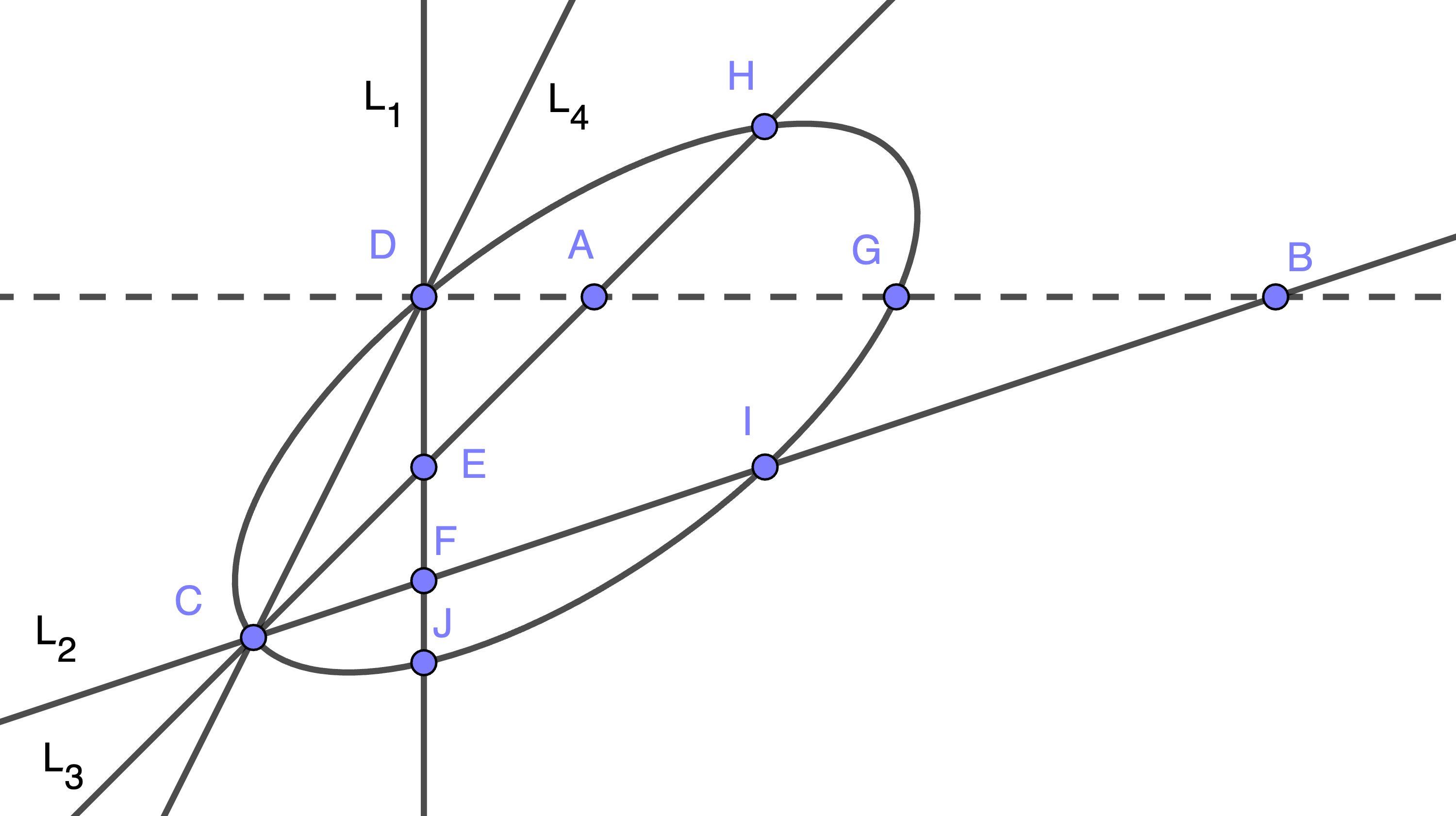
Figure 1. Curve configuration for Construction 5.1

Construction 5.1.

Let $L_{4}$ be a line in $\mathbb{P}^{2}$, $D$ the point of intersection with $\mathbb{P}^{1}_{\infty}$ and $C$ an other point on $L_{4}$. Now choose $L_{1}$ and $L_{2}$ through $C$ and $L_{3}$ through $D$. Finally choose a conic $Q$ through $C$ and $D$. This gives a $2+0+1+1+1+1+3=9$ dimensional family of curve configurations. The union $U$ of all these curves has degree $6$. Outside of $C$ and $D$ it has $5$ more nodes labeled $E,F,H,I,J$ in Figure 1.

The degree $t$ of $X=V(U,U_{x},U_{y})$ at the special points is:

point	t
$4$-fold point at $C$	9
$3$-fold point at $D$	6
nodes at $E,F,H,I,J$	5

Therefore the expected number of degree $3$syzygies is

$$\eta =2{d+2\choose 2}+{d+1\choose 2}-{d+e+1\choose 2}+\deg X$$

$$\geq 2\cdot 10+6-45+20=1$$

Let $\omega$ be a differential form constructed from such a syzygy. Consider now the reducible curve $\Gamma=L_{1}\cup L_{2}\cup L_{3}\cup Q$. By Lemma 2.4 it is also an integral curve of $\omega$. Let $K_{L_{4}}$ and $K_{\Gamma}$ be the cofactor of the respective curves. Evaluating a the $4$-fold point $C$ and the nodes, we obtain the following expected matrix of values for $(K_{L_{4}}:K_{\Gamma}:d\omega)$:

$$\begin{pmatrix}0&1&1\\ 1&3&2\\ \end{pmatrix}\begin{tabular}[]{c}(at nodes)\\ (at $C$)\\ \end{tabular}$$

of which some rows might possibly be replaced by zeros.

The kernel of this matrix contains $(1,-1,1)^{t}$, so

$$K_{L_{4}}-K_{\Gamma}+d\omega$$

vanishes on $C,E,F,H,I,J$. If these points are in general position with respect to conics this implies that even

$$K_{L_{4}}-K_{\Gamma}+d\omega=0$$

as polynomials. By Darboux’ Theorem this shows then, that $\omega$ has a rational integrating factor.

It is now easy to check that

$$\omega= (-40x^{2}y-36xy^{2}-4y^{3}-80x^{2}-102xy-34y^{2}-60x-72y-40)dx$$

$$+(24x^{3}+16x^{2}y+2x^{2}+12xy-9x+2y-2)dy$$

has integral curves

$$L_{1} =y+2$$

$$L_{2} =4x+y+4$$

$$L_{3} =4x+1$$

$$L_{4} =2x+1$$

$$Q =2x^{2}+2xy+x+2y+2$$

in the above configuration, that $X$ has the expected degree, that the Darboux matrix has the expected number of syzygies, that $h^{1}({\mathcal{I}}_{X}(8))=0$ and that the points $C,E,F,H,I,J$ do not lie on a conic. Furthermore one checks that $\omega$ has only finitely many integral conics. (see our script example_9_6.m2 at [vBK24].

It follows that there exist a family $9$ dimensional family of degree $3$ differential forms with a rational integrating factor. Over a finite field one can also check, that the tangent space to the center variety at this point is at most $9$ dimensional by calculating the derivatives of the first $10$ focal polynomials in $\omega$. This proves that the constructed family is a component of the center variety.

Differential forms constructed in this way lie in the ideal $9.6$ found experimentally by Johannes Steiner [Ste11].

It seems to us, that this component is new.

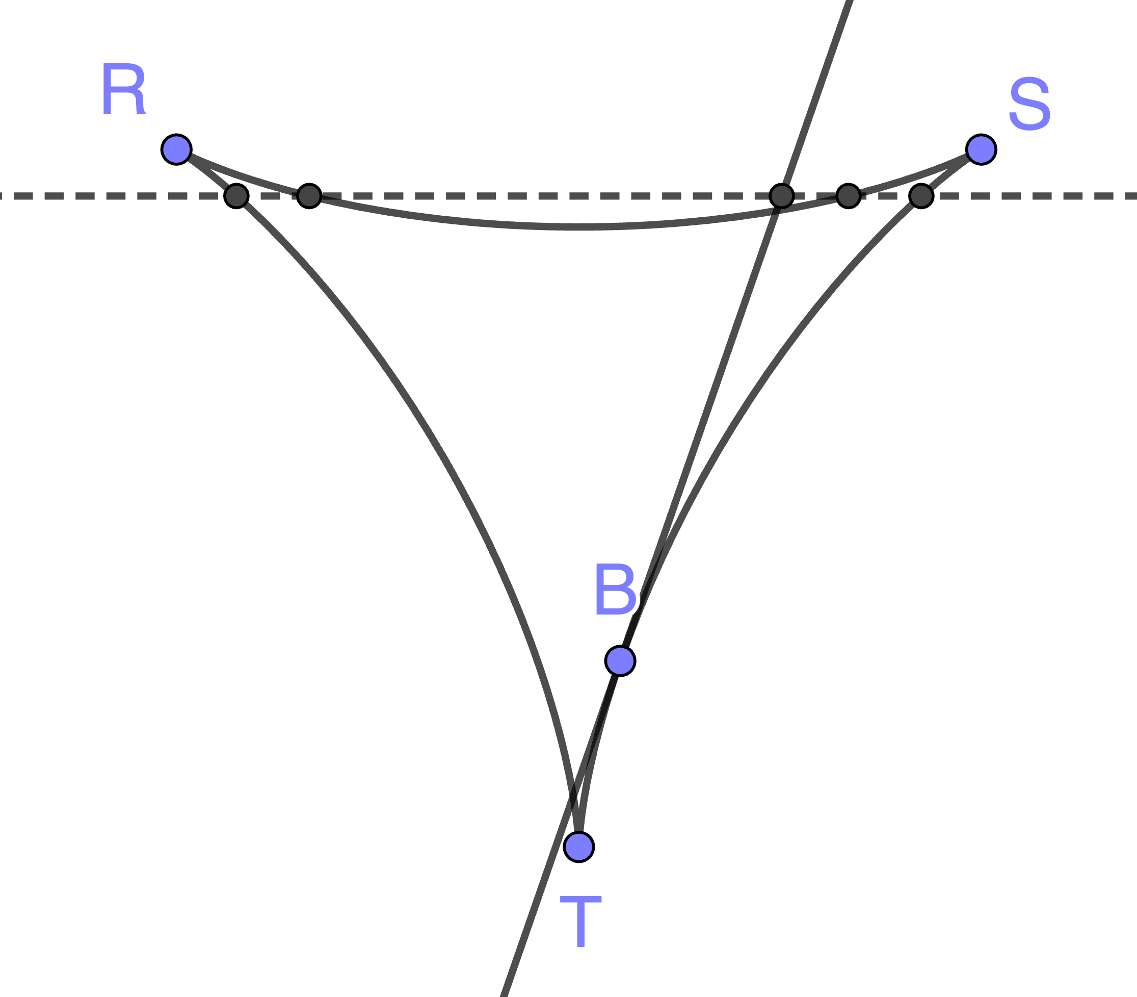
Figure 2. Curve configuration for Construction 5.2

Construction 5.2.

Let $C$ be a $3$-cuspidal curve with nodes labeled $R,S,T$ and a line $L$ tangent to $C$ in a point $B$ as considered in Examples 4.4 and 4.8 and Figure 2. By the following dimension count we have at least a $9$ dimensional family of such configurations.

plane quartic	14
3 cusps	-6
point B	1
tangent to B	0
sum	9

Let now $U=C\cup L$ be the union of the curves. The degree of $X$ defined by $(U,U_{x},U_{y})$ is at least $6+3+2=11$ since we have three cusps of $C$, a tacnode at $B$ and two nodes at the other intersection points.

The expected number of degree $3$ syzygies is therefore at least

$$\eta\geq 26-{3+5+1\choose 2}+11=1$$

Let now $\omega$ be a differential form constructed from such a syzygy and $K_{C},K_{L}$ the corresponding cofactors. We can predict the values of $(K_{L}:K_{C}:d\omega)$ at the special points by Proposition 4.1. Since we have $5$ points on $\mathbb{P}^{1}_{\infty}$ we can also apply Proposition 4.7 for general points on $\mathbb{P}^{1}_{\infty}$:

$$\begin{pmatrix}0&6&{5}\\ 2&2&{3}\\ 1&4&{4}\\ \end{pmatrix}\begin{tabular}[]{c}(at cusps)\\ (at $B$)\\ (at infinity)\\ \end{tabular}$$

where some lines might be replaced by zeros. Since $(4,5,-6)^{t}$ is in the kernel of this matrix

$$4K_{L}+5K_{C}-6d\omega$$

vanishes on $\mathbb{P}^{1}_{\infty}$ and at the points $R,S,T,B$. If the points $R,S,T,B$ do not lie on a line, this shows that

$$4K_{L}+5K_{C}-6d\omega=0$$

as polynomials and $\omega$ has a rational Darboux integrating factor. The necessary genericity conditions can be checked for example for

$$\omega= (-11x^{2}y+3xy^{2}+y^{3}-2x^{2}+xy+5y^{2}-2x+4y)dx$$

$$+(11x^{3}-3x^{2}y-xy^{2}+10x^{2}-4xy-y^{2}-x-y)dy$$

with integral curves

$$L =-7x+2y+1$$

$$C =x^{2}y^{2}-2x^{2}yw-2xy^{2}w+x^{2}w^{2}-2xyw^{2}+y^{2}w^{2}$$

where $w=x+y+1$. This proves that this construction describes $9$-dimensional component of degree $3$ differential forms with a center. Differential forms constructed in this way lie in Johannes Steiner’s experimental ideal 9.8.

Experimentally we also see that differential forms as constructed above automatically contain a further integral curves of degree $2$ and $3$ as well as infinitely many integral curves of degree $6$.

It seems to us, that this component is new.

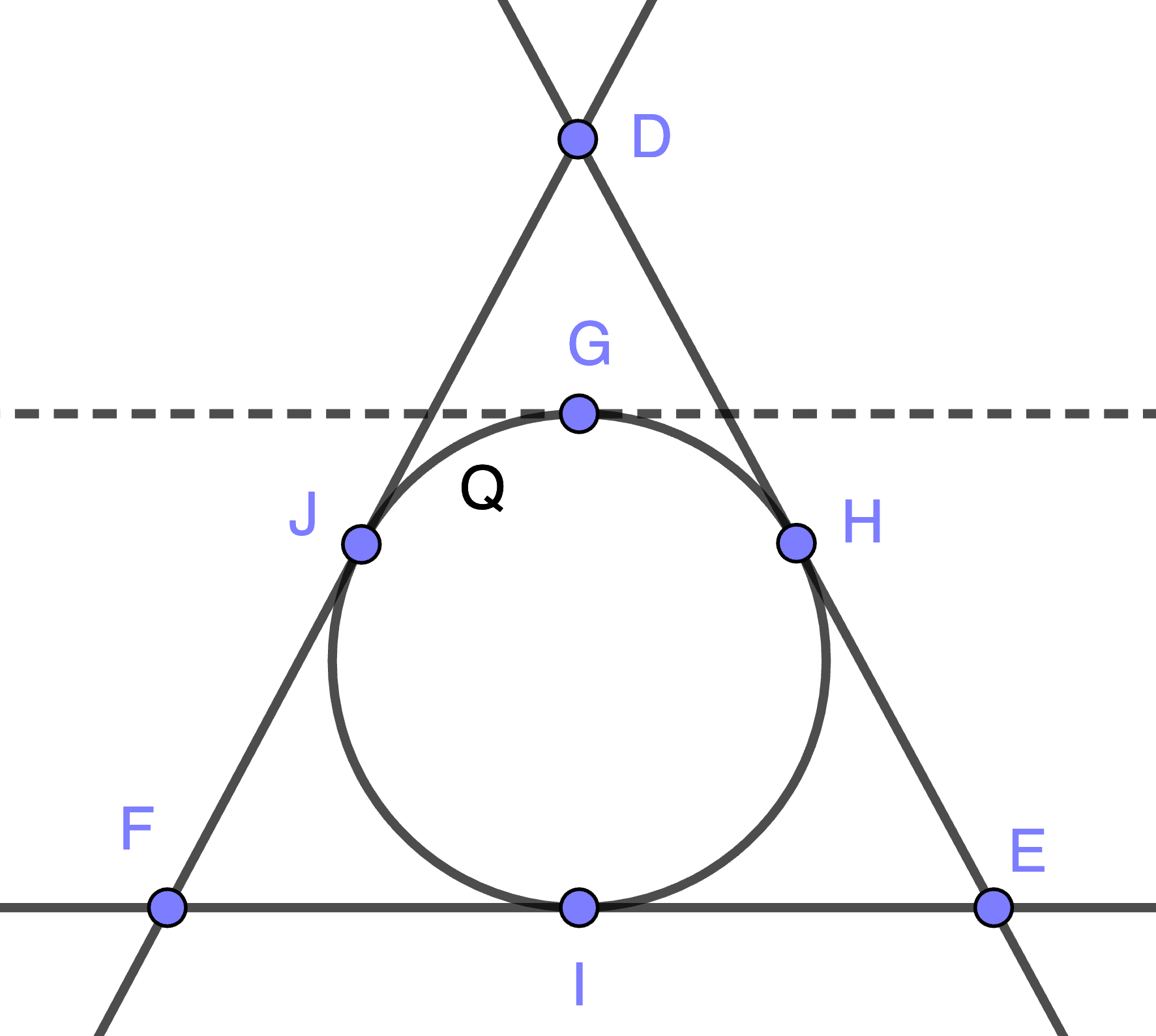
Figure 3. Curve configuration for Construction 5.3

Construction 5.3.

Choose a point $G$ on $\mathbb{P}^{1}_{\infty}$ and $3$ general points $H,I,J$ in the affine plane. Let $Q$ be a conic tangent at $G$ to infinity an passing through $H,I,J$. Let $T_{H}$, $T_{I}$ and $T_{J}$ the tangent lines to $G$ in the respective points and $D,E,F$ the intersection points of the tangent lines as shown in Figure 3. By the following dimension count we have a $7$ dimensional family of such configurations

point G	1
points H,I,J	6
quadric Q	0
sum	7

Let now $U=T_{H}\cup T_{I}\cup T_{J}\cup Q$. The degree of $X=V(U,U_{x},U_{y})$ at the special points is:

point	t
tangent to $\mathbb{P}^{1}_{\infty}$ at $C$	1
tacnodes at $H$,$I$,$J$	9
nodes at $E,F,G$	3

Therefore the expected number of degree $3$syzygies is

$$\eta =26-{3+5+1\choose 2}+13=3$$

Let $\omega$ be a differential form constructed from such a syzygy. Consider the triangle $T=T_{H}\cup T_{I}\cup T_{J}$, the inscribed conic $Q$ and their cofactors $K_{Q}$ and $K_{T}$. Evaluating at the special points we obtain:

$$\begin{pmatrix}0&1&{1}\\ 2&2&{3}\\ \end{pmatrix}\begin{tabular}[]{c}(at nodes)\\ (at tangent points)\\ \end{tabular}$$

where some rows might be replaced by zeros. Since $(1,2,-2)^{t}$ is in the kernel of this matrix

$$K_{Q}+2K_{T}-2d\omega$$

vanishes at the tangent points and the nodes. If these $6$ points do not lie on a conic, this shows that

$$K_{Q}+2K_{T}-2d\omega=0$$

as polynomials and $\omega$ has a rational Darboux integrating factor. The necessary genericity conditions can be checked for example with

$$\omega= (-2xy^{2}-2y^{3}+2xy+2y)dx$$

$$+(4x^{3}+2x^{2}y+xy^{2}-4xy-y^{2}-x-y)dy$$

Since we have a $7$ dimensional family of configurations and at $3$ syzygies of each, this proves that this construction describes $7+2=9$-dimensional component of degree $3$ differential forms with a center. Differential forms constructed in this way lie in Johannes Steiner’s ideal 9.9. It seems to us that this component is also new.

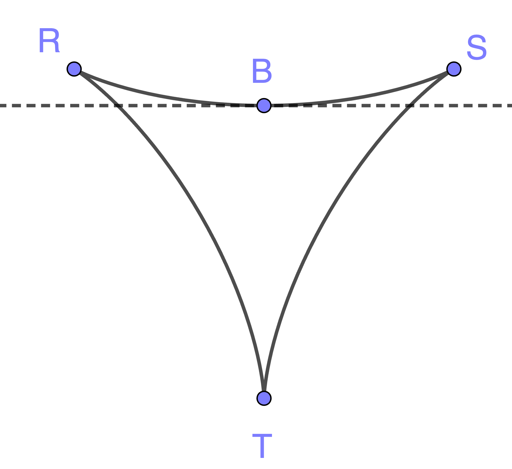
Figure 4. Curve configuration for Construction 5.4

Construction 5.4.

Consider a $3$ cuspidal quartic tangent to $\mathbb{P}^{1}_{\infty}$. Label the cusps with $R,S,T$ and the tangent point with $B$ as in Figure 4. There is a $14-3\cdot 2-1=7$ dimensional family of such configurations. The degree of $X$ defined by $(C,C_{x},C_{y})$ at the special points is

point	t
3 cusps	6
at $B$	1

Therefore the expected number of degree $2$ (!) syzygies is

$$\eta =6+6+3-{2+4+1\choose 2}+7=1$$

Let now $\omega$ be a differential form constructed from such a syzygy and let $K$ be the cofactor of $C$. Evaluating $K:d\omega$ at the cusps gives $(6:5)$. And therefore $5K-6d\omega$ vanishes there. Now $K$ and $d\omega$ are linear forms and therefore $5K-6d\omega=0$ as polynomials if the cusps do not lie on a line. In this case $\omega$ has a rational Darboux integrating factor $\mu$.

This component is not new. Differential forms of this family automatically have further integral curves of degree $2$ and $3$ in special position and coincide with the well known component of codimension $3$ of degree $2$ differential forms. At most our technique gives a new proof of Darboux integrability for differential forms of this type.

Now consider a general linear form $L$ and the differential form $L\omega$. It will be of degree $3$ and has an integrating factor $\frac{\mu}{L}$. Since one can check the necessary genericity conditions for

$$\omega=(x+1)\bigl{(} (-x^{2}+20xy+5y^{2}+x-5y)dx$$

$$+(-5x^{2}-20xy+y^{2}+5x-y)dy\bigr{)}$$

with integral curve

$$C =x^{2}y^{2}-2x^{2}yw-2xy^{2}w+x^{2}w^{2}-2xyw^{2}+y^{2}w^{2}$$

and $w=(1/8)(x+y-z)$, we have a $7$-dimensional family of configurations and a $3$ dimensional family of degree $3$ syzygies that give rise to an integrable degree $3$ differential forms. This gives again a $7+2=9$ dimensional component of the center variety.

Differential forms constructed in this way lie in Johannes Steiners’s ideal 9.10.

This component does not appear on Żoła̧dek’s lists, but possibly it was left out because the construction is a trivial extension of a well known degree $2$ component.

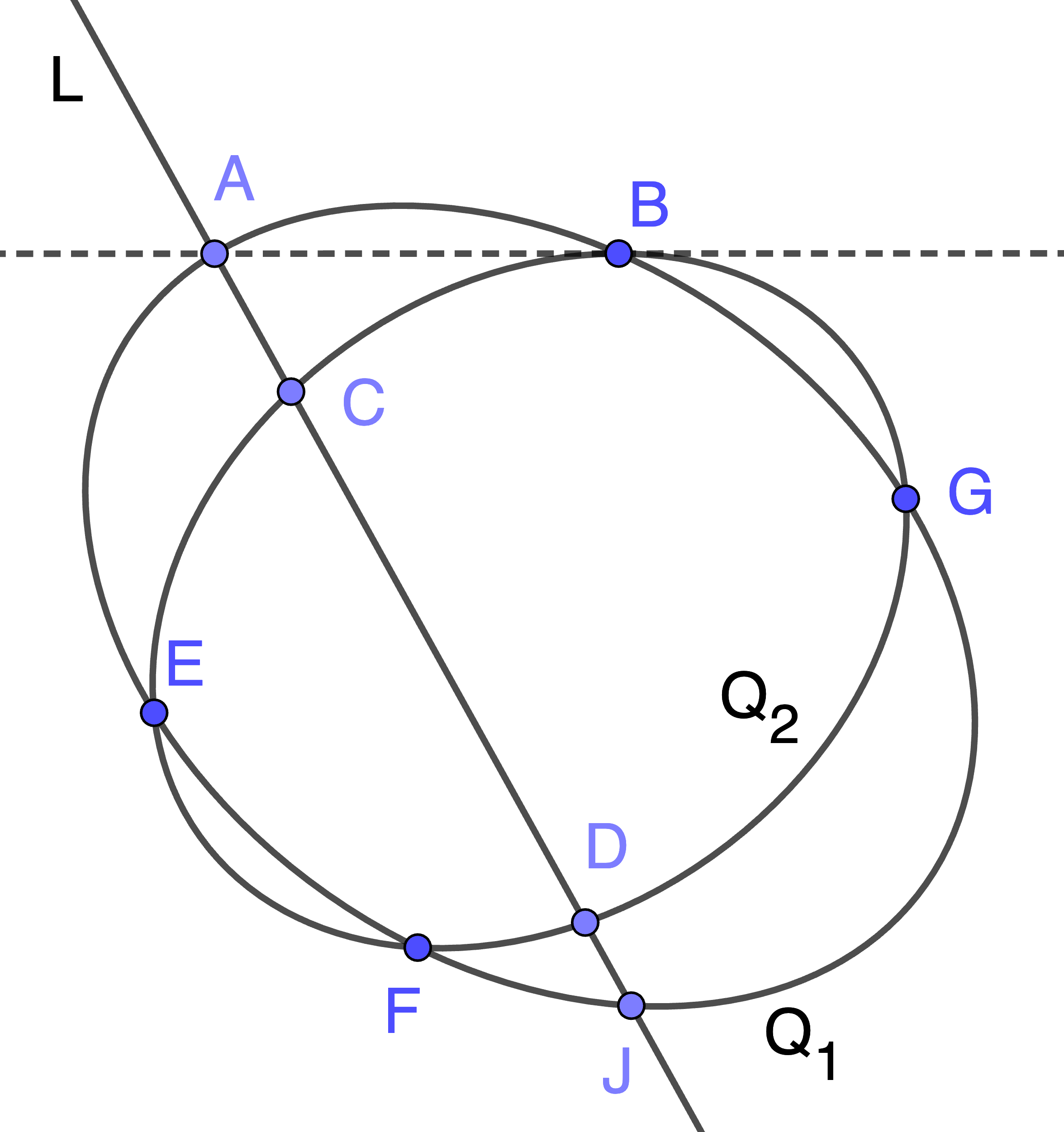
Figure 5. Curve configuration for Construction 5.5

Construction 5.5.

Consider a conic $Q_{1}$ that intersects $\mathbb{P}^{1}_{\infty}$ in points $A$ and $B$. Choose a second conic $Q_{2}$ tangent to $\mathbb{P}^{1}_{\infty}$ at $B$. Finally choos a line $L$ through $A$ as in Figure 5. By the following dimension count we have at least a $9$ dimensional family of such configurations.

conic $Q_{1}$	5
conic $Q_{2}$	3
line L	1
sum	9

Let now $U=Q_{1}\cup Q_{2}\cup L$ be the union of all curves. The degree of $X$ defined by $(U,U_{x},U_{y})$ at the special points is

point	t
$2$-fold point at $A$	$2$
$2$-fold point with tangent at $B$	$\geq 3$
$6$ nodes	$6$

The expected number of degree $3$ syzygies is therefore at least

$$\eta\geq 26-{3+5+1\choose 2}+11=1.$$

Let now $\omega$ be a differential form constructed from such a syzygy and $K_{U}$ the cofactor. The value of $(K_{U}:d\omega)$ at the $6$ nodes is $(1:1)$ and therefore $K_{U}-d\omega$ vanishes at all nodes. If the nodes do not lie on a conic this shows $K_{U}=d\omega$ and $\omega$ has a rational Darboux integrating factor.

The necessary genericity assumptions are satisfied by

$$\omega= (-68x^{3}-168x^{2}y-216xy^{2}-64y^{3}-41x^{2}-98xy-16y^{2}+57x+46y)dx$$

$$+(-52x^{3}+32x^{2}y+32xy^{2}+20x^{2}+24xy+80x+24y)dy$$

with integral curves

$$L =x+2y$$

$$Q_{1} =2x^{2}+4xy+x+1$$

$$Q_{2} =15x^{2}-19x-4y.$$

We obtain a $9$-dimensional component of the center variety in degree $3$. This component is not completely new: it contains Żoła̧dek’s family $CD_{28}$ as a subset of codimension $1$. Its differential forms lie in Johannes Steiner’s ideal 9.14.

Experimentally differential forms of this construction automatically have another algebraic integral curve of degree $3$ and infinitely many algebraic integral curves of degree $4$.

Table 1 gives an overview of the current situation in codimension $9$ according to our knowledge.

Steiner’s experimental ideals	Żoła̧dek’s families	this paper
9.1	$CR_{9}$
9.2	$CD_{8}$
9.3
9.4	$CR_{15}$
9.5	$CD_{21}$, $CR_{10}$
9.6		Construction 5.1
9.7
9.8		Construction 5.2
9.9		Construction 5.3
9.10		Construction 5.4
9.11	$(CD_{30})$
9.12
9.13
9.14	$(CD_{28})$	Construction 5.5

Table 1. Overview of codimension $9$ components. Numbers in brackets denote families that lie in the given component, but do not fill up the whole component.

References

- [Chr05] Colin J. Christopher. Centre conditions for a class of polynomial differential systems. preprint, 2005.
- [CLPW12] Colin Christopher, Jaume Llibre, Chara Pantazi, and Sebastian Walcher. Inverse problems in Darboux’ theory of integrability. Acta Appl. Math., 120:101–126, 2012.
- [CRŻ97] L. A. Cherkas, V. G. Romanovskii, and H. Żoła̧dek. The centre conditions for a certain cubic system. Differential Equations Dynam. Systems, 5(3-4):299–302, 1997. Planar nonlinear dynamical systems (Delft, 1995).
- [Dar78] G. Darboux. Mémoire sur les équations différentielles algébriques du permier ordre et du premier degré (Mélanges). Bull. Sci. Math., 2:60–96;123–144; 151–200, 1878.
- [Dul08] M. H. Dulac. Determination et integration d’une certaine classe d’equations differentielles ayant pour point singulier un centre. Bull. Sci. Math., 32:230–252, 1908.
- [Fro34] M. Frommer. Über das Auftreten von Wirbeln und Strudeln (geschlossener und spiraliger Integralkurven) in der Umgebung rationaler Unbestimmtheitsstellen. Math. Ann., 109:395–424, 1934.
- [GLS07] G.-M. Greuel, C. Lossen, and E. Shustin. Introduction to singularities and deformations. Springer Monographs in Mathematics. Springer, Berlin, 2007.
- [GS] Daniel R. Grayson and Michael E. Stillman. Macaulay2, a software system for research in algebraic geometry. Available at http://www.math.uiuc.edu/Macaulay2.
- [Poi85] H. Poincaré. Sur les courbes définies par les équations différentielles. Journal de Mathématiques Pures et Appliquées, 4e série, 1:167–244, 1885.
- [Ste11] Johannes Steiner. Untersuchung der Komponenten der Zentrumsvarietät durch Interpolation. Bachelor Thesis, Georg-August-Universität Göttingen, January 2011.
- [vBK10] Hans-Christian Graf v. Bothmer and Jakob Kröker. A survey of the Poincaré center problem in degree 3 using finite field heuristics, 2010.
- [vBK24] Hans-Christian Graf v. Bothmer and Jakob Kröker. centerfocus: Macaulay2 packages for studying the poincaré center problem. https://github.com/bothmer/centerfocus, 2024.
- [vW05] Wolf v. Wahl. personal communication, 2005.
- [Żoł94] Henryk Żoła̧dek. The classification of reversible cubic systems with center. Topol. Methods Nonlinear Anal., 4(1):79–136, 1994.
- [Żoł96] Henryk Żoła̧dek. Remarks on: “The classification of reversible cubic systems with center” [Topol. Methods Nonlinear Anal. 4 (1994), no. 1, 79–136; MR1321810 (96m:34057)]. Topol. Methods Nonlinear Anal., 8(2):335–342 (1997), 1996.