Graphons of Line Graphs

Abstract

We consider the problem of estimating graph limits, known as graphons, from observations of sequences of sparse finite graphs. In this paper we show a simple method that can shed light on a subset of sparse graphs. The method involves mapping the original graphs to their line graphs. We show that graphs satisfying a particular property, which we call the square-degree property are sparse, but give rise to dense line graphs. This enables the use of results on graph limits of dense graphs to derive convergence. In particular, star graphs satisfy the square-degree property resulting in dense line graphs and non-zero graphons of line graphs. We demonstrate empirically that we can distinguish different numbers of stars (which are sparse) by the graphons of their corresponding line graphs. Whereas in the original graphs, the different number of stars all converge to the zero graphon due to sparsity. Similarly, superlinear preferential attachment graphs give rise to dense line graphs almost surely. In contrast, dense graphs, including Erdős–Rényi graphs make the line graphs sparse, resulting in the zero graphon.

1 Introduction

A graphon is the limit of a converging graph sequence. Graphons of dense graphs are useful as they can act as a blueprint and generate graphs of arbitrary size with similar properties. But for sparse graphs this is not the case. Sparse graphs converge to the zero graphon, making the generated graphs empty or edgeless. Thus, the classical graphon definition fails for sparse graphs. Several methods have been proposed to overcome this limitation and to understand sparse graphs more deeply. However, the fragile nature of sparse graphs makes these methods mathematically complex. Graphons are useful in machine learning as a prior distribution on graphs. Graphons provide an interesting connection between combinatorial, probabilistic, and analytical problems, leading to many new approaches for graph modelling.

The obvious use of graphons is to predict a network and its properties at a future time point when the network is large (Chayes, 2016). The fact that graphons are compact objects with the ability to generate arbitrarily large networks is an attractive feature. It is also studied in the context of exchangeable arrays (Orbanz & Roy, 2015). In addition to network prediction, graphons are used in a myriad ways including in tranfer learning neural networks (Ruiz et al., 2020), graph embeddings (Davison & Austern, 2023) and motif sampling (Lyu et al., 2023). They are also of interest to problems in extremal graph theory, the study of large graphs and random matrix theory. Graphons have had wide application in statistical physics and network theory.

The theory of graphons of dense graphs is well developed, and is based on the Aldous-Hoover theorem. For a graphon to exist the sequence of graphs need to converge in homomorphism density, which can be thought of as subgraph density. However, a limitation of such graphons is that they produce dense graphs when the graphon is non-zero. If the graphon is zero everywhere, then it is of little use as it can only produce an empty graph. Thus, sparse graphs cannot be modelled using this approach. There are results for graphons of sparse graphs, as the classical constructions prevent models where the number of edges grow sub-quadratically with respect to the number of nodes. Previous approaches for sparse graphons include constructions using Kallenberg exchangeability (Caron & Fox, 2017), stretched graphons (Borgs et al., 2018) and graphexes (Borgs et al., 2021).

In this paper, we propose a new way to model sparse graphons by modeling the graphon of the corresponding line graph. Line graphs map edges to vertices and connects edges when edges in the original graph share a vertex. For a graph $G_{n}$ with $n$ nodes, a line graph $H_{m}:=L(G_{n})$ is a graph where each of the $m$ edges of the original graph $G_{n}$ is a node of $H_{m}$. Many properties of the original graph $G_{n}$ have a corresponding property in the line graph $H_{m}$. In contrast to previous approaches to graphons of sparse graphs that required complex mathematical machinery, our approach builds on the results of graphons on dense graphs directly. We discover that if graphs $G_{n}$ have the property that the sum of the squares of the node degrees is greater than the square of the number of edges, then the corresponding line graphs $H_{m}$ are dense. This relationship between $G_{n}$ and $H_{m}$ may be of independent interest. We show that sparse graphs $G_{n}$ that satisfy the so called “square-degree property” have line graphs $H_{m}$ that result in non-zero graphons.

We provide some background in Section 2, and present our discovery connecting graphs $G_{n}$ with their line graphs $H_{m}$ in Section 3. We show that graphs $G_{n}$ that satisfy the square-degree property have convergent edge densities and homomorphism densities. We derive the graphons for disjoint star graphs in Section 4 and illustrate the empirical behaviour of estimation on sparse graphs in Section 4.4. We derive graphons of line graphs for preferential attachment and Erdos-Renyi graphs in Section 5.

Contributions of this paper

• We propose a property of sparse graphs, the square-degree property (Definition 3.3) which allows us to find sparse graphs whose line graphs are dense. In particular, sparse graphs with square-degree property have dense line graphs, and under certain conditions have line graph limits (Section 3.4).

• We prove that for disjoint star graphs, the corresponding line graphs are dense and hence have graph limits (Section 4). Furthermore, we show that certain preferential attachment graphs have dense line graphs that converge to non-zero graphons under certain conditions (Section 5.1).

• We illustrate with empirical graphons the utility of line graphs for sparse graphs in Section 4.4.

2 Notation and Preliminaries

A simple graph is a graph without loops or multiple edges between the same nodes. We only consider simple graphs and sequences of simple graphs in this paper.

2.1 Line graphs

Let $G$ denote a graph. If $G$ has at least one edge, then its line graph is the graph whose vertices are the edges of $G$, with two of these vertices being adjacent if the corresponding edges are adjacent in $G$ (Beineke & Bagga, 2021). Figure 1 shows an example of a graph and its line graph. The edges in the graph on the left are mapped to the vertices in the line graph (on the right) as can be seen from the numbers.

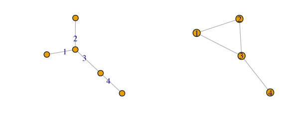
Figure 1: A graph on the left and its line graph on the right.

We denote the line graph operation by $L$, i.e., for a graph $G$ we denote its line graph by $H:=L(G)$. In terms of notation we make a distinction between graphs $G$ and line graphs $H$, i.e., we use the letter $H$, with and without subscripts, to denote line graphs.

Rather than a single graph $G$, we are interested in graph sequences. The exact type of sequences which forms our interest will be made clear by the end of this section. Let $\{G_{n}\}_{n=1}^{\infty}$ denote a graph sequence. The index $n$ denotes the number of nodes in $G_{n}$ and let the number of edges be given by $m$. We denote the line graph of $G_{n}$ by $H_{m}:=L(G_{n})$ as $H_{m}$ has $m$ nodes.

We use standard graph theory notation to denote specific types of graphs. As customary $K_{n}$ denotes a complete graph of $n$ nodes, and $K_{s,r}$ denotes a complete bi-partite graph of partition sizes $s$ and $r$, i.e., there are $s$ nodes in one subset completely connected to $r$ nodes in the other subset. When $s=1$ we get star graphs; $K_{1,n}$ denotes a star with $n+1$ vertices, where $n$ vertices are connected to the hub vertex.

Definition 2.1.

If $G$ is a graph whose line graph is $H$, that is, $L(G)=H$, then $G$ is called the root of $H$.

Whitney (1932) showed that the structure of a graph can be recovered from its line graph with one exception: if the line graph $H$ is $K_{3}$, a triangle, then the root of $H$ can be either $K_{1,3}$, a star or $K_{3}$ a triangle. This follows from the following theorem as stated in Harary (1969):

Theorem 2.2 (Whitney1932, Harary 1969).

Let $G$ and $G^{\prime}$ be connected graphs with isomorphic line graphs. Then $G$ and $G^{\prime}$ are isomorphic unless one is $K_{3}$ and the other is $K_{1,3}$.

By simply creating edges corresponding to vertices in line graph $H$ and connecting them by merging the vertices if there is an edge between the vertices in $H$ we can obtain the the graph $G$, such that $H=L(G)$. Thus, if $H$ is a line graph and it is not $K_{3}$, then we can talk about $L^{-1}(H)$.

We state some preliminary results on line graphs covered in Chapter 1 of Beineke & Bagga (2021).

Lemma 2.3.

Let $G$ be a non-null graph with $n$ vertices and $m$ edges. Let $H=L(G)$. Then

1. $H$ has $m$ vertices and $\frac{1}{2}\sum(\text{deg }\,v)^{2}-m$ edges

2. If $G$ is an $r$-regular graph then $H$ is $2(r-1)$-regular and has $\frac{nr}{2}$ vertices.

3. If $G$ is a path $P_{n}$, then $H$ is also a path of $n-1$ vertices, i.e., $H=P_{n-1}$.

4. If $G$ is a non-trivial connected graph, then $H$ is also connected.

5. If $G$ is a cycle $C_{n}$ of $n$ vertices, then $H$ is also a cycle $C_{n}$ of $n$ vertices.

6. If $G$ is a star, i.e., $G=K_{1,n-1}$, then $H$ is a complete graph of $n-1$ vertices, i.e. $H=K_{n-1}$.

The edge density of a graph $G$ with $n$ nodes and $m$ edges is given by $\text{density}(G)=\frac{2m}{n(n-1)}$. Thus, from Lemma 2.3(1) the edge density of $H=L(G)$ is given by

$$\text{density}(H)=\frac{\frac{1}{2}\sum(\text{deg }\,v^{2})-m}{\frac{1}{2}m(m-1)}\,,$$ (1)

where $\text{deg }v$ denotes the degree distribution of graph $G$ and $\text{deg }v^{2}$ denotes the vector of squared degrees in $G$. We refer to the edge density simply as density.

2.2 Graphons

Next we turn our attention to graphons. A graphon is a symmetric, measurable function $W:[0,1]^{2}\rightarrow[0,1]$ often used to describe both the limiting properties of graph sequences as well as the graph generation process (Borgs et al., 2011). We define some terms often used in the graphon literature.

Definition 2.4.

A graph homomorphism from $F$ to $G$ is a map $f:V(F)\to V(G)$ such that if $uv\in E(F)$ then $f(u)f(v)\in E(G)$. (Maps edges to edges.) Let $\text{Hom}(F,G)$ be the set of all such homomorphisms and let $\hom(F,G)=|\text{Hom}(F,G)|$. Then homomorphism density is defined as

$$t(F,G)=\frac{\hom(F,G)}{|V(G)|^{|V(F)|}}\,.$$

The number of homomorphisms $\hom(F,G)$ is given by

$$\hom(F,G)=\sum_{\phi:V(F)\to V(G)}\prod_{uv\in E(F)}\beta_{\phi(u)\phi(v)}(G)$$

where $\beta_{ij}(G)$ is the weight of edge $ij$ in graph $G$, which equals either 1 or 0 in unweighted graphs. For a graphon $W$, the homomorphism density is defined as

$$t(F,W)=\int_{[0,1]^{|V(F)|}}\prod_{ij\in E(F)}W(x_{i},x_{j})\,dx\,.$$

A graph homomorphism is an edge preserving map from one graph to another. The homomorphism density is useful as it is bounded even when the number of homomorphisms $\hom(F,G)$ go to infinity.

Definition 2.5.

The cut norm of graphon $W$ (Frieze & Kannan, 1999; Borgs et al., 2008) is defined as

$$\lVert W\rVert_{\square}=\sup_{S,T}\left|\int_{S\times T}W(x,y)\,dxdy\right|\,,$$

where the supremum is taken over all measurable sets $S$ and $T$ of $[0,1]$.

Definition 2.6.

Given two graphons $W_{1}$ and $W_{2}$ the cut metric (Borgs et al., 2008) is defined as

$$\delta_{\square}(W_{1},W_{2})=\inf_{\varphi}\left\lVert W_{1}-W_{2}^{\varphi}\right\rVert_{\square}\,,$$

where the infimum is taken over all measure preserving bijections $\varphi:[0,1]\rightarrow[0,1]$.

Let $\mathcal{W}$ denote the space of graphons, i.e., $\mathcal{W}=\{W\in\mathcal{W}\}$. Then, the cut metric is a pseudo-metric in $\mathcal{W}$ because $\delta_{\square}(W_{1},W_{2})=0$ does not imply $W_{1}=W_{2}$, i.e., $\delta_{\square}(W_{1},W_{2})\geq 0$ for $W_{1}\neq W_{2}$. However the cut metric $\delta_{\square}$ is a metric on the quotient space $\tilde{\mathcal{W}}=\mathcal{W}/\sim$ where $f\sim g$ if $f(x,y)=g(\sigma x,\sigma y)$ for some measure preserving $\sigma$.

Definition 2.7.

Uniformly pick $x_{1},x_{2},\ldots x_{n}$ from $[0,1]$. A W-random graph $\mathbb{G}(n,W)$ has the vertex set $1,2,\ldots n$ and vertices $i$ and $j$ are connected with probability $W(x_{i},x_{j})$.

We can think of $W$-random graphs as graphs sampled from the graphon $W$. We will use $W$-random graphs in our experiments.

The homomorphism density is used to define graph convergence.

Definition 2.8 ((Borgs et al., 2008)).

A graph sequence $\{G_{n}\}_{n}$ is said to be convergent if $t(F,G_{n})$ converges as $n$ goes to infinity for any simple graph $F$.

Every finite, simple graph $G$ can be represented by a graphon $W_{G}$, which we call its empirical graphon.

Definition 2.9.

Given a graph $G$ with $n$ vertices labeled $\{1,\ldots,n\}$, we define its empirical graphon $W_{G}:[0,1]^{2}\rightarrow[0,1]$ as follows: We split the interval $[0,1]$ into $n$ equal intervals $\{I_{1},I_{2},\ldots,I_{n}\}$ (first one closed, all others half open) and for $x\in I_{i},y\in I_{j}$ define

$$W_{G}(x,y)=\begin{cases}1&\,\text{if}\quad ij\in E(G)\\ 0&\,\text{otherwise}\,,\end{cases}$$

where $E(G)$ denotes the edges of $G$. The empirical graphon replaces the the adjacency matrix with a unit square and the $(i,j)$th entry of the adjacency matrix is replaced with a square of size $(1/n)\times(1/n)$.

The cut metric between graphs $G$ and $G^{\prime}$ is defined as $\delta_{\square}\left(G,G^{\prime}\right)=\delta_{\square}\left(W_{G},W_{G^{\prime}}\right)$. The cut metric between a graph $G$ and a graphon $U$ is defined as $\delta_{\square}\left(G,U\right)=\delta_{\square}\left(W_{G},U\right)$.

Borgs et al. (2008) prove the following theorem for convergent graph sequences.

Theorem 2.10 (Borgs et al. (2008)).

For every convergent sequence $\{G_{n}\}_{n}$ of simple graphs there is a graphon $W$ with values in $[0,1]$ such that $t(F,G_{n})\rightarrow t(F,W)$ for every simple graph $F$. Moreover for every graphon $W$ with values in $[0,1]$ there is a convergent sequence of graphs satisfying this relation.

Theorem 2.11 (Borgs et al. (2011)).

A sequence of graphs $\{G_{n}\}_{n}$ is convergent if and only if it is Cauchy in the $\delta_{\square}$ distance. The sequence $\{G_{n}\}_{n}$ converges to $W$ if and only if $\delta_{\square}(W_{G_{n}},W)\to 0$. Furthermore, if this is the case, and $|V(G_{n})|\to\infty$, then there is a way to label the nodes of the graphs $G_{n}$ such that $\lVert W_{G_{n}}-W\rVert_{\square}\to 0$.

2.2.1 Line graphs and edge exchangeability

As discussed above edge-exchangeable graphs can exhibit sparsity (Janson, 2018). Here we show the link between line graphs and edge exchangeability.

Figure 2 shows the connection between vertex and edge exchangeability when we map from graphs to line graphs. Graph $G$ is shown on the top left and its line graph $H=L(G)$ is shown on the top right. The graph on the bottom right $H^{\prime}$ is $H$ with vertices permuted. Let us call the graph on the bottom left $G^{\prime}$. Following definition 2.1 we can see that $G^{\prime}$ is the root of $H^{\prime}$ , i.e., $H^{\prime}=L(G^{\prime})$. Furthermore, the vertex permutation $\phi$ relabeled the vertices $(1,2,3,4)$ in $H$ to $(2,3,4,1)$ in $H^{\prime}$. We see the same permutation occurs in edges from $G$ to $G^{\prime}$, i.e. $G^{\prime}$ is an edge permuted version of $G$. This is not surprising as line graphs map edges to vertices.

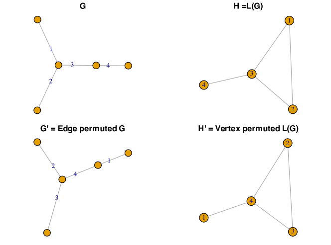
Figure 2: Vertex and edge exchangeability in graphs and line graphs. Graphs $G$ and $H=L(G)$ on the top row. Graph $H^{\prime}$ is a vertex permuted version of $H$. We see that $H^{\prime}=L(G^{\prime})$, where $G^{\prime}$ is the edge permuted version of $G$.

2.2.2 Edge vs homomorphism density

In this study we mention different types of convergence: convergence with respect to homomorphism density (Definition 2.4), cut metric (Definition 2.6), and edge density (Equation 1). Homomorphism density convergence is subgraph convergence. Suppose $\{G_{n}\}_{n}$ converges in homomorphism density, then for any graph $F$ the sequence $\{t(F,G_{n})\}_{n}$ converges. That is, the edge density, triangle density, 4-cycle density and all such densities converge. Convergence in homomorphism density is equivalent to convergence in the cut metric as shown by Borgs et al. (2011). In contrast, edge density convergence is the same as convergence of the single sequence $\{t(\leavevmode\hbox to10.46pt{\vbox to4pt{\text{[drawing]}}},G_{n})\}_{n}$. As edge density is given by $2|E(G_{n})|/n(n-1)$ and $t(\leavevmode\hbox to10.46pt{\vbox to4pt{\text{[drawing]}}},G_{n})=2|E(G_{n})|/n^{2}$ convergence in one implies convergence in the other. The denominators are different because the edge density excludes the diagonal of the adjacency matrix whereas $\{t(\leavevmode\hbox to10.46pt{\vbox to4pt{\text{[drawing]}}},G_{n})\}_{n}$ includes it (see Definition 2.4). However, edge density is much weaker and does not give us subgraph convergence.

We use edge density to characterize a bigger space of graph sequences – sequences that do not converge either in the cut metric or in edge density. The use of $\liminf$ in the definition of dense graph sequences (Definition 3.1) means that we do not need convergence of edge densities to call a graph sequence dense.

2.3 Related work

2.3.1 Graphons of sparse graphs

Caron & Fox (2017) set aside the discrete version of exchangeability and consider its continuous counterpart – Kallenberg exchangeability (Kallenberg, 1990). They consider exchangeable point processes and model graphs using completely random measures. They show that by selecting an appropriate Lévy measure, they can construct sparse or dense graphs. Collaborations led by Borgs and Chayes have resulted in considerable work on sparse graph limits. Borgs et al. (2017) consider sparse graph convergence by introducing a new notion of convergence called LD-convergence, which is based on the theory of large deviations. The large deviations rate function is considered to be the limit object for the sparse graph sequence. In Borgs et al. (2018), they introduce stretched graphons as a way to overcome the zero graphon, which is the natural limit of sparse graphs. They consider both the rescaled graphon introduced by Bollobás & Riordan (2011) and the stretched graphon as means of representing sparse graph limits. In Borgs, Chayes, Cohn & Zhao (2019) they develop the theory of $L^{p}$ graphons, which provides convergence for sparse graphs with the flexibility to account for power laws. Borgs, Chayes, Cohn & Veitch (2019) and Borgs et al. (2021) consider graphexes – a triple including a positive number, a positive integrable function and a graphon – as a framework for modelling sparse graphs.

Edge-exchangeability is another avenue used to model sparse graphs. Instead of considering exchangeability of vertices, edges are labelled and their permutations are considered. Crane & Dempsey (2018, 2019) introduce edge-exchangeable network models and show that these models allow for sparse structure and power-law degree distributions. Cai et al. (2016) consider projective, edge-exchangeable graphs and obtain sparsity results for all Poisson point process-based graph frequency models. Janson (2018) extends the model put forward by Crane & Dempsey (2018) and investigate different types of graphs that can be generated by this model. He shows that graphs ranging from dense to very sparse graphs can be generated by using the Poisson construction.

2.3.2 Other graphon applications

Possibly due to its rich mathematical context, graphons are used in many topics in machine learning. For example, it is desirable for a machine learning model to be transferable. Ruiz et al. (2020) propose graphon neural networks as the limit of graph neural networks (GNNs) with the aim of producing transferable GNNs. They show that GNNs are transferable between deterministic graphs obtained from the same graphon. Graphons and the associated theory is used to bolster theoretical aspects of other topics. Levie (2023) propose a graph signal similarity measure for message passing neural networks based on the graphon cut distance. Hence they extend the cut distance to graph signals. Graph embeddings are used for a myriad of downstream tasks such as node classification, clustering and link prediction. Davison & Austern (2023) investigate theoretical aspects of graph embeddings and show that embedding methods implicitly fit graphon models. Under the assumption the graph is exchangeable, they describe the limiting distribution of embeddings learned via subsampling the network. Graph homomorphisms are closely connected to graphons. Lyu et al. (2023) introduce motif sampling, which essentially sampling graph homomorphisms uniformly at random. They propose two MCMC algorithms for sampling random graph homomorphisms.

3 Sparse graphs with dense line graphs

In this section, we show that there are sparse graphs whose line graphs are dense. In particular we show in Theorem 3.6 that sparse graphs with square-degree property (Definition 3.3) have corresponding line graphs that are dense, and vice versa. We show in Section 3.4 that under certain conditions, the corresponding line graphs converge with respect to the homomorphism density, leading to graphons of line graphs. Therefore, this enables us to define a novel approach to defining graph limits for sparse graphs by their associated line graphs. Recall we denote graph sequences as $\{G_{n}\}_{n}$ and the corresponding line graph sequence as $\{H_{m}\}_{m}$. If the sequences converge, then we consistently use $W$ and $U$ for graphons corresponding to $\{G_{n}\}_{n}$ and $\{H_{m}\}_{m}$ respectively. We defer many of the proofs of lemmas and theorems to Appendix A.

3.1 Graph sequences

Definition 3.1 (Dense graph sequences).

A sequence of graphs $\{G_{n}\}_{n}$ is dense if the number of edges $m$ grow quadratically with the number of nodes $n$, i.e.,

$$\liminf_{n\to\infty}\frac{m}{n^{2}}=c>0\,.$$

We denote the set of all dense graph sequences by $D$.

Definition 3.2 (Sparse graph sequences).

A sequence of graphs $\{G_{n}\}_{n}$ is sparse if the number of edges $m$ grow sub-quadratically with the number of nodes $n$, i.e.,

$$\lim_{n\to\infty}\frac{m}{n^{2}}=0\,.$$

We denote the set of all sparse graph sequences by $S$.

For dense graph sequences, the density is bounded from below by a non-zero constant, whereas for sparse graph sequences it goes to zero. The density or $m/n^{2}$ of a sequence of dense graphs $\{G_{n}\}_{n}$ does not necessarily converge; the $\liminf$ is strictly positive, i.e., any converging subsequence has strictly positive density as $n\to\infty$. In contrast, the density or $m/n^{2}$ of sparse graphs converge to zero, i.e., the limit is equal to zero, not just the $\liminf$. The set of dense graph sequences $D$ and the set of sparse graph sequences $S$ is non-intersecting. Furthermore, the complement of the union of $D$ and $S$, $\overline{D\cup S}$ is non-empty. It contains graph sequences $\{G_{n}\}_{n}$ such that $\liminf_{n\to\infty}m/n^{2}=0\neq\limsup_{n\to\infty}m/n^{2}$, i.e, it is a mixture of dense and sparse graph sequences with the density of different subsequences converging to different limits with some converging to zero.

Next we define a property of a graph sequence that we call the square-degree property .

Definition 3.3 (Square-degree property $Sq$).

Let $\{G_{n}\}_{n}$ denote a sequence of graphs. We say that $\{G_{n}\}_{n}$ exhibits the square-degree property if there exists some $c_{1}>0$ and $N_{0}\in\mathbb{N}$ such that for all $n\geq N_{0}$ we have

$$\sum\text{deg }v_{i,n}^{2}\geq c_{1}\left(\sum\text{deg }v_{i,n}\right)^{2}\,.$$

We denote the set of graph sequences satisfying the square-degree property by $S_{q}$, i.e. if $\{G_{n}\}_{n}$ satisfies $Sq$ then $\{G_{n}\}_{n}\in S_{q}$.

We note that Cauchy-Schwarz inequality gives $c_{1}=1/n$, which is not satisfactory as we need a strictly positive lower bound $c_{1}>0$ for all $n$. The square-degree property says that the ratio between the sum of the degree squared and square of the sum of degrees is bounded from below as $n$ goes to infinity. As the degree of a node is either zero or positive, this cannot be satisfied if the degree distribution is uniform, because then the sum of the mixed product terms $\text{deg }v_{i,n}\times\text{deg }v_{j,n}$ would hold the bulk weight compared to the square terms $(\text{deg }v_{i,n})^{2}$, especially as there are $n\choose{2}$ mixed product terms and only $n$ square terms. Therefore, we expect a graph sequence satisfying this property to have some inequalities in the degree distribution. For example, it may contain a set of “big player” nodes with large degree values.

Using the square-degree property $Sq$ we characterize graph sequences $\{G_{n}\}_{n}$ as shown in Figure 3, in which the blue text represents results obtained in this paper. If a graph sequence converges in homomorphism density, then by Theorem 2.10 a graphon exists. In such instances, we consistently use $W$ and $U$ for graphons corresponding to $\{G_{n}\}_{n}$ and $\{H_{m}\}_{m}$ respectively. It is well-known that for converging dense graph sequences $\{G_{n}\}_{n}$, the graphon $W\neq 0$, while sparse graph sequences correspond to $W=0$. This can be easily verified using the fact that for a converging graph sequence edge density and the non-zero area of the empirical graphon have the same limit.

Figure 3: Characterization of graph sequences $\{G_{n}\}_{n}$ with results discussed in this paper in blue text. $\{G_{n}\}_{n}\in S_{q}$ indicates that the graph sequences satisfies the square-degree property. If $\{G_{n}\}_{n}$ converges to $W$ (with respect to the homomorphism density), then for dense graphs $\{G_{n}\}_{n}$, $W\neq 0$, but $U=0$. Recall that sparse graphs converge to $W=0$. However if $\{G_{n}\}_{n}\in S_{q}$ and $\{H_{m}\}_{m}$ converges to $U$, then $U\neq 0$. For sparse $\{G_{n}\}_{n}\notin S_{q}$ then $U=0$.

We show that dense graph sequences do not satisfy the square-degree property $Sq$ in Section 3.2. If $\{G_{n}\}_{n}$ converges for dense sequences, then $\{H_{m}\}_{m}$ converges to $U=0$, i.e., line graphs of dense graph sequences converge to the zero graphon. If $\{G_{n}\}_{n}$ is sparse then we know that $W=0$ However, we cannot distinguish between different sparse graphs using $W$. We suppose $\{G_{n}\}_{n}$ converges to $W$ and find conditions under which $\{H_{m}\}_{m}$ converges to $U$ in Section 3.4. If the line graphs $\{H_{m}\}_{m}$ of sparse $\{G_{n}\}_{n}$ that satisfy $Sq$ converge, then $U$ can distinguish different types of sparse graphs. This means that line graphs of sparse graphs can be more revealing which we illustrate in Sections 4 and 5. The square-degree property $Sq$ is important because only graphs satisfying $Sq$ give rise to $U\neq 0$, if $\{H_{m}\}_{m}$ converges. Furthermore, not all sparse graphs satisfy $Sq$. Paths $P_{n}$ or cycles $C_{n}$ are such sparse graphs. Therefore, the subset of sparse graphs satisfying $Sq$ gives us certain types of graphs such as stars $K_{1,n}$ or superlinear preferential attachment graphs. For these graph sequences the line graphs converge to the limit $U\neq 0$. We will explore the square-degree property next.

3.2 Graph sequences with square-degree property $Sq$ are sparse

Lemma 3.4.

If $\{G_{n}\}_{n}\in S_{q}\Longrightarrow\{G_{n}\}_{n}\in S$, i.e., graph sequences satisfying the square-degree property are sparse.

Proof.

As $\{G_{n}\}_{n}\in S_{q}$ there exist some $c_{1}>0$ and $N_{0}\in\mathbb{N}$ such that for all $n\geq N_{0}$ we have

$$\sum\text{deg }v_{i,n}^{2}\geq c_{1}\left(\sum\text{deg }v_{i,n}\right)^{2}\,.$$

As

$$n(n-1)^{2}\geq\sum\text{deg }v_{i,n}^{2}\geq c_{1}\left(\sum\text{deg }v_{i,n}\right)^{2}=4c_{1}m^{2}\,,$$ (2)

we get $m\in O(n^{3/2})$ making $\{G_{n}\}_{n}$ sparse. From the above inequality we can see that

$$\limsup_{n\to\infty}\frac{m^{2}}{n^{4}}=\limsup_{n\to\infty}\frac{1}{4c_{1}n}=0\,,$$

making $\lim_{n\to\infty}m/n^{2}=0$. ∎

Lemma 3.4 shows that the sparse graphs are a superset of graphs satisfying the square-degree property. However, not all sparse graphs satisfy $Sq$, for example paths and cycles. Therefore

$$S_{q}\subset S\,.$$

Corollary 3.5.

If $\{G_{n}\}_{n}\in D\Longrightarrow\{G_{n}\}_{n}\notin S_{q}$, i.e., dense graph sequences do not satisfy the square-degree property.

3.3 Line graphs of graphs with square-degree property

Theorem 3.6.

Let $\{G_{n}\}_{n}\in S$ be a sparse graph sequence. Let $\{H_{m}\}_{m}$ be the corresponding sequence of line graphs with $H_{m}=L(G_{n})$. Then $\{G_{n}\}_{n}\in S_{q}\equiv\{H_{m}\}_{m}\in D$, i.e., $\{G_{n}\}_{n}$ satisfies $Sq$ if and only if $\{H_{m}\}_{m}$ is dense.

Proof.

1. First we show $\{G_{n}\}_{n}\in S_{q}\Longrightarrow\{H_{m}\}_{m}\in D$. Suppose $\{G_{n}\}_{n}\in S_{q}$ . Then from Definition 3.3 there exists some $c_{1}>0$ and $N_{0}\in\mathbb{N}$ such that for all $n\geq N_{0}$ we have

   $$\sum\text{deg }v_{i,n}^{2}\geq c_{1}\left(\sum\text{deg }v_{i,n}\right)^{2}=4c_{1}m^{2}\,,$$

   where $m$ denotes the number of edges in $G_{n}$. From equation (1) the edge density of the line graph $L(G_{n})$ is

   $$\text{density}(H_{m}) =\frac{\frac{1}{2}\sum_{i}(\text{deg }\,v_{i,n})^{2}-m}{\frac{1}{2}m(m-1)}\,,$$ (3)

   $$\geq\frac{\frac{1}{2}4c_{1}m^{2}-m}{\frac{1}{2}m(m-1)}\,,$$ (4)

   $$=\frac{2c_{1}-\frac{1}{m}}{\frac{1}{2}-\frac{1}{2m}}\,.$$ (5)

   Thus,

   $$\liminf_{m\to\infty}\text{density}(H_{m})=4c_{1}>0\,.$$

2. Next we show $\{H_{m}\}_{m}\in D\Longrightarrow\{G_{n}\}_{n}\in S_{q}$. If the line graphs $\{H_{m}\}_{m}$ are dense, i.e., $\{H_{m}\}_{m}\in D$ we have

   $$\text{density}(H_{m}) =\frac{\frac{1}{2}\sum_{i}(\text{deg }\,v_{i,n})^{2}-m}{\frac{1}{2}m(m-1)}\geq c>0\quad\text{for all}\quad m>M_{0}\in\mathbb{N}.$$ (6)

   This can only happen when

   $$\sum_{i}(\text{deg }\,v_{i,n})^{2}\geq c^{\prime}m^{2}\quad\text{where}\quad c^{\prime}>0\,,\\$$

   implying that $\{G_{n}\}_{n}$ satisfies the square-degree property.

∎

Next we explore graph sequences $\{G_{n}\}_{n}$ that do not satisfy $Sq$, i.e. $\{G_{n}\}_{n}\notin S_{q}$.

Lemma 3.7.

If $\{G_{n}\}_{n}$ does not satisfy the square-degree property, i.e., $\{G_{n}\}_{n}\notin S_{q}$, then

$$\liminf_{m\to\infty}\text{density}(H_{m})=0\,.$$

Additionally if the graph sequence $\{H_{m}\}_{m}$ is convergent in edge density, then

$$\lim_{m\to\infty}\text{density}(H_{m})=0\,.$$

Lemma 3.7 coupled with Theorem 3.6 show that dense $\{H_{m}\}_{m}$ can only occur as a result of $\{G_{n}\}_{n}\in S_{q}$. This is shown in Figure 4 with the shaded area representing dense $\{H_{m}\}_{m}$.

Figure 4: The Euler diagram of the space of dense and sparse graph sequences, and indicate where there are graph sequences satisfying the square-degree property. The set $S\backslash S_{q}$ is non-empty as paths $\{P_{n}\}_{n}$, cycles $\{C_{n}\}_{n}$ and other graphs live here. The line graphs $\{H_{m}\}_{m}$ are dense in the shaded set $S_{q}$.

3.4 Conditions for non-zero graphons of line graphs

In this section we explore graph sequences converging in homomorphism density. We suppose $\{G_{n}\}_{n}$ converges to $W$ and show that under the square-degree property, $\{H_{m}\}_{m}$ converges to a non-zero $U$. We will start with homomorphism densities.

3.4.1 Revisiting graph homomorphisms

Recall when defining the empirical graphon ( Definition 2.9 ) we divide the interval [0,1] into $n$ equal subintervals $I_{1},I_{2},\ldots,I_{n}$ where each $I_{j}$ has length $1/n$. We use this construction in the next Lemma. Furthermore, recall that the homomorphism density $t(\leavevmode\hbox to10.46pt{\vbox to4pt{\text{[drawing]}}},G_{n})=2m/n^{2}$ while the edge density, $\text{density}(G_{n})=2m/(n(n-1))$ (Section 2.2.2) making the two densities converge to the same limit.

Lemma 3.8.

Let $H_{m}=L(G_{n})$ and let $W_{n}$ be the empirical graphon of $G_{n}$ with $[0,1]$ divided into $n$ equal intervals $\{r_{1},\ldots r_{n}\}$. Let $U_{m}$ be the empirical graphon of $H_{m}$ with $[0,1]$ equally divided into $m$ intervals $\{q_{1},\ldots,q_{m}\}$. Then $t(\leavevmode\hbox to10.46pt{\vbox to4pt{\text{[drawing]}}},H_{m})$ can be written as

$$t(\leavevmode\hbox to10.46pt{\vbox to4pt{\text{[drawing]}}},H_{m})=\sum_{i,j}U(q_{i},q_{j})\cdot\frac{1}{m^{2}}=\sum_{\begin{subarray}{c}i,j,k\\ i\neq j\end{subarray}}W(r_{i},r_{k})W(r_{k},r_{j})\cdot\frac{1}{m^{2}}\,.$$

3.4.2 Converging dense graph sequences

Lemma 3.9.

Let $\{G_{n}\}_{n}$ be a dense graph sequence converging to $W$ and let $H_{m}=L(G_{n})$. Then $\{H_{m}\}_{m}$ converges to $U(x,y)=0$ almost everywhere.

3.4.3 Converging sparse graph sequences

Recall the definition of the cut-norm (Definition 2.5). The following lemma shows that for a graph sequence $\{G_{n}\}_{n}$ satisfying the square-degree property, if the sequence of line graphs $\{H_{m}\}_{m}$ converge to $U$, then $U$ has a strictly positive cut-norm. But Lemma 3.11 shows that for sparse graphs that do not have the square-degree property, the graphon corresponding to the line graph is uniformly zero.

Lemma 3.10.

Let $\{G_{n}\}_{n}\in S_{q}$ and let $H_{m}=L(G_{n})$. If $\{H_{m}\}_{m}$ converges to $U$ then $U$ has strictly positive cut-norm, that is $\lVert U\rVert_{\square}>0$.

Lemma 3.11.

Let $\{G_{n}\}_{n}\in S\backslash S_{q}$ and let $H_{m}=L(G_{n})$. If $\{H_{m}\}_{m}$ converges to $U$, then $U=0$ almost everywhere.

For graph sequences $\{G_{n}\}_{n}$ converging in homomorphism density the Euler diagram of sparse and dense graphs is given in Figure 5.

Figure 5: The Euler diagram in Figure 4 updated for converging $\{G_{n}\}_{n}$.

Lemmas 3.9, 3.10 and 3.11 can be used map different instances of $W$ to $U$ depending on the characteristics of $\{G_{n}\}_{n}$. For $W$ and $U$ to exist both sequences $\{G_{n}\}_{n}$ and $\{H_{m}\}_{m}$ need to converge. Figure 6 shows this relationship.

Figure 6: The map from converging $\{G_{n}\}_{n}$ to converging $\{H_{m}\}_{m}$.

3.4.4 Orthogonal spaces

Lemma 3.12.

Suppose $\{G_{n}\}_{n}$ converges to $W$ and $\{H_{m}\}_{m}$ converges to $U$ where $H_{m}=L(G_{n})$. Then the inner product

$$\langle W,U\rangle=\int_{[0,1]^{2}}W(x,y)U(x,y)\,dxdy=0\,.$$

Thus, graphons $U$ obtained from line graphs are orthogonal to graphons $W$ with respect to the above inner product.

4 Results for deterministic graphs

In this section, consider graph sequences consisting of disjoint star graphs. We show that although the original graph sequences $\{G_{n}\}_{n}$ are sparse, the corresponding sequences of line graphs $\{H_{m}\}_{m}$ converge to distinct non-zero graphons.

4.1 Dense line graphs, for star graphs

Consider a sequence of graphs $\{G_{n}\}_{n}$ as follows: For $n=1$ we start with a single node $v_{0}$. At each step we add a node and connect it to $v_{0}$. At the $(n+1)$st step, this will give us a star graph $K_{1,n}$. Next we consider the line graph density of star graphs.

Lemma 4.1.

Let $\{G_{n}\}_{n}$ denote a sequence of star graphs i.e, $G_{n}=K_{1,n-1}$ and let $H_{m}=L(K_{1,n-1})$. Then $\{K_{1,n-1}\}_{n}\in S_{q}$. Moreover $\text{density}(H_{m})=1$ and $\lim_{m\to\infty}\text{density}(H_{m})=1$.

Proof.

Line graphs of star graphs are complete (Lemma 2.3-6). This gives us the desired result. An alternate proof from first principles is given in the Appendix. ∎

4.2 Graphons of line graphs of star graphs

Suppose $\{G_{n}\}_{n}$ is a sparse graph sequence. Note that $\{G_{n}\}_{n}$ converges to $W(x,y)=0$ almost everywhere as per the cut-metric (Definition 2.6), $\lVert W_{G_{n}}-W\rVert_{\square}=\frac{2m}{n^{2}}\to 0$. As any sequence of sparse graphs converges to $W(x,y)=0$, we cannot differentiate different types of sparse graphs from $W$. However, we can differentiate different types of sparse graphs using line graphs. In the following, we consider single and disjoint star graphs as an example of different sparse graphs.

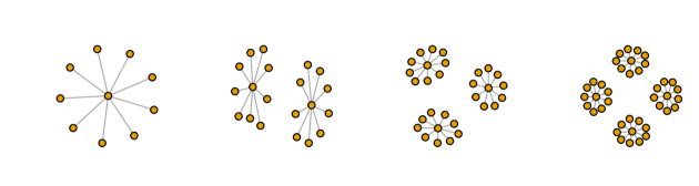
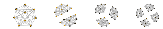
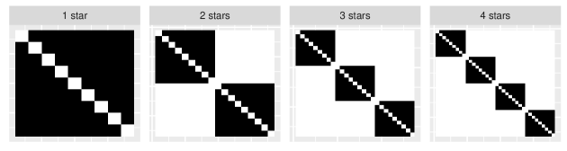
Figure 7: Top row: Graphs of 1 to 4 disjoint stars. Recall the graphon $W=0$ for star graphs. Middle row: Line graphs of disjoint stars in top row. Line graphs of star graphs are complete graphs. Bottom row: The empirical graphons of the line graphs $U_{H_{m}}$ of the star graphs shown on top.

4.2.1 Single star graphs

Since the star graph $K_{1,n}$ is sparse, a sequence of star graphs converges to graphon $W=0$. In the following lemma, we show that the corresponding sequence of line graphs $H_{m}=L(G_{n})$ converge to a non-zero graphon $U$.

Lemma 4.2.

The line graphs $\{H_{m}\}_{m}$ of a sequence of star graphs $\{{K_{1,n-1}}\}_{n}$ converge to the graphon $U$ where $U(x,y)=1$ almost everywhere.

Proof.

For $n\geq 2$ we consider the line graphs $H_{m}=L(K_{1,n-1})$ of this sequence. The line graph $H_{m}$ of a star graph $K_{1,n-1}$ is a complete graph $K_{n-1}$ (Lemma 2.3-6). We obtain the empirical graphon (Definition 2.9) of $H_{m}$ by splitting the interval $[0,1]$ into $m$ equal intervals $\{I_{1},I_{2},\ldots,I_{m}\}$ and for $x\in I_{i},y\in I_{j}$ have

$$U_{H_{m}}(x,y)=\begin{cases}0\quad\text{if}\quad i=j\,,\\ 1\quad\text{otherwise}\end{cases}\,.$$

The empirical graphon $U_{H_{m}}$ is illustrated in the bottom leftmost diagram in Figure 7. Consider $U(x,y)=1$ for all $x,y$. The cut norm (Definition 2.5) of $\lVert U_{H_{m}}-U\rVert_{\square}$ is

$$\lVert U_{H_{m}}-U\rVert_{\square}=\sup_{S,T}\left|\int_{S\times T}U_{H_{m}}(x,y)-U(x,y)\,dxdy\right|\,\,.$$

Using the intervals $\{I_{1},I_{2},\ldots,I_{m}\}$ and for $x\in I_{i},y\in I_{j}$ we have

$$U(x,y)-U_{H_{m}}(x,y)=\begin{cases}1\quad\text{if}\quad i=j\,,\\ 0\quad\text{otherwise}\end{cases}\,,$$

giving

$$\lVert U_{H_{m}}-U\rVert_{\square}=\frac{1}{m^{2}}\times m=\frac{1}{m}\,,$$

as each $I_{i}\times I_{i}$ square would give rise to $\frac{1}{m^{2}}$ area. We have used $S=T=[0,1]$ as any $S\subset[0,1]$ and $T\subset[0,1]$ would give smaller area. The cut metric (Definition  2.6)

$$\delta_{\square}(U_{H_{m}},U)=\inf_{\varphi}\left\lVert U_{H_{m}}-U^{\varphi}\right\rVert_{\square}=\lVert U_{H_{m}}-U\rVert_{\square}\,,$$

as $U^{\varphi}=U$ when $U(x,y)=1$. As $\lim_{m\to\infty}\lVert U_{H_{m}}-U\rVert_{\square}=0$, we have

$$\lim_{m\to\infty}\delta_{\square}(U_{H_{m}},U)=0\,,$$

and from Theorem 2.11 (Borgs et al., 2011) $\{H_{m}\}_{m}$ converges to $U$. We note that this works for any $U(x,y)=1$ almost everywhere. ∎

4.2.2 Multiple stars

Next we consider $k$ disjoint stars denoted by $G_{n_{i}}=\{K_{1,s_{1}},K_{1,s_{2}},\ldots,K_{1,s_{k}}\}$ and the sequence $\{G_{n_{i}}\}_{i}$ as follows: When $i=1$ we start with $k$ nodes each denoting the centre of a star. Let $\{r_{1},\ldots,r_{k}\}$ denote positive integers and let $R=\sum_{j}r_{j}$. At each step we add $R$ nodes to the graph. Of the $R$ nodes, $r_{j}$ nodes connect to $K_{1,s_{j}}$ for $j\in\{1,\ldots k\}$. This process results in $k$ disjoint stars with the $j^{\mathrm{th}}$ star having $1+ir_{j}$ nodes at the $i^{\mathrm{th}}$ step. The node ratios converge to $r_{1}\colon r_{2}\colon\ldots\colon r_{k}$ as $i$ goes to infinity. The following lemma shows that the line graphs of disjoint stars converge to an almost block diagonal graphon.

Lemma 4.3.

Let $\{G_{n_{i}}\}_{i}$ denote a disjoint set of $k$ star graphs $\{K_{1,s_{1}},K_{1,s_{2}},\ldots,K_{1,s_{k}}\}$ where $G_{n_{i}}$ has $n_{i}$ vertices and the number of degree-1 vertices of the stars satisfy the ratio $r_{1}\colon r_{2}\colon\ldots\colon r_{k}$ where each $r_{j}\in\mathbb{Z}^{+}$. Consider the graphon $U$ obtained by splitting the interval $[0,1]$ into $k$ sub intervals $\{I_{1},I_{2},\ldots,I_{k}\}$ such that the length of $I_{r}$ denoted by $L(I_{r})$ satisfies the following: $L(I_{1})\colon L(I_{2})\colon\ldots\colon L(I_{k})=r_{1}\colon r_{2}\colon\ldots\colon r_{k}$ and for $x\in I_{i}$ and $y\in I_{j}$

$$U(x,y)=\begin{cases}1&\quad\text{if}\quad i=j\\ 0&\quad\text{otherwise}\end{cases}\,,$$

making $U$ is a block diagonal graphon. Then, the corresponding line graphs $\{H_{m_{i}}\}_{i}$ where $H_{m_{i}}=L(G_{n_{i}})$ converge to the graphon $U$.

Remark 4.4.

Both single stars and multiple disjoint stars $\{G_{n}\}_{n}$ give rise to $W=0$. However their line graphs $\{H_{m}\}_{m}$ give rise to different graphons $U$ as shown in Lemmas 4.2 and 4.3. This is an example of differentiating sparse graphs in the line graph space. See Figure 7.

4.3 Line graphs of some dense and sparse graphs

Next, we go through some well known graphs and compute their line graph edge densities. We consider specific examples of graph sequences $\{G_{n}\}_{n}\in D$, and $\{G_{n}\}_{n}\in S\backslash S_{q}$.

Theorem 4.5.

Let $\{G_{n}\}_{n}$ be a sequence of graphs where $G_{n}$ has $n$ vertices and $m$ edges. Let $H_{m}=L(G_{n})$ and suppose $m\to\infty$ as $n\to\infty$. Then $\{G_{n}\}_{n}$ with properties described below give rise to following line graph edge densities.

1. Suppose $G_{n}$ is the complete graph $K_{n}$. Then the edge density of the corresponding line graph, $\text{density}(H_{m})=\frac{4}{n+1}$ and $\lim_{m\to\infty}\text{density}(H_{m})=0$. Furthermore, $\{K_{n}\}_{n}\in D$ and $\{H_{m}\}_{m}\in S$.

2. Suppose $G_{n}$ is an $r$-regular graph. Then the edge density $\text{density}(H_{m})=\frac{4(r-1)}{rn-2}$ and $\lim_{m\to\infty}\text{density}(H_{m})=0$. Furthermore $\{G_{n}\}_{n},\{H_{m}\}_{m}\in S\backslash S_{q}$.

3. Suppose $G_{n}$ is a path. Then the edge density $\text{density}(H_{m})=\frac{2}{n-1}$ and $\lim_{m\to\infty}\text{density}(H_{m})=0$. Furthermore $\{G_{n}\}_{n},\{H_{m}\}_{m}\in S\backslash S_{q}$.

4. Suppose $G_{n}$ is a cycle. Then the edge density $\text{density}(H_{m})=\frac{2}{n-1}$ and $\lim_{m\to\infty}\text{density}(H_{m})=0$. Furthermore $\{G_{n}\}_{n},\{H_{m}\}_{m}\in S\backslash S_{q}$.

4.4 Empirical Experiments on Estimating Graphons

In this section we compare graphs generated from different empirical graphons. Let $G_{n}$ denote a star $K_{1,n-1}$ with $n$ vertices and let $H_{m}=L(G_{n})$. We consider the empirical graphons (see Definition 2.9) $W_{G_{n}}$ and $U_{H_{m}}$ where we consistently use $W$ and $U$ to denote graphons related to $G_{n}$ and $H_{m}$ respectively. We consider the set of $k$ disjoint stars as illustrated in Figure 7. We want to evaluate how well these empirical graphons can generate graphs with $kn$ vertices where $n=100$ and $k\in\{2,3,4,5\}$. That is, do graphs generated from $W_{G_{n}}$ resemble stars when $n$ increases? Similarly, do graphs generated from $U_{H_{m}}$ resemble line graphs of stars when $m$ increases?

To evaluate this, we generate (following Definition 2.7) $W$-random graphs from $W_{G_{n}}$ and $U$-random graphs $U_{H_{m}}$ with $kn$ vertices i.e., let $\hat{G}_{W}=\mathbb{G}(kn,W_{G_{n}})$ and $\hat{H}_{U}=\mathbb{G}(kn,U_{H_{m}})$. Noting we cannot compare $\hat{G}_{W}$ and $\hat{H}_{U}$ because $\hat{G}_{W}$ is in the space of original graphs whereas $\hat{H}_{U}$ is in the space of line-graphs, we consider the line graph of $\hat{G}_{W}$, that is, let $\hat{H}_{W}=L(\hat{G}_{W})$. Then we have 3 graphs in the line graph space, the actual line graph $H=L(G_{kn})$, the estimated line graph of the $W$-random graph $\hat{H}_{W}$ and the estimated $U$-random graph $\hat{H}_{U}$. We compare different quantities derived from $H$, $\hat{H}_{W}$ and $\hat{H}_{U}$ for different $k$. These include the edge-density, the triangle-density, and the cosine similarity of the degree distributions of $\hat{H}_{U}$ and $\hat{H}_{W}$ with $H$.

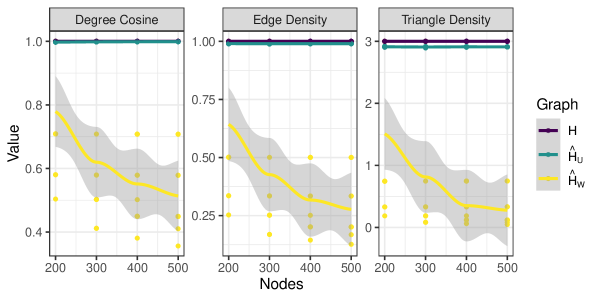
Figure 8: Experiment with 1 star graph. Degree cosine similarity, edge density and triangle density for $H$, $\hat{H}_{U}$ and $\hat{H}_{W}$.

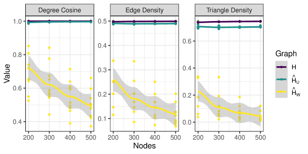
Figure 9: Experiment with 2 star graphs. Degree cosine similarity, edge density and triangle density for $H$, $\hat{H}_{U}$ and $\hat{H}_{W}$.

Figure 8 shows the values obtained from $\hat{H}_{U}$, $\hat{H}_{W}$ and $H$ for a single star graph and Figure 9 shows the metrics for 2 stars. All 3 metrics are better for $\hat{H}_{U}$ compared to $\hat{H}_{W}$. Interestingly, the edge and triangle densities of $\hat{H}_{U}$ are slightly lower than those of $H$ in all instances. This is because $\hat{H}_{U}$ is sampled from $U_{H_{m}}$ which has empty squares along the diagonal, which are effectively closed or blacked out in the graphon $U$ (see empirical graphons in Figure 7). In these two scenarios we know that the shaded-area of $U_{H_{m}}$ is less than that of $U$, and as such slightly lower edge and triangle densities are expected.

5 Results on probabilistic graphs

5.1 Superlinear preferential attachment graphs

Preferential attachment models (Albert & Barabási, 2002) consider nodes connecting to more connected nodes with higher probability. Specifically the probability $\Pi(i)$ that a new node connects to node $i$, which has degree $k_{i}$ is given by

$$\Pi(i)=\frac{k_{i}^{\alpha}}{\sum_{i}k_{i}^{\alpha}}\,,$$ (7)

where $\alpha$ is a parameter. The three regimes $\alpha<1$, $\alpha=1$ and $\alpha>1$ are called sublinear, linear and superlinear preferential attachment respectively. Suppose we start with $s_{0}$ nodes and $s_{0}$ edges and at each time step $t$ a new node is added to the network with $s$ edges. After $t$ timesteps the network has

$$n=t+s_{0}\quad\text{nodes and }\quad m=s_{0}+ts\quad\text{edges.}$$ (8)

For growing networks with superlinear preferential attachment Krapivsky & Redner (2001); Krapivsky et al. (2000) state that the maximum degree $k_{\max}$ satisfies

$$k_{\max}\sim n\,.$$

Sethuraman & Venkataramani (2019) prove a more rigorous version of the above statement. They show that,

$$P\left[\lim_{n\to\infty}\frac{1}{n}k_{\max}=1\right]=1\,.$$

We will use this result to show that superlinear preferential attachment graphs satisfy the square-degree property almost surely.

Lemma 5.1.

Let $\{G_{n}\}_{n}$ denote a sequence of graphs growing by superlinear preferential attachment satisfying equation (7) with $\alpha>1$. Then $\{G_{n}\}_{n}\in S_{q}$ almost surely.

Proof.

Using the result from Sethuraman & Venkataramani (2019) we know that for every $\epsilon>0$ there exists $N_{0}\in\mathbb{N}$ such that

$$P\left[\left|\frac{1}{n}k_{\max}-1\right|<\epsilon\right]=1\,,$$

for all $n>N_{0}$. That is, almost surely

$$1-\epsilon<\frac{1}{n}k_{\max}<1+\epsilon\,,$$

for $n>N_{0}$. Rearranging the equations for $n$ and $m$ (equation (8)) we get $ns=m+(s-1)s_{0}$ giving us $ns>m$. Hence,

$$\sum(\text{deg }v_{i}^{2})>k_{\max}^{2}>(1-\epsilon)^{2}n^{2}>\frac{(1-\epsilon)^{2}m^{2}}{s^{2}}\quad\text{almost surely.}$$

Thus, for $n>N_{0}$

$$P\left[\sum(\text{deg }v_{i}^{2})>\frac{(1-\epsilon)^{2}}{s^{2}}m^{2}\right]=1$$

showing that superlinear preferential attachment graphs satisfy the square-degree property (Definition 3.3) almost surely for large values of $n$. From Theorem 3.6 they produce dense line graphs. If $\{t(F,H_{m})\}_{m}$ converges for all graphs $F$, where $H_{m}=L(G_{n})$ then Theorem 2.10 (Borgs et al., 2008) ensures $\{H_{m}\}_{m}$ converges to a graphon $U$. As $\{H_{m}\}_{m}$ is dense $U\neq 0$. ∎

5.2 Erdős–Rényi graphs

The Erdős–Rényi model $G(n,p)$ describes graphs of $n$ vertices with edge probability $p$, where $p$ is a parameter. Each edge is equally likely to be included in the graph. The degree distribution for any vertex in $G_{n}\sim G(n,p)$ is binomial with parameters $n-1$ and $p$. For a given $n$ and $p$ there exists a graph distribution as different edges can be included or left out in different graphs. Expectations are calculated with respect to this graph distribution.

Theorem 5.2.

Let $G_{n}$ be an Erdős–Rényi graph sampled from a $G(n,p)$ model and suppose $G_{n}$ has $n$ nodes and $m$ edges. Let $H_{m}=L(G_{n})$. As $n$ and $m$ go to infinity, the edge density of $H_{m}$ satisfies

$$\lim_{m\to\infty}P\left[\text{density}(H_{m})=0\right]=1\,.$$ (9)

6 Conclusions

Graphons are a compact representation or a graph model that can generate arbitrarily large graphs. The standard construction of the graphon is useful for dense graphs, but sparse graphs converge to the zero graphon, limiting its utility. The classical construction concerns the non-zero area of the graphon, which is zero for sparse graphs. To overcome this limitation, methods have been proposed that can capture and differentiate point masses, a feature of sparse graphs. Typically, these methods have strong measure-theoretic underpinnings and often involve complex mathematical machinery. In this paper, we show that for a subset of sparse graphs, taking the line graph gives promising results. We propose a condition on sparse graphs, called the square-degree property, which results in dense line graphs. This enables standard graph convergence to be used to analyse graph limits.

We show that graphs that satisfy the square-degree property are sparse, but map to dense line graphs, while graphs that do not satisfy the square-degree property give rise to sparse line graphs. Using the square degree property, we illustrate three cases. First we show that star graphs are sparse and converge to the zero graphon ($W=0$). However, line graphs of star graphs are complete and converge to the graphon $U=1$. Similarly, multiple star graphs converge to $W=0$, but their line graphs converge to a block diagonal graphon $U\neq 0$. Thus, line graphs of multiple star graphs (since they satisfy the the square-degree property) are dense, making the graphon of these line graphs non-zero when convergence exists. Second we show that preferential attachment models give rise to graph sequences that satisfy the square degree property, and hence result in line graphs that converge to non-zero graphons. Third we prove that Erdős–Rényi graphs almost surely give rise to sparse line graphs. We hope that this new approach of using line graphs to analyse graph limits provides an interesting tool for researchers working on graphons.

Appendix A Proofs of lemmas and theorems

See 3.5

Proof.

As $D\subset\bar{S}$, where $\bar{S}$ denotes the complement of $S$, this is true because of the contrapositive of Lemma 3.4. It can be quickly verified that dense graph sequences do not satisfy equation (2) in Lemma 3.4 because for dense graphs $m\geq cn^{2}$ for some $c>0$. ∎

See 3.7

Proof.

The first part is the contra-positive of Theorem 3.6(2). We prove it from first principles for the sake of completeness. Let us restate the square-degree property and consider its negation. If a graph sequence $\{G_{n}\}_{n}$ satisfies the square-degree property, then there exists constants $c_{1}\in(0,1)$ and $N_{0}\in\mathbb{N}$ such that for all $n\geq N_{0}$ we have

$$\sum\text{deg }v_{i,n}^{2}\geq c_{1}\left(\sum\text{deg }v_{i,n}\right)^{2}\,.$$

The negation of square-degree property, $\neg Sq$ says that for all $c_{1}>0$ and $N_{0}\in\mathbb{N}$ there exists $n\geq N_{0}$ such that

$$\sum\text{deg }v_{i,n}^{2}<c_{1}\left(\sum\text{deg }v_{i,n}\right)^{2}\,.$$

For every $N_{0}\in\mathbb{N}$ there exists $n\geq N_{0}$ such that this inequality is satisfied. Consider

$$A_{c_{1}}=\left\{n\in\mathbb{N}:n\geq N_{0},\sum\text{deg }v_{i,n}^{2}<c_{1}\left(\sum\text{deg }v_{i,n}\right)^{2}\right\}\,.$$

If $|A_{c_{1}}|$ was finite, then we can pick $N_{\nu}=\max(A_{c_{1}})+1$ and for $n\geq N_{\nu}$ the inequality $\sum\text{deg }v_{i,n}^{2}<c_{1}\left(\sum\text{deg }v_{i,n}\right)^{2}$ would not be satisfied. Thus, the set $A_{c_{1}}$ has infinitely many elements. Therefore for every $c_{1}\in(0,1)$ and $N_{0}\in\mathbb{N}$ there is an infinite sequence $A_{c_{1}}$ such that for any $n\in A_{c_{1}}$

$$\sum\text{deg }v_{i,n}^{2}<c_{1}\left(\sum\text{deg }v_{i,n}\right)^{2}\,.$$

Hence we can consider a sequence of sequences $\{A_{c_{1_{i}}}\}_{c_{1_{i}}}$ where $c_{1_{i}}>c_{1_{j}}$ when $i<j$. From this sequence set we can choose a diagonal subsequence $\{n_{1},n_{2},\ldots\}$ such that $n_{1}\in A_{c_{1_{1}}}$ and $n_{2}\in A_{c_{1_{2}}}$ and so on, such that this sequence converges to zero. From equation (1) recall that

$$\text{density}(H_{m})=\frac{\frac{1}{2}\sum_{i}(\text{deg }\,v_{i,n})^{2}-m}{\frac{1}{2}m(m-1)}\,.$$

For the diagonal subsequence selected above

$$\frac{\sum\text{deg }v_{i,n}^{2}}{\left(\sum\text{deg }v_{i,n}\right)^{2}}=\frac{\sum\text{deg }v_{i,n}^{2}}{4m^{2}}\to 0\,,$$

giving us

$$\liminf_{m\to\infty}\text{density}(H_{m})=0\,.$$

If $\{H_{m}\}_{m}$ is convergent, then all subsequences converge to the same limit and we get

$$\lim_{m\to\infty}\text{density}(H_{m})=0\,.$$

∎

See 3.8

Proof.

From Definition 2.4

$$t(F,H_{m})=\sum_{\phi:V(F)\to V(H_{m})}\prod_{ij\in E(F)}\beta_{\phi(i)\phi(j)}(H_{m})\cdot\frac{1}{m^{|V(F)|}}\,,\\$$ (10)

where $\phi$ is a mapping from $V(F)$ to $V(H_{m})$ and $\beta_{ij}(H_{m})$ denotes the weight of edge $ij$ in graph $H_{m}$, which is either 1 or 0. Thus,

$$t(\leavevmode\hbox to10.46pt{\vbox to4pt{\text{[drawing]}}},H_{m}) =\sum_{\phi:V(\leavevmode\hbox to8.52pt{\vbox to4pt{\text{[drawing]}}})\to V(H_{m})}\prod_{ij\in E(\leavevmode\hbox to8.52pt{\vbox to4pt{\text{[drawing]}}})}\beta_{\phi(i)\phi(j)}(H_{m})\cdot\frac{1}{m^{2}}\,,$$ (11)

$$=\sum_{\begin{subarray}{c}\phi:V(\leavevmode\hbox to8.52pt{\vbox to4pt{\text{[drawing]}}})\to V(H_{m})\\ ij\in E(\leavevmode\hbox to8.52pt{\vbox to4pt{\text{[drawing]}}})\end{subarray}}\beta_{\phi(i)\phi(j)}(H_{m})\cdot\frac{1}{m^{2}}\,,$$ (12)

where we have dropped the product term as there is only one edge. We can replace the edge weight $\beta_{\phi(i)\phi(j)}(H_{m})$ with the associated value in the empirical graphon $U_{m}(q_{\phi(i)},q_{\phi(j)})$ giving us

$$t(\leavevmode\hbox to10.46pt{\vbox to4pt{\text{[drawing]}}},H_{m}) =\sum_{\begin{subarray}{c}\phi:V(\leavevmode\hbox to8.52pt{\vbox to4pt{\text{[drawing]}}})\to V(H_{m})\\ ij\in E(\leavevmode\hbox to8.52pt{\vbox to4pt{\text{[drawing]}}})\end{subarray}}U_{m}(q_{\phi(i)},q_{\phi(j)})\cdot\frac{1}{m^{2}}\,,$$ (13)

$$=\sum_{i,j}U_{m}(q_{i},q_{j})\cdot\frac{1}{m^{2}}\,,$$ (14)

as $\phi$ can map the edge to any two vertices in $H_{m}$. Every edge in $G_{n}$ is mapped to a vertex in $H_{m}$ and 2 vertices in $H_{m}$ are connected if the corresponding edges in $G_{n}$ have a common vertex. That is, $L(\leavevmode\hbox to12.61pt{\vbox to8.27pt{\text{[drawing]}}})=\leavevmode\hbox to10.46pt{\vbox to4pt{\text{[drawing]}}}$, and for every edge in $H_{m}$ there is a corresponding set of two edges with a common vertex ( ) in $G_{n}$. As a result the empirical graphon (Definition 2.9),

$$U_{m}(q_{i},q_{j})=1\quad\text{if and only if}\quad W_{n}(r_{k},r_{\ell})W_{n}(r_{\ell},r_{s})=1$$

for some $k,\ell,s\in\{1,\ldots,n\}$ with $k\neq s$. The reason $k\neq s$ is because we need 2 distinct edges in $G_{n}$ with a common vertex to make an edge in $H_{m}$. As a result of this one-to-one and onto mapping we have

$$\sum_{i,j}U_{m}(q_{i},q_{j})=\sum_{\begin{subarray}{c}k,\ell,s\\ k\neq s\end{subarray}}W_{n}(r_{k},r_{\ell})W_{n}(r_{\ell},r_{s})\,$$ (15)

giving us the desired result. ∎

See 3.9

Proof.

As $\{G_{n}\}_{n}$ is a dense graph sequence converging to $W$

$$\lim_{n\to\infty}t(\leavevmode\hbox to10.46pt{\vbox to4pt{\text{[drawing]}}}\,,G_{n})=\lim_{n\to\infty}\frac{2m}{n^{2}}=c>0\,.$$ (16)

We will use this limit later. Let $W_{n}$ be the empirical graphon of $G_{n}$ with $[0,1]$ divided into $n$ equal intervals $\{r_{1},\ldots r_{n}\}$ and let $U_{m}$ be the empirical graphon of $H_{m}$ with $[0,1]$ equally divided into $m$ intervals $\{q_{1},\ldots,q_{m}\}$. The homomorphism density $\{t(\leavevmode\hbox to12.61pt{\vbox to8.27pt{\text{[drawing]}}},G_{n})\}_{n}$ is a converging sequence as $\{G_{n}\}_{n}$ converges to $W$. We have

$$t(\leavevmode\hbox to12.61pt{\vbox to8.27pt{\text{[drawing]}}},G_{n})=\sum_{\begin{subarray}{c}i,j,k\end{subarray}}W(r_{i},r_{k})W(r_{k},r_{j})\cdot\frac{1}{n^{3}}\,,$$

converging as $n$ goes to infinity. From Lemma 3.8 we know

$$t(\leavevmode\hbox to10.46pt{\vbox to4pt{\text{[drawing]}}},H_{m}) =\sum_{\begin{subarray}{c}i,j\end{subarray}}U(q_{i},q_{j})\cdot\frac{1}{m^{2}}\,,$$ (17)

$$=\sum_{\begin{subarray}{c}i,j,k\\ i\neq j\end{subarray}}W(r_{i},r_{k})W(r_{k},r_{j})\cdot\frac{1}{m^{2}}\,,$$ (18)

$$\leq\sum_{\begin{subarray}{c}i,j,k\end{subarray}}W(r_{i},r_{k})W(r_{k},r_{j})\cdot\frac{1}{m^{2}}\,,$$ (19)

$$=\sum_{\begin{subarray}{c}i,j,k\end{subarray}}\frac{1}{n^{4}}W(r_{i},r_{k})W(r_{k},r_{j})\cdot\frac{1}{\left(\frac{m}{n^{2}}\right)^{2}}\,.$$ (20)

As $n$ and $m$ go to infinity we get

$$\limsup_{m\to\infty}t(\leavevmode\hbox to10.46pt{\vbox to4pt{\text{[drawing]}}},H_{m})=\lim_{\begin{subarray}{c}n\to\infty\\ m\to\infty\end{subarray}}\frac{1}{n}\cdot t(\leavevmode\hbox to12.61pt{\vbox to8.27pt{\text{[drawing]}}},G_{n})\cdot\frac{1}{\left(\frac{m}{n^{2}}\right)^{2}}=0\,,$$

as $m/n^{2}$ goes to $c/2>0$ (equation (16)) and $t(\leavevmode\hbox to12.61pt{\vbox to8.27pt{\text{[drawing]}}},G_{n})$ converges. As $t(\leavevmode\hbox to10.46pt{\vbox to4pt{\text{[drawing]}}},H_{m})$ lies between $0$ and $1$ we get

$$\lim_{m\to\infty}t(\leavevmode\hbox to10.46pt{\vbox to4pt{\text{[drawing]}}},H_{m})=0\,.$$

As $t(\leavevmode\hbox to10.46pt{\vbox to4pt{\text{[drawing]}}},H_{m})=\frac{2m^{\prime}}{n^{\prime 2}}$ goes to 0, where $m^{\prime}$ and $n^{\prime}$ denote the number of edges and vertices in $H_{m}$, the cut-norm (Definition 2.5) satisfies

$$\lVert U_{H_{m}}-U\rVert_{\square}=\lVert U_{H_{m}}\rVert_{\square}=\frac{2m^{\prime}}{n^{\prime}(n^{\prime}-1)}\rightarrow 0\,,$$

where $U(x,y)=0$. As the cut-metric (Definition 2.6)

$$\delta_{\square}\left(U_{H_{m}},U\right)=\inf_{\varphi}\lVert U_{H_{m}}-U^{\varphi}\rVert\,,$$

$\{H_{m}\}_{m}$ converges to $U$ in the cut-metric as the infimum is considered and as $U^{\varphi}=U$ for $U=0$. ∎

See 3.10

Proof.

From Theorem 3.6 we know $\{G_{n}\}_{n}\in S_{q}\equiv\{H_{m}\}_{m}\in D$. Additionally, if $\{H_{m}\}_{m}$ converges to $U$ then $\{t(\leavevmode\hbox to10.46pt{\vbox to4pt{\text{[drawing]}}},H_{m})\}_{m}$ converges to $t(\leavevmode\hbox to10.46pt{\vbox to4pt{\text{[drawing]}}},U)$. As $t(\leavevmode\hbox to10.46pt{\vbox to4pt{\text{[drawing]}}},H_{m})=\frac{2m^{\prime}}{n^{\prime 2}}$ where $m^{\prime}$ and $n^{\prime}$ denote the number of edges and nodes in $H_{m}$ where $n^{\prime}=m$, the sequence $\frac{2m^{\prime}}{n^{\prime 2}}$ converges to some constant $c$. But as $\{H_{m}\}_{m}\in D$

$$t(\leavevmode\hbox to10.46pt{\vbox to4pt{\text{[drawing]}}},U)=\lim_{n^{\prime}\to\infty}\frac{2m^{\prime}}{n^{\prime 2}}=c>0\,,$$

that is, the edge density of $\{H_{m}\}_{m}$ converges to a positive constant. The homomorphism density $t(\leavevmode\hbox to10.46pt{\vbox to4pt{\text{[drawing]}}},U)$ (Definition 2.4) is given by

$$t(\leavevmode\hbox to10.46pt{\vbox to4pt{\text{[drawing]}}},U)=\int_{[0,1]^{2}}U(x,y)\,dxdy\,,$$

which is equal to the cut-norm of $U$

$$\lVert U\rVert_{\square}=\sup_{S,T}\left|\int_{S\times T}U(x,y)dxdy\right|\,,$$

because $U(x,y)\in[0,1]$ and the supremum is achieved when $S=T=[0,1]$, giving us

$$\lVert U\rVert_{\square}=t(\leavevmode\hbox to10.46pt{\vbox to4pt{\text{[drawing]}}},U)>0\,.$$

∎

See 3.11

Proof.

As $\{G_{n}\}_{n}\in S$, it is sparse and it converges to $W=0$. From Lemma 3.7  if $\{G_{n}\}_{n}\notin S_{q}$

$$\liminf_{m\to\infty}\text{density}(H_{m})=0\,.$$

As $\{H_{m}\}_{m}$ converges to $U$, the edge densities converge and we get $\lim_{m\to\infty}\text{density}(H_{m})=0$. The empirical graphon $U_{H_{m}}$ converges to $U$ and we have the cut norm (Definition 2.5) of the empirical graphon

$$\lVert U_{H_{m}}\rVert=\frac{2m^{\prime}}{n^{\prime}(n^{\prime}-1)}\to 0$$

giving us

$$\lim_{m\to\infty}\lVert U_{H_{m}}-U\rVert=0\,,$$

where $U=0$. As the cut-metric (Definition 2.6)

$$\delta_{\square}\left(U_{H_{m}},U\right)=\inf_{\varphi}\lVert U_{H_{m}}-U^{\varphi}\rVert\,,$$

we get the result. ∎

See 3.12

Proof.

For converging sequences $\{G_{n}\}_{n}$ and $\{H_{m}\}_{m}$ we have $W=0$ or $U=0$ (Lemmas 3.9, 3.10 and 3.11). The graphon $W\neq 0$ only when $\{G_{n}\}_{n}\in D$. When $\{G_{n}\}_{n}\in D$ we have $\{H_{m}\}_{m}\in S$ giving $U=0$. The graphon $U\neq 0$ only when $\{G_{n}\}_{n}\in S_{q}$ implying $W=0$ as $S_{q}\subset S$. ∎

See 4.1

Proof.

We present an alternate proof from first principles. For the sake of completeness, we do the computation from first principles. For a star graph

$$\text{deg }v_{i}=\begin{cases}n-1\quad\text{ for star vertex }\,,\\ 1\quad\text{otherwise}\end{cases}$$

giving us

$$\sum\text{deg }v_{i,n}^{2} =(n-1)^{2}+1+\cdots+1\,,$$

$$=(n-1)^{2}+(n-1)\,,$$

$$\sum\text{deg }v_{i,n} =m=n-1\,,$$

$$\frac{\sum\text{deg }v_{i,n}^{2}}{\left(\sum\text{deg }v_{i,n}\right)^{2}} =1+\frac{1}{n-1}>1\,,$$

showing that $\{K_{1,n}\}_{n}\in S_{q}$ (Definition 3.3). From equation (1), the density of $H_{m}$ is given by

$$\text{density}(H_{m}) =\frac{\frac{1}{2}\sum_{i}(\text{deg }\,v_{i,n})^{2}-m}{\frac{1}{2}m(m-1)}\,,$$

$$=\frac{\frac{1}{2}((n-1)^{2}+1+1+\ldots+1)-(n-1)}{\frac{1}{2}(n-1)(n-2)}\,,$$

$$=\frac{\frac{1}{2}((n-1)^{2}+(n-1))-(n-1)}{\frac{1}{2}(n-1)(n-2)}\,,$$

$$=\frac{\frac{1}{2}(n-1)(n)-(n-1)}{\frac{1}{2}(n-1)(n-2)}\,,$$

$$=\frac{\frac{1}{2}(n-1)(n-2)}{\frac{1}{2}(n-1)(n-2)}\,,$$

$$=1\,.$$

Thus, $\lim_{m\to\infty}\text{density}(H_{m})=1$. ∎

See 4.3

Proof.

The line graph of $k$ disjoint stars is $k$ disjoint complete subgraphs. This follows from Lemma 2.3 (4 and 6) as vertices of 2 different stars are not connected. Noting $H_{m_{i}}$ has $m_{i}$ vertices, we obtain the empirical graphon (Definition 2.9) of $H_{m_{i}}$ by splitting the interval $[0,1]$ into $m_{i}$ equal intervals $\{I_{1},I_{2},\ldots,I_{m_{i}}\}$.

At the $i$th step, the $j$th star $K_{1,s_{j}}$ has $1+ir_{j}$ nodes and $ir_{j}$ edges. Then the corresponding complete subgraph $K_{s_{j}}$ of the line graph $H_{m_{i}}$ has $ir_{j}$ nodes as each node in the line graph corresponds to an edge in $G_{n_{i}}$. We label nodes belonging to a complete subgraph consecutively. That gives us vertices $1,\ldots,ir_{1}$ corresponding to the first complete subgraph $K_{s_{1}}$, and nodes $(ir_{1}+1),\ldots,(ir_{1}+ir_{2})$ corresponding the second complete subgraph $K_{s_{2}}$ and so on. The ratio between the number of nodes in each subgraph is $r_{1}:r_{2}:\ldots:r_{k}$.

Let us group the vertices in $H_{m}$, $\{1,2,\ldots,{m_{i}}\}$ into $k$ groups $\{J_{1},J_{2},\ldots,J_{k}\}$ according to the complete subgraph they belong to. Then for $x\in I_{j},y\in I_{h}$ we have the empirical graphon (Definition 2.9) of $H_{m}$

$$U_{H_{m_{i}}}(x,y)=\begin{cases}1\quad\text{if}\quad j,h\in J_{\ell}\text{ for some }\ell\text{ but }j\neq h\\ 0\quad\text{if}\quad j=h\text{ as there are no loops}\\ 0\quad\text{if}\quad j\in J_{p}\text{ and }h\in J_{q}\text{ where }p\neq q\end{cases}\,.$$

The bottom row in Figure 7 shows empirical graphons for $k\in\{2,3,4\}$. Note that $U$ is a block diagonal graphon similar to $U_{H_{m_{i}}}$ differing to $U_{H_{m_{i}}}$ only on the diagonal. One can visualize $U$ by colouring the white squares on the diagonal in empirical graphons in Figure 7 for $k\in\{2,3,4\}$.

Then, the cut-norm (Definition 2.5),

$$\lVert U_{H_{m}}-U\rVert_{\square} =\sup_{S,T}\left|\int_{S\times T}U_{H_{m}}(x,y)-U(x,y)\,dxdy\right|\,\,,$$ (21)

$$=\frac{1}{m_{i}^{2}}\times m_{i}=\frac{1}{m_{i}}\,,$$ (22)

where we have used $S=T=[0,1]$ in computing the cut-norm as any other $S$ or $T$ would give smaller area. Then the cut metric (Definition 2.6)

$$\delta_{\square}(U_{H_{m}},U)=\inf_{\varphi}\left\lVert U_{H_{m}}-U^{\varphi}\right\rVert_{\square}\leq\lVert U_{H_{m}}-U\rVert_{\square}=\frac{1}{m_{i}}\,.$$

As $\lVert U_{H_{m}}-U\rVert_{\square}$ goes to zero as $m$ goes to infinity $\delta_{\square}(U_{H_{m}},U)$ converges to zero. From Theorem 2.11 (Borgs et al. 2011) $\{H_{m_{i}}\}_{m_{i}}$ converges to $U$. ∎

See 4.5

Proof.

Recall that

$$\text{density}(H_{m})=\frac{\frac{1}{2}\sum(\text{deg }\,v^{2})-m}{\frac{1}{2}m(m-1)}\,.$$

1. Suppose $G_{n}$ is the complete graph $K_{n}$. As $\text{density}(K_{n})=1$, the sequence $\{K_{n}\}_{n}$ is dense, i.e, $\{K_{n}\}_{n}\in D$. For $K_{n}$, $\text{deg }v_{i}=n-1$ and $m=n(n-1)/2$ giving us

   $$\text{density}(H_{m}) =\frac{\frac{1}{2}n(n-1)^{2}-\frac{1}{2}n(n-1)}{\frac{1}{2}\frac{1}{2}n(n-1)(\frac{1}{2}n(n-1)-1)}\,,$$

   $$=\frac{\frac{1}{2}n(n-1)(n-1-1)}{\frac{1}{2}\frac{1}{2}n(n-1)\frac{1}{2}(n(n-1)-2)}$$

   $$=\frac{n-2}{\frac{1}{4}(n+1)(n-2)}\,,$$

   $$=\frac{4}{n+1}\,,$$

   $$\text{making}\quad\lim_{m\to\infty}\text{density}(H_{m}) =0\Rightarrow\{H_{m}\}_{m}\in S.$$

2. Suppose $G_{n}$ is an $r$-regular graph. As $n$ grows each $G_{n}$ is connected to $r$ nodes. Then $\text{deg }v_{i}=r$ and $m=rn/2$. The ratio $m/n^{2}=r/2n$ assigning $\{G_{n}\}_{n}\in S$. The density of $H_{m}$ is given by

   $$\text{density}(H_{m}) =\frac{\frac{1}{2}nr^{2}-\frac{1}{2}nr}{\frac{1}{2}\frac{1}{2}rn(\frac{1}{2}rn-1)}\,,$$ (23)

   $$=\frac{\frac{1}{2}rn(r-1)}{\frac{1}{2}\frac{1}{2}rn\frac{1}{2}(rn-2)}\,,$$ (24)

   $$=\frac{4(r-1)}{rn-2}\,.$$ (25)

   Thus, $\lim_{m\to\infty}\text{density}(H_{m})=0$, making both $\{G_{n}\}_{n},\{H_{m}\}_{m}\in S$. Using Theorem 3.6 we can conclude $\{G_{n}\}_{n}\notin S_{q}$ because $\{G_{n}\}_{n}\in S_{q}\iff\{H_{m}\}_{m}\in D$. Hence $\{G_{n}\}_{n}\in S\backslash S_{q}$. As $G$ is an $r$-regular graph, $H$ is a $2(r-1)$-regular graph with $\frac{nr}{2}$ vertices (Lemma 2.3-2). Thus, using the same reasoning we have $\{H_{m}\}_{m}\in S\backslash S_{q}$. This is an example where both graph sequences $\{G_{n}\}_{n}$ and $\{H_{m}\}_{m}$ are sparse and both $\{G_{n}\}_{n},\{H_{m}\}_{m}\in S\backslash S_{q}$.

3. Suppose $G_{n}$ is a path. Then $m=n-1$ and the starting and ending vertices have degree 1 and the rest have degree 2. Thus,

   $$\text{density}(H_{m}) =\frac{\frac{1}{2}(1^{2}+(n-2)2^{2}+1^{2})-m}{\frac{1}{2}m(m-1)}\,,$$

   $$=\frac{\frac{1}{2}(2+4(m-1))-m}{\frac{1}{2}m(m-1)}\,,$$

   $$=\frac{1+2(m-1)-m}{\frac{1}{2}m(m-1)}\,,$$

   $$=\frac{m-1}{\frac{1}{2}m(m-1)}\,,$$

   $$=\frac{2}{m}=\frac{2}{n-1}\,.$$

   Thus, $\lim_{m\to\infty}\text{density}(H_{m})=0$. The edge density can also be derived by recognizing a path of $n$ vertices gives rise to a line graph that is a path of $n-1$ vertices (Lemma 2.3-3). Using the same reasoning as previously for $r$-regular graphs, we can conclude that both $\{G_{n}\}_{n},\{H_{m}\}_{m}\in S\backslash S_{q}$.

4. Suppose $G_{n}$ is a cycle, i.e. $G_{n}=C_{n}$. Then $n=m$ and all vertices have degree 2. This is a 2-regular graph. Using equation (25) we get

   $$\text{density}(H_{m}) =\frac{4(r-1)}{rn-2}\,,$$ (26)

   $$=\frac{4}{2n-2}=\frac{2}{n-1}\,,$$ (27)

   which limits to zero. From Lemma 2.3-5 we know that $L(C_{n})=C_{n}$. Here too both $\{G_{n}\}_{n},\{H_{m}\}_{m}\in S\backslash S_{q}$ as previously.

∎

Lemma A.1.

Consider the graph $G_{n}$ sampled from a $G(n,p)$ model and suppose $G_{n}$ has $n$ nodes and $m$ edges. Let $X_{ij}$ denote the random variable corresponding to the edge between vertices $i$ and $j$, i.e., $X_{ij}=1$ if the edge exists and $0$ otherwise. Let $Y_{j}=\sum_{i}X_{ij}$, $\mu=\mathbb{E}[Y_{j}]$ and $\bar{m}=\mathbb{E}[m]$. Let $Y_{\text{ssq}}=\sum_{j}Y_{j}^{2}$, and $m_{\text{sq}}=m^{2}$. Then for a given $\alpha\in(0,1)$ and $c>0$ we have

$$P\left[Y_{\text{ssq}}\geq cm_{\text{sq}}|m_{\text{sq}}\leq(1-\alpha)^{2}\bar{m}^{2}\right]P\left[m_{\text{sq}}\leq(1-\alpha)^{2}\bar{m}^{2}\right]\leq\exp\left(-\frac{\alpha^{2}pn(n-1)}{4}\right)\,.$$

Proof.

For a given $\alpha\in(0,1)$ we get the following Chernoff-Hoeffding bounds (Frieze & Karoński 2015) for $m$:

$$P\left[m\leq(1-\alpha)\bar{m}\right] \leq\exp\left(-\frac{\alpha^{2}\bar{m}}{2}\right)\,,$$ (28)

$$\text{giving us }\quad P\left[m^{2}\leq(1-\alpha)^{2}\bar{m}^{2}\right] \leq\exp\left(-\frac{\alpha^{2}\bar{m}}{2}\right)\,,$$ (29)

as $m$ is positive. As the probability $P\left[Y_{\text{ssq}}\geq cm_{\text{sq}}|m_{\text{sq}}\leq(1-\alpha)^{2}\bar{m}^{2}\right]\leq 1$, $m_{\text{sq}}=m^{2}$ and $\bar{m}=pn(n-1)/2$ we get the desired result. ∎

Lemma A.2.

Consider the graph $G_{n}$ sampled from a $G(n,p)$ model and suppose $G_{n}$ has $n$ nodes and $m$ edges. Let $X_{ij}$ denote the random variable corresponding to the edge between vertices $i$ and $j$, i.e., $X_{ij}=1$ if the edge exists and $0$ otherwise. Let $Y_{j}=\sum_{i}X_{ij}$, $\mu=\mathbb{E}[Y_{j}]$ and $\bar{m}=\mathbb{E}[m]$. Let $Y_{\text{ssq}}=\sum_{j}Y_{j}^{2}$, and $m_{\text{sq}}=m^{2}$. Then for a given $\alpha\in(0,1)$ and $c>0$ we have

$$P\left[Y_{\text{ssq}}\geq cm_{\text{sq}}|m_{\text{sq}}\geq(1+\alpha)^{2}\bar{m}^{2}\right]P\left[m_{\text{sq}}\geq(1+\alpha)^{2}\bar{m}^{2}\right]\leq\exp\left(-\frac{\alpha^{2}pn(n-1)}{6}\right)\,.$$

Proof.

The proof is similar to Lemma A.1 with the only difference being the Chernoff-Hoeffding bound, which changes to:

$$P\left[m\geq(1+\alpha)\bar{m}\right]\leq\exp\left(-\frac{\alpha^{2}\bar{m}}{3}\right)\,.$$

∎

Lemma A.3.

Consider the graph $G_{n}$ sampled from a $G(n,p)$ model and suppose $G_{n}$ has $n$ nodes and $m$ edges. Let $X_{ij}$ denote the random variable corresponding to the edge between vertices $i$ and $j$, i.e., $X_{ij}=1$ if the edge exists and $0$ otherwise. Let $Y_{j}=\sum_{i}X_{ij}$, $\mu=\mathbb{E}[Y_{j}]$ and $\bar{m}=\mathbb{E}[m]$. Let $Y_{\text{ssq}}=\sum_{j}Y_{j}^{2}$, and $m_{\text{sq}}=m^{2}$. Then for a fixed $c>0$ and fixed $\alpha\in(0,1)$ for $n>\frac{4}{c(1-\alpha)^{2}}$ and $\beta=\frac{\sqrt{cn}(1-\alpha)}{2}-1$ we have

$$P\left[Y_{\text{ssq}}\geq cm_{\text{sq}}|(1-\alpha)^{2}\bar{m}^{2}\leq m_{\text{sq}}\leq(1+\alpha)^{2}\bar{m}^{2}\right] P\left[(1-\alpha)^{2}\bar{m}^{2}\leq m_{\text{sq}}\leq(1+\alpha)^{2}\bar{m}^{2}\right]$$ (30)

$$\leq\exp\left(\ln n-\frac{\beta^{2}p(n-1)}{3}\right)\,.$$ (31)

Proof.

We focus on the term $P\left[Y_{\text{ssq}}\geq cm_{\text{sq}}|(1-\alpha)^{2}\bar{m}^{2}\leq m_{\text{sq}}\leq(1+\alpha)^{2}\bar{m}^{2}\right]$. We know that $\mu=p(n-1)$ and $\bar{m}=pn(n-1)/2$. As $m_{\text{sq}}\in\left[(1-\alpha)^{2}\bar{m}^{2},\,(1+\alpha)^{2}\bar{m}^{2}\right]$ we get

$$P\left[Y_{\text{ssq}}\geq cm_{\text{sq}}|(1-\alpha)^{2}\bar{m}^{2}\leq m_{\text{sq}}\leq(1+\alpha)^{2}\bar{m}^{2}\right] \leq P\left[Y_{\text{ssq}}\geq c(1-\alpha)^{2}\bar{m}^{2}\right]\,,$$ (32)

$$=P\left[Y_{\text{ssq}}\geq c\left(\frac{n\mu}{2}\right)^{2}(1-\alpha)^{2}\right]\,,$$ (33)

$$=P\left[Y_{\text{ssq}}\geq n\mu^{2}(1+\beta)^{2}\right]\,,$$ (34)

where we have substituted $\bar{m}=\frac{n\mu}{2}$ in equation (33) and rearranged the terms for $\beta$. For $n>\frac{4}{c(1-\alpha)^{2}}$, we get $\frac{\sqrt{cn}(1-\alpha)}{2}>1$ making $\beta>0$.

For a given $\beta>0$, we get the following Chernoff-Hoeffding bound for $Y_{j}$:

$$P\left[Y_{j}\geq(1+\beta)\mu\right]\leq\exp\left(-\frac{\beta^{2}\mu}{3}\right)\,.$$ (35)

$$\text{As }Y_{j}\geq 0\text{ we have }\quad P\left[Y_{j}^{2}\geq(1+\beta)^{2}\mu^{2}\right]\leq\exp\left(-\frac{\beta^{2}\mu}{3}\right)\,,$$ (36)

$$\text{and from Boole's inequality}\quad P\left[Y_{\text{ssq}}\geq n(1+\beta)^{2}\mu^{2}\right]\leq n\exp\left(-\frac{\beta^{2}\mu}{3}\right)\,.$$ (37)

Substituting equation (37) in equation (34) we get

$$P\left[Y_{\text{ssq}}\geq cm_{\text{sq}}|(1-\alpha)^{2}\bar{m}^{2}\leq m_{\text{sq}}\leq(1+\alpha)^{2}\bar{m}^{2}\right] \leq n\exp\left(-\frac{\beta^{2}\mu}{3}\right)\,,$$ (39)

$$\leq\exp\left(\ln n-\frac{\beta^{2}\mu}{3}\right)$$ (40)

for $n>\frac{4}{c(1-\alpha)^{2}}$ and $\beta=\frac{\sqrt{cn}(1-\alpha)}{2}-1$. ∎

See 5.2

Proof.

Let $X_{ij}$ denote the Bernoulli random variable corresponding to the edge between nodes $i$ and $j$ in $G_{n}$ and let $X_{ij}=1$ if the edge is present and $0$ otherwise. Let $Y_{j}=\sum_{i}X_{ij}$. Then the degree of each node $j$ in $G_{n}$ is given by $\text{deg }v_{j}=Y_{j}$. Let $\mu=\mathbb{E}[Y_{j}]$ and $\bar{m}=\mathbb{E}[m]$. We know that $\mu=p(n-1)$ and $\bar{m}=pn(n-1)/2$. Let $Y_{\text{ssq}}=\sum_{j}Y_{j}^{2}$, and $m_{\text{sq}}=m^{2}$ where ssq denotes the sum of squares and sq denotes square.

We fix $c$ and $\alpha$ such that $c,\alpha\in(0,1)$ and compute $P\left[Y_{\text{ssq}}\geq cm_{\text{sq}}\right]$ using the law of total probability

$$P\left[Y_{\text{ssq}}\geq cm_{\text{sq}}\right] =P\left[Y_{\text{ssq}}\geq cm_{\text{sq}}|m_{\text{sq}}\leq(1-\alpha)^{2}\bar{m}^{2}\right]P\left[m_{\text{sq}}\leq(1-\alpha)^{2}\bar{m}^{2}\right]+$$ (41)

$$P\left[Y_{\text{ssq}}\geq cm_{\text{sq}}|(1-\alpha)^{2}\bar{m}^{2}\leq m_{\text{sq}}\leq(1+\alpha)^{2}\bar{m}^{2}\right]P\left[(1-\alpha)^{2}\bar{m}^{2}\leq m_{\text{sq}}\leq(1+\alpha)^{2}\bar{m}^{2}\right]+$$ (42)

$$P\left[Y_{\text{ssq}}\geq cm_{\text{sq}}|m_{\text{sq}}\geq(1+\alpha)^{2}\bar{m}^{2}\right]P\left[m_{\text{sq}}\geq(1+\alpha)^{2}\bar{m}^{2}\right]\,,\$$ (43)

$$\leq\exp\left(-\frac{\alpha^{2}pn(n-1)}{4}\right)+\exp\left(\ln n-\frac{\beta^{2}p(n-1)}{3}\right)+\exp\left(-\frac{\alpha^{2}pn(n-1)}{6}\right)\,,$$ (44)

from Lemmas A.1, A.2 and A.3 for $n>\frac{4}{c(1-\alpha)^{2}}$ and $\beta=\frac{\sqrt{cn}(1-\alpha)}{2}-1$.

For a fixed $c\in(0,1)$ we get

$$\lim_{n,m\to\infty}P\left[Y_{\text{ssq}}\geq cm_{\text{sq}}\right]=0$$

As

$$P\left[\frac{1}{2}Y_{\text{ssq}}\geq\frac{1}{2}cm_{\text{sq}}\right]=P\left[\frac{1}{2}\sum_{j}Y_{j}^{2}-m\geq\frac{1}{2}cm^{2}-m\right]$$

For $c\in(0,1)$ we have $\frac{1}{2}cm^{2}-\frac{1}{2}cm>\frac{1}{2}cm^{2}-m$ giving us

$$P\left[\frac{1}{2}\sum_{j}Y_{j}^{2}-m\geq\frac{1}{2}cm^{2}-\frac{1}{2}cm\right]\leq P\left[\frac{1}{2}\sum_{j}Y_{j}^{2}-m\geq\frac{1}{2}cm^{2}-m\right]=P\left[Y_{\text{ssq}}\geq cm_{\text{sq}}\right]\,.$$

As $n$ and $m$ go to infinity

$$\lim_{n,m\to\infty}P\left[\frac{\frac{1}{2}\sum_{j}Y_{j}^{2}-m}{\frac{m(m-1)}{2}}\geq c\right] =0\,.$$ (45)

Using the line graph edge density in equation (1)

$$\lim_{m\to\infty}P\left[\text{density}(H_{m})\geq c\right] =0\,,$$ (47)

giving us the first result. Taking the complement we have

$$\lim_{m\to\infty}P\left[\text{density}(H_{m})<c\right]=1\,,$$

for a fixed $c\in(0,1)$. As this is true for any $c\in(0,1)$ we have

$$\lim_{m\to\infty}P\left[\text{density}(H_{m})=0\right]=1\,.$$

∎

References

- (1)
- Albert & Barabási (2002) Albert, R. & Barabási, A.-L. (2002), ‘Statistical mechanics of complex networks’, Reviews of Modern Physics 74(1), 47.
- Beineke & Bagga (2021) Beineke, L. W. & Bagga, J. S. (2021), Line graphs and line digraphs, Springer.
- Bollobás & Riordan (2011) Bollobás, B. & Riordan, O. (2011), ‘Sparse graphs: Metrics and random models’, Random Structures and Algorithms 39(1), 1–38.
- Borgs, Chayes, Cohn & Zhao (2019) Borgs, C., Chayes, J., Cohn, H. & Zhao, Y. (2019), ‘An theory of sparse graph convergence I: Limits, sparse random graph models, and power law distributions’, Transactions of the American Mathematical Society 372(5), 3019–3062.
- Borgs et al. (2017) Borgs, C., Chayes, J. & Gamarnik, D. (2017), ‘Convergent sequences of sparse graphs: A large deviations approach’, Random Structures and Algorithms 51(1), 52–89.
- Borgs et al. (2011) Borgs, C., Chayes, J., Lovász, L., Sós, V. & Vesztergombi, K. (2011), ‘Limits of randomly grown graph sequences’, European Journal of Combinatorics 32(7), 985–999.
- Borgs et al. (2018) Borgs, C., Chayes, J. T., Cohn, H. & Holden, N. (2018), ‘Sparse exchangeable graphs and their limits via graphon processes’, Journal of Machine Learning Research 18(210), 1–71.
- Borgs, Chayes, Cohn & Veitch (2019) Borgs, C., Chayes, J. T., Cohn, H. & Veitch, V. (2019), ‘Sampling perspectives on sparse exchangeable graphs’, Annals of Probability 47(5), 2754–2800.
- Borgs et al. (2021) Borgs, C., Chayes, J. T., Dhara, S. & Sen, S. (2021), ‘Limits of Sparse Configuration Models and Beyond: Graphexes and Multigraphexes’, Annals of Probability 49(6), 2830–2873.
- Borgs et al. (2008) Borgs, C., Chayes, J. T., Lovász, L., Sós, V. T. & Vesztergombi, K. (2008), ‘Convergent sequences of dense graphs i: Subgraph frequencies, metric properties and testing’, Advances in Mathematics 219(6), 1801–1851.
- Cai et al. (2016) Cai, D., Campbell, T. & Broderick, T. (2016), ‘Edge-exchangeable graphs and sparsity’, Advances in Neural Information Processing Systems 29.
- Caron & Fox (2017) Caron, F. & Fox, E. B. (2017), ‘Sparse graphs using exchangeable random measures’, Journal of the Royal Statistical Society Series B: Statistical Methodology 79(5), 1295–1366.
- Chayes (2016) Chayes, J. (2016), Graphons and Machine Learning: Modeling and Estimation of Sparse Massive Networks, in ‘Proceedings of the 22nd ACM SIGKDD International Conference on Knowledge Discovery and Data Mining’, KDD ’16, Association for Computing Machinery, New York, NY, USA, p. 1.
- Crane & Dempsey (2018) Crane, H. & Dempsey, W. (2018), ‘Edge exchangeable models for interaction networks’, Journal of the American Statistical Association 113(523), 1311–1326.
- Crane & Dempsey (2019) Crane, H. & Dempsey, W. (2019), ‘Relational exchangeability’, Journal of Applied Probability 56(1), 192–208.
- Davison & Austern (2023) Davison, A. & Austern, M. (2023), ‘Asymptotics of network embeddings learned via subsampling’, Journal of Machine Learning Research 24(138), 1–120.
- Frieze & Kannan (1999) Frieze, A. & Kannan, R. (1999), ‘Quick approximation to matrices and applications’, Combinatorica 19(2), 175–220.
- Frieze & Karoński (2015) Frieze, A. & Karoński, M. (2015), Introduction to Random Graphs, Cambridge University Press.
- Harary (1969) Harary, F. (1969), Graph theory (on Demand Printing of 02787), CRC Press.
- Janson (2018) Janson, S. (2018), ‘On Edge Exchangeable Random Graphs’, Journal of Statistical Physics 173(3-4), 448–484.
- Kallenberg (1990) Kallenberg, O. (1990), ‘Exchangeable random measures in the plane’, Journal of Theoretical Probability 3(1), 81–136.
- Krapivsky & Redner (2001) Krapivsky, P. L. & Redner, S. (2001), ‘Organization of growing random networks’, Physical Review E - Statistical Physics, Plasmas, Fluids, and Related Interdisciplinary Topics 63(6).
- Krapivsky et al. (2000) Krapivsky, P. L., Redner, S. & Leyvraz, F. (2000), ‘Connectivity of Growing Random Networks’, Physical Review Letters 85, 4629–4632.
- Levie (2023) Levie, R. (2023), A graphon-signal analysis of graph neural networks, in ‘Advances in Neural Information Processing Systems’, Vol. 36.
- Lyu et al. (2023) Lyu, H., Memoli, F. & Sivakoff, D. (2023), ‘Sampling random graph homomorphisms and applications to network data analysis’, Journal of Machine Learning Research 24(9), 1–79.
- Orbanz & Roy (2015) Orbanz, P. & Roy, D. M. (2015), ‘Bayesian models of graphs, arrays and other exchangeable random structures’, IEEE Transactions on Pattern Analysis and Machine Intelligence 37(2), 437–461.
- Ruiz et al. (2020) Ruiz, L., Chamon, L. & Ribeiro, A. (2020), Graphon neural networks and the transferability of graph neural networks, in ‘Advances in Neural Information Processing Systems’, Vol. 33, Curran Associates, Inc., pp. 1702–1712.