Discrete Laplacians on the hyperbolic space – a compared study

Abstract

The main motivation behind this paper stems from a notable gap in the existing literature: the absence of a discrete counterpart to the Laplace-Beltrami operator on Riemannian manifolds, which can be effectively used to solve PDEs. We consider that the natural approach to pioneer this field is to first explore one of the simplest non-trivial (i.e., non-Euclidean) scenario, specifically focusing on the $2$-dimensional hyperbolic space $\mathbb{H}^{2}$. To this end, we present two variants of discrete finite-difference operator tailored to this constant negatively curved space, both serving as approximations to the (continuous) Laplace-Beltrami operator within the $\mathrm{L}^{2}$ framework. Moreover, we prove that the discrete heat equation associated to both aforesaid operators exhibits stability and converges towards the continuous heat-Beltrami Cauchy problem on $\mathbb{H}^{2}$. Eventually, we illustrate that a discrete Laplacian specifically designed for the geometry of the hyperbolic space yields a more precise approximation and offers advantages from both theoretical and computational perspectives.

1 Introduction

Our aim is to produce a discrete Laplacian on the curved space ${\mathbb{H}^{2}}$. But what is the essential job that this operator should perform? Perhaps one of the most important one is also one of the simplest: to properly approximate the heat equation, preferably with source. Namely, this equation:

$$\left\{\begin{array}[]{ll}\partial_{t}u(t,\mathbf{x})=\Delta_{g}u(t,\mathbf{x})+f(t,\mathbf{x})\,,&t\in(0,T],\;\mathbf{x}\in{\mathbb{H}^{2}}\,,\\[4.0pt] \phantom{\partial_{t}}u(0,\mathbf{x})=u_{0}(\mathbf{x})\,,&\mathbf{x}\in{\mathbb{H}^{2}}\,,\end{array}\right.$$ (1.3)

where $T>0$ is any fixed time, $u_{0}\in{\rm L}^{2}({\mathbb{H}^{2}})$ is the initial data, $\Delta_{g}$ is the Laplace-Betrami operator on ${\mathbb{H}^{2}}$ and $f\in C([0,T],\mathrm{L}^{2}({\mathbb{H}^{2}}))$ is the source term. Having defined our purpose, let us see what are the main ingredients used to build a discrete Laplacian:

1. First, we need a grid, that is a discrete set of points well arranged in the space, somehow evenly dispersed in ${\mathbb{H}^{2}}$, whilst bearing in mind that it must be efficiently implemented on a computer. Notice that the curvature may influence the distribution of the grid points.

2. Then, we need a means to transfer information between the entire continuous space and the discrete grid. Since we focus on the ${\rm L}^{2}$ settings, the transfer procedure should be compatible with both discrete and continuous ${\rm L}^{2}$ norms.

3. Once these tasks are accomplished, we can fashion our discrete Laplacian. Much like in the Euclidean plane, it emerges as a linear combination of the values of our function in five adjacent points, their weights meticulously mirroring the even diffusion of heat across the curved space we study.

4. Subsequently, we justify the stability of both semi-discrete and fully discrete numerical schemes corresponding to the discrete Laplacian. Additionally, we assess the order of error relative to the continuous solution of the heat-Beltrami problem with source.

5. Finally, our discrete framework grants us an additional perk – the restoration of the ${\rm L}^{2}$ exponential stability akin to the continuous homogeneous heat problem. To achieve this, we prove a discrete Poincaré inequality tailored for our Laplace operator. This inequality resembles the Poincaré inequality in the entire space ${\mathbb{H}^{2}}$, together with its optimal constant derived from the inherent negative curvature.

A good starting point is to focus on one of the models of the hyperbolic space that is most suited to a finite-difference approach. Among the isometrically equivalent models briefly summarised in [25] we have chosen the Poincaré upper half-plane ${\mathbb{H}^{2}}\simeq\mathbb{R}^{2}_{+}\coloneqq\{\mathbf{x}=(x_{1},x_{2})|\;x_{1},x_{2}\in\mathbb{R},\;x_{2}>0\}$ , in which the hyperbolic metric reads

$$g_{\mathbf{x}}\coloneqq\dfrac{(dx_{1})^{2}+(dx_{2})^{2}}{x_{2}^{2}}.$$ (1.4)

Given that the model’s support set in this instance is a subset of $\mathbb{R}^{2}$, the initial straightforward yet effective approach involves employing the standard uniform Euclidean grid confined to the upper half-plane. However, a pertinent question naturally arises: Could an alternative approach that significantly considers the geometry of the space yield more precise results while concurrently enhancing resource utilisation?

In the present paper, we aim to address the above question by formulating two versions of the discrete Laplacian. One relies on the uniform Euclidean grid, while the other is tailored to the specificity of curved space. Both fit into the framework i)-v), however, as anticipated, the latter variant yields more precise results, all the while optimising memory usage for grid construction and associated functions.

Our approach finds its place in a vast series of attempts to numerically approximate the solutions of differential equations on Riemannian manifolds. Starting from zero-order equations [2], going through ODEs describing curves on manifolds [13, 7, 15, 14] and arriving to dynamical systems and other PDEs [22, 3, 17], various methods were used to tackle this approximation problem. Especially for ODEs, one of the most preferred method is to compute the solution iteratively using normal geodesic coordinates around the current point, whilst, in the case of PDEs, finite element [22], finite volume [3, 17] and Monte Carlo [11] are employed.

However, none of the methods enumerated above does literally construct a discrete counterpart of the differential operator they analyse. Even though the finite element method (FEM) transforms the continuous differential operator into a discrete one, it does so by restricting the space of the functions it acts on. In contrast, our finite difference approach introduces a discrete operator that resembles more clearly the infinitesimal behaviour of diffusion on a geometrically suited grid.

Another category of scientific literature our approach aims to extend refers to integral inequalities on Riemannian manifolds, especially negatively curved ones. As seen in the point v) above, integral inequalities serve, among others, to derive well-posedness, stability and decay properties of PDEs and also to estimate eigenvalues of differential operators. Far from pretending an exhaustive survey, we mention the works [27, 26, 29, 28] pertaining to sharp Sobolev and Poincaré - type inequalities on the hyperbolic space, [8] for the Hardy inequality on the same space and [24] for estimates of the first eigenvalue of the Laplacian in negatively curved spaces.

Among the works regarding the approximation of the Laplace-Beltrami operator on manifolds by defining discrete operators, we mention [9] which recovers the eigenvalues of the Laplace-Beltrami operator on a manifold by constructing a discrete operator on a graph embedded in the manifold. As far as we know, this is the only attempt in the literature to construct a discrete counterpart of the Laplace operator on manifolds, however without attempting to study (both theoretical and experimentally) its suitability to approximate solutions of PDEs.

The literature pertaining to the heat equation on the hyperbolic space of any dimension is also well-developed. The corresponding heat kernel was computed and estimated uniformly in [12, 19] and the asymptotic behaviour and the existence of long-time profiles for the heat equation on the hyperbolic space was analysed in [35]. We refer to [4] for the study of the long-time asymptotic behaviour of the heat equation in a more general setting, that of symmetric spaces. Moreover, the approximation of the solutions of the heat equation on the hyperbolic space with a non-local problem was studied in [5], whereas the papers [6] and [32] are dedicated to the Schrödinger and wave equations on the hyperbolic space, respectively.

One instrument that plays an important role role in the study of the Laplace-Beltrami operator on the hyperbolic space is the so-called Fourier-Helgason transform, that can be defined in the more general setting of symmetric spaces (see, for example [21, 34]). This integral transform was successfully employed, for example, in the aforementioned works [32, 6, 5], whereas in [31] the authors introduced a discrete version of it and managed to build approximations of ${\rm L}^{2}$ functions with discrete counterparts. However, due to the rather cumbersome form of this transform, we prefer to use more direct methods in the construction of our discrete Laplace operators.

Another aspect worth mentioning is that, since in the present paper we aim to solve the heat equation posed in the whole space ${\mathbb{H}^{2}}$ on a computer with limited resources – finite memory and processing speed – we need to restrict ourselves to a bounded subset of ${\mathbb{H}^{2}}$, while taking care of the boundary conditions so that the reduced problem can still approximate the continuous problem on the entire space. In this sense, we simultaneously employ two types of refinement of the approximation: along with the reduction of the parameter $h$ accounting for the step size of the finite difference grid itself, we enlarge the bounded domain

$${\mathbb{H}^{2}_{D}}\coloneqq[-D,D]\times[1/D,D]\subset{\mathbb{H}^{2}}\,,$$ (1.5)

on which we pose the actual discrete heat equation. In particular, in our analysis, we choose the variable $D$ describing the size of the discrete domain to depend polynomially on $h$,

$$D_{h,\gamma,\zeta}\coloneqq\zeta h^{-\gamma},\text{ with }\zeta>2\,,\gamma>0.$$ (1.6)

Fortunately, since the heat equation in ${\mathbb{H}^{2}}$ decays quickly enough as the spatial variable tends to infinity, we can impose zero Dirichlet artificial boundary conditions to the reduced discrete problem and obtain, for a properly chosen source term, convergence to the solution of (1.3). Refer to Sections 2.3 and 4.2 for more details on the aforementioned spatial approximation. We also note that in the literature pertaining to the heat equation in unbounded domains of the Euclidean space there exist more accurate ways to choose the artificial boundary conditions [36, 30, 38].

The paper is organised as follows. In Section 2 a brief introduction of the main tools used in this article is presented, namely the hyperbolic space, the semigroup theory and the finite-difference method. Several properties regarding the heat equation associated to the Laplace-Beltrami operator on the hyperbolic space, such as the exponential stability and tail control, are presented in detail in Section 3. Further on, the construction of the first and second discrete Laplacians are presented in Sections 4 and 5, respectively, together with consistency estimates of the order $\mathcal{O}(h^{2})$.

The main results of the paper concern the convergence of order $\mathcal{O}(h^{2})$ of the semi-discrete scheme associated with both variants of discrete Laplace operators defined in the aforementioned sections and the convergence of order $\mathcal{O}(h^{2}+\tau^{2})$ of the corresponding fully-discrete Crank-Nicolson scheme. The detailed proofs of this result can be consulted in Sections 6 and 7, respectively. This convergence order is sharp, as seen from the numerical experiments performed in Section 8. We finish our paper by drawing some conclusions and suggesting further research directions in Section 9.

2 Preliminaries

2.1 The hyperbolic space

We start our preliminary section with a basic introduction into the geometry of the $n$-dimensional hyperbolic space $\mathbb{H}^{n}$, together with the differential operators that are necessary for our study. From a geometric point of view, the hyperbolic space is defined as a complete Riemannian manifold with constant curvature $-1$. This abstract definition makes sense, since all the manifolds satisfying the aforementioned properties are isometric. Therefore, it is enough to work on a model of the hyperbolic space, and the Riemannian properties that we obtain can be transferred to any other model through isometries.

In the sequel, we will drive our attention to the seemingly most appropriate model of the hyperbolic geometry for employing numerical methods, that is the half-space model, suggesting to the interested reader to consult [25] for a survey of the most used models that exist in the literature. Thus, throughout this paper, $\mathbb{H}^{n}$ will denote the half-space model of $n$-dimensional hyperbolic geometry. Its support set is the upper half-space of $\mathbb{R}^{n}$:

$$\mathbb{H}^{n}\simeq\mathbb{R}^{n}_{+}\coloneqq\{\mathbf{x}=(x^{\prime},x_{n})|\;x^{\prime}\in\mathbb{R}^{n-1},x_{n}>0\},$$

endowed with the metric:

$$g_{\mathbf{x}}\coloneqq\dfrac{(dx_{1})^{2}+(dx_{2})^{2}+\cdots(dx_{n})^{2}}{x_{n}^{2}}.$$

We remark that, as opposed to the Euclidean metric on the half-space, the hyperbolic distances approach infinity near the base hyperplane $\partial\mathbb{H}^{n}\simeq\mathbb{R}^{n-1}$ and decrease as $x_{n}$ goes to infinity. More precisely, one can compute the hyperbolic distance in this model in the following manner:

$$d_{g}(\mathbf{x},\mathbf{y})={\rm acosh}\left(1+\frac{\|\mathbf{x}-\mathbf{y}\|_{e}^{2}}{2x_{n}y_{n}}\right),$$

where $\|\cdot\|_{e}$ denotes the Euclidean norm of a vector. As an early disclosure, this behaviour of the hyperbolic distance towards the extremities of the $x_{n}$ axis will inspire the construction of our second grid (in Section 5.2), the one more tailored to this specific geometry.

Since it is a way of measuring distances, every Riemannian metric induces a measure (from a geometric point of view, a volume form) on the underlying manifold, together with differential operators, which are counterparts of the gradient, divergence and Laplacian operators on $\mathbb{R}^{n}$. For a detailed discussion of those operators in a general setting, one could consult [18, Section 2.1]. Here, we will only provide the form of the hyperbolic measure $\mu$:

$$\int_{\mathbb{H}^{n}}v(\mathbf{x})\,\mathrm{d}\mathrm{\mu}(\mathbf{x})=\int_{\mathbb{R}^{n}_{+}}v(\mathbf{x})\frac{1}{x_{n}^{n}}\,\mathrm{d}\mathrm{\mathbf{x}},$$

and the differential operators on the particular model we are working on (following [18, Section 2.2]):

$$\nabla_{g}v=x_{n}^{2}\nabla_{e}v, {\rm div}_{g}(Y)=x_{n}^{n}\,{\rm div}_{e}\left(\frac{1}{x_{n}^{n}}Y\right), \Delta_{g}v=x_{n}^{n}\,{\rm div}_{e}\left(\frac{1}{x_{n}^{n-2}}\nabla_{e}v\right),$$

where the indices ”$g$” and ”$e$” indicate that the operator corresponds to the hyperbolic and Euclidean metrics, respectively. One should pay attention that we have chosen the sign of $\Delta_{g}$ according to the analysts’ convention, for which the Laplacian is a non-positive operator.

The operator of interest in this study is the $2$-dimensional Laplace-Beltrami operator on the half-plane model of ${\mathbb{H}^{2}}$:

$$\Delta_{g}v(\mathbf{x})=x_{2}^{2}(\partial^{2}_{x_{1}}v+\partial^{2}_{x_{2}}v),\text{ for }\mathbf{x}=(x_{1},x_{2})\in{\mathbb{H}^{2}}\simeq\mathbb{R}^{2}_{+}.$$ (2.1)

2.2 A hint of semigroup theory

Before entering our proper study, we also need some basics of semigroup theory, a field of analysis that forms the basis for the rigorous study of evolution equations. For a detailed introduction in this theory, the interested reader could consult [10].

Let $X$ be a Hilbert space and $A$ an unbounded operator with domain $D(A)$. We are interested in the rigorous formulation and sufficient conditions for the well-posedness of the abstract parabolic problem:

$$\begin{cases}\partial_{t}u(t)=Au(t),&t\geq 0;\\ u(0)=u_{0}\in X.&\end{cases}$$ (2.2)

In order to achieve this, we introduce the so-called m-dissipativity property of the operator $A$:

Definition 2.1 (Refer to [10, Theorem 2.4.5]).

An unbounded operator $A$ with dense domain $D(A)\subseteq X$ is called m-dissipative if all three conditions below are satisfied:

1. $\langle Av,v\rangle_{X}\leq 0,\,\forall v\in D(A)$;

2. if $A^{*}$ is the adjoint operator of $A$, then $\langle A^{*}v,v\rangle_{X}\leq 0,\,\forall v\in D(A^{*})$;

3. the graph $G(A)=\{(v,Av):v\in D(A)\}$ of the operator $A$ is closed in $X\times X$.

Remark 2.2 ([10, Corollary 2.4.8]).

If the operator $A$ is self-adjoint i.e., $D(A)=D(A^{*})$ and $A=A^{*}$, then $A$ is m-dissipative if and only if $A$ is non-positive, namely:

$$\langle Av,v\rangle_{X}\leq 0,\,\forall v\in D(A).$$

With these definition in mind, we can state the theorem about the well-posedness of the initial-value problem (2.2):

Theorem 2.3 ([10, Theorems 3.1.1 and 3.2.1]).

Let $A$ be an m-dissipative operator with domain $D(A)$ dense in the Hilbert space $X$. Then, for every $u_{0}\in D(A)$, the problem (2.2) has a unique solution $u\in C([0,\infty),D(A))\cap C^{1}([0,\infty),X)$. Moreover, the following properties hold:

1. $\|u(t)\|_{X}\leq\|u_{0}\|_{X},\,\forall t\in[0,\infty).$

2. $\frac{d}{dt}\|u(t)\|_{X}^{2}=2\langle Au(t),u(t)\rangle_{X},\,\forall t>0$ (see also [33, Chapter III, Lemma 1.2]).

3. if $Au_{0}\in D(A)$, then $Au$ is the solution of (2.2) with initial data $Au_{0}$.

In addition, if $A$ is a self-adjoint operator, we can relax the condition regarding the initial data and only require that $u_{0}\in X$. In this case, there exists a unique solution $u\in C([0,\infty),X)\cap C((0,\infty),D(A))\cap C^{1}((0,\infty),X)$ to the initial-value problem (2.2) and it satisfies the properties i) and ii).

Remark 2.4.

The form of the linear equation (2.2) suggests the following notation, that is compatible, for example, with the case when $X$ is finite-dimensional and $A$ is a non-positive matrix:

$$e^{tA}u_{0}\coloneqq u(t),\,\forall u_{0}\in D(A)\text{ (or }u_{0}\in X\text{, if }A\text{ is self-adjoint)},$$

where $u$ is the solution of (2.2) given by Theorem 2.3. An uniqueness argument and the property iii) of the theorem above, respectively, imply that:

1. $e^{(t+s)A}u_{0}=e^{tA}(e^{sA}u_{0})$,  for every admissible initial data $u_{0}$;

2. $e^{tA}Au_{0}=A(e^{tA}u_{0})$,  for $u_{0}\in D(A)$ and $Au_{0}\in D(A)$ unless $A$ is self-adjoint.

These two properties mean that the solution of (2.2) describes a semigroup which commutes with the operator $A$. Moreover, property i) in Theorem 2.3 implies that the semigorup $(e^{tA})_{t\geq 0}$ is a contraction semigroup.

In the sequel, we provide a short introduction into the study of inhomogenous problems using semigroup theory. Let us consider the abstract parabolic problem with source term:

$$\begin{cases}\partial_{t}u(t)=Au(t)+f(t),&t\in[0,T],\\ u(0)=u_{0}\in X,&\end{cases}$$ (2.3)

where $T>0$, $A$ is an m-dissipative operator with domain $D(A)$ dense in the Hilbert space $X$ (see Definition 2.1) and $f\in C([0,T],X)$. Following [10], we state two versions of sufficient conditions for the well-posedness of (2.3), together with an integral characterisation of the solution:

Theorem 2.5 ([10, Proposition 4.1.6]).

Let $u_{0}\in D(A)$ and $f\in C([0,T],X)$, satisfying at least one of the following properties:

1. $f\in L^{1}((0,T),D(A))$;

2. $f\in W^{1,1}((0,T),X)$.

Then, the Cauchy problem (2.3) has a unique solution $u\in C([0,T],D(A))\cap C^{1}([0,T],X)$. Moreover, $u$ has the following form (known as Duhamel’s formula) in terms of the exponential operator introduced in Remark 2.4:

$$u(t)=e^{tA}u_{0}+\int_{0}^{t}e^{(t-\sigma)A}f(\sigma)ds.$$ (2.4)

If we assume further that $A$ is self-adjoint, then we obtain well-posedness and the same formula (2.4) for an initial data $u_{0}\in X$. In this case, the regularity of the solution is $u\in C([0,T],X)\cap C((0,T),D(A))\cap C^{1}((0,T),X))$.

Proof.

Referring to [10, Proposition 4.1.6], we only need to justify the aspect related to a self-adjoint operator. This is accomplished by applying Theorem 2.3 (second part) during Step IV of the proof of [10, Proposition 4.1.6]. ∎

2.3 Finite-Difference Method: General Notions

We conclude this preliminary section with some general notions concerning the finite-difference method (FDM). Allowing an easy set up and, when applied on a coarse mesh, delivering a rapid calculation that provides a comprehensive overview of the solution function, the FDM is a versatile numerical approach widely used for solving boundary value problems. We will employ this method to discretise (1.3) and provide an expression for the discrete Laplacian on the curved space ${\mathbb{H}^{2}}$. For a thorough introduction in this method, we refer the reader to [20] and [23].

To briefly illustrate this approach, we consider the following example. Suppose we are interested in approximating the solution to the homogeneous heat equation on the Euclidean space $\mathbb{R}^{2}$:

$$\left\{\begin{array}[]{ll}\partial_{t}u(t,\mathbf{x})=\Delta_{e}u(t,\mathbf{x})\,,&t\in(0,\infty),\;\mathbf{x}\in\mathbb{R}^{2}\,,\\[4.0pt] \phantom{\partial_{t}}u(0,\mathbf{x})=u_{0}(\mathbf{x})\,,&\mathbf{x}\in\mathbb{R}^{2}\,.\end{array}\right.$$ (2.7)

When employing a finite difference method to numerically address partial differential equations, such as (2.7), the continuous solution transforms into an approximation using grid functions. These functions are exclusively defined at a finite set of grid points, usually taken to be equidistant, situated within the domain. The grid points of our example, depicted in Figure  1, are defined as

$$(ih,jh),\quad\forall\leavevmode\nobreak\ i,j\in\mathbb{Z},$$ (2.8)

where $h$ is the stepsize of the discrete grid. The space of grid functions is denoted by $\ell^{2}_{h}$, consists of bilateral sequences $(v^{h}_{i,j})_{i,j\in\mathbb{Z}}$ and is endowed with the following norm

$$\ \|v^{h}\|^{2}_{\ell_{h}^{2}}\coloneqq h^{2}\sum_{i,j}\left(v^{h}_{i,j}\right)^{2}.$$

Motivated by the ${\rm L}^{2}$ framework that we use, the information is transferred between the continuous and discrete settings using the following integral projection on the discretisation cell associated to each grid node, $\mathcal{C}_{h}^{i,j}\coloneqq[ih-h/2,ih+h/2]\times[jh-h/2,jh+h/2]$:

$$\left(\Pi_{h}v\right)_{i,j}\coloneqq\dfrac{1}{|\mathcal{C}_{h}^{i,j}|_{e}}\displaystyle\int_{\mathcal{C}_{h}^{i,j}}v(\mathbf{x})\mathrm{d}\mathrm{\mathbf{x}}=\dfrac{1}{h^{2}}\displaystyle\int_{\mathcal{C}_{h}^{i,j}}v(\mathbf{x})\mathrm{d}\mathrm{\mathbf{x}}.$$ (2.9)

Figure 1: The equidistant discretisation of the whole space $\mathbb{R}^{2}$.

In this preliminary section, we will only focus on the approximation of the Laplacian, leading to what is called a semi-discrete numerical scheme. Thus, the main concern is to approximate the spatial derivatives in the partial differential equation (2.7) via divided differences of function values at the selected grid points. Using two Taylor expansions, we obtain the following finite-difference approximations in any point $(x_{1},x_{2})\in\mathbb{R}^{2}$

$$\partial_{x_{1}}^{2}v(x_{1},x_{2}) =\dfrac{1}{h^{2}}\left[v(x_{1}+h,x_{2})+v(x_{1}-h,x_{2})-2v(x_{1},x_{2})\right]+\mathcal{O}(h^{2}),$$ (2.10)

$$\partial_{x_{2}}^{2}v(x_{1},x_{2}) =\dfrac{1}{h^{2}}\left[v(x_{1},x_{2}+h)+v(x_{1},x_{2}-h)-2v(x_{1},x_{2})\right]+\mathcal{O}(h^{2}).$$ (2.11)

Using these formulas, we obtain the following discrete euclidean Laplacian defined on $\ell_{h}^{2}$:

$$\left(\Delta_{h}v^{h}\right)_{i,j}\coloneqq\dfrac{1}{h^{2}}\left(v^{h}_{i+1,j}+v^{h}_{i-1,j}+v^{h}_{i,j+1}+v^{h}_{i,j-1}-4v^{h}_{i,j}\right)\,\quad\forall\leavevmode\nobreak\ i,j\in\mathbb{Z}\,.$$ (2.12)

Utilising the Taylor expansions referenced in (2.10)–(2.11), it becomes evident that the FDM scheme given by the discrete Laplacian (2.12) exhibits consistency of order $2$. Namely, for every time $T>0$:

$$\|\Delta_{h}\Pi_{h}u(t)-\Pi_{h}\Delta_{e}u(t)\|_{\ell_{h}^{2}}\leq C_{T,u_{0}}h^{2},\,\forall t\in[0,T].$$ (2.13)

Since the domain where the problem is posed is unbounded (i.e., the entire space $\mathbb{R}^{2}$), the aforementioned FDM grid is only locally finite, thus impossible to be implemented on a computer. To overcome this issue, we rely on certain properties of the continuous heat equation, we restrict ourselves to a large bounded subset $\mathbb{R}^{2}_{D}\coloneqq[-D,D]\times[-D,D]\subset\mathbb{R}^{2}$ and impose appropriate artificial boundary conditions at the boundary of $\mathbb{R}^{2}_{D}$. Since the solution of the heat equation decays relatively fast as the space variable tends to infinity, in order to achieve the finite discretisation one can impose zero Dirichlet artificial boundary conditions at the boundary of $\mathbb{R}^{2}_{D}$. Thus, the operator $\Delta_{h,D}$ is obtained from the operator $\Delta_{h}$ defined in (2.12), taking into account the artificial boundary conditions $u^{h}_{-N,j}=u^{h}_{N,j}=u^{h}_{i,-N}=u^{h}_{i,N}=0$, $i,j\in\overline{-N,N}$, where $N=\left\lfloor D/h\right\rfloor$. Now, the discrete solution approximates the values of $u(t)$ only in the grid nodes that lie in $\mathbb{R}^{2}_{D}$. Therefore, the accuracy of the approximation grows with the size of $\mathbb{R}^{2}_{D}$.

More precisely, the semi-discrete problem that we solve numerically is the following system of ODEs:

$$\left\{\begin{array}[]{ll}\partial_{t}u^{h}(t)=\left(\Delta_{h}u^{h}\right)_{i,j}\,,&t\in(0,\infty)\,,i,j\in\overline{-N+1,N-1}\,,\\[4.0pt] u^{h}_{-N,j}=u^{h}_{N,j}=u^{h}_{i,-N}=u^{h}_{i,N}=0\,,&i,j\in\overline{-N,N}\,.\end{array}\right.$$ (2.16)

Thus, observing that the off-diagonal elements of the discrete matrix associated with the discrete FDM system (2.16) are all negative, the ODE system is described by an $L_{0}$-type matrix. Following the argument in [20], it can be demonstrated that the FDM approximation is stable, thereby confirming the convergence of the FDM solution $u^{h}\in{\rm L}^{\infty}([0,T],\ell^{2}_{h})$ to its continuous counterpart with an order of at least $\mathcal{O}(h^{2})$.

3 The continuous case

The aim of this section is to emphasize some of the properties of the heat equation associated to the Laplace-Beltrami operator on ${\mathbb{H}^{2}}$ that will be useful for its approximation with a finite-difference numerical scheme.

Hypothesis 3.1.

Throughout this paper, we will impose the following regularity for the initial datum $u_{0}$ and the source, depending on the exact choice of the parameter $\gamma>0$ in (1.6). For the initial datum, we assume:

$$u_{0}\in\mathcal{M}_{\gamma}\coloneqq\left\{v\in C^{6}({\mathbb{H}^{2}}):\|v\|_{\mathcal{M}_{\gamma}}\coloneqq\sum_{\begin{subarray}{c}\alpha,\beta\in\mathbb{N}\\ \alpha+\beta\leq 6\end{subarray}}\left\|e^{\max\{18,4+4/\gamma\}d_{g}(\mathrm{O},\mathbf{x})}\partial_{x_{1}}^{\alpha}\partial_{x_{2}}^{\beta}v(\mathbf{x})\right\|_{{\rm L}^{2}({\mathbb{H}^{2}})}<\infty\right\},$$ (3.1)

where $\mathrm{O}\in{\mathbb{H}^{2}}$ is an arbitrary fixed point, assumed for simplicity to be $\mathrm{O}\coloneqq(0,1)\in{\mathbb{H}^{2}}$, as the set $\mathcal{M}_{\gamma}$ is invariant to the choice of this point. We note that by ${\rm L}^{2}({\mathbb{H}^{2}})$ we mean the Lebesgue Hilbert space corresponding to the measure $\mu$ induced by the metric $g$ on ${\mathbb{H}^{2}}$.

For the source term, we assume that the norm defined above is continuous is time:

$$f\in C([0,T],\mathcal{M}_{\gamma}),\,\text{ for a fixed time }T>0.$$ (3.2)

Remark 3.2.

The $C^{6}({\mathbb{H}^{2}})$ regularity in Hypothesis 3.1 is only used to prove the order of convergence $\mathcal{O}(h^{2}+\tau^{2})$ for the discrete Crank-Nicolson scheme in Theorem 7.1. For all the other convergence results, it is sufficient to impose $C^{4}({\mathbb{H}^{2}})$ regularity on $u_{0}$ and $f$.

Furthermore, the exponential weighting of the $\mathrm{L}^{2}$ norm of the derivatives in $\|\cdot\|_{\mathcal{M}_{\gamma}}$ is essential in order to obtain the tail decay estimates in Section 3.2, which in turn lead to the approximation of the heat problem on the whole space ${\mathbb{H}^{2}}$ with a numerical scheme on the bounded domain (1.5).

Remark 3.3.

One can replace Hypothesis 3.1 with a condition which is independent of the model of ${\mathbb{H}^{2}}$, as follows:

$$u_{0}\in\widetilde{\mathcal{M}}_{\gamma}\coloneqq\left\{v\in C^{6}({\mathbb{H}^{2}}):\|v\|_{{\widetilde{\mathcal{M}}}_{\gamma}}\coloneqq\sum_{\alpha=0}^{6}\left\|e^{\max\{24,10+4/\gamma\}d_{g}(\mathrm{O},\mathbf{x})}|\nabla_{g}^{\alpha}v|_{g}\right\|_{{\rm L}^{2}({\mathbb{H}^{2}})}<\infty\right\},$$

where by $\nabla_{g}^{\alpha}$ we understand the Riemannian covariant derivative applied $\alpha$ times to the function $v$ and $|\cdot|_{g}$ stands for the extension of the metric $g$ to the space of $(0,\alpha)$-type tensors on $T{\mathbb{H}^{2}}$. Indeed, standard calculations in the half-plane model lead to the following inequality:

$$\|v\|_{\mathcal{M}_{\gamma}}\lesssim\|v\|_{\widetilde{\mathcal{M}}_{\gamma}},\,\forall v\in C^{6}({\mathbb{H}^{2}}).$$

Similarly, we can impose $f\in C([0,T],\widetilde{\mathcal{M}}_{\gamma})$ to have also for the source term a condition independent of the hyperbolic model.

We further note that, for two expressions $E$ and $F$, we write $E\lesssim F$ to account for the existence of a universal constat $C>0$ such that $E\leq C\,F$.

3.1 Poincaré inequality and exponential stability

In contrast to the Euclidean spaces $\mathbb{R}^{n}$, the negative curvature of the hyperbolic spaces induces a Poincaré-type inequality on the whole space, which, in turns, leads to the exponential decay of the solution of the homogeneous heat equation in ${\rm L}^{2}({\mathbb{H}^{2}})$. In the particular case of the $2$-dimensional space ${\mathbb{H}^{2}}$, the sharp Poincaré inequality reads as:

Proposition 3.4 (Sharp Poincaré inequality on ${\mathbb{H}^{2}}$, see, for instance, [29]).

Let $v\in H^{1}({\mathbb{H}^{2}})$. Then the following inequality holds true:

$$\int_{\mathbb{H}^{2}}|\nabla_{g}v|_{g}^{2}\mathrm{d}\mathrm{\mu}\geq\frac{1}{4}\int_{\mathbb{H}^{2}}|v|^{2}\mathrm{d}\mathrm{\mu}$$ (3.3)

and the constant $\frac{1}{4}$ cannot be improved.

A direct consequence of this inequality is the following exponential ${\rm L}^{2}$ stability estimate for the solutions of the homogeneous heat equation on ${\mathbb{H}^{2}}$ (i.e., the case $f\equiv 0$ and $T=\infty$). We note that, since, by definition (see, for example, [18, Section 2.1]), the Laplace-Beltrami operator is a non-positive self-adjoint unbounded operator on ${\rm L}^{2}({\mathbb{H}^{2}})$, the solution of the heat equation is given by a contractions semigroup as in Remark 2.4:

$$u(t,\mathbf{x})=\left(e^{t\Delta_{g}}u_{0}\right)(\mathbf{x}),\,t\in[0,\infty),\mathbf{x}\in{\mathbb{H}^{2}}.$$ (3.4)

Proposition 3.5.

Let $u_{0}\in{\rm L}^{2}({\mathbb{H}^{2}})$. Then, the following ${\rm L}^{2}$ exponential decay holds true:

$$\left\|e^{t\Delta_{g}}u_{0}\right\|_{{\rm L}^{2}({\mathbb{H}^{2}})}\leq e^{-\frac{t}{4}}\|u_{0}\|_{{\rm L}^{2}({\mathbb{H}^{2}})}.$$

Proof.

An integration by parts (refer again to [18, Section 2.1]) in the Poincaré inequality (3.3) implies that

$$-\left\langle\Delta_{g}e^{t\Delta_{g}}u_{0},e^{t\Delta_{g}}u_{0}\right\rangle_{{\rm L}^{2}({\mathbb{H}^{2}})}\geq\frac{1}{4}\left\|e^{t\Delta_{g}}u_{0}\right\|_{{\rm L}^{2}({\mathbb{H}^{2}})}^{2}.$$

Then, the desired inequality follows by Theorem 2.3 ii). ∎

3.2 Heat kernel estimates

In addition to the study of the heat equation on $\mathbb{H}^{n}$ solely by means of semigroup theory, one can dive deeper into a more explicit form of the solutions via an integral kernel, similarly to the Euclidean setup. More precisely, for any $n\geq 2$, there exists a function $K_{n}:(0,\infty)\times[0,\infty)\to[0,\infty)$ such that the solution of the homogenous heat equation on $\mathbb{H}^{n}$ can be given as the following integral expression:

$$\left(e^{t\Delta_{g}}u_{0}\right)(\mathbf{x})=\displaystyle\int_{\mathbb{H}^{n}}K_{n}(t,d_{g}(\mathbf{x},\mathbf{y}))\,u_{0}(\mathbf{y})\,\mathrm{d}\mathrm{\mu(\mathbf{y})},\,\forall\mathbf{x}\in{\mathbb{H}^{2}}.$$ (3.5)

We refer to [12, 19] for more insight about the heat kernel on $\mathbb{H}^{n}$. For the purpose of our study, we will need a uniform estimate of the kernel from [12], which is summarised in the next proposition:

Proposition 3.6 ([12, Theorem 3.1]).

For any $n\geq 2$, there exist two constants $m,M>0$ depending on $n$ such that:

$$m\,h_{n}(t,\uprho)\leq K_{n}(t,\uprho)\leq M\,h_{n}(t,\uprho),\quad\forall\leavevmode\nobreak\ (t,\uprho)\in(0,+\infty)\times[0,+\infty)\,,$$ (3.6)

where

$$h_{n}(t,\uprho)=t^{-n/2}\,\mathrm{e}^{-(n-1)^{2}t/4-\uprho^{2}/(4t)-(n-1)\uprho/2}\,\left(1+\uprho+t\right)^{(n-3)/2}\,\left(1+\uprho\right).$$ (3.7)

With the help of the proposition above, one can prove that the derivatives of the heat semigroup $\left(e^{t\Delta_{g}}u_{0}\right)_{t\geq 0}$ multiplied by $x_{2}^{s}$ can be controlled in the ${\rm L}^{2}$ norm by a weighted ${\rm L}^{2}$ norm of the derivatives of the initial datum $u_{0}$. This behaviour is outlined in the following lemma which will be useful to derive the consistency of the discrete Laplace operators:

Lemma 3.7.

Let $u_{0}\in C^{6}({\mathbb{H}^{2}})\cap\mathrm{L}^{2}({\mathbb{H}^{2}})$ and $s\in\mathbb{R}$. If we denote $e^{t\Delta_{g}}u_{0}$ the solution of the homogeneous heat equation on ${\mathbb{H}^{2}}$ with initial datum $u_{0}$, then, for every time $T>0$, there exists a constant $C_{s,T}>0$, such that:

$$\sum_{\begin{subarray}{c}\alpha,\beta\in\mathbb{N}\\ \alpha+\beta\leq 6\end{subarray}}\|x_{2}^{s}\partial_{x_{1}}^{\alpha}\partial_{x_{2}}^{\beta}e^{t\Delta_{g}}u_{0}\|_{{\rm L}^{2}({\mathbb{H}^{2}})}\leq C_{s,T}\sum_{\begin{subarray}{c}\alpha,\beta\in\mathbb{N}\\ \alpha+\beta\leq 6\end{subarray}}\left\|e^{(7+\max\{|s-1|,|s-7|\})d_{g}(\mathrm{O},\mathbf{x})}\partial_{x_{1}}^{\alpha}\partial_{x_{2}}^{\beta}u_{0}(\mathbf{x})\right\|_{{\rm L}^{2}({\mathbb{H}^{2}})},\,\forall t\in[0,T],$$ (3.8)

where $\mathrm{O}$ is a fixed point in ${\mathbb{H}^{2}}$.

The proof of this Lemma can be consulted in Appendix B.1

Corollary 3.8.

Actually, in this paper, we only encounter values of the parameter $s$ that belong to the set $[-4,6]$. Therefore, Lemma 3.7 implies that, for every time $T>0$, there exists a constant $C_{T}>0$ such that, if the initial datum of the homogeneous heat equation $u_{0}\in C^{6}({\mathbb{H}^{2}})\cap\mathrm{L}^{2}({\mathbb{H}^{2}})$, then the heat semigroup $\left(e^{t\Delta_{g}}u_{0}\right)_{t\geq 0}$ satisfies:

$$\sum_{\begin{subarray}{c}\alpha,\beta\in\mathbb{N}\\ \alpha+\beta\leq 6\end{subarray}}\|x_{2}^{s}\partial_{x_{1}}^{\alpha}\partial_{x_{2}}^{\beta}e^{t\Delta_{g}}u_{0}(\mathbf{x})\|_{{\rm L}^{2}({\mathbb{H}^{2}})}\leq C_{T}\sum_{\begin{subarray}{c}\alpha,\beta\in\mathbb{N}\\ \alpha+\beta\leq 6\end{subarray}}\|e^{18d_{g}(\mathrm{O},\mathbf{x})}\partial_{x_{1}}^{\alpha}\partial_{x_{2}}^{\beta}u_{0}(\mathbf{x})\|_{{\rm L}^{2}({\mathbb{H}^{2}})}\leq C_{T}\|u\|_{\mathcal{M}_{\gamma}},\,\forall t\in[0,T],$$ (3.9)

regardless of $s\in[-4,6]$ and $\gamma>0$.

In the following, we establish the regularity of the solutions of the heat equation with source (1.3), based on the regularity of the initial datum and of the source function.

Lemma 3.9.

Let $T>0$, $u_{0}$ and $f$ satisfy Hypothesis 3.1 for $\gamma>0$ and $s\in[-4,6]$. Then, there exists a constant $C_{T}>0$ such that the solution $u$ of (1.3) satisfies, for every $t\in[0,T]$ the following inequalities:

$$\sum_{\begin{subarray}{c}\alpha,\beta\in\mathbb{N}\\ \alpha+\beta\leq 6\end{subarray}}\|x_{2}^{s}\partial_{x_{1}}^{\alpha}\partial_{x_{2}}^{\beta}u(t,\mathbf{x})\|_{{\rm L}^{2}({\mathbb{H}^{2}})}\leq C_{T}\left(\|u_{0}\|_{\mathcal{M}_{\gamma}}+\|f\|_{C([0,T],\mathcal{M}_{\gamma})}\right).$$ (3.10)

$$\left\|e^{\max\{18,4+4/\gamma\}d_{g}(\mathrm{O},\mathbf{x})}u(t,\mathbf{x})\right\|_{{\rm L}^{2}({\mathbb{H}^{2}})}\leq C_{T}\left(\|u_{0}\|_{\mathcal{M}_{\gamma}}+\|f\|_{C([0,T],\mathcal{M}_{\gamma})}\right).$$ (3.11)

Proof.

The form of the solution $u$ is given by Duhamel’s formula (2.4):

$$u(t)=e^{t\Delta_{g}}u_{0}+\int_{0}^{t}e^{(t-\sigma)\Delta_{g}}f(\sigma)\mathrm{d}\mathrm{\sigma}.$$ (3.12)

For the first inequality, we apply the operator $x_{2}^{s}\partial_{x_{1}}^{\alpha}\partial_{x_{2}}^{\beta}$ to (3.12), and making use of Corollary 3.8, we obtain

$$\sum_{\begin{subarray}{c}\alpha,\beta\in\mathbb{N}\\ \alpha+\beta\leq 6\end{subarray}}\|x_{2}^{s}\partial_{x_{1}}^{\alpha}\partial_{x_{2}}^{\beta}u(t,\mathbf{x})\|_{{\rm L}^{2}({\mathbb{H}^{2}})} \leq C_{T}\|u_{0}\|_{\mathcal{M}_{\gamma}}+C_{T}\int_{0}^{t}\|f(\sigma)\|_{C([0,T],\mathcal{M}_{\gamma})}\mathrm{d}\mathrm{\sigma}\leq C_{T}\left(\|u_{0}\|_{\mathcal{M}_{\gamma}}+T\|f\|_{C([0,T],\mathcal{M}_{\gamma})}\right).$$

The second inequality is tackled similarly, by multiplying (3.12) with $e^{\max\{18,4+4/\gamma\}d_{g}(\mathrm{O},\mathbf{x})}$ and employing Lemma B.2. ∎

The following corollary describing the ${\rm L}^{2}$ tail control of the solution $u$ is an immediate consequence of Lemma B.4 and inequality (3.11). It will be used to estimate the error between the solution of the numerical scheme – which is defined on the bounded domain ${\mathbb{H}^{2}_{D}}$ in (1.5) – and the solution of the continuous problem (1.3).

Corollary 3.10.

Let $D\coloneqq D_{h,\gamma,\zeta}$ chosen as in (1.6), $\alpha\in\{0,2\}$, $\beta\in\{2,4\}$ and $u_{0}$ and $f$ satisfying Hypothesis 3.1 for $\gamma>0$. Then, for every time $T>0$, there exists a constant $C_{\gamma,\zeta,T}>0$ such that the solution $u$ of (1.3) satisfies:

$$\frac{D^{\alpha}}{h^{\beta}}\|u\|_{{\rm L}^{2}\left({\mathbb{H}^{2}}\setminus\mathbb{H}^{2}_{D}\right)}\leq C_{\gamma,\zeta,T}\left(\|u_{0}\|_{\mathcal{M}_{\gamma}}+\|f\|_{C([0,T],\mathcal{M}_{\gamma})}\right),$$ (3.13)

for every $t\in[0,T]$ and $h>0$.

4 The first discrete Laplacian

4.1 Finite difference grid

Figure 2: The grid corresponding to the first discrete Laplacian on $\mathbb{H}^{2}$.

We shall construct a numerical approximation, $u^{h}$, to the solution of the problem (1.3) on an equidistant spatial grid defined on ${\mathbb{H}^{2}}$ by the following nodes:

$$(ih,jh)\in{\mathbb{H}^{2}}\quad\,i\in\mathbb{Z},\,j\in\mathbb{N}^{\ast}\,,$$ (4.1)

where $h>0$ is the uniform stepsize of the FDM grid, see Figure 2.

Finite difference cell.

Around each spatial point of the discrete FDM grid, $(ih,jh)\in{\mathbb{H}^{2}}$, we define the following cells:

$$\mathcal{C}_{h}^{i,j}\coloneqq\left[ih-\frac{h}{2},ih+\frac{h}{2}\right]\times\left[jh-\frac{h}{2},jh+\frac{h}{2}\right]\,,$$

with the hyperbolic area of

$$\left|\mathcal{C}_{h}^{i,j}\right|_{g}:=\displaystyle\int_{\mathcal{C}_{h}^{i,j}}\mathrm{d}\mathrm{\upmu}=\displaystyle\int_{ih-h/2}^{ih-h/2}\int_{jh-h/2}^{jh+h/2}\dfrac{1}{x_{2}^{2}}\mathrm{d}\mathrm{\mathbf{x}}=\dfrac{1}{j-\frac{1}{2}}-\dfrac{1}{j+\frac{1}{2}}=\dfrac{1}{j^{2}-\frac{1}{4}}.$$

Space of grid functions.

In order to represent the value of the approximated solution $u^{h}$ in each of the cells above, we introduce the following space of grid functions:

$$\ell_{h}^{2}\coloneqq\left\{\left(v^{h}_{i,j}\right)_{i\in\mathbb{Z},\,j\in\mathbb{N}^{\ast}}:\|v^{h}\|_{\ell_{h}^{2}}\coloneqq\langle v^{h},v^{h}\rangle_{\ell_{h}^{2}}^{1/2}<+\infty\right\},$$

where the aforementioned scalar product is defined as:

$$\langle u^{h},v^{h}\rangle_{\ell_{h}^{2}}\coloneqq\displaystyle\sum_{i\in\mathbb{Z},\,j\in\mathbb{N}^{\ast}}\left|\mathcal{C}_{h}^{i,j}\right|_{g}u^{h}_{i,j}v^{h}_{i,j}=\displaystyle\sum_{i\in\mathbb{Z},\,j\in\mathbb{N}^{\ast}}\dfrac{1}{j^{2}-\frac{1}{4}}u^{h}_{i,j}v^{h}_{i,j}\,,$$

Projection on the space of grid functions.

Next, we define the projection of a function $v\in\mathrm{L}^{2}({\mathbb{H}^{2}})$ on the space of grid functions, $\ell^{2}_{h}$ as:

$$\Pi_{h}:\mathrm{L}^{2}({\mathbb{H}^{2}})\longrightarrow\ell_{h}^{2},\qquad(\Pi_{h}v)_{i,j}\coloneqq\frac{1}{\left|\mathcal{C}_{h}^{i,j}\right|_{g}}\int_{\mathcal{C}_{h}^{i,j}}v(\mathbf{x})\mathrm{d}\mathrm{\mu(\mathbf{x})}=\left(j^{2}-\dfrac{1}{4}\right)\displaystyle\int_{\mathcal{C}_{h}^{i,j}}v(x_{1},x_{2})\dfrac{1}{x_{2}^{2}}\mathrm{d}\mathrm{\mathbf{x}}.$$ (4.2)

Proposition 4.1.

The projection $\Pi_{h}$ given by (4.2) is contractive.

Proof.

$$\|\Pi_{h}(v)\|_{h}^{2} =\displaystyle\sum_{i\in\mathbb{Z},\,j\in\mathbb{N}^{\ast}}\frac{1}{\left|\mathcal{C}_{h}^{i,j}\right|_{g}}\left[\int_{\mathcal{C}_{h}^{i,j}}v(\mathbf{x})\mathrm{d}\mathrm{\mu(\mathbf{x})}\right]^{2}$$

$$\leq\displaystyle\sum_{i\in\mathbb{Z},\,j\in\mathbb{N}^{\ast}}\frac{1}{\left|\mathcal{C}_{h}^{i,j}\right|_{g}}\left[\int_{\mathcal{C}_{h}^{i,j}}|v(\mathbf{x})|^{2}\mathrm{d}\mathrm{\mu(\mathbf{x})}\right]\underbrace{\left[\int_{\mathcal{C}_{h}^{i,j}}1\mathrm{d}\mathrm{\mu(\mathbf{x})}\right]}_{\left|\mathcal{C}_{h}^{i,j}\right|_{g}}$$

$$=\int_{{\mathbb{H}^{2}}\setminus\left(\mathbb{R}\times\left(0,\frac{h}{2}\right)\right)}|v(\mathbf{x})|^{2}\mathrm{d}\mathrm{\mu(x)}\leq\|v\|^{2}_{\mathrm{L}^{2}({\mathbb{H}^{2}})}.$$

∎

We also note that

$$\left(\Pi_{h}1\right)_{i,j}=\left|\mathcal{C}_{h}^{i,j}\right|_{g}\int_{\mathcal{C}_{h}^{i,j}}1\mathrm{d}\mathrm{\mu(\mathbf{x})}=1.$$

4.2 Discrete Laplace operator

Using suitable finite-difference approximations for the Laplace-Beltrami operator $\Delta_{g}$ involved in equation (1.3), at the nodes on the FDM grid (4.1), the following discrete Laplacian is obtained:

$$\left(\Delta^{(1)}_{h}v^{h}\right)_{i,j}\coloneqq\left(j^{2}-\dfrac{1}{4}\right)\left(v^{h}_{i+1,j}+v^{h}_{i-1,j}+v^{h}_{i,j+1}+v^{h}_{i,j-1}-4v^{h}_{i,j}\right)\,\quad\forall\leavevmode\nobreak\ i\in\mathbb{Z},\;j\in\mathbb{N}^{\ast}\,,$$ (4.3)

where we employ the convention $v^{h}_{i,0}=0,\;\forall\leavevmode\nobreak\ i\in\mathbb{Z}$. We note that, even though the weight $j^{2}-1/4$ in (4.3) does not directly depend on the grid parameter $h$, it automatically increases as the grid gets refined, i.e. when $h$ decreases (see estimate (4.11) below).

Further, motivated by the fact that the operator $\Delta^{(1)}_{h}$ is not dissipative on the entire grid, we introduce the both theoretical and numerically suited bounded domain ${\mathbb{H}^{2}_{D}}$ defined in (1.5), for a fixed $D>0$ which will be later chosen as in (1.6). Similarly to the Euclidean setting presented in Section 2.3, taking into account the decay of the solution for large $\mathbf{x}$, we approximate the solution of (1.3) with the solution of the discrete version of the following homogeneous Dirichlet initial-boundary value problem:

$$\left\{\begin{array}[]{ll}\partial_{t}u(t,\mathbf{x})=\Delta_{g}u(t,\mathbf{x})+f(t,\mathbf{x})\,,&t\in(0,T],\;\mathbf{x}\in{\mathbb{H}^{2}_{D}}\,,\\[4.0pt] \phantom{\partial_{t}}u(t,\mathbf{x})=0\,,&t\in[0,T],\;\mathbf{x}\in\partial{\mathbb{H}^{2}_{D}}\,,\\[4.0pt] \phantom{\partial_{t}}u(0,\mathbf{x})=u_{0}(\mathbf{x})\,,&\mathbf{x}\in{\mathbb{H}^{2}_{D}}\,.\end{array}\right.$$ (4.7)

Accordingly, we denote the space of grid functions restricted to this domain by

$$\ell_{h,D}^{2}\coloneqq\left\{(v^{h}_{i,j})_{i\in Z_{1},j\in Z_{2}}\in\ell_{h}^{2},\rm{where}\leavevmode\nobreak\ Z_{1}=\overline{-N,N}\,,Z_{2}=\overline{1,M}\right\}\,,$$

where $N=\left\lfloor\frac{D}{h}\right\rfloor$ and $M=\left\lfloor\frac{1}{h}\left(D-\frac{1}{D}\right)\right\rfloor+1$. As $\ell_{h,D}^{2}\subset\ell_{h}^{2}$, we equip it with the same norm, whilst, for a function $v\in\mathrm{L}^{2}({\mathbb{H}^{2}})$, we define the projection on the space of grid functions $\ell^{2}_{h,D}$ as the corestriction of (4.2):

$$\Pi_{h,D}:\mathrm{L}^{2}({\mathbb{H}^{2}})\longrightarrow\ell_{h,D}^{2},\qquad(\Pi_{h,D}v)_{i,j}\coloneqq(\Pi_{h}v)_{i,j}.$$

Finally, we define the discrete Laplacian restricted to ${\mathbb{H}^{2}_{D}}$ as

$$\Delta^{(1)}_{h,D}v^{h}\coloneqq\Delta^{(1)}_{h}v^{h}\,,$$

together with the convention that $v^{h}_{i,j}=0$ for $(i,j)\notin Z_{1}\times Z_{2}$.

The following proposition provides an integration by parts formula for the discrete Laplace operator $\Delta_{h}^{(1)}$:

Proposition 4.2.

For any compactly supported sequence $v^{h}\in\ell_{h}^{2}$ (i.e., only a finite number of elements are not null), the following equality holds true:

$$\langle\Delta^{(1)}_{h}v^{h},v^{h}\rangle=-\displaystyle\sum_{i\in\mathbb{Z},j\in\mathbb{N}}\left[\left(v^{h}_{i+1,j}-v^{h}_{i,j}\right)^{2}+\left(v^{h}_{i,j+1}-v^{h}_{i,j}\right)^{2}\right]\,,$$ (4.8)

with the convention $v^{h}_{i,0}=0,\;\forall\leavevmode\nobreak\ i\in\mathbb{Z}$.

Proof.

$$\langle\Delta^{(1)}_{h}v^{h},v^{h}\rangle=\displaystyle\sum_{i\in\mathbb{Z},j\geq 1}\left(v^{h}_{i\pm 1,j\pm 1}v^{h}_{i,j}-4|v^{h}_{i,j}|^{2}\right)$$

Since $i\in\mathbb{Z}$, it can be seen that for fixed $j\geq 1$ the following relations hold

$$\sum_{i\in\mathbb{Z}}|v^{h}_{i+1,j}|^{2}=\displaystyle\sum_{i\in\mathbb{Z}}|v^{h}_{i,j}|^{2}\quad\mbox{and}\quad\displaystyle\sum_{i\in\mathbb{Z}}v^{h}_{i-1,j}v^{h}_{i,j}=\displaystyle\sum_{i\in\mathbb{Z}}v^{h}_{i+1,j}v^{h}_{i,j}.$$

Next, since $j\geq 1$ and $v^{h}_{i,0}=0,\;\forall\leavevmode\nobreak\ i\in\mathbb{Z}$, for fixed $i\in\mathbb{Z}$ the following relations hold

$$\sum_{j\geq 0}|v^{h}_{i,j}|^{2}=\displaystyle\sum_{j\geq 0}|v^{h}_{i,j+1}|^{2}\quad\mbox{and}\quad\displaystyle\sum_{j\geq 1}v^{h}_{i,j-1}v^{h}_{i,j}=\displaystyle\sum_{j\geq 1}v^{h}_{i,j+1}v^{h}_{i,j}.$$

Thus,

$$\langle\Delta^{(1)}_{h}v^{h},v^{h}\rangle =-\displaystyle\sum_{i\in\mathbb{Z},j\in\mathbb{N}}\left[-2v^{h}_{i+1,j}v^{h}_{i,j}-2v^{h}_{i,j+1}v^{h}_{i,j}+|v^{h}_{i,j}|^{2}+|v^{h}_{i+1,j}|^{2}+|v^{h}_{i,j}|^{2}+|v^{h}_{i,j+1}|^{2}\right]$$

$$=-\displaystyle\sum_{i\in\mathbb{Z},j\in\mathbb{N}}\left[\left(v^{h}_{i+1,j}-v^{h}_{i,j}\right)^{2}+\left(v^{h}_{i,j+1}-v^{h}_{i,j}\right)^{2}\right]\qed$$

4.3 Poincaré inequality

In this section, we will show that the numerical scheme corresponding to the aforementioned discrete Laplace operator preserves the asymptotic decay of the continuous homogeneous heat equation on ${\mathbb{H}^{2}}$. More precisely, we will show that the Poincaré inequality corresponding to this discrete Laplacian has the same optimal constant as its continuous counterpart in Section 3.1:

Proposition 4.3 (Poincaré inequality for the first discrete Laplacian).

Assume that $v\coloneqq v^{h}\in\ell_{h}^{2}$ has compact support. Then, the following inequality holds true:

$$-\langle\Delta^{(1)}_{h}v,v\rangle_{\ell_{h}^{2}}\geq\frac{1}{4}\|v\|_{\ell_{h}^{2}}^{2}.$$ (4.9)

Moreover, the constant $\frac{1}{4}$ is sharp, meaning that it cannot be improved.

The detailed proof is presented in Appendix C.1.

4.4 Accuracy

Prior to establishing the accuracy result, we present an estimate for zero average functions defined on small domains in $\mathbb{R}^{2}$. This estimate will subsequently be employed to derive the precise order of error, $\mathcal{O}(h^{2})$, for the numerical schemes under investigation:

Lemma 4.4.

Let $\Omega\subset\mathbb{R}^{2}$ a convex bounded domain with Euclidean area $|\Omega|_{e}$ and diameter ${\rm diam}_{e}(\Omega)$. Assume that $\varphi\in{\rm L}^{\infty}(\Omega)$ has zero average, i.e. $\int_{\Omega}\varphi\,\mathrm{d}\mathrm{\mathbf{x}}=0$. Then, for every $v\in C^{1}(\Omega)$, the following estimate holds true:

$$\left|\int_{\Omega}\varphi v\right|\leq\pi\frac{\left({\rm diam}_{e}(\Omega)\right)^{3}}{|\Omega|_{e}^{\frac{1}{2}}}\|\varphi\|_{{\rm L}^{\infty}(\Omega)}\|\nabla_{e}v\|_{{\rm L}_{e}^{2}(\Omega)},$$

where by ${\rm L}_{e}^{2}(\Omega)$ we understand the Lebesgue space corresponding to the Euclidean measure $d\mathbf{x}$ and $\nabla_{e}\coloneqq(\partial_{x_{1}},\partial_{x_{2}})$ stands for the Euclidean gradient operator.

The proof of this lemma can be found in Appendix A.2. Furthermore, we require certain estimates establishing the connection between the continuous and discrete variables within the numerical grid defined on ${\mathbb{H}^{2}}$.

Lemma 4.5.

Let $j\geq 2$, $i\in\mathbb{Z}$ and $\upsigma,\upsigma^{\prime}\in[-1,1]$. Then, the following estimates hold for $\mathbf{x}=(x_{1},x_{2})\in\mathcal{C}_{h}^{i,j}$:

$$\frac{jh}{(x_{2}+\upsigma h)} \in\left[\frac{4}{7},4\right];$$ (4.10)

$$\frac{h^{2}\left(j^{2}-\frac{1}{4}\right)}{(x_{2}+\upsigma h)^{2}} \in\left[\frac{15}{49},15\right];$$ (4.11)

$$\left|jh-(x_{2}+\upsigma h)\right| \leq\frac{3}{2}h;$$ (4.12)

$$\left|\frac{\left(j^{2}-\frac{1}{4}\right)h^{2}}{(x_{2}+\upsigma h)^{2}}-1\right| \leq\frac{15h}{2(x_{2}+\upsigma h)}+\frac{h^{2}}{4(x_{2}+\upsigma h)^{2}};$$ (4.13)

$$\frac{x_{2}+\upsigma h}{x_{2}+\upsigma^{\prime}h} \in\left[\frac{1}{7},7\right].$$ (4.14)

Lemma 4.6.

For any $i\in\mathbb{Z},j\geq 2$ and $v\in C^{1}(\mathcal{C}^{i,j}_{h})$, the following estimates hold:

$$\left|\displaystyle\int_{\mathcal{C}^{i,j}_{h}}\left[\dfrac{\left(j^{2}-\frac{1}{4}\right)h^{2}}{x_{2}^{2}}-1\right]v(x_{1},x_{2})\mathrm{d}\mathrm{\mathbf{x}}\right|\lesssim\|x_{2}^{-1}\nabla_{e}v\|_{{\rm L}_{e}^{2}(\mathcal{C}^{i,j}_{h})}h^{3}+\|x_{2}^{-2}\nabla_{e}v\|_{{\rm L}_{e}^{2}(\mathcal{C}^{i,j}_{h})}h^{4}\,,$$ (4.15)

$$\left|\displaystyle\int_{\Omega}(jh-x_{2})v(x_{1},x_{2})\mathrm{d}\mathrm{\mathbf{x}}\right|\lesssim\|\nabla_{e}v\|_{{\rm L}_{e}^{2}(\mathcal{C}^{i,j}_{h})}h^{3}.$$ (4.16)

Proof.

We note that for any $i\in\mathbb{Z},j\geq 2$, the function $\mathbf{x}\to\dfrac{\left(j^{2}-\frac{1}{4}\right)h^{2}}{x_{2}^{2}}-1$ has zero Euclidean average on the hyperbolic cell $\mathcal{C}^{i,j}_{h}$, and thus Lemma 4.4 can be applied in order to obtain the following estimate for any $v\in C^{1}(\mathcal{C}^{i,j}_{h})$:

$$\left|\displaystyle\int_{\mathcal{C}^{i,j}_{h}}\left[\dfrac{\left(j^{2}-\frac{1}{4}\right)h^{2}}{x_{2}^{2}}-1\right]v(x_{1},x_{2})\mathrm{d}\mathrm{\mathbf{x}}\right|\leq\pi\frac{\left({\rm diam}_{e}(\mathcal{C}^{i,j}_{h})\right)^{3}}{\left|\mathcal{C}^{i,j}_{h}\right|_{e}^{\frac{1}{2}}}\left|\dfrac{\left(j^{2}-\frac{1}{4}\right)h^{2}}{x_{2}^{2}}-1\right|_{{\rm L}^{\infty}(\mathcal{C}^{i,j}_{h})}\|\nabla_{e}v\|_{{\rm L}_{e}^{2}(\mathcal{C}^{i,j}_{h})}\,.$$

Furthermore, since ${\rm diam}_{e}(\mathcal{C}^{i,j}_{h})=h\sqrt{2}$, $\left|\mathcal{C}^{i,j}_{h}\right|_{e}=h^{2}$ and by employing Lemma 4.5, for any fixed $\mathbf{x}^{\ast}=(x_{1}^{\ast},x_{2}^{\ast})\in\mathcal{C}^{i,j}_{h}$,

$$\left|\displaystyle\int_{\mathcal{C}^{i,j}_{h}}\left[\dfrac{\left(j^{2}-\frac{1}{4}\right)h^{2}}{x_{2}^{2}}-1\right]v(x_{1},x_{2})\mathrm{d}\mathrm{\mathbf{x}}\right|\lesssim h^{2}\|\nabla_{e}v\|_{{\rm L}_{e}^{2}(\mathcal{C}^{i,j}_{h})}\left(\frac{h}{x_{2}^{\ast}}+\frac{h^{2}}{(x_{2}^{\ast})^{2}}\right)\,.$$

Estimate (4.15) follows now from (4.14). Estimate (4.16) is obtained analogously by applying Lemma 4.4 to the zero average function $\mathbf{x}\to jh-x_{2}$ on the hyperbolic cell $\mathcal{C}^{i,j}_{h}$. ∎

Theorem 4.7.

For every $\gamma>0$ and $v\in\mathcal{M}_{\gamma}$ there exists a universal constant $C$ such that for every $h\in(0,h_{0})$, $h_{0}=1$, it holds that:

$$Err_{h}(v)\coloneqq\|\Delta^{(1)}_{h}\Pi_{h}v-\Pi_{h}\Delta_{g}v\|_{\ell_{h}^{2}}\leq C^{v}\,h^{2}+C\left[\|v(x)\|_{{\rm L}^{2}({\mathbb{H}^{2}}\setminus\mathbb{H}^{2}_{\frac{2}{5h}})}+\|\Delta_{g}v(x)\|_{{\rm L}^{2}({\mathbb{H}^{2}}\setminus\mathbb{H}^{2}_{\frac{2}{5h}})}\right],$$ (4.17)

where

$$C^{v} \coloneqq C\left\{\|x_{2}\partial^{3}_{x_{1}}v(\mathbf{x})\|_{{\rm L}^{2}({\mathbb{H}^{2}})}+\|x_{2}\partial^{2}_{x_{1}}\partial_{x_{2}}v(\mathbf{x})\|_{{\rm L}^{2}({\mathbb{H}^{2}})}+h\|\partial^{3}_{x_{1}}v(\mathbf{x})\|_{{\rm L}^{2}({\mathbb{H}^{2}})}+h\|\partial^{2}_{x_{1}}\partial_{x_{2}}v(\mathbf{x})\|_{{\rm L}^{2}({\mathbb{H}^{2}})}\right.$$

$$\quad\left.+\|x_{2}^{2}\partial^{4}_{x_{1}}v(\mathbf{x})\|_{{\rm L}^{2}({\mathbb{H}^{2}})}+\sum_{k=0}^{4}\|x_{2}^{k-3}\partial_{x_{2}}^{k}v(\mathbf{x})\|_{{\rm L}^{2}({\mathbb{H}^{2}})}+\sum_{k=0}^{2}\|x_{2}^{k-2}\partial_{x_{1}}\partial_{x_{2}}^{k}v(\mathbf{x})\|_{{\rm L}^{2}({\mathbb{H}^{2}})}+h\sum_{k=0}^{4}\|x_{2}^{k-4}\partial_{x_{2}}^{k}v(\mathbf{x})\|_{{\rm L}^{2}({\mathbb{H}^{2}})}\right\}\,.$$

We note that $C^{v}$ is controlled from above by the $\|\cdot\|_{\mathcal{M}_{\gamma}}$ norm of $v$.

Proof.

Using the definition of the discrete norm $\|\cdot\|_{\ell_{h}^{2}}$ and of the discrete Laplace operator (4.3), we obtain:

$$Err_{h}(v)^{2}=\displaystyle\sum_{i\in\mathbb{Z},j\in\mathbb{N}^{\ast}}\dfrac{1}{j^{2}-\frac{1}{4}}\left[\left(j^{2}-\frac{1}{4}\right)(\Pi_{h}v)_{i\pm 1,j}+\left(j^{2}-\frac{1}{4}\right)(\Pi_{h}v)_{i,j\pm 1}-4\left(j^{2}-\frac{1}{4}\right)(\Pi_{h}v)_{i,j}-\left(\Pi_{h}\Delta_{g}v\right)_{i,j}\right]^{2}$$

Since the estimates in Lemma 4.5 only work for $j\geq 2$, we split the above quantity as follows:

$$Err_{h}(v)^{2} =Err_{h,1}(v)^{2}+Err_{h,2}(v)^{2}$$ (4.18)

$$\coloneqq\sum_{i\in\mathbb{Z},j\geq 2}\dfrac{1}{j^{2}-\frac{1}{4}}\left[\left(j^{2}-\frac{1}{4}\right)(\Pi_{h}v)_{i\pm 1,j}+\left(j^{2}-\frac{1}{4}\right)(\Pi_{h}v)_{i,j\pm 1}-4\left(j^{2}-\frac{1}{4}\right)(\Pi_{h}v)_{i,j}-\left(\Pi_{h}\Delta_{g}v\right)_{i,j}\right]^{2}$$

$$\quad+\frac{3}{4}\sum_{i\in\mathbb{Z}}\left[(\Pi_{h}v)_{i\pm 1,1}+(\Pi_{h}v)_{i,2}-4(\Pi_{h}v)_{i,1}-\frac{4}{3}\left(\Pi_{h}\Delta_{g}v\right)_{i,1}\right]^{2}$$

Next, using the definition (4.2) of the projection operator, we process the first term above:

$$Err_{h,1}(v)^{2} =\sum_{i\in\mathbb{Z},j\geq 2}\dfrac{1}{j^{2}-\frac{1}{4}}\left[\left(j^{2}-\frac{1}{4}\right)^{2}\int_{\mathcal{C}_{h}^{i\pm 1,j}}\dfrac{v(\mathbf{x})}{x_{2}^{2}}\mathrm{d}\mathrm{\mathbf{x}}+\left(j^{2}-\frac{1}{4}\right)\left((j\pm 1)^{2}-\frac{1}{4}\right)\int_{\mathcal{C}_{h}^{i,j\pm 1}}\dfrac{v(\mathbf{x})}{x_{2}^{2}}\mathrm{d}\mathrm{\mathbf{x}}\right.$$

$$\phantom{=\displaystyle\sum_{i\in\mathbb{Z},j\in\mathbb{N}^{\ast}}\dfrac{1}{j^{2}-\frac{1}{4}}}\left.-4\left(j^{2}-\frac{1}{4}\right)^{2}\int_{\mathcal{C}_{h}^{i,j}}\dfrac{v(\mathbf{x})}{x_{2}^{2}}\mathrm{d}\mathrm{\mathbf{x}}-\left(j^{2}-\frac{1}{4}\right)\int_{\mathcal{C}_{h}^{i,j}}\left(\partial^{2}_{x_{1}}v(\mathbf{x})+\partial^{2}_{x_{2}}v(\mathbf{x})\right)\mathrm{d}\mathrm{\mathbf{x}}\right]^{2}$$

Employing a change of variables $x_{1}\leftarrow x_{1}\pm h$, $x_{2}\leftarrow x_{2}\pm h$ we obtain:

$$Err_{h,1}(v)^{2}=\sum_{i\in\mathbb{Z},j\geq 2}\left(j^{2}-\frac{1}{4}\right)\left[\left(j^{2}-\frac{1}{4}\right)\int_{\mathcal{C}^{i,j}_{h}}\frac{v(x_{1}\pm h,x_{2})}{x_{2}^{2}}\mathrm{d}\mathrm{\mathbf{x}}+\left((j\pm 1)^{2}-\frac{1}{4}\right)\int_{\mathcal{C}^{i,j}_{h}}\frac{v(x_{1},x_{2}\pm h)}{(x_{2}\pm h)^{2}}\mathrm{d}\mathrm{\mathbf{x}}\right.$$

$$\phantom{Err_{h}^{2}(v)}\quad\left.-4\left(j^{2}-\frac{1}{4}\right)\int_{C_{h}^{i,j}}\dfrac{v(\mathbf{x})}{x_{2}^{2}}\mathrm{d}\mathrm{\mathbf{x}}-\int_{C_{h}^{i,j}}\left(\partial^{2}_{x_{1}}v(x_{1},x_{2})+\partial^{2}_{x_{2}}v(x_{1},x_{2})\right)\mathrm{d}\mathrm{\mathbf{x}}\right]^{2}$$

$$\phantom{Err_{h}^{2}(v)}\leq 2\underbrace{\sum_{i\in\mathbb{Z},j\geq 2}\left(j^{2}-\frac{1}{4}\right)\left\{\int_{\mathcal{C}^{i,j}_{h}}\left[\left(j^{2}-\frac{1}{4}\right)\frac{v(x_{1}\pm h,x_{2})}{x_{2}^{2}}-2\left(j^{2}-\frac{1}{4}\right)\dfrac{v(x_{1},x_{2})}{x_{2}^{2}}-\partial^{2}_{x_{1}}v(x_{1},x_{2})\right]\mathrm{d}\mathrm{\mathbf{x}}\right\}^{2}}_{I_{x}}$$

$$\phantom{Err_{h}^{2}(v)}+2\underbrace{\sum_{i\in\mathbb{Z},j\geq 2}\left(j^{2}-\frac{1}{4}\right)\left\{\int_{\mathcal{C}^{i,j}_{h}}\left[\left((j\pm 1)^{2}-\frac{1}{4}\right)\frac{v(x_{1},x_{2}\pm h)}{(x_{2}\pm h)^{2}}-2\left(j^{2}-\frac{1}{4}\right)\dfrac{v(x_{1},x_{2})}{x_{2}^{2}}-\partial^{2}_{x_{2}}v(x_{1},x_{2})\right]\mathrm{d}\mathrm{\mathbf{x}}\right\}^{2}}_{I_{y}}$$

Next, we estimate each of the terms $I_{x}$ and $I_{y}$ above using the Taylor expansion in Lemma A.1 vi), together with the estimates (4.11) and (4.15).

$$I_{x} =\sum_{i\in\mathbb{Z},j\geq 2}\left(j^{2}-\frac{1}{4}\right)\left\{\int_{\mathcal{C}^{i,j}_{h}}\left[\dfrac{\left(j^{2}-\frac{1}{4}\right)h^{2}}{x_{2}^{2}}-1\right]\partial^{2}_{x_{1}}v(x_{1},x_{2})\mathrm{d}\mathrm{\mathbf{x}}\right.$$

$$\quad\left.+\int_{\mathcal{C}^{i,j}_{h}}\dfrac{\left(j^{2}-\frac{1}{4}\right)h^{4}}{x_{2}^{2}}\int_{-1}^{1}\partial^{4}_{x_{1}}v(x_{1}+\upsigma h,x_{2})\dfrac{(1-|\upsigma|)^{3}}{6}\mathrm{d}\mathrm{\upsigma}\,\mathrm{d}\mathrm{\mathbf{x}}\right\}^{2}$$

$$\lesssim\sum_{i\in\mathbb{Z},j\geq 2}\left(j^{2}-\frac{1}{4}\right)\left\{\int_{\mathcal{C}^{i,j}_{h}}(h^{6}x_{2}^{-2}+h^{8}x_{2}^{-4})\left[\partial^{3}_{x_{1}}v(x_{1},x_{2})+\partial_{x_{1}}^{2}\partial_{x_{2}}v(x_{1},x_{2})\right]^{2}\mathrm{d}\mathrm{\mathbf{x}}\right.$$

$$\quad\left.+h^{4}\left[\int_{\mathcal{C}_{i,j}^{h}}\int_{-1}^{1}\partial^{4}_{x_{1}}v(x_{1}+\upsigma h,x_{2})\dfrac{(1-|\upsigma|)^{3}}{6}\mathrm{d}\mathrm{\upsigma}\,\mathrm{d}\mathrm{\mathbf{x}}\right]^{2}\right\}.$$

The Cauchy-Schwarz inequality and (4.11) further imply that:

$$I_{x} \lesssim\sum_{i\in\mathbb{Z},j\geq 2}\left\{\int_{\mathcal{C}^{i,j}_{h}}(h^{4}+h^{6}x_{2}^{-2})\left[\partial^{3}_{x_{1}}v(x_{1},x_{2})+\partial_{x_{1}}^{2}\partial_{x_{2}}v(x_{1},x_{2})\right]^{2}\mathrm{d}\mathrm{\mathbf{x}}+h^{4}\int_{\mathcal{C}_{i,j}^{h}}\int_{-1}^{1}\left[x_{2}\partial^{4}_{x_{1}}v(x_{1}+\upsigma h,x_{2})\right]^{2}\mathrm{d}\mathrm{\upsigma}\,\mathrm{d}\mathrm{\mathbf{x}}\right\}$$ (4.19)

$$\lesssim h^{4}\int_{{\mathbb{H}^{2}}}\left[(x_{2}\partial^{3}_{x_{1}}v(\mathbf{x}))^{2}+(x_{2}\partial^{2}_{x_{1}}\partial_{x_{2}}v(\mathbf{x}))^{2}+h^{2}(\partial^{3}_{x_{1}}v(\mathbf{x}))^{2}+h^{2}(\partial^{2}_{x_{1}}\partial_{x_{2}}v(\mathbf{x}))^{2}+(x_{2}^{2}\partial^{4}_{x_{1}}v(\mathbf{x}))^{2}\right]\mathrm{d}\mathrm{\mu(\mathbf{x})}.$$

Next, in order to estimate the term $I_{y}$ we taking into account the following identity

$$\partial^{2}_{x_{2}}v(x_{1},x_{2})=\partial^{2}_{x_{2}}\left(\frac{v(x_{1},x_{2})}{x_{2}^{2}}x_{2}^{2}\right)=x_{2}^{2}\partial^{2}_{x_{2}}\left[\frac{v(x_{1},x_{2})}{x_{2}^{2}}\right]+4x_{2}\partial_{x_{2}}\left[\frac{v(x_{1},x_{2})}{x_{2}^{2}}\right]+2\frac{v(x_{1},x_{2})}{x_{2}^{2}}.$$ (4.20)

and write:

$$I_{y}=\sum_{i\in\mathbb{Z},j\geq 2}\left(j^{2}-\frac{1}{4}\right) \left\{\int_{\mathcal{C}^{i,j}_{h}}\left\{\left(j^{2}-\frac{1}{4}\right)\left[\frac{v(x_{1},x_{2}\pm h)}{(x_{2}\pm h)^{2}}-\dfrac{v(x_{1},x_{2})}{x_{2}^{2}}\right]-x_{2}^{2}\partial^{2}_{x_{2}}\left[\frac{v(x_{1},x_{2})}{x_{2}^{2}}\right]\right.\right.$$

$$\quad\left.\left.+2j\left[\frac{v(x_{1},x_{2}+h)}{(x_{2}+h)^{2}}-\frac{v(x_{1},x_{2}-h)}{(x_{2}-h)^{2}}\right]-4x_{2}\partial_{x_{2}}\left[\frac{v(x_{1},x_{2})}{x_{2}^{2}}\right]\right\}\mathrm{d}\mathrm{\mathbf{x}}\right\}^{2}.$$

Then, we apply the Taylor expansions in Lemma A.1 vi)-vii) for the function $\varphi(\upsigma)=v(x_{1},x_{2}+\upsigma)(x_{2}+\upsigma)^{-2}$ and obtain:

$$I_{y}= \sum_{i\in\mathbb{Z},j\geq 2}\left(j^{2}-\frac{1}{4}\right)\left\{\int_{\mathcal{C}^{i,j}_{h}}\left\{\left[\left(j^{2}-\frac{1}{4}\right)h^{2}-x_{2}^{2}\right]\partial^{2}_{x_{2}}\left[\frac{v(x_{1},x_{2})}{x_{2}^{2}}\right]+4(jh-x_{2})\partial_{x_{2}}\left[\frac{v(x_{1},x_{2})}{x_{2}^{2}}\right]\right.\right.$$

$$\left.\left.+\frac{2}{3}jh^{3}\partial_{x_{2}}^{3}\left[\frac{v(x_{1},x_{2})}{x_{2}^{2}}\right]+h^{4}\int_{-1}^{1}\partial^{4}_{x_{2}}\left[\frac{v(x_{1},x_{2}+\upsigma)}{(x_{2}+\upsigma)^{2}}\right]\left[\left(j^{2}-\frac{1}{4}\right)+2j\,{\rm sgn}(\upsigma)\right]\frac{(1-|\upsigma|)^{3}}{6}\mathrm{d}\mathrm{\upsigma}\right\}\mathrm{d}\mathrm{\mathbf{x}}\right\}^{2}$$

$$= \sum_{i\in\mathbb{Z},j\geq 2}\left(j^{2}-\frac{1}{4}\right)\left\{\int_{\mathcal{C}^{i,j}_{h}}\left[\frac{\left(j^{2}-\frac{1}{4}\right)h^{2}}{x_{2}^{2}}-1\right]x_{2}^{2}\partial^{2}_{x_{2}}\left[\frac{v(x_{1},x_{2})}{x_{2}^{2}}\right]\mathrm{d}\mathrm{\mathbf{x}}+4\int_{\mathcal{C}^{i,j}_{h}}(jh-x_{2})\partial_{x_{2}}\left[\frac{v(x_{1},x_{2})}{x_{2}^{2}}\right]\mathrm{d}\mathrm{\mathbf{x}}\right.$$

$$\left.+\frac{2h^{2}}{3}\int_{\mathcal{C}^{i,j}_{h}}\frac{jh}{x_{2}}x_{2}\partial_{x_{2}}^{3}\left[\frac{v(x_{1},x_{2})}{x_{2}^{2}}\right]\mathrm{d}\mathrm{\mathbf{x}}+h^{4}\int_{\mathcal{C}^{i,j}_{h}}\int_{-1}^{1}\partial^{4}_{x_{2}}\left[\frac{v(x_{1},x_{2}+\upsigma)}{(x_{2}+\upsigma)^{2}}\right]\left[\frac{1}{h^{2}}\frac{\left(j^{2}-\frac{1}{4}\right)h^{2}}{(x_{2}+\upsigma h)^{2}}(x_{2}+\upsigma h)^{2}\right.\right.$$

$$\left.\left.+\frac{2}{h}\frac{jh}{(x_{2}+\upsigma h)}(x_{2}+\upsigma h)\,{\rm sgn}(\upsigma)\right]\frac{(1-|\upsigma|)^{3}}{6}\mathrm{d}\mathrm{\upsigma}\mathrm{d}\mathrm{\mathbf{x}}\right\}^{2}$$

Next, we apply Lemma 4.6 to estimate the first two terms above and Lemma 4.5, together with the Cauchy-Schwarz inequality for the latter two:

$$I_{y} \lesssim\sum_{i\in\mathbb{Z},j\geq 2}\left\{\int_{\mathcal{C}^{i,j}_{h}}\left(j^{2}-\frac{1}{4}\right)(h^{6}x_{2}^{-2}+h^{8}x_{2}^{-4})\left(\partial_{x_{1}}\left[x_{2}^{2}\partial^{2}_{x_{2}}\left[\frac{v(x_{1},x_{2})}{x_{2}^{2}}\right]\right]+\partial_{x_{2}}\left[x_{2}^{2}\partial^{2}_{x_{2}}\left[\frac{v(x_{1},x_{2})}{x_{2}^{2}}\right]\right]\right)^{2}\mathrm{d}\mathrm{\mathbf{x}}\right.$$

$$+\int_{\mathcal{C}^{i,j}_{h}}\left(j^{2}-\frac{1}{4}\right)h^{6}\left(\partial_{x_{1}}\partial_{x_{2}}\left[\frac{v(x_{1},x_{2})}{x_{2}^{2}}\right]+\partial_{x_{2}}^{2}\left[\frac{v(x_{1},x_{2})}{x_{2}^{2}}\right]\right)^{2}\mathrm{d}\mathrm{\mathbf{x}}$$

$$\left.+h^{4}\int_{\mathcal{C}^{i,j}_{h}}\left(x_{2}^{2}\partial_{x_{2}}^{3}\left[\frac{v(x_{1},x_{2})}{x_{2}^{2}}\right]\right)^{2}\mathrm{d}\mathrm{\mathbf{x}}+h^{4}\int_{\mathcal{C}^{i,j}_{h}}\int_{-1}^{1}\left\{\partial^{4}_{x_{2}}\left[\frac{v(x_{1},x_{2}+\upsigma)}{(x_{2}+\upsigma)^{2}}\right]\left[(x_{2}+\upsigma h)^{3}+h(x_{2}+\upsigma h)^{2}\right]\right\}^{2}\mathrm{d}\mathrm{\upsigma}\right\}\mathrm{d}\mathrm{\mathbf{x}}.$$

Applying (4.11) for the first two terms, we are lead to:

$$I_{y} \lesssim\sum_{i\in\mathbb{Z},j\geq 2}\left\{\int_{\mathcal{C}^{i,j}_{h}}(h^{4}+h^{6}x_{2}^{-2})\left(\partial_{x_{1}}\left[x_{2}^{2}\partial^{2}_{x_{2}}\left[\frac{v(x_{1},x_{2})}{x_{2}^{2}}\right]\right]+\partial_{x_{2}}\left[x_{2}^{2}\partial^{2}_{x_{2}}\left[\frac{v(x_{1},x_{2})}{x_{2}^{2}}\right]\right]\right)^{2}\mathrm{d}\mathrm{\mathbf{x}}\right.$$

$$+\int_{\mathcal{C}^{i,j}_{h}}h^{4}x_{2}^{2}\left(\partial_{x_{1}}\partial_{x_{2}}\left[\frac{v(x_{1},x_{2})}{x_{2}^{2}}\right]+\partial_{x_{2}}^{2}\left[\frac{v(x_{1},x_{2})}{x_{2}^{2}}\right]\right)^{2}\mathrm{d}\mathrm{\mathbf{x}}$$

$$\left.+h^{4}\int_{\mathcal{C}^{i,j}_{h}}\left(x_{2}^{2}\partial_{x_{2}}^{3}\left[\frac{v(x_{1},x_{2})}{x_{2}^{2}}\right]\right)^{2}\mathrm{d}\mathrm{\mathbf{x}}+h^{4}\int_{\mathcal{C}^{i,j}_{h}}\int_{-1}^{1}\left\{\partial^{4}_{x_{2}}\left[\frac{v(x_{1},x_{2}+\upsigma)}{(x_{2}+\upsigma)^{2}}\right]\left[(x_{2}+\upsigma h)^{3}+h(x_{2}+\upsigma h)^{2}\right]\right\}^{2}\mathrm{d}\mathrm{\upsigma}\right\}\mathrm{d}\mathrm{\mathbf{x}}.$$

Since the grid cells $(C_{h}^{i,j})_{i\in\mathbb{Z},j\geq 2}$ do not overlap, we sum up and get:

$$I_{y} \lesssim h^{4}\int_{{\mathbb{H}^{2}}}\left\{(1+h^{2}x_{2}^{-2})\left[\left(x_{2}^{2}\partial_{x_{1}}\partial^{2}_{x_{2}}\left[\frac{v(x_{1},x_{2})}{x_{2}^{2}}\right]\right)^{2}+\left(x_{2}^{2}\partial^{3}_{x_{2}}\left[\frac{v(x_{1},x_{2})}{x_{2}^{2}}\right]\right)^{2}+\left(x_{2}\partial^{2}_{x_{2}}\left[\frac{v(x_{1},x_{2})}{x_{2}^{2}}\right]\right)^{2}\right.\right.$$

$$\left.\left.+\left(x_{2}^{3}\partial^{4}_{x_{2}}\left[\frac{v(x_{1},x_{2})}{x_{2}^{2}}\right]\right)^{2}\right]+\left(x_{2}\partial_{x_{1}}\partial_{x_{2}}\left[\frac{v(x_{1},x_{2})}{x_{2}^{2}}\right]\right)^{2}+\left(x_{2}\partial_{x_{2}}^{2}\left[\frac{v(x_{1},x_{2})}{x_{2}^{2}}\right]\right)^{2}+\left(x_{2}^{2}\partial_{x_{2}}^{3}\left[\frac{v(x_{1},x_{2})}{x_{2}^{2}}\right]\right)^{2}\right\}\mathrm{d}\mathrm{\mathbf{x}}.$$

Therefore, we arrive at the following estimate:

$$I_{y} \lesssim h^{4}\int_{{\mathbb{H}^{2}}}\left\{\sum_{k=0}^{4}\left(x_{2}^{k-3}\partial_{x_{2}}^{k}v(\mathbf{x})\right)^{2}+\sum_{k=0}^{2}\left(x_{2}^{k-2}\partial_{x_{1}}\partial_{x_{2}}^{k}v(\mathbf{x})\right)^{2}+h^{2}\sum_{k=0}^{4}\left(x_{2}^{k-4}\partial_{x_{2}}^{k}v(\mathbf{x})\right)^{2}\right\}\mathrm{d}\mathrm{\mathbf{x}}$$ (4.21)

Finally, to estimate the second term of (4.18), we employ again the definition (4.2) of the projection, together with the Cauchy-Schwarz inequality and obtain:

$$Err_{h,2}(v)^{2}\leq\frac{81}{2}\int_{\mathbb{R}\times\left[\frac{h}{2},\frac{5h}{2}\right]}\left[v^{2}(\mathbf{x})+(\Delta_{g}v(\mathbf{x}))^{2}\right]\mathrm{d}\mathrm{\mu}(\mathbf{x}).$$ (4.22)

The conclusion follows by (4.19)-(4.22). ∎

Remark 4.8.

In the setting of the bounded domain ${\mathbb{H}^{2}_{D}}$, the consistency estimate above has the following form: For every $\gamma>0$ and $v\in\mathcal{M}_{\gamma}$ and every $h\in(0,h_{0})$, with $h_{0}=1$,

$$\|\Delta^{(1)}_{h,D}\Pi_{h,D}v-\Pi_{h,D}\Delta_{g}v\|_{\ell_{h,D}^{2}}\leq C_{v}\,h^{2} +C\left[\frac{D^{2}}{h^{2}}\|v(x)\|_{{\rm L}^{2}({\mathbb{H}^{2}}\setminus{\mathbb{H}^{2}_{D}})}+\|\Delta_{g}v(x)\|_{{\rm L}^{2}({\mathbb{H}^{2}}\setminus{\mathbb{H}^{2}_{D}})}\right.$$

$$\left.+\|v(x)\|_{{\rm L}^{2}({\mathbb{H}^{2}}\setminus\mathbb{H}^{2}_{\frac{2}{5h}})}+\|\Delta_{g}v(x)\|_{{\rm L}^{2}({\mathbb{H}^{2}}\setminus\mathbb{H}^{2}_{\frac{2}{5h}})}\right],$$

where $C$ is a universal constant and $C^{v}$ is defined as in Theorem 4.7.

Remark 4.9.

Applying Remark 4.8 to $u$, the solution of (1.3) with $u_{0}$ and $f$ satisfying Hypothesis 3.1, while choosing $D\coloneqq D_{h,\gamma,\zeta}$ as in (1.6), we note that:

$$\|\Delta^{(1)}_{h,D}\Pi_{h,D}u(t)-\Pi_{h,D}\Delta_{g}u(t)\|_{\ell_{h,D}^{2}}\leq h^{2}C_{\gamma,\zeta,T}\left(\|u_{0}\|_{\mathcal{M}_{\gamma}}+\|f\|_{C([0,T],\mathcal{M}_{\gamma})}\right).$$

Proof.

By Corollary 3.10, taking into account equations (B.6) and (B.16), we arrive at the desired consistency estimate. ∎

5 The second discrete Laplacian

5.1 Finite difference grid

Figure 3: The grid corresponding to the second discrete Laplacian on $\mathbb{H}^{2}$.

The design of the second variant of discrete Laplacian on ${\mathbb{H}^{2}}$ aims to balance between alignment to the hyperbolic geometry and the computational simplicity of finite differences. The primary feature of the grid is that, along each vertical and horizontal line, the hyperbolic width of the divisions remains constant. However, while the division width is consistent across different vertical lines, the horizontal lines still retain a subtle influence from Euclidean geometry: the grid points on the same horizontal line become hyperbolically far apart as the horizontal line approaches the baseline. More precisely, this grid, depicted in Figure 3, is defined by the nodes:

$$(i\rho(h),e^{jh})\in{\mathbb{H}^{2}}\,,\quad\,i,j\in\mathbb{Z}\,,$$ (5.1)

where

$$\rho(h)=2\sinh\left(\frac{h}{2}\right)\,,\quad h>0\,.$$ (5.2)

The particular choice of $\rho(h)$ in (5.2) is justified by the fact that, on the horizontal line $x_{2}=1$, the hyperbolic distances between consecutive points is exactly $h$. We also remark, that, as $h$ approaches zero, $\rho(h)\sim h$. Furthermore, the hyperbolic distance between any consecutive nodes on a vertical line of this grid is $h$.

Finite difference cell.

The choice of the discretisation (5.1) induces the partition of ${\mathbb{H}^{2}}$ into cells, similar to the ones in Section 4.1:

$$\mathcal{C}_{h}^{i,j}\coloneqq\left[\left(i-\frac{1}{2}\right)\rho(h),\left(i+\frac{1}{2}\right)\rho(h)\right]\times\left[e^{jh-\frac{h}{2}},e^{jh+\frac{h}{2}}\right].$$ (5.3)

The hyperbolic area of this cell is then:

$$\left|\mathcal{C}_{h}^{i,j}\right|_{g}:=\int_{i\rho(h)-\rho(h)/2}^{i\rho(h)+\rho(h)/2}\int_{e^{jh-h/2}}^{e^{jh+h/2}}\frac{1}{x_{2}^{2}}\mathrm{d}\mathrm{\mathbf{x}}=(\rho(h))^{2}e^{-jh}.$$ (5.4)

Scalar product, norm and projection on grid

Similar to Section 4.1, this newly defined grid induces a scalar product, a Hilbert space norm and a projection on the space of grid functions:

$$\ell_{h}^{2}\coloneqq\left\{\left(v^{h}_{i,j}\right)_{i,j\in\mathbb{Z}}:\|v^{h}\|_{\ell_{h}^{2}}^{2}\coloneqq\langle v^{h},v^{h}\rangle_{\ell_{h}^{2}}<+\infty\right\},$$

where the scalar product is defined as:

$$\langle u^{h},v^{h}\rangle_{\ell_{h}^{2}}\coloneqq\sum_{i,j\in\mathbb{Z}}(\rho(h))^{2}e^{-jh}u^{h}_{i,j}v^{h}_{i,j}.$$

In this setting, the projection operator takes the following form:

$$\Pi_{h}:\mathrm{L}^{2}({\mathbb{H}^{2}})\longrightarrow\ell_{h}^{2},\qquad(\Pi_{h}v)_{i,j}\coloneqq\frac{e^{jh}}{(\rho(h))^{2}}\displaystyle\int_{\mathcal{C}_{h}^{i,j}}v(x_{1},x_{2})\dfrac{1}{x_{2}^{2}}\mathrm{d}\mathrm{\mathbf{x}}.$$ (5.5)

The contractivity of the projection $\Pi_{h}$ also holds in this case, with a proof similar to that of Proposition 4.1:

$$\|\Pi_{h}v\|_{l_{h}^{2}}\leq\|v\|_{{\rm L}^{2}({\mathbb{H}^{2}})}$$

and one has the preservation of constant functions through the projections:

$$\Pi_{h}(1)=1.$$

Remark 5.1.

We have chosen to adapt this grid only partially to the geometry of the half-plane model of ${\mathbb{H}^{2}}$ for both theoretical and practical reasons, because, unlike the Euclidean space, the hyperbolic space expands exponentially as the distance to any fixed point increases. We refer to [37, Figure 2] for the behaviour of distances towards the infinity boundary $x_{2}=0$ of the half-plane model and note that, in an equidistant grid, each node on one row would require two nodes on the row below. Because of that, it is impossible to construct a hyperbolic equidistant grid both axes’ direction and to index it by $\mathbb{Z}\times\mathbb{Z}$, such that the neighbours have consecutive indexes.

5.2 Discrete Laplace operator.

The form of the discrete FDM Laplace operator corresponding to this grid is:

$$(\Delta^{(2)}_{h}v^{h})_{i,j}\coloneqq\frac{1}{(\rho(h))^{2}}\left[e^{2jh}(v^{h}_{i+1,j}+v^{h}_{i-1,j}-2v^{h}_{i,j})+\frac{2}{e^{h}+1}v^{h}_{i,j+1}+\frac{2e^{h}}{e^{h}+1}v^{h}_{i,j-1}-2v^{h}_{i,j}\right].$$ (5.6)

Remark 5.2.

Regarding the choice of the weights of this discrete Laplace operator, we note that:

1. Both the horizontal and vertical weights of the discrete Laplace operator resemble the curvature-driven behaviour of diffusion in that particular cell.

2. The weights corresponding to the vertical direction of the half-space model do not depend on the particular place in space where the operator is applied (i.e., do not depend on $i$ and $j$), thus emphasising a universal capture of the curvature of ${\mathbb{H}^{2}}$ on this particular direction. Moreover, the space invariance of the weights implies that the part of (5.6) corresponding to the vertical direction is a dissipative operator on the whole grid, i.e., on $\ell_{h}^{2}$.

However, the operator (5.6) is not dissipative on the whole grid and thus, similar to the construction in Section 4.1, we denote the space of grid functions corresponding to $\Delta^{(2)}_{h}$ restricted to ${\mathbb{H}^{2}_{D}}$ by

$$\ell_{h,D}^{2}\coloneqq\left\{(v^{h}_{i,j})_{i\in Z_{1},j\in Z_{2}}\in\ell_{h}^{2},\rm{with}\leavevmode\nobreak\ Z_{1}=\overline{-N,N}\,,Z_{2}=\overline{1,M}\right\}\,,$$

where $N=\left\lfloor\frac{D}{\rho(h)}\right\rfloor$ and $M=\left\lfloor\frac{\mathrm{log}(D)}{h}\right\rfloor$. We remark that the presence of the logarithm in the vertical direction leads to a significant reduction of the number of nodes employed in the numerical computation and thus optimising both computation speed and memory. For more details, see Tables 1 and 2.

But first, let us prove that this variant of discrete Laplace operator is indeed dissipative in the case of compactly supported sequences:

Proposition 5.3.

Let $v^{h}\in\ell_{h}^{2}$ be a compactly supported double sequence (i.e. $v^{h}_{i.j}$ vanishes except for a finite number of indices $(i,j)\in\mathbb{Z}\times\mathbb{Z}$). Then, the following identity holds true:

$$\langle\Delta^{(2)}_{h}v^{h},v^{h}\rangle_{\ell_{h}^{2}}=-\sum_{i,j\in\mathbb{Z}}e^{jh}(v^{h}_{i+1,j}-v^{h}_{i,j})^{2}-\frac{2}{e^{h}+1}\sum_{i,j\in\mathbb{Z}}\frac{1}{e^{jh}}(v^{h}_{i,j+1}-v^{h}_{i,j})^{2}$$

Proof.

From the definition of the $\langle\cdot,\cdot\rangle_{\ell_{h}^{2}}$ scalar product and (5.6), we get:

$$\langle\Delta^{(2)}_{h}v^{h},v^{h}\rangle_{\ell_{h}^{2}}=\sum_{i.j\in\mathbb{Z}}e^{jh}(v^{h}_{i+1,j}v^{h}_{i,j}+v^{h}_{i-1,j}v^{h}_{i,j}-2|v^{h}_{i,j}|^{2})+\sum_{i.j\in\mathbb{Z}}\frac{1}{e^{jh}}\left[\frac{2}{e^{h}+1}v^{h}_{i,j+1}v^{h}_{i,j}+\frac{2e^{h}}{e^{h}+1}v^{h}_{i,j-1}v^{h}_{i,j}-2|v^{h}_{i,j}|^{2}\right].$$ (5.7)

Using that $\sum_{i\in\mathbb{Z}}v^{h}_{i-1,j}v^{h}_{i,j}=\sum_{i\in\mathbb{Z}}v^{h}_{i+1,j}v^{h}_{i,j}$ and $\sum_{i\in\mathbb{Z}}|v^{h}_{i,j}|^{2}=\sum_{i\in\mathbb{Z}}|v^{h}_{i+1,j}|^{2}$, we obtain the conclusion regarding the first sum in (5.7). Concerning the second sum, similar series translations lead to:

$$\sum_{i.j\in\mathbb{Z}}\frac{1}{e^{jh}} \left[\frac{2}{e^{h}+1}v^{h}_{i,j+1}v^{h}_{i,j}+\frac{2e^{h}}{e^{h}+1}v^{h}_{i,j-1}v^{h}_{i,j}-2|v^{h}_{i,j}|^{2}\right]$$

$$=\sum_{i.j\in\mathbb{Z}}\frac{2}{e^{h}+1}\left[\frac{1}{e^{jh}}v^{h}_{i,j+1}v^{h}_{i,j}+\frac{1}{e^{(j-1)h}}v^{h}_{i,j-1}v^{h}_{i,j}-\frac{1}{e^{jh}}|v^{h}_{i,j}|^{2}-\frac{1}{e^{(j-1)h}}|v^{h}_{i,j}|^{2}\right]$$

$$=\sum_{i.j\in\mathbb{Z}}\frac{2}{e^{h}+1}\left[\frac{2}{e^{jh}}v^{h}_{i,j+1}v^{h}_{i,j}-\frac{1}{e^{jh}}|v^{h}_{i,j}|^{2}-\frac{1}{e^{jh}}|v^{h}_{i,j+1}|^{2}\right].$$

The conclusion follows. ∎

5.3 Poincaré inequality

In the sequel, we will prove a Poincaré-like inequality for the discrete Laplace operator (5.6), with the optimal constant converging to $\frac{1}{4}$ (i.e. the constant in the continuous setting) as $h$ approaches zero:

Proposition 5.4 (Poincaré inequality for the second discrete Laplacian).

Let $v\coloneqq v^{h}\in\ell_{h}^{2}$ be compactly supported. Then, the following inequality holds true:

$$-\langle\Delta^{(2)}_{h}v,v\rangle_{\ell_{h}^{2}}\geq C_{h}\|v\|_{\ell_{h}^{2}}^{2},$$ (5.8)

where the constant $C_{h}\coloneqq\frac{2e^{h}}{(e^{h}+1)(1+e^{h/2})^{2}}$ is optimal and satisfies:

$$\lim_{h\to 0}C_{h}=\frac{1}{4}.$$

The detailed proof is presented in Appendix C.2.

5.4 Accuracy

This section is dedicated to the proof of the following accuracy result for the the second variant of discrete Laplacian (5.6) on ${\mathbb{H}^{2}}$:

Theorem 5.5.

(Accuracy for the second discrete Laplacian) Let $\gamma>0$ and $v\in\mathcal{M}_{\gamma}$. Then there exists a universal constant $C>0$ such that, for every $h\in(0,h_{0})$, with $h_{0}=1/2$, the following estimate holds:

$$Err_{h}(v)\coloneqq\|\Delta^{(2)}_{h}\Pi_{h}v-\Pi_{h}\Delta_{g}v\|_{\ell_{h}^{2}}\leq C^{v}\,h^{2},$$ (5.9)

where

$$C^{v}\coloneqq C\left\{\sum_{k\in\{1,4\}}\|x_{2}^{k}\partial^{3}_{x_{1}}v(\mathbf{x})\|_{{\rm L}^{2}({\mathbb{H}^{2}})}+\sum_{k\in\{1,4\}}\|x_{2}^{k}\partial^{2}_{x_{1}}\partial_{x_{2}}v(\mathbf{x})\|_{{\rm L}^{2}({\mathbb{H}^{2}})}+\|x_{2}^{2}\partial^{4}_{x_{1}}v(\mathbf{x})\|_{{\rm L}^{2}({\mathbb{H}^{2}})}\right.$$

$$\quad+\|x_{2}^{3}\partial_{x_{2}}^{3}v(\mathbf{x})\|_{{\rm L}^{2}({\mathbb{H}^{2}})}+\|x_{2}^{4}\partial_{x_{2}}^{4}v(\mathbf{x})\|_{{\rm L}^{2}({\mathbb{H}^{2}})}\Biggr{\}}.$$

We note that $C^{v}$ is controlled from above by the $\|\cdot\|_{\mathcal{M}_{\gamma}}$ norm of $v$.

In order to prove the aformentioned result, we need the following estimates regarding the relations between the continuous and discrete variables in the grid (5.1).

Lemma 5.6.

Let the point $\mathbf{x}=(x_{1},x_{2})\in\mathcal{C}_{h}^{i,j}$, where the grid cell is defined in (5.1). Then, the following estimates hold true:

$$\dfrac{e^{2jh}}{x_{2}^{2}}\in\left[e^{-h},e^{h}\right];$$ (5.10)

$$\left|\dfrac{e^{2jh}}{x_{2}^{2}}-1\right|\leq e^{h}-1.$$ (5.11)

To obtained the desired rate $\mathcal{O}(h^{2})$, we also need to instantiate Lemma 4.4 in the context of this second grid:

Lemma 5.7.

Let $i,j\in\mathbb{Z}$ and $v\in C^{1}(\mathcal{C}_{h}^{i,j})$. Then the following estimate holds:

$$\left|\int_{C_{h}^{i,j}}\left(\frac{e^{2jh}}{x_{2}^{2}}-1\right)v(x_{1},x_{2})\mathrm{d}\mathrm{\mathbf{x}}\right|\lesssim h^{3}\left(\left\|x_{2}^{-1/2}\nabla_{e}v\right\|_{{\rm L}^{2}_{e}(C_{h}^{i,j})}+\left\|x_{2}^{5/2}\nabla_{e}v\right\|_{{\rm L}^{2}_{e}(C_{h}^{i,j})}\right),$$ (5.12)

uniformly for $h\in(0,1)$.

Proof.

Since the function $\mathbf{x}\to e^{2jh}/x_{2}^{2}-1$ has zero Euclidean mean on $\mathcal{C}_{h}^{i,j}$, we can apply Lemma 4.4 and, taking into account (5.11), we arrive at:

$$\left|\int_{C_{h}^{i,j}}\left(\frac{e^{2jh}}{x_{2}^{2}}-1\right)v(x_{1},x_{2})\mathrm{d}\mathrm{\mathbf{x}}\right|\leq\pi(e^{h}-1)\frac{\left({\rm diam}(\mathcal{C}^{i,j}_{h})\right)^{3}}{\left|\mathcal{C}^{i,j}_{h}\right|^{\frac{1}{2}}}\|\nabla_{e}v\|_{{\rm L}_{e}^{2}(\mathcal{C}^{i,j}_{h})}.$$

Next, taking into account that ${\rm diam}_{e}(C_{h}^{i,j})\leq\rho(h)(1+e^{jh})$ and $\left|C_{h}^{i,j}\right|_{e}=(\rho(h))^{2}e^{jh}$, we arrive at:

$$\left|\int_{C_{h}^{i,j}}\left(\frac{e^{jh}}{x_{2}^{2}}-1\right)v(x_{1},x_{2})\mathrm{d}\mathrm{\mathbf{x}}\right|\lesssim(\rho(h))^{2}(e^{h}-1)\frac{(1+e^{jh})^{3}}{e^{jh/2}}\|\nabla_{e}v\|_{{\rm L}_{e}^{2}(\mathcal{C}^{i,j}_{h})}.$$

The conclusion follows by (5.10), taking into account that, for $h\in(0,1)$, $\rho(h)=e^{-h/2}(e^{h}-1)$ and $e^{h}-1\in(0,he)$. ∎

We are now able to prove the consistency result:

Proof of Theorem 5.5.

Using the definition of the $\ell_{h}^{2}$ norm and the form (5.6) of the discrete Laplacian, we write:

$$Err_{h}(v)^{2}=\sum_{i,j\in\mathbb{Z}}\frac{1}{e^{jh}(\rho(h))^{2}} \Biggl{\{}\{e^{2jh}\left[(\Pi_{h}v)_{i\pm 1,j}-2(\Pi_{h}v)_{i,j}\right]$$

$$\left.+\frac{2}{e^{h}+1}(\Pi_{h}v)_{i,j+1}+\frac{2e^{h}}{e^{h}+1}(\Pi_{h}v)_{i,j-1}-2(\Pi_{h}v)_{i,j}-(\rho(h))^{2}(\Pi_{h}\Delta_{g}v)_{i,j}\right\}^{2}.$$

Next, using the definition (5.5) of the projection operator, we arrive to:

$$Err_{h}(v)^{2} =\sum_{i,j\in\mathbb{Z}}\frac{1}{e^{jh}(\rho(h))^{2}}\left\{\frac{e^{3jh}}{(\rho(h))^{2}}\left[\int_{\mathcal{C}_{h}^{i\pm 1,j}}v(x_{1},x_{2})\frac{1}{x_{2}^{2}}\mathrm{d}\mathrm{\mathbf{x}}-2\int_{\mathcal{C}_{h}^{i,j}}v(x_{1},x_{2})\frac{1}{x_{2}^{2}}\mathrm{d}\mathrm{\mathbf{x}}\right]\right.$$

$$\quad+\frac{2e^{(j+1)h}}{(\rho(h))^{2}(e^{h}+1)}\int_{\mathcal{C}_{h}^{i,j+1}}v(x_{1},x_{2})\frac{1}{x_{2}^{2}}\mathrm{d}\mathrm{\mathbf{x}}+\frac{2e^{jh}}{(\rho(h))^{2}(e^{h}+1)}\int_{\mathcal{C}_{h}^{i,j-1}}v(x_{1},x_{2})\frac{1}{x_{2}^{2}}\mathrm{d}\mathrm{\mathbf{x}}$$

$$\quad\left.-\frac{2e^{jh}}{(\rho(h))^{2}}\int_{\mathcal{C}_{h}^{i,j}}v(x_{1},x_{2})\frac{1}{x_{2}^{2}}\mathrm{d}\mathrm{\mathbf{x}}-e^{jh}\int_{\mathcal{C}_{h}^{i,j}}\left(\partial^{2}_{x_{1}}v(\mathbf{x})+\partial^{2}_{x_{2}}v(\mathbf{x})\right)\mathrm{d}\mathrm{\mathbf{x}}\right\}^{2}.$$

Using the change of variables $x_{1}\leftarrow x_{1}\pm\rho(h)$ and $x_{2}\leftarrow x_{2}\,e^{\pm h}$, we further obtain:

$$Err_{h}(v)^{2} =\sum_{i,j\in\mathbb{Z}}\frac{e^{jh}}{(\rho(h))^{6}}\left\{\int_{\mathcal{C}_{h}^{i,j}}\left[{e^{2jh}}v(x_{1}\pm\rho(h),x_{2})-2{e^{2jh}}v(x_{1},x_{2})-(\rho(h))^{2}x_{2}^{2}\partial^{2}_{x_{1}}v(x_{1},x_{2})\right]\frac{1}{x_{2}^{2}}\mathrm{d}\mathrm{\mathbf{x}}\right.$$ (5.13)

$$\quad\left.+\int_{\mathcal{C}_{h}^{i,j}}\left[\frac{2}{e^{h}+1}v(x_{1},x_{2}e^{h})+\frac{2e^{h}}{e^{h}+1}v(x_{1},x_{2}e^{-h})-2v(x_{1},x_{2})-(\rho(h))^{2}x_{2}^{2}\partial^{2}_{x_{2}}v(x_{1},x_{2})\right]\frac{1}{x_{2}^{2}}\mathrm{d}\mathrm{\mathbf{x}}\right\}^{2}.$$

$$\leq 2\underbrace{\sum_{i,j\in\mathbb{Z}}\frac{e^{jh}}{(\rho(h))^{6}}\left\{\int_{\mathcal{C}_{h}^{i,j}}\left[{e^{2jh}}v(x_{1}\pm\rho(h),x_{2})-2{e^{2jh}}v(x_{1},x_{2})-(\rho(h))^{2}x_{2}^{2}\partial^{2}_{x_{1}}v(x_{1},x_{2})\right]\frac{1}{x_{2}^{2}}\mathrm{d}\mathrm{\mathbf{x}}\right\}^{2}}_{I_{x}}$$

$$+2\underbrace{\sum_{i,j\in\mathbb{Z}}\frac{e^{jh}}{(\rho(h))^{6}}\left\{\int_{\mathcal{C}_{h}^{i,j}}\left[\frac{2}{e^{h}+1}v(x_{1},x_{2}e^{h})+\frac{2e^{h}}{e^{h}+1}v(x_{1},x_{2}e^{-h})-2v(x_{1},x_{2})-(\rho(h))^{2}x_{2}^{2}\partial^{2}_{x_{2}}v(x_{1},x_{2})\right]\frac{1}{x_{2}^{2}}\mathrm{d}\mathrm{\mathbf{x}}\right\}^{2}}_{I_{y}}.$$

Next, we treat the two terms above $I_{x}$ and $I_{y}$, using Taylor expansions tailored for each of them. For $I_{x}$, we apply Lemma and A.1 vi) and obtain:

$$I_{x} =\sum_{i,j\in\mathbb{Z}}\frac{e^{jh}}{(\rho(h))^{6}}\left\{\int_{\mathcal{C}_{h}^{i,j}}\left(\frac{e^{2jh}}{x_{2}^{2}}-1\right)(\rho(h))^{2}\partial^{2}_{x_{1}}v(x_{1},x_{2})\mathrm{d}\mathrm{\mathbf{x}}\right.$$

$$\quad\quad\quad\quad\quad\quad\quad\quad\quad\quad\quad\left.+(\rho(h))^{4}\int_{\mathcal{C}_{h}^{i,j}}\frac{e^{2jh}}{x_{2}^{2}}\int_{-1}^{1}\partial^{4}_{x_{1}}v(x_{1}+\upsigma\rho(h),x_{2})\frac{(1-|\upsigma|)^{3}}{6}\mathrm{d}\mathrm{\upsigma}\mathrm{d}\mathrm{\mathbf{x}}\right\}^{2}.$$

To estimate the first term above we use Lemma 5.7 and for the second one we utilise the Cauchy-Schwarz inequality, together with (5.10). We obtain, uniformly for $h\in(0,1)$:

$$I_{x} \lesssim h^{4}\sum_{i,j\in\mathbb{Z}}\left\{\int_{C_{h}^{i,j}}e^{jh}\left[\left(\left[x_{2}^{-1/2}+x_{2}^{5/2}\right]\partial_{x_{1}}^{3}v(x_{1},x_{2})\right)^{2}+\left(\left[x_{2}^{-1/2}+x_{2}^{5/2}\right]\partial_{x_{1}}^{2}\partial_{x_{2}}v(x_{1},x_{2})\right)^{2}\right]\mathrm{d}\mathrm{\mathbf{x}}\right.$$

$$\quad\left.+\int_{\mathcal{C}_{h}^{i,j}}\int_{-1}^{1}(x_{2}\partial_{x_{1}}^{4}v(x+\upsigma\rho(h),x_{2}))^{2}\mathrm{d}\mathrm{\mathbf{x}}\right\}$$

Using the estimate (5.10) again, we obtain:

$$I_{x}\lesssim h^{4}\int_{{\mathbb{H}^{2}}}\left\{\left[(x_{2}+x_{2}^{4})\partial^{3}_{x_{1}}v(\mathbf{x})\right]^{2}+\left[(x_{2}+x_{2}^{4})\partial^{2}_{x_{1}}\partial_{x_{2}}v(\mathbf{x})\right]^{2}+\left[x_{2}^{2}\partial^{4}_{x_{1}}v(\mathbf{x})\right]^{2}\right\}\mathrm{d}\mathrm{\mu}(\mathbf{x}).$$ (5.14)

To treat $I_{y}$, we apply Lemma A.2 for the function $\varphi(\upsigma)\coloneqq v(x_{1},x_{2}+\upsigma x_{2})$ and obtain:

$$\frac{2}{e^{h}+1}v(x_{1},x_{2}e^{h})+\frac{2e^{h}}{e^{h}+1}v(x_{1},x_{2}e^{-h})-2v(x_{1},x_{2})-(\rho(h))^{2}x_{2}^{2}\partial^{2}_{x_{2}}v(x_{1},x_{2})$$

$$\quad=(\rho(h))^{4}\left[\frac{1}{3}x_{2}^{3}\partial_{x_{2}}^{3}v(x_{1},x_{2})+\frac{e^{h/2}}{e^{h}+1}\int_{0}^{1}\sum_{\pm}e^{\pm 3h/2}x_{2}^{4}\partial^{4}_{x_{2}}v(x_{1},x_{2}+\upsigma(e^{\pm h}-1)x_{2})\frac{(1-\upsigma)^{3}}{3}\mathrm{d}\mathrm{\upsigma}\right].$$

We now employ this approximation to rewrite the term $I_{y}$ and then use the Cauchy-Schwarz inequality:

$$I_{y} =\sum_{i,j\in\mathbb{Z}}e^{jh}(\rho(h))^{2}\left\{\int_{\mathcal{C}_{h}^{i,j}}\left[\frac{1}{3}x_{2}\partial_{x_{2}}^{3}v(x_{1},x_{2})+\frac{e^{h/2}}{e^{h}+1}\int_{0}^{1}\sum_{\pm}e^{\pm 3h/2}x_{2}^{2}\partial^{4}_{x_{2}}v(x_{1},x_{2}+\upsigma(e^{\pm h}-1)x_{2})\frac{(1-\upsigma)^{3}}{3}\mathrm{d}\mathrm{\upsigma}\right]\mathrm{d}\mathrm{\mathbf{x}}\right\}^{2}$$

$$\leq(\rho(h))^{4}\sum_{i,j\in\mathbb{Z}}\int_{\mathcal{C}_{h}^{i,j}}\left[\frac{1}{3}x_{2}^{2}\partial_{x_{2}}^{3}v(x_{1},x_{2})+\frac{e^{h/2}}{e^{h}+1}\int_{0}^{1}\sum_{\pm}e^{\pm 3h/2}x_{2}^{3}\partial^{4}_{x_{2}}v(x_{1},x_{2}+\upsigma(e^{\pm h}-1)x_{2})\frac{(1-\upsigma)^{3}}{3}\mathrm{d}\mathrm{\upsigma}\right]^{2}\mathrm{d}\mathrm{\mathbf{x}}$$

$$\lesssim h^{4}\left\{\int_{{\mathbb{H}^{2}}}\left[x_{2}^{2}\partial_{x_{2}}^{3}v(x_{1},x_{2})\right]^{2}\mathrm{d}\mathrm{\mathbf{x}}+\int_{{\mathbb{H}^{2}}}\int_{0}^{1}\left[x_{2}^{3}\partial^{4}_{x_{2}}v(x_{1},x_{2}+\upsigma(e^{\pm h}-1)x_{2})\right]^{2}\mathrm{d}\mathrm{\upsigma}\mathrm{d}\mathrm{\mathbf{x}}\right\},$$

uniformly for $h\in(0,1/2)$. Finally, using the change of variables $x_{2}\leftarrow\left[1+\upsigma(e^{\pm h}-1)\right]x_{2}$ and noting that, since $h\in(0,1/2)$ and $\upsigma\in(0,1)$, it holds that $\left[1+\upsigma(e^{\pm h}-1)\right]^{-1}\leq\frac{1}{2-\sqrt{e}}$, we obtain:

$$I_{y} \lesssim h^{4}\left\{\int_{{\mathbb{H}^{2}}}\left[x_{2}^{3}\partial_{x_{2}}^{3}v(\mathbf{x})\right]^{2}\mathrm{d}\mathrm{\mu(\mathbf{x})}+\int_{{\mathbb{H}^{2}}}\left[x_{2}^{4}\partial_{x_{2}}^{4}v(\mathbf{x})\right]^{2}\mathrm{d}\mathrm{\mu(\mathbf{x})}\right\}.$$ (5.15)

$$\lesssim h^{4}\left\{\int_{{\mathbb{H}^{2}}}\left[x_{2}^{3}\partial_{x_{2}}^{3}v(\mathbf{x})\right]^{2}\mathrm{d}\mathrm{\mu(\mathbf{x})}+\int_{{\mathbb{H}^{2}}}\left[x_{2}^{4}\partial_{x_{2}}^{4}v(\mathbf{x})\right]^{2}\mathrm{d}\mathrm{\mu(\mathbf{x})}\right\},$$

uniformly for $h\in(0,1/2)$. The conclusion follows from (5.13)-(5.15). ∎

Remark 5.8.

In the setting of the bounded domain ${\mathbb{H}^{2}_{D}}$, the consistency estimate above has the following form: For every $\gamma>0$ and $v\in\mathcal{M}_{\gamma}$ and every $h\in(0,h_{0})$, with $h_{0}=1/2$,

$$\|\Delta^{(2)}_{h}\Pi_{h}v-\Pi_{h}\Delta_{g}v\|_{\ell_{h}^{2}}\leq C^{v}h^{2}+C\left\{\frac{D^{2}}{h^{2}}\|v\|_{{\rm L}^{2}({\mathbb{H}^{2}}\setminus{\mathbb{H}^{2}_{D}})}+\|\Delta_{g}v\|_{{\rm L}^{2}({\mathbb{H}^{2}}\setminus{\mathbb{H}^{2}_{D}})}\right\},$$

where $C$ is a universal constant.

Remark 5.9.

Similarly to Remark 4.9, we obtain the desired consistency estimate:

$$\|\Delta^{(2)}_{h,D}\Pi_{h,D}u(t)-\Pi_{h,D}\Delta_{g}u(t)\|_{\ell_{h,D}^{2}}\leq h^{2}C_{\gamma,\zeta,T}\left(\|u_{0}\|_{\mathcal{M}_{\gamma}}+\|f\|_{C([0,T],\mathcal{M}_{\gamma})}\right),$$

where $D\coloneqq D_{h,\gamma,\zeta}$ is chosen according to (1.6).

6 Convergence of semi-discrete and discrete finite-difference schemes

The aim of this section is twofold. First, we collect the properties of the two discrete Laplace operators on ${\mathbb{H}^{2}}$ that will lead to the convergence of the finite-difference numerical scheme to the solution of the continuous problem (1.3). In the second part, we delve into the proof of the convergence result for the semi-discrete scheme corresponding to an abstract discrete Laplacian satisfying the aforementioned properties. We chose to consider this general setting since it provides sufficient conditions for the convergence of the semi-discrete numerical scheme associated to other discrete grids and Laplace operators one might further develop.

6.1 An abstract semi-discrete numerical scheme for the heat equation on ${\mathbb{H}^{2}}$ with source

Let $(\mathcal{C}_{h}^{i,j})_{(i,j)\in Z_{1}\times Z_{2}}$ the cells of a numerical grid with parameter $h>0$ on the half-plane model of ${\mathbb{H}^{2}}$, where $Z_{1},Z_{2}\subseteq\mathbb{Z}$ might depend on $h$. We also introduce the function space $\ell_{h}^{2}$ and projection operator $\Pi_{h}$ corresponding to this abstract grid, as in Section 4.1. For functions in $\ell_{h}^{2}$ we also consider an abstract discrete finite-difference Laplace operator $\Delta_{h}$ and assume that the following properties are satisfied:

1. (Contractivity of the projection) For every $v\in{\rm L}^{2}({\mathbb{H}^{2}})$, $\|\Pi_{h}v\|_{\ell_{h}^{2}}\leq\|v\|_{{\rm L}^{2}({\mathbb{H}^{2}})}$.

2. (Dissipativity) The operator $\Delta_{h}$ is self-adjoint on the Hilbert space $\ell_{h}^{2}$, with dense domain $D(\Delta_{h})=\{v\in\ell_{h}^{2}:\Delta_{h}v\in\ell_{h}^{2}\}$. Moreover, $\Delta_{h}$ is a m-dissipative operator in the sense of Definition 2.1.

3. (Consistency) There exists $h_{0}>0$ such that for every $u_{0}$ and $f$ satisfying Hypothesis 3.1, and every time span $T>0$, there exists a constant $C_{u_{0},f,T}>0$, such that the solution $u$ the equation (1.3) satisfies the following:

   $$\|\Delta_{h}\Pi_{h}e^{t\Delta_{g}}u(t)-\Pi_{h}\Delta_{g}e^{t\Delta_{g}}u(t)\|_{\ell_{h}^{2}}\leq C_{u_{0},f,T}\,h^{2},\,\forall h\in(0,h_{0}),t\in[0,T].$$ (6.1)

Remark 6.1.

For $u_{0}$ and $f$ satisfying Hypothesis 3.1, let us consider the semi-discrete approximation of (1.3):

$$\left\{\begin{array}[]{ll}\partial_{t}u^{h}_{i,j}(t)=(\Delta_{h}u^{h}(t))_{i,j}+(\Pi_{h}(f(t)))_{i,j}\,,&t\in(0,T],\;(i,j)\in Z_{1}\times Z_{2};\\[4.0pt] \phantom{\partial_{t}}u^{h}_{i,j}(0)=(\Pi_{h}(u_{0}))_{i,j},&\phantom{t\in(0,\infty),}\;\;(i,j)\in Z_{1}\times Z_{2}\,,\end{array}\right.$$ (6.4)

where the initial data is projected on $\ell_{h}^{2}$. Theorem 2.5, alongside properties (L1) and (L2) of the abstract discrete finite-difference Laplace operator implies that the Cauchy problem stated above is well-posed and the solution takes the form:

$$u^{h}(t)=e^{t\Delta_{h}}u_{0}+\int_{0}^{t}e^{(t-s)\Delta_{h}}\Pi_{h}f(s)\mathrm{d}\mathrm{s}.$$ (6.5)

Remark 6.2.

The results in Sections 4 and 5 imply that the two variants of restricted discrete Laplace operators $\Delta_{h,D}^{(1)}$ and $\Delta_{h,D}^{(2)}$ defined on the corresponding finite-dimensional $\ell_{h,D}^{2}$ spaces satisfy the properties (L1)-(L3), for the particular choice of $D\coloneqq D_{h,\gamma,\zeta}$ as in (1.6).

6.2 Convergence of the semi-discrete scheme and error estimates

The following theorem characterise the approximation error between the semi-discrete scheme (6.4) and the heat equation with source (1.3).

Theorem 6.3 (Convergence of the FDM scheme).

Let $(\mathcal{C}_{h}^{i,j})_{(i,j)\in Z_{1}\times Z_{2}}$ a grid on ${\mathbb{H}^{2}}$ and $\Delta_{h}$ a discrete finite-difference operator associated to it, satisfying properties (L1)-(L3) above. Then, for every initial datum $u_{0}$ and $f$ satishying Hypothesis 3.1, there exists a constant $C_{u_{0},f,T}>0$ such that, for every $h\in(0,h_{0})$ and $t\in[0,T],$

$$\|u^{h}(t)-\Pi_{h}u(t)\|_{\ell_{h}^{2}}\leq C_{u_{0},f,T}\,h^{2},$$

where $u^{h}$ is the solution of (6.4) and $u$ is the solution of (1.3).

Proof.

We take the time derivative of the $\ell_{h}^{2}$ norm of the error

$$E_{h}(t)\coloneqq u^{h}(t)-\Pi_{h}u(t)$$

and, using the form of the equations satisfied by $u$ and $u^{h}$, we obtain:

$$\frac{\mathrm{d}\mathrm{}}{\mathrm{d}\mathrm{t}}\|E_{h}(t)\|^{2}_{\ell_{h}^{2}} =2\left\langle u^{h}(t)-\Pi_{h}u(t),\Delta_{h}u^{h}(t)+\Pi_{h}f(t)-\Pi_{h}(\Delta_{g}u(t)+f(t))\right\rangle_{\ell_{h}^{2}}$$

$$=2\left\langle u^{h}(t)-\Pi_{h}u(t),\Delta_{h}u^{h}(t)-\Pi_{h}\Delta_{g}u(t)\right\rangle_{\ell_{h}^{2}}$$

$$=2\left\langle u^{h}(t)-\Pi_{h}u(t),\Delta_{h}u^{h}(t)-\Delta_{h}\Pi_{h}u(t)\right\rangle_{\ell_{h}^{2}}+2\left\langle u^{h}(t)-\Pi_{h}u(t),\Delta_{h}\Pi_{h}u(t)-\Pi_{h}\Delta_{g}u(t)\right\rangle_{\ell_{h}^{2}}$$

$$=2\left\langle E_{h}(t),\Delta_{h}E_{h}(t)\right\rangle_{\ell_{h}^{2}}+2\left\langle E_{h}(t),\Delta_{h}\Pi_{h}u(t)-\Pi_{h}\Delta_{g}u(t)\right\rangle_{\ell_{h}^{2}}.$$

The dissipativity of the operator $\Delta_{h}$ (hypothesis (L2)) implies that the first term above is non-positive. Moreover, by the Cauchy-Schwarz inequality, we obtain:

$$\frac{\mathrm{d}\mathrm{}}{\mathrm{d}\mathrm{t}}\|E_{h}(t)\|^{2}_{\ell_{h}^{2}}\leq 2\|E_{h}(t)\|_{\ell_{h}^{2}}\|\Delta_{h}\Pi_{h}u(t)-\Pi_{h}\Delta_{g}u(t)\|_{\ell_{h}^{2}},$$

which immediately leads to:

$$\|E_{h}(t)\|_{\ell_{h}^{2}}\leq\|E_{h}(0)\|_{\ell_{h}^{2}}+\int_{0}^{t}\|\Delta_{h}\Pi_{h}u(s)-\Pi_{h}\Delta_{g}u(s)\|_{\ell_{h}^{2}}\mathrm{d}\mathrm{s}.$$

By the choice of initial data $u^{h}(0)$ of the numerical scheme, $E_{h}(0)=0$. This fact, combined with the consistency estimate (L3) implies:

$$\|E_{h}(t)\|_{\ell_{h}^{2}}\leq\int_{0}^{t}\|\Delta_{h}\Pi_{h}u(s)-\Pi_{h}\Delta_{g}u(s)\|_{\ell_{h}^{2}}\mathrm{d}\mathrm{s}\lesssim C_{u_{0},f,T}h^{2},$$

which finishes the proof. ∎

7 Fully discrete $\theta$-scheme for discrete Laplacians on ${\mathbb{H}^{2}}$

This section is dedicated to the study of the actual algorithm (Algorithm 1) that can be implemented on a computer in order to approximate the solution of the heat equation on the whole hyperbolic space ${\mathbb{H}^{2}}$. Throughout this section, the tuple $((\mathcal{C}_{h}^{i,j})_{(i,j)\in Z_{1}\times Z_{2}},\ell_{h}^{2},\Pi_{h},\Delta_{h})$ is either of the two finite grids, i.e. $C_{h}^{i,j}\subset{\mathbb{H}^{2}_{D}}$, functions spaces, i.e. $\ell_{h}^{2}\coloneqq\ell^{2}_{h,D}$, projections, i.e. $\Pi_{h}\coloneqq\Pi_{h,D}$, and discrete Laplace operators, i.e. $\Delta_{h}\coloneqq\Delta_{h,D}$, in Sections 4 or 5, respectively, for $D\coloneqq D_{h,\gamma,\zeta}$ as in (1.6). The novel aspect is that the time is also discretised at a uniform time step equal to $\tau>0$ that will be chosen according to the space grid parameter $h$. Eventually, we will prove that the convergence rate of the resulting $\theta$-scheme for $\theta\in(1/2,1]$ is $\mathcal{O}(h^{2}+\tau)$, whereas, in the particular case $\theta=\frac{1}{2}$ corresponding to the Crank-Nicolson scheme, the convergence rate is $\mathcal{O}(h^{2}+\tau^{2})$. In consequence, we select the time step $\tau$ according to $\theta$, on the lines 1-1 of Algorithm 1, in order to ensure a convergence rate of $\mathcal{O}(h^{2})$ for our $\theta$-scheme, regardless of $\theta\in[1/2,1]$.

Input: $u_{0}$, $f$, $T$, $h$, $\theta$, $\gamma$, $\zeta$, $\xi_{i,j}$ as in Lemma 7.3

Output: $U\sim u(t)$

1 Initialisation: $D\leftarrow\zeta h^{-\gamma}$

2                        $Z_{1}\times Z_{2}\leftarrow\left\{(i,j)\in\mathbb{Z}^{2}:\xi_{i,j}\in[-D,D]\times[1/D,D]\right\}$

3                        $U_{i,j}\leftarrow u_{0}(\xi_{i,j})\,,\quad\forall\leavevmode\nobreak\ (i,j)\in Z_{1}\times Z_{2}$

4                        $k\leftarrow 0$

5 if $\theta=\frac{1}{2}$  then

6        $\tau\leftarrow h$

7       

8else

9       $\tau\leftarrow h^{2}$

10

11repeat

12       Update U:

13        $U\leftarrow({\rm id}-\tau\theta\Delta_{h})^{-1}\left[\left({\rm id}+\tau(1-\theta)\right)U+\tau f((k+\theta)\tau,\xi_{i,j})\right]$

14        $k\leftarrow k+1$

15       

16until $k\tau>T$

Algorithm 1 $\theta$-scheme for the heat equation on ${\mathbb{H}^{2}}$

The next theorem provides the convergence of Algorithm 1:

Theorem 7.1.

Let $T>0$, $u_{0}$ and $f$ satisfy Hypothesis 3.1 and assume furthermore that $\partial_{t}f,\partial_{t}^{2}f,\partial_{t}\Delta_{g}f\in C([0,T],{\rm L}^{2}({\mathbb{H}^{2}}))$. Let also $\gamma>0$, $\zeta>2$, $\theta\in[1/2,1]$, $h\in(0,h_{0})$, where $h_{0}=1/2$, and $D$ as defined in (1.6). Then, there exists a constant $C_{T,u_{0},f,\gamma,\zeta}>0$ such that, regardless of the choice of the tuple $((\mathcal{C}_{h}^{i,j})_{(i,j)\in Z_{1}\times Z_{2}},\ell_{h}^{2},\Pi_{h},\Delta_{h})$ as in the beginning of this section, the following estimate holds:

$$\left\|U-\Pi_{h}(u(T))_{i,j}\right\|_{\ell_{h}^{2}}\leq C_{T,u_{0},f,\gamma,\zeta}(h^{2}+\tau),$$

where $U$ is the output vector of Algorithm 1.

Moreover, if $\theta=\frac{1}{2}$ (i.e., when we use the Crank-Nicolson scheme) and $T$ is an integral multiple of $\tau$, then the order of the convergence above is $\mathcal{O}(h^{2}+\tau^{2})$.

Remark 7.2.

The operator $({\rm id}-\tau\theta\Delta_{h})$ is invertible, so the line 1 of Algorithm 1 makes sense.

Proof.

The matrix corresponding to the operator $({\rm id}-\tau\theta\Delta_{h})$ has only 5 nonzero entries per row: the diagonal and the columns corresponding to the 4 neighbouring nodes. From the definitions of the discrete Laplacians, (4.3) and (5.6), the sum of the coefficients for $\Delta_{h}$, and thus for $\tau\theta\Delta_{h}$, is zero. Adding the identity operator makes the matrix of $({\rm id}-\tau\theta\Delta_{h})$ strictly diagonally dominant and therefore invertible. ∎

Before proving the convergence theorem, we state a lemma which allows us to transfer the initial datum and source via pointwise evaluations (as on line 1 of Algorithm 1), instead of using the integral projection operators $\Pi_{h}$ in (4.2) and (5.5).

Lemma 7.3.

Let $v\in\mathcal{M}_{\gamma}$ for $\gamma>0$ and the tuple $((\mathcal{C}_{h}^{i,j})_{(i,j)\in Z_{1}\times Z_{2}},\ell_{h}^{2},\Pi_{h})$ be any of the two grids, functions spaces and projections in Sections 4 or 5. Then, there exists a universal constant $C>0$ such that, uniformly in $h\in(0,1)$, the following estimate holds:

$$\|\Pi_{h}v-v(\xi_{i,j})\|_{\ell_{h}^{2}}\leq Ch^{2}\sum_{\begin{subarray}{c}k,l\in\mathbb{N}\\ 2\leq k+l\leq 4\end{subarray}}\left[\|\partial_{x_{1}}^{k}\partial_{x_{2}}^{l}v(\mathbf{x})\|_{{\rm L}^{2}({\mathbb{H}^{2}})}+\|x_{2}^{4}\partial_{x_{1}}^{k}\partial_{x_{2}}^{l}v(\mathbf{x})\|_{{\rm L}^{2}({\mathbb{H}^{2}})}\right],$$ (7.1)

where the point $\xi_{i,j}\in C_{h}^{i,j}$ satisfies:

$$\int_{C_{h}^{i,j}}(\mathbf{x}-\xi_{i,j})\mathrm{d}\mathrm{\mu(\mathbf{x})}=0.$$ (7.2)

More precisely, for the first discrete Laplace operator (Section 4),

$$\xi_{i,j}^{(1)}=\left(ih,h\left(j^{2}-\frac{1}{4}\right)\log\left(\frac{j+\frac{1}{2}}{j-\frac{1}{2}}\right)\right)$$

and for the second discrete Laplacian (Section 5),

$$\xi_{i,j}^{(2)}=\left(i\rho(h),\frac{h}{\rho(h)}e^{jh}\right).$$

Proof of the lemma.

By the definition of the discrete norm $\|\cdot\|_{\ell_{h}^{2}}$ and of the projection operator we write:

$$\|\Pi_{h}v-v(\xi_{i,j})\|_{\ell_{h}^{2}}^{2}=\sum_{i,j}\frac{1}{\left|\mathcal{C}_{h}^{i,j}\right|_{g}}\left(\int_{\mathcal{C}_{h}^{i,j}}[v(\mathbf{x})-v(\xi_{i,j})]\frac{1}{x_{2}^{2}}\mathrm{d}\mathrm{\mathbf{x}}\right)^{2}.$$

Expanding $v$ around $\xi_{i,j}$, we arrive at:

$$\left|v(\mathbf{x})-v(\xi_{i,j})-\nabla_{e}v(\xi_{i,j})(\mathbf{x}-\xi_{i,j})\right|\leq|\mathbf{x}-\xi_{i,j}|_{e}^{2}\|\nabla_{e}^{2}v\|_{{\rm L}^{\infty}(\mathcal{C}_{h}^{i,j})},$$

where $\nabla_{e}^{2}v$ stands for the Euclidean Hessian matrix of $v$. Combining the two relations above and taking into account (7.2), we obtain:

$$\|\Pi_{h}v-v(\xi_{i,j})\|_{\ell_{h}^{2}}^{2}\leq\sum_{i,j}\left|\mathcal{C}_{h}^{i,j}\right|_{g}\left({\rm diam}_{e}(\mathcal{C}_{h}^{i,j})\right)^{4}\|\nabla_{e}^{2}u\|_{{\rm L}^{\infty}(\mathcal{C}_{h}^{i,j})}^{2}.$$

The Sobolev estimate in Lemma A.3 implies that there exists a universal constant $C>0$ such that:

$$\|\Pi_{h}v-v(\xi_{i,j})\|_{\ell_{h}^{2}}^{2}\leq C\sum_{i,j}\left({\rm diam}_{e}(\mathcal{C}_{h}^{i,j})\right)^{4}\frac{\left|\mathcal{C}_{h}^{i,j}\right|_{g}}{\left|\mathcal{C}_{h}^{i,j}\right|_{e}}\max\left\{1,\left({\rm diam}_{e}(\mathcal{C}_{h}^{i,j})\right)^{4}\right\}\|\nabla_{e}^{2}v\|_{{\rm H}^{2}_{e}(\mathcal{C}_{h}^{i,j})}^{2}.$$

Next, we split our analysis in two parts, according to each particular discrete framework (grid and Laplace operator):

For the setting in Section 4, $\left|\mathcal{C}_{h}^{i,j}\right|_{e}=h^{2}$, ${\rm diam}_{e}(\mathcal{C}_{h}^{i,j})=h\sqrt{2}$ and

$$\left|\mathcal{C}_{h}^{i,j}\right|_{g}=\frac{1}{j^{2}-\frac{1}{4}}\lesssim\frac{h^{2}}{|x_{2}^{*}|^{2}},$$

with $\mathbf{x}=(x_{1}^{*},x_{2}^{*})$ arbitrary in $\mathcal{C}_{h}^{i,j}$. The last inequality is obtained as in Lemma 4.5. Therefore, in this framework, we obtain that, uniformly in $h\in(0,1)$,

$$\|\Pi_{h}v-v(\xi_{i,j})\|_{\ell_{h}^{2}}^{2}\leq Ch^{4}\sum_{i,j}\frac{1}{|x_{2}^{*}|^{2}}\|\nabla_{e}^{2}v\|_{{\rm H}^{2}_{e}(\mathcal{C}_{h}^{i,j})}^{2}$$

and the conclusion follows by Lemma 4.5.

For the setting in Section 5, we have ${\rm diam}_{e}(\mathcal{C}_{h}^{i,j})\leq\rho(h)(1+e^{jh})$ and $\frac{\left|\mathcal{C}_{h}^{i,j}\right|_{g}}{\left|\mathcal{C}_{h}^{i,j}\right|_{e}}=e^{-2jh}$, so, for $h\in(0,1)$:

$$\left({\rm diam}_{e}(\mathcal{C}_{h}^{i,j})\right)^{4}\frac{\left|\mathcal{C}_{h}^{i,j}\right|_{g}}{\left|\mathcal{C}_{h}^{i,j}\right|_{e}}\max\left\{1,\left({\rm diam}_{e}(\mathcal{C}_{h}^{i,j})\right)^{4}\right\}\leq(\rho(h))^{4}e^{-2jh}(1+e^{jh})^{8}\lesssim h^{4}\left(e^{-2jh}+e^{6jh}\right)\lesssim h^{4}\left(\frac{1}{|x_{2}^{*}|^{2}}+|x_{2}^{*}|^{6}\right),$$

where the last inequality is a result of Lemma 5.6. The conclusion follows. ∎

Proof of Theorem 7.1.

Let $U^{k}$ stand for the solution computed at the step $k$ of the algorithm ($U^{0}$ is the projected initial datum). We also denote the error term for any $k\geq 0$

$$E^{k}\coloneqq U^{k}-\Pi_{h}u(k\tau)$$

Making use of the update rule for $U^{k}$ on line no. 1 of Algorithm 1 and of the fact that $u$ is a solution of the continuous equation (1.3), we obtain the following relation for the error term $E_{k}$:

$$\dfrac{E^{k+1}-E^{k}}{\tau} =(1-\theta)\Delta_{h}E^{k}+\theta\Delta_{h}E^{k+1}-\dfrac{\Pi_{h}u((k+1)\tau)-\Pi_{h}u(k\tau)}{\tau}$$

$$\quad+(1-\theta)\Delta_{h}\Pi_{h}u(k\tau)+\theta\Delta_{h}\Pi_{h}u((k+1)\tau)+f((k+\theta)\tau,\xi_{i,j})$$

$$=(1-\theta)\Delta_{h}E^{k}+\theta\Delta_{h}E^{k+1}-\dfrac{\Pi_{h}u((k+1)\tau)-\Pi_{h}u(k\tau)}{\tau}$$

$$\quad+(1-\theta)\Delta_{h}\Pi_{h}u(k\tau)+\theta\Delta_{h}\Pi_{h}u((k+1)\tau)+\Pi_{h}f((k+\theta)\tau)+\underbrace{f((k+\theta)\tau,\xi_{i,j})-\Pi_{h}f((k+\theta)\tau)}_{\psi^{k+\theta}}$$

Further on, by expressing the source $f((k+\theta),\cdot)$ using (1.3), we get:

$$f((k+\theta),\cdot)=\partial_{t}u((k+\theta),\cdot)-\Delta_{g}u((k+\theta),\cdot)$$ (7.3)

we arrive at the following expression regarding the error term

$$\dfrac{E^{k+1}-E^{k}}{\tau} =\Delta_{h}\left[(1-\theta)E^{k}+\theta E^{k+1}\right]+\psi^{k+\theta}$$

$$+\underbrace{\left\{\Delta_{h}\Pi_{h}\left[(1-\theta)u(k\tau)+\theta u((k+1)\tau)\right]+\Pi_{h}\left[\partial_{t}u((k+\theta))-\dfrac{u((k+1)\tau)-u(k\tau)}{\tau}-\Delta_{g}u((k+\theta))\right]\right\}}_{\varphi^{k+\theta}}$$

Taking the $\ell_{h}^{2}$ inner product between the relation above and

$$E^{k+\theta}\coloneqq(1-\theta)E^{k}+\theta E^{k+1},$$

we obtain:

$$\langle E^{k+1}-E^{k},E^{k+\theta}\rangle_{\ell_{h}^{2}}=\tau\langle\Delta_{h}E^{k+\theta},E^{k+\theta}\rangle_{\ell_{h}^{2}}+\tau\langle\varphi^{k+\theta}+\psi^{k+\theta},E^{k+\theta}\rangle_{\ell_{h}^{2}}.$$

In the right-hand side above, we use the dissipativity of $\Delta_{h}$ (property (L2)) in the first term and the Cauchy-Schwarz inequality in the second one to obtain:

$$\langle E^{k+1}-E^{k},E^{k+\theta}\rangle_{\ell_{h}^{2}}\leq\tau\|\varphi^{k+\theta}+\psi^{k+\theta}\|_{\ell_{h}^{2}}\|E^{k+\theta}\|_{\ell_{h}^{2}}.$$ (7.4)

Next, we remark that, on one hand, the term $E^{k+\theta}$ can be written as:

$$E^{k+\theta}=\frac{1}{2}(E^{k+1}+E^{k})+\left(\theta-\frac{1}{2}\right)(E^{k+1}-E^{k})$$

and, on the other hand,

$$\|E^{k+\theta}\|_{\ell_{h}^{2}}\leq\|E^{k+1}\|_{\ell_{h}^{2}}+\|E^{k}\|_{\ell_{h}^{2}}.$$

Using this information in (7.4), we obtain:

$$\langle E^{k+1}-E^{k},E^{k+1}+E^{k}\rangle_{\ell_{h}^{2}}+(2\theta-1)\|E^{k+1}-E^{k}\|_{\ell^{h}}\leq 2\tau\|\varphi^{k+\theta}+\psi^{k+\theta}\|_{\ell_{h}^{2}}(\|E^{k+1}\|_{\ell_{h}^{2}}+\|E^{k}\|_{\ell_{h}^{2}})$$

Then, taking into account that $\theta\geq 1/2$ and

$$\langle E^{k+1}-E^{k},E^{k+1}+E^{k}\rangle_{\ell_{h}^{2}}=\|E^{k+1}\|_{\ell_{h}^{2}}^{2}-\|E^{k}\|_{\ell_{h}^{2}}^{2}=(\|E^{k+1}\|_{\ell_{h}^{2}}-\|E^{k}\|_{\ell_{h}^{2}})(\|E^{k+1}\|_{\ell_{h}^{2}}+\|E^{k}\|_{\ell_{h}^{2}})$$

we arrive at:

$$\|E^{k+1}\|_{\ell_{h}^{2}}\leq\|E^{k}\|_{\ell_{h}^{2}}+2\tau\|\varphi^{k+\theta}+\psi^{k+\theta}\|_{\ell_{h}^{2}}.$$

Summing up these relations for $k\in\overline{0,(k_{\tau,T}-1)}$, where $k_{\tau,T}=\left\lfloor\frac{T}{\tau}\right\rfloor$, we arrive at:

$$\|E^{k_{\tau,T}}\|_{\ell_{h}^{2}}\leq\|E^{0}\|_{\ell_{h}^{2}}+T\max\left\{\|\varphi^{k+\theta}+\psi^{k+\theta}\|_{\ell_{h}^{2}}:k\in\overline{0,(k_{\tau,T}-1)}\right\}.$$

The initialisation step of the algorithm, together with Lemma 7.3 implies that the initial error term satisfies:

$$\|E^{0}\|_{\ell_{h}^{2}}\lesssim h^{2}\|u_{0}\|_{\mathcal{M}_{\gamma}}.$$

Therefore, we arrive at:

$$\|E^{k_{\tau,T}}\|_{\ell_{h}^{2}}\leq C_{u_{0}}h^{2}+T\max\left\{\|\varphi^{k+\theta}\|_{\ell_{h}^{2}}+\|\psi^{k+\theta}\|_{\ell_{h}^{2}}:k\in\overline{0,(k_{\tau,T}-1)}\right\}.$$ (7.5)

First, we employ Lemma 7.3 for $f\in C([0,T],\mathcal{M}_{\gamma})$ and we obtain that:

$$\|\psi^{k+\theta}\|_{\ell_{h}^{2}}\leq Ch^{2}\sum_{\begin{subarray}{c}k,l\in\mathbb{N}\\ 2\leq k+l\leq 4\end{subarray}}\left[\|\partial_{x_{1}}^{k}\partial_{x_{2}}^{l}f((k+\theta),\mathbf{x})\|_{{\rm L}^{2}({\mathbb{H}^{2}})}+\|x_{2}^{4}\partial_{x_{1}}^{k}\partial_{x_{2}}^{l}f((k+\theta),\mathbf{x})\|_{{\rm L}^{2}({\mathbb{H}^{2}})}\right]\lesssim h^{2}\|f\|_{C([0,T],\mathcal{M}_{\gamma})}.$$ (7.6)

In what follows, we will estimate the last term in the right-hand side above, using the consistency error bound, together with Taylor expansions in time. Namely, we rewrite the term $\varphi^{k+\theta}$ as follows:

$$\varphi^{k+\theta}= \underbrace{(1-\theta)\left[\Delta_{h}\Pi_{h}u(k\tau)-\Pi_{h}\Delta_{g}u(k\tau)\right]+\theta\left[\Delta_{h}\Pi_{h}u((k+1)\tau)-\Pi_{h}\Delta_{g}u((k+1)\tau)\right]}_{\varphi^{k+\theta}_{1}}$$

$$+\underbrace{\Pi_{h}\left[(1-\theta)\Delta_{g}u(k\tau)+\theta\Delta_{g}u((k+1)\tau)-\Delta_{g}u((k+\theta)\tau)\right]}_{\varphi^{k+\theta}_{2}}$$

$$+\underbrace{\Pi_{h}\left[\partial_{t}u((k+\theta))-\dfrac{u((k+1)\tau)-u(k\tau)}{\tau}\right]}_{\varphi^{k+\theta}_{3}}.$$

The consistency estimates in Remarks 4.9 and 5.9 allow us to estimate the first line above:

$$\|\varphi^{k+\theta}_{1}\|_{\ell_{h}^{2}}\leq C_{T,u_{0},f,\gamma,\zeta}h^{2}.$$ (7.7)

To deal with the second and the third lines, we use the fact that the projection operator $\Pi_{h}$ is contractive to obtain:

$$\|\varphi^{k+\theta}_{2}\|_{\ell_{h}^{2}} \leq\|\tilde{\varphi}^{k+\theta}_{2}\|_{{\rm L}^{2}({\mathbb{H}^{2}})},\,\quad\tilde{\varphi}^{k+\theta}_{2}\coloneqq(1-\theta)\Delta_{g}u(k\tau)+\theta\Delta_{g}u((k+1)\tau)-\Delta_{g}u((k+\theta)\tau)$$ (7.8)

$$\|\varphi^{k+\theta}_{3}\|_{\ell_{h}^{2}} \leq\|\tilde{\varphi}^{k+\theta}_{3}\|_{{\rm L}^{2}({\mathbb{H}^{2}})},\,\quad\tilde{\varphi}^{k+\theta}_{3}\coloneqq\partial_{t}u((k+\theta))-\dfrac{u((k+1)\tau)-u(k\tau)}{\tau}$$ (7.9)

Next, we employ several Taylor expansions in the variable $\tau$ around the point $\left(k+\frac{1}{2}\right)\tau$ (see Lemma A.1) and obtain:

$$\Delta_{g}u((k+1)\tau)-\Delta_{g}u\left(\left[k+\frac{1}{2}\right]\tau\right) =\frac{\tau}{2}\partial_{t}\Delta_{g}u\left(\left[k+\frac{1}{2}\right]\tau\right)+\frac{\tau^{2}}{4}\int_{0}^{1}\partial_{t}^{2}\Delta_{g}u\left(\left[k+\frac{1}{2}+\frac{\sigma}{2}\right]\tau\right)(1-\sigma)^{2}\mathrm{d}\mathrm{\sigma}$$ (7.10)

$$\Delta_{g}u(k\tau)-\Delta_{g}u\left(\left[k+\frac{1}{2}\right]\tau\right) =-\frac{\tau}{2}\partial_{t}\Delta_{g}u\left(\left[k+\frac{1}{2}\right]\tau\right)+\frac{\tau^{2}}{4}\int_{0}^{1}\partial_{t}^{2}\Delta_{g}u\left(\left[k+\frac{1}{2}-\frac{\sigma}{2}\right]\tau\right)(1-\sigma)^{2}\mathrm{d}\mathrm{\sigma}$$ (7.11)

$$\Delta_{g}u((k+\theta)\tau)-\Delta_{g}u\left(\left[k+\frac{1}{2}\right]\tau\right) =\left(\theta-\frac{1}{2}\right)\tau\partial_{t}\Delta_{g}u\left(\left[k+\frac{1}{2}\right]\tau\right)$$

$$\quad+\left(\theta-\frac{1}{2}\right)\tau^{2}\int_{0}^{1}\partial_{t}^{2}\Delta_{g}u\left(\left[k+\frac{1}{2}+\left(\theta-\frac{1}{2}\right)\sigma\right]\tau\right)(1-\sigma)\mathrm{d}\mathrm{\sigma}$$ (7.12)

$$\frac{u((k+1)\tau)-u(k\tau)}{\tau} =\partial_{t}u\left(\left[k+\frac{1}{2}\right]\tau\right)+\frac{\tau^{2}}{16}\int_{-1}^{1}\partial_{t}^{3}u\left(\left[k+\frac{1}{2}+\frac{\sigma}{2}\right]\tau\right)(1-|\sigma|)^{2}\mathrm{d}\mathrm{\sigma}$$ (7.13)

$$\partial_{t}u((k+\theta)\tau) =\partial_{t}u\left(\left[k+\frac{1}{2}\right]\tau\right)+\left(\theta-\frac{1}{2}\right)\tau\partial_{t}^{2}u\left(\left[k+\frac{1}{2}\right]\tau\right)$$

$$\quad+\left(\theta-\frac{1}{2}\right)^{2}\tau^{2}\int_{0}^{1}\partial_{t}^{3}u\left(\left[k+\frac{1}{2}+\left(\theta-\frac{1}{2}\right)\sigma\right]\tau\right)(1-\sigma)^{2}\mathrm{d}\mathrm{\sigma}.$$ (7.14)

Subtracting (7.12) from the convex combination of (7.10) and (7.11) with parameter $\theta$, we obtain that:

$$\|\tilde{\varphi}^{k+\theta}_{2}\|_{{\rm L}^{2}({\mathbb{H}^{2}})}\lesssim\tau^{2}\sup_{t\in[0,T]}\|\partial_{t}^{2}\Delta_{g}u(t)\|_{{\rm L}^{2}({\mathbb{H}^{2}})}.$$ (7.15)

Further, subtracting (7.14) from (7.13), we obtain that:

$$\|\tilde{\varphi}^{k+\theta}_{3}\|_{{\rm L}^{2}({\mathbb{H}^{2}})}\lesssim\left(\theta-\frac{1}{2}\right)\tau\left\|\partial_{t}^{2}u\left(\left[k+\frac{1}{2}\right]\right)\right\|_{{\rm L}^{2}({\mathbb{H}^{2}})}+\tau^{2}\sup_{t\in[0,T]}\|\partial_{t}^{3}u(t)\|_{{\rm L}^{2}({\mathbb{H}^{2}})}.$$ (7.16)

The next step consist in estimating the right-hand side terms of (7.15) and (7.16), using Duhamel’s formula (3.12) and the regularity of $u_{0}$ and $f$. Indeed differentiating in time and applying the operator $\Delta_{g}$ to (3.12), we obtain:

$$\partial_{t}u(t) =e^{t\Delta_{g}}\Delta_{g}u_{0}+f(t)+\int_{0}^{t}e^{(t-\sigma)\Delta_{g}}\Delta_{g}f(\sigma)\mathrm{d}\mathrm{\sigma}$$ (7.17)

$$\partial_{t}^{2}u(t) =e^{t\Delta_{g}}\Delta_{g}^{2}u_{0}+\partial_{t}f(t)+\Delta_{g}f(t)+\int_{0}^{t}e^{(t-\sigma)\Delta_{g}}\Delta_{g}^{2}f(\sigma)\mathrm{d}\mathrm{\sigma}$$ (7.18)

$$\partial_{t}^{3}u(t) =e^{t\Delta_{g}}\Delta_{g}^{3}u_{0}+\partial_{t}^{2}f(t)+\partial_{t}\Delta_{g}f(t)+\Delta_{g}^{2}f(t)+\int_{0}^{t}e^{(t-\sigma)\Delta_{g}}\Delta_{g}^{3}f(\sigma)\mathrm{d}\mathrm{\sigma}$$ (7.19)

$$\partial_{t}^{2}\Delta_{g}u(t) =e^{t\Delta_{g}}\Delta_{g}^{3}u_{0}+\partial_{t}\Delta_{g}f(t)+\Delta_{g}^{2}f(t)+\int_{0}^{t}e^{(t-\sigma)\Delta_{g}}\Delta_{g}^{3}f(\sigma)\mathrm{d}\mathrm{\sigma}$$ (7.20)

The contractivity of the semigroup $(e^{t\Delta_{g}})_{t\geq 0}$ implies that:

$$\|\partial_{t}u(t)\|_{{\rm L}^{2}({\mathbb{H}^{2}})}+\|\partial_{t}^{2}u(t)\|_{{\rm L}^{2}({\mathbb{H}^{2}})}+\|\partial_{t}^{3}u(t)\|_{{\rm L}^{2}({\mathbb{H}^{2}})}+\|\partial_{t}^{2}\Delta_{g}u(t)\|_{{\rm L}^{2}({\mathbb{H}^{2}})}$$

$$\hskip 85.35826pt\lesssim\sum_{k=1}^{3}\|\Delta_{g}^{k}u_{0}\|_{{\rm L}^{2}({\mathbb{H}^{2}})}+\sum_{\begin{subarray}{c}k,l\in\mathbb{N}\\ k+l\leq 2\end{subarray}}\|\partial_{t}^{k}\Delta_{g}^{l}f(t)\|_{{\rm L}^{2}({\mathbb{H}^{2}})}+T\sum_{k=1}^{3}\sup_{\sigma\in[0,t]}\|\Delta_{g}^{k}f(\sigma)\|_{{\rm L}^{2}({\mathbb{H}^{2}})}.$$

Next, using the estimate (B.16), we arrive at:

$$\|\partial_{t}u(t)\|_{{\rm L}^{2}({\mathbb{H}^{2}})}+\|\partial_{t}^{2}u(t)\|_{{\rm L}^{2}({\mathbb{H}^{2}})}+\|\partial_{t}^{3}u(t)\|_{{\rm L}^{2}({\mathbb{H}^{2}})}+\|\partial_{t}^{2}\Delta_{g}u(t)\|_{{\rm L}^{2}({\mathbb{H}^{2}})}$$ (7.21)

$$\hskip 85.35826pt\lesssim\sum_{\begin{subarray}{c}\delta\in\overline{0,6},k,l\in\mathbb{N}\\ k+l\leq 6\end{subarray}}\left[\|x_{2}^{\delta}\partial_{x_{1}}^{k}\partial_{x_{2}}^{l}u_{0}\|_{{\rm L}^{2}({\mathbb{H}^{2}})}+T\sup_{\sigma\in[0,t]}\|x_{2}^{\delta}\partial_{x_{1}}^{k}\partial_{x_{2}}^{l}f(\sigma)\|_{{\rm L}^{2}({\mathbb{H}^{2}})}\right]$$

$$\hskip 85.35826pt\quad+\|\partial_{t}f(t)\|_{{\rm L}^{2}({\mathbb{H}^{2}})}+\|\partial_{t}^{2}f(t)\|_{{\rm L}^{2}({\mathbb{H}^{2}})}+\|\partial_{t}\Delta_{g}f(t)\|_{{\rm L}^{2}({\mathbb{H}^{2}})},$$

which is bounded by Corollary 3.8 and Hypothesis 3.1 and the assumptions of Theorem 7.1. Therefore, from (7.5)-(7.9), (7.15)-(7.16) and (7.21), there exists a constant $C_{T,u_{0},f,\gamma,\zeta}$ such that:

$$\|U-\Pi_{h}u(k_{\tau,T}\tau)\|_{\ell_{h}^{2}}\leq C_{T,u_{0},f,\gamma,\zeta}(h^{2}+\tau),\,\text{ if }\theta>\frac{1}{2}$$

and

$$\|U-\Pi_{h}u(k_{\tau,T}\tau)\|_{\ell_{h}^{2}}\leq C_{T,u_{0},f,\gamma,\zeta}(h^{2}+\tau^{2}),\,\text{ if }\theta=\frac{1}{2}.$$

Therefore, the conclusion follows in the case where $k_{\tau,t}\tau=T$, which means that $T$ is an integral multiple of $\tau$. If this is not the case, we note that $T-k_{\tau,T}\in(0,\tau)$, so a Taylor expansion implies that:

$$\|\Pi_{h}u(T)-\Pi_{h}u(k_{\tau,T}\tau)\|_{\ell_{h}^{2}}\leq\|u(T)-u(k_{\tau,T}\tau)\|_{{\rm L}^{2}({\mathbb{H}^{2}})}\leq\tau\sup_{t\in[0,T]}\|\partial_{t}u(t)\|_{{\rm L}^{2}({\mathbb{H}^{2}})}$$

and the conclusion follows by (7.21). ∎

8 Numerical resuls: A compared study of the two discrete Laplacians

This section is dedicated to the experimental study of the two variants of numerical scheme developed in this article, as an illustration for their practical use and also to demonstrate the sharpness of the convergence rate $\mathcal{O}(h^{2})$. Additionally, we will compare the numerical results obtained using these two schemes, emphasising the advantages of employing a grid specifically tailored to the geometry of the byperbolic space.

8.1 Example setup

We consider the heat equation (1.3) on the entire space ${\mathbb{H}^{2}}$ with the following specified heat source:

$$f(t,\mathbf{x})\coloneqq-\mathrm{e}^{-t-x_{1}^{2}-x_{2}^{2}-x_{2}^{-2}}\left[2x_{2}^{2}\left(2x_{1}^{2}-1\right)+2\dfrac{2x_{2}^{8}-x_{2}^{6}-4x_{2}^{4}-3x_{2}^{2}+2}{x_{2}^{4}}+1\right]\,,\quad t\in(0,+\infty),\leavevmode\nobreak\ \mathbf{x}\in{\mathbb{H}^{2}}\,,$$ (8.1)

and the following initial temperature distribution:

$$u_{0}(\mathbf{x})\coloneqq\mathrm{e}^{-x_{1}^{2}-x_{2}^{2}-x_{2}^{-2}}\,,\quad\mathbf{x}\in{\mathbb{H}^{2}}\,.$$ (8.2)

It can be easily proved that the analytical solution of the heat equation (1.3) corresponding to the previously defined heat source (8.1) and initial condition (8.2) is given by

$$u^{(\mathrm{ex})}(t,\mathbf{x})=\mathrm{e}^{-t-x_{1}^{2}-x_{2}^{2}-x_{2}^{-2}}\,,\quad t\in(0,+\infty),\leavevmode\nobreak\ \mathbf{x}\in{\mathbb{H}^{2}}\,.$$ (8.3)

This exact solution serves as the benchmark we aim to approximate using our proposed numerical schemes.

This study will proceed as follows: for various values of the spatial grid parameter, specifically $h\in\{1/16,1/32,1/64\}$, we will numerically solve the investigated problem with the prescribed heat source (8.1) and initial condition (8.2). Subsequently, we will assess and compare the $\ell^{2}_{h,D}$ norms of the errors in the numerical approximation of the exact solution (8.3) obtained using both numerical schemes.

Regarding the choice of the bounded aprroximation domain ${\mathbb{H}^{2}_{D}}$ for our specific example, one might choose $\zeta=6$ and $\gamma=\frac{1}{6}$ resulting in the following values of $D\in\{9.52,10.69,12\}$ corresponding to each spatial discretization parameter $h\in\{1/16,1/32,1/64\}$. See Figure 5.

8.2 Convergence of the FDM. Convergence Order of the FDM

Let $U^{(\ell)}_{h}$ be the output vector obtained using the $\theta$-scheme given by Algorithm 1, where $\ell=1,2$ denotes the discrete Laplacian employed in the numerical approximation and $h>0$ the step size of the spatial grid. To study the convergence of the aforementioned schemes towards the exact solution, we denote, for a fixed time $T=1$, the following convergence errors with respect to the $\ell^{2}_{h,D}$ norm

$$E^{(\ell)}_{h}\coloneqq\left\|U^{(\ell)}_{h}-u(T,\xi_{i,j})\right\|_{\ell^{2}_{h,D}},\quad\ell=1,2.$$

In Tables 1 and 2 we present the values of the convergence errors $E^{(\ell)}_{h}$ ($\ell=1,2$), the number of FDM nodes needed to discretise ${\mathbb{H}^{2}_{D}}$, i.e. $N\times M$, the memory usage and the CPU time required by Algorithm 1 with $\theta=1/2$ and $\theta=1$, respectively, for various spatial step sizes, $h\in\{1/16,1/32,1/64\}$. The following conclusions can be drawn from these tables:

1. For each discrete Laplacian and each choice of $\theta$, the convergence errors $E^{(\ell)}_{h}$ ($\ell=1,2$) decrease by a factor of $4$ as the mesh size $h$ is halved and the number of FDM nodes $N\times M$ increases. This indicates that the $\theta$-scheme in Algorithm 1 is convergent with a sharp order of $\mathcal{O}(h^{2})$ with respect to the refinement of the finite difference grid.

2. For each discrete Laplacian and each $h$, we observe that the $\theta$-scheme corresponding to $\theta=\frac{1}{2}$ is much faster than the one corresponding to $\theta=1$, as expected, since in the former case we were able to chose the time step $\tau=h$, in contrast to $\tau=h^{2}$ as in the latter case.

3. For each $h$ and each choice of $\theta$, the convergence errors $E^{(\ell)}_{h}$ ($\ell=1,2$) associated with the second discrete Laplacian are significantly smaller than their counterparts obtained using the first discrete Laplacian, illustrating the advantage of using a grid that is specifically tailored to the geometry of ${\mathbb{H}^{2}}$.

4. For each $h$ and each choice of $\theta$, the second discrete Laplacian requires significantly fewer FDM nodes compared to the first discrete Laplacian, resulting in substantial improvements in memory usage and CPU time.

$\Delta_{h}$	$h$	$E^{(\ell)}_{h}$	$N\times M$	Memory usage (MB)	CPU Time (s)
$\Delta_{h}^{(1)}$	$1/16$	$2.3153\mathrm{e}{-04}$	$\phantom{10}46360$	1108	$\phantom{1}0.29$
	$1/32$	$5.4069\mathrm{e}{-05}$	$\phantom{1}233585$	1430	$\phantom{1}3.40$
	$1/64$	$1.3314\mathrm{e}{-05}$	$1174268$	2206	$43.75$
$\Delta_{h}^{(2)}$	$1/16$	$1.2119\mathrm{e}{-04}$	$\phantom{10}22265$	1024	$\phantom{1}0.14$
	$1/32$	$3.0210\mathrm{e}{-05}$	$\phantom{1}103435$	1144	$\phantom{1}1.31$
	$1/64$	$7.5480\mathrm{e}{-06}$	$\phantom{1}489665$	1792	$16.86$

Table 1: Values of the convergence errors, $E^{(\ell)}_{h}$ ($\ell=1,2$), the corresponding number of FDM nodes used in the discretisation of ${\mathbb{H}^{2}_{D}}$, i.e. $N\times M$, the memory usage and the CPU time, corresponding to Algorithm 1 with $\theta=1/2$ and $h\in\{1/16,1/32,1/64\}$.

$\Delta_{h}$	$h$	$E^{(\ell)}_{h}$	$N\times M$	Memory usage (MB)	CPU Time (s)
$\Delta_{h}^{(1)}$	$1/16$	$2.1438\mathrm{e}{-04}$	$\phantom{10}46360$	1091	$\phantom{100}4.06$
	$1/32$	$5.1647\mathrm{e}{-05}$	$\phantom{1}233585$	1366	$\phantom{1}106.48$
	$1/64$	$1.3193\mathrm{e}{-05}$	$1174268$	1860	$2524.66$
$\Delta_{h}^{(2)}$	$1/16$	$1.6205\mathrm{e}{-04}$	$\phantom{10}22265$	1064	$\phantom{100}1.89$
	$1/32$	$4.0443\mathrm{e}{-05}$	$\phantom{1}103435$	1177	$\phantom{10}40.87$
	$1/64$	$1.0108\mathrm{e}{-05}$	$\phantom{1}489665$	1795	$1016.55$

Table 2: Values of the convergence errors, $E^{(\ell)}_{h}$ ($\ell=1,2$), the corresponding number of FDM nodes used in the discretisation of ${\mathbb{H}^{2}_{D}}$, i.e. $N\times M$, the memory usage and the CPU time, corresponding to Algorithm 1 with $\theta=1$ and $h\in\{1/16,1/32,1/64\}$.

32

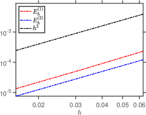
(a) $\theta=1/2$

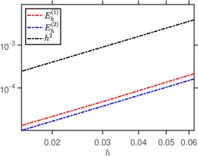
(b) $\theta=1$

Figure 4: The $\ell^{2}_{h,D}$-norms of the errors in the numerical approximation yielded by the first and second Laplacian, respectively, as functions of the spatial step size $h$, obtained using Algorithm 1 with (a) $\theta=1/2$ and (b) $\theta=1$, respectively, for $h\in\{1/16,1/32,1/64\}$.

Further, Figures 4 (a) and (b) display, on a logarithmic scale, the $\ell^{2}_{h,D}$ norms of the errors in the numerical approximation of the exact solution (8.3), i.e., $E^{(\ell)}_{h}$, $\ell=1,2$, corresponding to the first and second discrete Laplacian, respectively, obtained using Algorithm 1 with $\theta=\frac{1}{2}$ and $\theta=1$, respectively, as functions of the spatial grid size $h$, as well as the graph of the function $h^{2}$. It can be seen from this figure that the three graphs mentioned above are parallel, meaning that both numerical FDM discretisations of the Laplacian on ${\mathbb{H}^{2}}$ provide us with a numerical approximation for the exact solution with a sharp convergence rate of $\mathcal{O}(h^{2})$. Moreover, the comparison of the $\ell^{2}_{h,D}$-norms of the errors associated with the first and second discrete Laplace operators reveals that the latter numerical scheme yields a more accurate approximation. This result underscores the effectiveness of utilising a grid specifically adapted to the geometry of ${\mathbb{H}^{2}}$. Although not presented herein, similar results have been obtained when employing Algorithm 1 for various values for $\theta\in(1/2,1]$, confirming the sharp convergence rate of $\mathcal{O}(h^{2})$ for any choice of $\theta$.

8.3 Normalised relative error of the approximation

To investigate the precision of the pointwise approximation of the proposed algorithm, we define the normalised relative error in the numerically retrieved solution with respect to its analytical counterpart, namely

$$e^{(\ell)}_{h} \coloneqq\dfrac{\big{|}U^{(\ell)}_{h,i,j}-u^{(\mathrm{ex})}(T,\xi_{i,j})\big{|}}{\displaystyle\max_{\mathbf{y}\in{\mathbb{H}^{2}_{D}}}\big{|}u^{(\mathrm{ex})}(T,\mathbf{y})\big{|}},\quad(i,j)\in Z_{1}\times Z_{2}\,,\ell=\overline{1,2},\,\xi_{i,j}\text{ as in Lemma \ref{lem:approx-projection-with-pointwise}.}$$

32

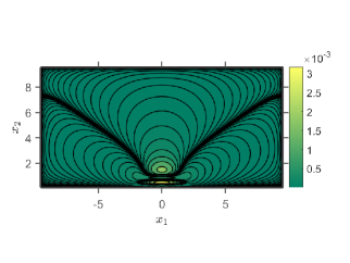
(a) $e^{(1)}_{h}$: First discrete Laplacian, $h=1/16$, $D=9.52$

(b) $e^{(2)}_{h}$ Second discrete Laplacian, $h=1/16$, $D=9.52$.

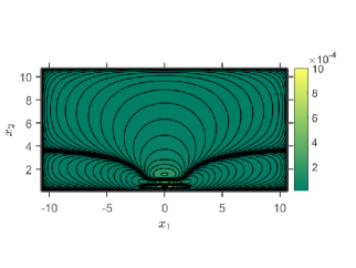
(c) $e^{(1)}_{h}$: First discrete Laplacian, $h=1/32$, $D=10.69$

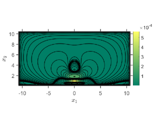
(d) $e^{(2)}_{h}$: Second discrete Laplacian, $h=1/32$, $D=10.69$

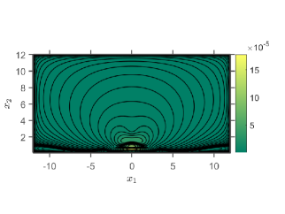
(e) $e^{(1)}_{h}$: First discrete Laplacian, $h=1/64$, $D=12$

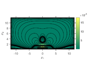
(f) $e^{(2)}_{h}$: Second discrete Laplacian, $h=1/64$, $D=12$

Figure 5: The normalised relative errors $e^{(1)}_{h}$, corresponding to the numerical approximation obtained using the first discrete Laplacian are displayed on the left-hand side above, whereas the error terms $e^{(2)}_{h}$, corresponding to the numerical approximation obtained using the second discrete Laplacian are on the right-hand side. The results were obtained using Algorithm 1 with $\theta=1/2$ and $h\in\{1/16,1/32,1/64\}$.

Figure 5 displays a comparison between the normalised relative errors obtained by employing the first discrete Laplacian in the $\theta$-scheme given by Algorithm 1 corresponding to $\theta=\frac{1}{2}$, illustrated in Figures 5 (a), (c) and (e), and their counterparts obtained via the second discrete Laplacian, depicted in Figures 5 (b), (d) and (f), for various spacial step sizes, $h\in\{1/16,1/32,1/64\}$. From this figures it can be seen that Algorithm 1 provides us with a numerical approximation convergent with respect to refining the finite difference grid for both discrete Laplacians considered, noting how the normalised relative errors $e^{(\ell)}_{h}$, $\ell=1,2$, decrease as $h$ decreases. Furthermore, by comparing Figures 5 (a) and (b) with Figures 5 (c) and (d), as well as with Figures 5 (e) and (f), it can be noted that the computational domain ${\mathbb{H}^{2}_{D}}$ increases as the stepsize $h$ decreases.

9 Conclusion and further research directions

9.1 Concluding remarks

In this paper, we have constructed two discrete finite-difference approximations of the Laplace-Beltrami operator on the 2-dimensional hyperbolic space ${\mathbb{H}^{2}}$, providing us with consistent, stable and thus convergent numerical schemes approximating the heat equation (1.3).

The consistency order of the aforementioned approximations has been proven to be $\mathcal{O}(h^{2})$, see Remarks 4.9 and 5.9, for the first and second discrete Laplacians, respectively. By employing a $\theta$-scheme to discretise the time variable, we propose Algorithm 1 to provide us with a numerical approximation of the solution of (1.3) with a convergence order of $\mathcal{O}(h^{2})$ for both discrete Laplacians, see Theorem 7.1.

The sharpness of this theoretical results is clearly illustrated by the numerical experiments conducted in Section 8, see Figure 4. Moreover, the suitability of the second discrete Laplace to the geometry of the hyperbolic space is emphasised from both a theoretical and a numerical point of view, see Remark 5.2 and, Tables 1–2, respectively.

It is worth noting that the numerical solution provided by Algorithm 1 is an approximation to its exact counterpart on the entire space ${\mathbb{H}^{2}}$. This has been achieved by defining the bounded domain ${\mathbb{H}^{2}_{D}}$ in terms of the mesh size, $h$, see (1.5), resulting in the enlargement of ${\mathbb{H}^{2}_{D}}$ with respect to the decrease of $h$, as it can be seen in Figure 5.

We also remark that, due to the consistency estimates in Sections 4 and 5, the results in this paper can be adapted in a classical way to the more straightforward cases of the stationary and the initial boundary value heat problems on bounded domains in ${\mathbb{H}^{2}}$.

9.2 Future work directions

We consider that this paper opens new research directions related to the problem of constructing a discrete counterpart to the Laplace-Beltrami operator on Riemannian manifolds. Some further research ideas related to the subject of this article are listed below in a synthetic manner.

1. Extend the analysis of FDM schemes for the heat equation to higher-dimensional hyperbolic spaces, $\mathbb{H}^{n}$, $n\geq 3$.

2. Produce other grids and corresponding discrete Laplacians better suited to the hyperbolic geometry, possibly using other models of the hyperbolic space. This is indeed a challenging problem, see Remark 5.1.

3. Study whether the discrete Laplace operator constructed in [9] using embedded graphs does fit into the framework of Sections 6 and 7, in terms of yielding a convergent numerical scheme.

4. Use the ideas in [37] to represent more accurately the numerical values of the grid functions in the computer’s memory and analyse whether there is a significant improvement in the accuracy of the approximation of (1.3) using the FDM schemes developed in the present paper.

5. Produce more accurate artificial conditions at the boundary of the bounded domian ${\mathbb{H}^{2}_{D}}$ using the explicit solution of the heat equation on ${\mathbb{H}^{2}}$, following the ideas in [30].

Appendix A Technical lemmata

A.1 Taylor estimates

For the sake of completion, we recall here some Taylor expansion formulas with integral reminder up to fourth order, for a real-valued function. They will be useful for proving the consistency estimates in this paper:

Lemma A.1.

Let $h,\varepsilon>0$ and $\varphi:(-h-\varepsilon,h+\varepsilon)\to\mathbb{R}$ a $C^{k}$ function, $k\in\{1,2,3,4\}$. Then, the following identities hold true:

1. For $k=1$,

   $$\varphi(h)=\varphi(0)+h\int_{0}^{1}\varphi^{\prime}(h\upsigma)\mathrm{d}\mathrm{\upsigma};$$

2. For $k=2$,

   $$\varphi(h)=\varphi(0)+h\varphi^{\prime}(0)+h^{2}\int_{0}^{1}\varphi^{\prime\prime}(h\upsigma)(1-\upsigma)\mathrm{d}\mathrm{\upsigma};$$

3. For $k=3$,

   $$\varphi(h)=\varphi(0)+h\varphi^{\prime}(0)+\frac{h^{2}}{2}\varphi^{\prime\prime}(0)+\frac{h^{3}}{2}\int_{0}^{1}\varphi^{\prime\prime\prime}(h\upsigma)(1-\upsigma)^{2}\mathrm{d}\mathrm{\upsigma};$$

4. For $k=3$, summing up iii) and the instance of iii) for $-h$, we get:

   $$\varphi(h)+\varphi(-h)-2\varphi(0)=h^{2}\varphi^{\prime\prime}(0)+\frac{h^{3}}{2}\int_{-1}^{1}\varphi^{\prime\prime\prime}(h\upsigma)(1-|\upsigma|)^{2}{\rm sgn}(\upsigma)\mathrm{d}\mathrm{\upsigma};$$

5. For $k=4$,

   $$\varphi(h)=\varphi(0)+h\varphi^{\prime}(0)+\frac{h^{2}}{2}\varphi^{\prime\prime}(0)+\frac{h^{3}}{6}\varphi^{\prime\prime\prime}(0)+\frac{h^{4}}{6}\int_{0}^{1}\varphi^{(4)}(h\upsigma)(1-\upsigma)^{3}\mathrm{d}\mathrm{\upsigma}.$$

6. For $k=4$, summing up v) and the instance of v) for $-h$, we get:

   $$\varphi(h)+\varphi(-h)-2\varphi(0)=h^{2}\varphi^{\prime\prime}(0)+\frac{h^{4}}{6}\int_{-1}^{1}\varphi^{(4)}(h\upsigma)(1-|\upsigma|)^{3}\mathrm{d}\mathrm{\upsigma};$$

7. For $k=4$, subtracting v) and the instance of v) for $-h$, we get:

   $$\varphi(h)-\varphi(-h)=2h\varphi^{\prime}(0)+\frac{h^{3}}{3}\varphi^{\prime\prime\prime}(0)+\frac{h^{4}}{6}\int_{-1}^{1}\varphi^{(4)}(h\upsigma)(1-|\upsigma|)^{3}{\rm sgn}(s)\mathrm{d}\mathrm{\upsigma};$$

Lemma A.2.

Let $\varphi:(e^{-h}-1-\varepsilon,e^{h}-1+\varepsilon)\to\mathbb{R}$ a $C^{4}$ function. Then,

$$\varphi(e^{h}-1)+e^{h}\varphi(e^{-h}-1)-(e^{h}+1)\varphi(0)= \frac{1}{2}(e^{h}-1)^{2}(1+e^{h})e^{-h}\varphi^{\prime\prime}(0)+\frac{1}{6}(e^{h}-1)^{4}(1+e^{h})e^{-2h}\varphi^{\prime\prime\prime}(0)$$

$$+\frac{1}{6}(e^{h}-1)^{4}e^{-3h/2}\int_{0}^{1}\sum_{\pm}e^{\pm 3h/2}\varphi^{(4)}((e^{\pm h}-1)\upsigma)(1-\upsigma)^{3}\mathrm{d}\mathrm{\upsigma};$$

Proof.

From Lemma A.1,

$$\varphi(e^{h}-1)=\varphi(0)+(e^{h}-1)\varphi^{\prime}(0)+\frac{(e^{h}-1){{}^{2}}}{2}\varphi^{\prime\prime}(0)+\frac{(e^{h}-1)^{3}}{6}\varphi^{\prime\prime\prime}(0)+\frac{(e^{h}-1)^{4}}{6}\int_{0}^{1}\varphi^{(4)}((e^{h}-1)\upsigma)(1-\upsigma)^{3}\mathrm{d}\mathrm{\upsigma};$$

Adding to the above Taylor expansion its instance for $-h$, multiplied by $e^{h}$, the conclusion follows. ∎

A.2 Proof of Lemma 4.4

Taking into account the zero average property of $\varphi$, one obtains that, for every $\mathbf{y}\in\Omega$,

$$I\coloneqq\int_{\Omega}v(\mathbf{x})\varphi(\mathbf{x})\mathrm{d}\mathrm{\mathbf{x}}=\int_{\Omega}(v(\mathbf{x})-v(\mathbf{y}))\varphi(\mathbf{x})\mathrm{d}\mathrm{\mathbf{x}}.$$

Integrating this relation with respect to $\mathbf{y}\in\Omega$, we recast $I$ as

$$I =\frac{1}{|\Omega|}\int_{\Omega}\int_{\Omega}(v(\mathbf{x})-v(\mathbf{y}))\varphi(\mathbf{x})\mathrm{d}\mathrm{\mathbf{x}}\mathrm{d}\mathrm{\mathbf{y}}=\frac{1}{|\Omega|}\int_{\Omega}\varphi(\mathbf{x})\int_{\Omega}\int_{0}^{1}\nabla_{e}v(\mathbf{x}+\upsigma(\mathbf{y}-\mathbf{x}))\cdot(\mathbf{x}-\mathbf{y})\mathrm{d}\mathrm{\upsigma}\mathrm{d}\mathrm{\mathbf{y}}\mathrm{d}\mathrm{\mathbf{x}}=$$

$$=\frac{1}{|\Omega|}\int_{\Omega}\varphi(\mathbf{x})\int_{\Omega}\int_{0}^{1}\nabla_{e}v(\mathbf{x}+\upsigma(\mathbf{y}-\mathbf{x}))\cdot(\mathbf{x}-\mathbf{y})\;\upchi_{\{\mathbf{x}+\upsigma(\mathbf{y}-\mathbf{x})\in\Omega\}}\,\mathrm{d}\mathrm{\upsigma}\,\mathrm{d}\mathrm{\mathbf{y}}\,\mathrm{d}\mathrm{\mathbf{x}},$$

where the last equality follows from the convexity of the domain $\Omega$. By employing the following change of variable $\mathbf{z}\coloneqq\mathbf{y}-\mathbf{x}$ and taking into account that $|\mathbf{x}-\mathbf{y}|\leq{\rm diam}(\Omega)$ we obtain:

$$|I| \leq\frac{1}{|\Omega|}\int_{\Omega}\varphi(\mathbf{x})\int_{0}^{1}\int_{B(0,{\rm diam}(\Omega))}\left|\nabla_{e}v(\mathbf{x}+\upsigma\mathbf{z})\cdot\mathbf{z}\right|\upchi_{\{x+\upsigma\mathbf{z}\in\Omega\}}\,\mathrm{d}\mathrm{\mathbf{z}}\,\mathrm{d}\mathrm{\upsigma}\,\mathrm{d}\mathrm{\mathbf{x}}$$

$$\leq\frac{{\rm diam}(\Omega)}{|\Omega|}\|\varphi\|_{\rm{L}^{\infty}(\Omega)}\int_{0}^{1}\int_{B(0,{\rm diam}(\Omega))}\int_{\Omega}\left|\nabla_{e}v(\mathbf{x}+\upsigma\mathbf{z})\right|\upchi_{\{x+\upsigma\mathbf{z}\in\Omega\}}\,\mathrm{d}\mathrm{\mathbf{x}}\,\mathrm{d}\mathrm{\mathbf{z}}\,\mathrm{d}\mathrm{\upsigma}.$$

Employing the change of variables $\omega\coloneqq\mathbf{x}+\upsigma\mathbf{z}$ in the inner integral, we obtain:

$$|I|\leq\frac{{\rm diam}(\Omega)}{|\Omega|}\|\varphi\|_{\rm{L}^{\infty}(\Omega)}\int_{0}^{1}\int_{B(0,{\rm diam}(\Omega))}\int_{\Omega}\left|\nabla_{e}v(\omega)\right|\,\mathrm{d}\mathrm{\omega}\,\mathrm{d}\mathrm{\mathbf{z}}\,\mathrm{d}\mathrm{\upsigma}=\pi\frac{\left({\rm diam}(\Omega)\right)^{3}}{|\Omega|}\|\varphi\|_{\rm{L}^{\infty}(\Omega)}\int_{\Omega}\left|\nabla_{e}v(\omega)\right|\,\mathrm{d}\mathrm{\omega}.$$

The conclusion follows by the Cauchy-Schwarz inequality. ∎

A.3 Sobolev inequality on Euclidean rectangles

Lemma A.3.

Let $\Omega=[y_{1},y_{1}+l_{1}]\times[y_{2},y_{2}+l_{2}]$ a non-degenerate rectangle in $\mathbb{R}^{2}$ with sides parallel with the axes. Then, there exists a universal constant $C>0$ such that, for any $v\in{\rm H}^{2}(\Omega)$,

$$\|v\|_{{\rm L}^{\infty}(\Omega)}\leq C\left|\Omega\right|_{e}^{-\frac{1}{2}}\max\left\{1,\left({\rm diam}_{e}(\Omega)\right)^{2}\right\}\|v\|_{{\rm H}^{2}(\Omega)}.$$

Proof.

Let $\Omega_{0}=[0,1]^{2}$ be the unit square. By the Sobolev Inequality [1, Theorem 4.12], there exists a constant $C$ such that, for $\tilde{v}\in{\rm H}^{2}(\Omega_{0})$,

$$\|\tilde{v}\|_{{\rm L}^{\infty}(\Omega_{0})}\leq C\|\tilde{v}\|_{{\rm H}^{2}(\Omega_{0})}.$$

Next, let $T$ be the affine transformation between $\Omega_{0}$ and $\Omega$:

$$T(x_{1},x_{2})=(y_{1}+x_{1}l_{1},y_{2}+x_{2}l_{2}).$$

Next, for an arbitrary $v\in{\rm H}^{2}(\Omega)$, we take $\tilde{v}=v\circ T\in{\rm H}^{2}(\Omega_{0})$. Since $\det(T)=l_{1}l_{2}=\left|\Omega\right|_{e}$, the change of variables formula leads to the following estimate:

$$\|\partial_{x_{1}}^{\alpha}\partial_{x_{2}}^{\beta}\tilde{v}\|_{{\rm L}^{2}(\Omega_{0})}=\left|\Omega\right|_{e}^{-\frac{1}{2}}l_{1}^{\alpha}l_{2}^{\beta}\|\partial_{x_{1}}^{\alpha}\partial_{x_{2}}^{\beta}v\|_{{\rm L}^{2}(\Omega)}\leq\left|\Omega\right|_{e}^{-\frac{1}{2}}\left({\rm diam}_{e}(\Omega)\right)^{\alpha+\beta}\|\partial_{x_{1}}^{\alpha}\partial_{x_{2}}^{\beta}v\|_{{\rm L}^{2}(\Omega)}.$$

As a result,

$$\|v\|_{{\rm L}^{\infty}(\Omega)}=\|\tilde{v}\|_{{\rm L}^{\infty}(\Omega_{0})}\leq C\|\tilde{v}\|_{{\rm H}^{2}(\Omega_{0})}\leq C\left|\Omega\right|_{e}^{-\frac{1}{2}}\max\left\{1,\left({\rm diam}_{e}(\Omega)\right),\left({\rm diam}_{e}(\Omega)\right)^{2}\right\}\|v\|_{{\rm H}^{2}(\Omega)}.$$

The conclusion follows. ∎

Appendix B Regularity and integrability of the solution of the heat equation on ${\mathbb{H}^{2}}$

Lemma B.1.

Let $D>2$ and $r_{D}\coloneqq\log(D/2)$. Let also $\mathrm{O}=(0,1)\in{\mathbb{H}^{2}}$. Then, the hyperbolic ball $B_{g}(\mathrm{O},r_{D})$ is contained inside the domain ${\mathbb{H}^{2}_{D}}=[-D,D]\times[1/D,D]$.

Proof.

We recall that the hyperbolic distance from the point $\mathrm{O}$ in the half-space model is given by:

$$d_{g}(\mathrm{O},\mathbf{x})=\mathrm{acosh}\left(1+\dfrac{x_{1}^{2}+(x_{2}-1)^{2}}{2x_{2}}\right).$$ (B.1)

Therefore, if $\mathbf{x}\in B(\mathrm{O},r_{D})$, then:

$$\dfrac{x_{1}^{2}+(x_{2}-1)^{2}}{2x_{2}}\leq\cosh(\log(D/2))-1=\frac{D}{4}+\frac{1}{D}-1.$$

Expanding the left-hand side term, we obtain:

$$\frac{x_{1}^{2}}{x_{2}}+x_{2}+\frac{1}{x_{2}}\leq\frac{D}{2}+\frac{2}{D},$$

from which we deduce that:

$$x_{2}\in\left[\frac{2}{D},\frac{D}{2}\right]\subset\left[\frac{1}{D},D\right]\hskip 5.69046pt\text{ and }\hskip 5.69046ptx_{1}^{2}\leq\frac{D^{2}}{4}+1\leq D^{2}.\qed$$

Lemma B.2.

Let $\alpha>0$, $\mathrm{O}=(0,1)\in{\mathbb{H}^{2}}$ and $u_{0}\in{\rm L}^{2}({\mathbb{H}^{2}})$. We denote by $e^{t\Delta_{g}}u_{0}$ the solution of the homogeneous heat equation on ${\mathbb{H}^{2}}$ (see (3.4)). Then, for every time $T>0$ there exists a constant $C_{\alpha,T}>0$ such that following inequality holds:

$$\left\|e^{\alpha d_{g}(\mathrm{O},\mathbf{x})}e^{t\Delta_{g}}u_{0}(\mathbf{x})\right\|_{{\rm L}^{2}({\mathbb{H}^{2}})}\leq C_{\alpha,T}\left\|e^{\alpha d_{g}(\mathrm{O},\mathbf{x})}u_{0}(\mathbf{x})\right\|_{{\rm L}^{2}({\mathbb{H}^{2}})},\,\forall t\in[0,T].$$

To prove the lemma, we recall the version of Young’s convolution inequality for integral kernels:

Proposition B.3 (Young’s inequality for integral kernels).

Let $(X,\mu_{X})$ and $(Y,\mu_{Y})$ be measure spaces and $\kappa:X\times Y\to\mathbb{R}$ a measurable kernel. If $p,q,r\geq 1$ satisfy

$$\frac{1}{r}+1=\frac{1}{p}+\frac{1}{q}$$

and there exists a constant $M>0$ such that $\kappa$ satisfies:

$$\int_{Y}|\kappa(\mathbf{x},\mathbf{y})|^{p}\mathrm{d}\mathrm{\mu_{Y}(\mathbf{y})}\leq M^{p},\forall\mathbf{x}\in X$$

and

$$\int_{X}|\kappa(\mathbf{x},\mathbf{y})|^{p}\mathrm{d}\mathrm{\mu_{X}(\mathbf{x})}\leq M^{p},\forall\mathbf{y}\in Y$$

then, for every measurable function $f:Y\to\mathbb{R}$,

$$\int_{X}\left|\int_{Y}\kappa(\mathbf{x},\mathbf{y})f(y)\mathrm{d}\mathrm{\mu_{Y}(\mathbf{y})}\right|^{r}\mathrm{d}\mathrm{\mu_{X}(\mathbf{x})}\leq M^{r}\left(\int_{Y}|f(y)|^{q}\mathrm{d}\mathrm{\mu_{Y}(\mathbf{y})}\right)^{\frac{r}{q}}.$$

Proof of Lemma B.2.

We recall that the solution of the homogeneous heat equation on ${\mathbb{H}^{2}}$ is given by the integral kernel representation (3.5), so the triangle inequality implies that:

$$e^{\alpha d_{g}(\mathrm{O},\mathbf{x})}e^{t\Delta_{g}}u_{0}(\mathbf{x})\leq\int_{{\mathbb{H}^{2}}}e^{\alpha d_{g}(\mathbf{x},\mathbf{y})}K(t,d_{g}(\mathbf{x},\mathbf{y}))e^{\alpha d_{g}(\mathrm{O},\mathbf{y})}u_{0}(\mathbf{y})\mathrm{d}\mathrm{\mu(\mathbf{y})}$$

Therefore, we apply Young’s inequality for $\kappa(x,y)=e^{\alpha d_{g}(\mathbf{x},\mathbf{y})}K(t,d(\mathbf{x},\mathbf{y}))$, $p=1$ and $q=r=2$. Since the kernel is non-negative and it only depends on the distance between $\mathbf{x}$ and $\mathbf{y}$, the quantity $M$ in Proposition B.3 is given as:

$$M\coloneqq\int_{{\mathbb{H}^{2}}}e^{\alpha d_{g}(\mathbf{x},\mathbf{y})}K(t,d(\mathbf{x},\mathbf{y}))\mathrm{d}\mathrm{\mu(\mathbf{y})},\,\forall\mathbf{x}\in{\mathbb{H}^{2}}.$$ (B.2)

We recall that the integration of radial functions on the hyperbolic space has the following form:

$$\int_{{\mathbb{H}^{2}}}f(d_{g}(x,y))dy=\int_{0}^{\infty}f(\uprho)\sinh(\uprho)\mathrm{d}\mathrm{\uprho},$$

so we rewrite (B.2) as:

$$M=\int_{0}^{\infty}e^{\alpha\uprho}K(t,\uprho)\sinh(\uprho)\mathrm{d}\mathrm{\uprho}.$$ (B.3)

We are left to show that $M$ can be bounded from above by a constant $C_{\alpha,T}$ depending only on $\alpha$ and $T$. Indeed, Proposition 3.6 implies that:

$$M\lesssim t^{-1}\int_{0}^{\infty}e^{-\frac{t}{4}-\frac{\uprho^{2}}{4t}+\left(\alpha-\frac{1}{2}\right)\uprho}\frac{1+\uprho}{\sqrt{1+\uprho+t}}\sinh(\uprho)\mathrm{d}\mathrm{\uprho},$$

which, by the change of variables $\uprho=s\sqrt{t}$ and taking into account that $\sinh(\uprho)\leq\uprho e^{\uprho}$ leads to:

$$M\lesssim \int_{0}^{\infty}e^{-\frac{t}{4}-\frac{s^{2}}{4}+\left(\alpha+\frac{1}{2}\right)s\sqrt{t}}\frac{s(1+s\sqrt{t})}{\sqrt{1+s\sqrt{t}+t}}\mathrm{d}\mathrm{s}$$

$$\leq\int_{0}^{\infty}e^{-\frac{t}{4}-\frac{s^{2}}{4}+\left(\alpha+\frac{1}{2}\right)s\sqrt{t}}s\sqrt{1+s\sqrt{t}}\,\mathrm{d}\mathrm{s}.$$

Since $\frac{s^{2}}{4}-\left(\alpha+\frac{1}{2}\right)s\sqrt{t}+\left(\alpha+\frac{1}{2}\right)^{2}t=\left(\frac{s}{2}-\left(\alpha+\frac{1}{2}\right)\sqrt{t}\right)^{2}$, we obtain:

$$M\lesssim e^{\alpha(\alpha+1)t}\int_{0}^{\infty}e^{-\left(\frac{s}{2}-\left(\alpha+\frac{1}{2}\right)\sqrt{t}\right)^{2}}s\sqrt{1+s\sqrt{t}}\,\mathrm{d}\mathrm{s}.$$

Changing the variables $\upsigma=\frac{s}{2}-\left(\alpha+\frac{1}{2}\right)\sqrt{t}$, we obtain:

$$M \lesssim e^{\alpha(\alpha+1)t}\int_{-\infty}^{\infty}e^{-\upsigma^{2}}\left[2\upsigma+2\left(\alpha+\frac{1}{2}\right)\sqrt{t}\right]\sqrt{1+\left[2\upsigma+2\left(\alpha+\frac{1}{2}\right)\sqrt{t}\right]\sqrt{t}}\,\mathrm{d}\mathrm{\upsigma}$$

$$\underbrace{\leq e^{\alpha(\alpha+1)T}\int_{-\infty}^{\infty}e^{-\upsigma^{2}}\left[2\upsigma+2\left(\alpha+\frac{1}{2}\right)\sqrt{T}\right]\sqrt{1+\left[2\upsigma+2\left(\alpha+\frac{1}{2}\right)\sqrt{T}\right]\sqrt{T}}\,\mathrm{d}\mathrm{\upsigma}}_{C_{\alpha,T}}.$$

The conclusion follows. ∎

Lemma B.4.

Let $D\coloneqq D_{h,\gamma,\zeta}$ chosen as in (1.6), $\alpha\in\{0,2\}$, $\beta\in\{2,4\}$. Then, there exists a constant $C_{\gamma,\zeta}>0$ such that, for any $v\in{\rm L}^{2}({\mathbb{H}^{2}})$ and any $h>0$,

$$\frac{D^{\alpha}}{h^{\beta}}\|v\|_{{\rm L}^{2}\left({\mathbb{H}^{2}}\setminus\mathbb{H}^{2}_{D}\right)}\leq C_{\gamma,\zeta}\left\|e^{\left(2+\frac{4}{\gamma}\right)d_{g}(\mathrm{O},\mathbf{x})}v(\mathbf{x})\right\|_{{\rm L}^{2}({\mathbb{H}^{2}})}.$$ (B.4)

Proof.

The particular choice of $D$ enables us to rewrite:

$$\frac{D^{\alpha}}{h^{\beta}}=\zeta^{-\frac{\beta}{\gamma}}D^{\alpha+\frac{\beta}{\gamma}}.$$

Further, Lemma B.1 implies that, if $\mathbf{x}\in{\mathbb{H}^{2}}\setminus\mathbb{H}^{2}_{D}$, then $d_{g}(\mathrm{O},\mathbf{x})\geq\log(D/2)$. In other words,

$$D\leq 2e^{d_{g}(\mathrm{O},\mathbf{x})},$$

so we can estimate the left-hand side term in (B.4) as follows:

$$\left(\frac{D^{\alpha}}{h^{\beta}}\right)^{2}\int_{{\mathbb{H}^{2}}\setminus\mathbb{H}^{2}_{D}}(v(\mathbf{x}))^{2}\mathrm{d}\mathrm{\mathbf{x}}\leq 2^{2\left(\alpha+\frac{\beta}{\gamma}\right)}\zeta^{-\frac{2\beta}{\gamma}}\int_{{\mathbb{H}^{2}}\setminus\mathbb{H}^{2}_{D}}e^{2\left(\alpha+\frac{\beta}{\gamma}\right)d_{g}(\mathrm{O},\mathbf{x})}(v(\mathbf{x}))^{2}\mathrm{d}\mathrm{\mathbf{x}}$$

and obtain the conclusion. ∎

B.1 Proof of Lemma 3.7

The first ingredient of the proof is the estimate for $\alpha=\beta=0$, with an extra term $|x_{1}|^{q}$, $q>0$:

$$\||x_{1}|^{q}x_{2}^{s}v(\mathbf{x})\|_{{\rm L}^{2}({\mathbb{H}^{2}})}\leq C_{q,s}\|e^{(q+|s|)d_{g}(\mathrm{O},\mathbf{x})}v(\mathbf{x})\|_{{\rm L}^{2}({\mathbb{H}^{2}})},\,v\in{\rm L}^{2}({\mathbb{H}^{2}})\,,$$ (B.5)

where we take, without losing generality, $\mathrm{O}=(0,1)\in{\mathbb{H}^{2}}$. To prove the above inequality, we use Lemma B.1 to deduce that, if $\mathbf{x}\in{\mathbb{H}^{2}}$ satisfies that $D_{\mathbf{x}}\coloneqq\max\{|x_{1}|,x_{2},\frac{1}{x_{2}}\}$ is greater than two, then, since $\mathbf{x}$ is on the boundary of $\mathbb{H}^{2}_{D_{\mathbf{x}}}$, it follows that $d_{g}(\mathrm{O},\mathbf{x})\geq\log(D_{\mathbf{x}}/2)$, which is equivalent to

$$|x_{1}|,x_{2},\frac{1}{x_{2}}\leq 2e^{d_{g}(\mathrm{O},\mathbf{x})}.$$ (B.6)

We note that if $D_{\mathbf{x}}\leq 2$, the inequality (B.6) is trivially true. The estimate (B.5) follows immediately from (B.6). Next, we apply it for $e^{t\Delta_{g}}u_{0}$ and use Lemma B.2 to obtain:

$$\||x_{1}|^{q}x_{2}^{s}e^{t\Delta_{g}}u_{0}\|_{{\rm L}^{2}({\mathbb{H}^{2}})}\leq C_{q,s,T}\|e^{(q+|s|)d_{g}(\mathrm{O},\mathbf{x})}u_{0}(\mathbf{x})\|_{{\rm L}^{2}({\mathbb{H}^{2}})},\,\forall u_{0}\in{\rm L}^{2}({\mathbb{H}^{2}}).$$ (B.7)

In the next step, we recall the form of the Laplace-Beltrami operator in the half-plane model of the $2$-dimensional hyperbolic space:

$$\Delta_{g}=x_{2}^{2}(\partial_{x_{1}}^{2}+\partial_{x_{2}}^{2}).$$ (B.8)

Since the left-hand side term of (3.8) contains the differential operator $\partial_{x_{1}}^{\alpha}\partial_{x_{2}}^{\beta}$ applied to the semigroup $(e^{t\Delta_{g}})_{t\geq 0}$ and we need to bound it by a similar expression at the initial time $t=0$ (i.e. an expression that depends only on $u_{0}$), we should, in some sense, commute the differential operator with the semigroup. This cannot be done directly, due to the extra term $x_{2}^{2}$ in the semigroup generator (B.8), so we will make use of several operators that do commute with $\Delta_{g}$ to obtain our desired result. These operators are:

$$\partial_{x_{1}} x_{1} {\mathbb{H}^{2}}$$ – corresponds to the translation in the direction, which is an isometry of ; (B.9)

$$x_{1}\partial_{x_{1}}+x_{2}\partial_{x_{2}} (0,0) {\mathbb{H}^{2}}$$ – corresponds to the Euclidean dilation centred in , which is an isometry of ; (B.10)

$$\Delta_{g}$$ – the Laplace-Beltrami operator itself. (B.11)

As a consequence,

$$\mathcal{T}u(t)=e^{t\Delta_{g}}\mathcal{T}u_{0},$$ (B.12)

where $\mathcal{T}$ is any of the operators above (or any combination – sums and compositions – of them). Our aim is to bound the operator $|\partial_{x_{1}}^{\alpha}\partial_{x_{2}}^{\beta}|$ form above with a combination (possibly weighted with powers of $x_{1}$ and $x_{2}$) of the aforementioned operators. Since $\partial_{x_{1}}$ commutes with $\Delta_{g}$, then we are left to process the term $\partial_{x_{2}}^{\beta}$. We will do this recursively depending on the order $\beta$ using the following identity, which is a direct consequence of (B.8):

$$\partial_{x_{2}}^{2}=x_{2}^{-2}\Delta_{g}-\partial_{x_{1}}^{2}.$$

Indeed, if $\beta\geq 2$, applying $\partial_{x_{2}}^{\beta-2}$ to the identity above implies:

$$\partial_{x_{2}}^{\beta}=\sum_{k=0}^{\beta-2}(-1)^{k}{\beta-2\choose k}(k+1)!\,x_{2}^{-2-k}\partial_{x_{2}}^{\beta-2-k}\Delta_{g}-\partial_{x_{2}}^{\beta-2}\partial_{x_{1}}^{2}.$$

Iterating this procedure, we arrive at:

$$\left|\partial_{x_{2}}^{\beta}\right|\leq C_{\beta}\sum_{\begin{subarray}{c}\sigma\in\{0,1\}\,\tau,\delta\in\mathbb{N}\\ \sigma+\tau+2\delta\leq\beta\\ k\in\overline{0,\beta}\end{subarray}}x_{2}^{-k}\left|\partial_{x_{2}}^{\sigma}\partial_{x_{1}}^{\tau}\Delta_{g}^{\delta}\right|.$$ (B.13)

If $\sigma=0$, we are done, since the operator $\partial_{x_{1}}^{\tau}\Delta_{g}^{\delta}$ commutes with $\Delta_{g}$. For the case $\sigma=1$, we make use of the operator (B.10) and write:

$$\partial_{x_{2}}=x_{2}^{-1}(x_{1}\partial_{x_{1}}+x_{2}\partial_{x_{2}})-x_{1}x_{2}^{-1}\partial_{x_{1}}.$$

Plugging this into (B.13), we obtain:

$$\left|\partial_{x_{2}}^{\beta}\right|\leq C_{\beta}\left\{\sum_{\begin{subarray}{c}k\in\overline{0,\beta},\,\tau,\delta\in\mathbb{N}\\ \tau+2\delta\leq\beta\end{subarray}}x_{2}^{-k}\left|\partial_{x_{1}}^{\tau}\Delta_{g}^{\delta}\right|+\sum_{\begin{subarray}{c}k\in\overline{0,\beta},\,\tau,\delta\in\mathbb{N}\\ 1+\tau+2\delta\leq\beta\end{subarray}}x_{2}^{-k-1}\left|(x_{1}\partial_{x_{1}}+x_{2}\partial_{x_{2}})\partial_{x_{1}}^{\tau}\Delta_{g}^{\delta}\right|+\sum_{\begin{subarray}{c}k\in\overline{0,\beta},\,\tau,\delta\in\mathbb{N}\\ 1+\tau+2\delta\leq\beta\end{subarray}}|x_{1}|x_{2}^{-k-1}\left|\partial_{x_{1}}^{\tau+1}\Delta_{g}^{\delta}\right|\right\}.$$ (B.14)

Further, we use (B.12) and (B.7) to obtain:

$$\sum_{\begin{subarray}{c}\alpha,\beta\in\mathbb{N}\\ \alpha+\beta\leq 6\end{subarray}}\|x_{2}^{s}\partial_{x_{1}}^{\alpha}\partial_{x_{2}}^{\beta}e^{t\Delta_{g}}u_{0}\|_{{\rm L}^{2}({\mathbb{H}^{2}})}\leq C_{s,T}\left\{\sum_{\begin{subarray}{c}k\in\overline{0,6},\,\tau,\delta\in\mathbb{N}\\ \tau+2\delta\leq 6\end{subarray}}\left\|e^{|s-k|d_{g}(\mathrm{O},\mathbf{x})}\partial_{x_{1}}^{\tau}\Delta_{g}^{\delta}u_{0}(\mathbf{x})\right\|_{{\rm L}^{2}({\mathbb{H}^{2}})}\right.$$ (B.15)

$$\left.+\sum_{\begin{subarray}{c}k\in\overline{0,6},\,\tau,\delta\in\mathbb{N}\\ 1+\tau+2\delta\leq 6\end{subarray}}\left\|e^{|s-k-1|d_{g}(\mathrm{O},\mathbf{x})}(x_{1}\partial_{x_{1}}+x_{2}\partial_{x_{2}})\partial_{x_{1}}^{\tau}\Delta_{g}^{\delta}u_{0}(\mathbf{x})\right\|_{{\rm L}^{2}({\mathbb{H}^{2}})}+\sum_{\begin{subarray}{c}k\in\overline{0,6},\,\tau,\delta\in\mathbb{N}\\ 1+\tau+2\delta\leq 6\end{subarray}}\left\|e^{(1+|s-k-1|)d_{g}(\mathrm{O},\mathbf{x})}\partial_{x_{1}}^{\tau+1}\Delta_{g}^{\delta}u_{0}(\mathbf{x})\right\|_{{\rm L}^{2}({\mathbb{H}^{2}})}\right\}$$

$$\leq C_{s,T}\left\{\sum_{\begin{subarray}{c}k\in\overline{0,6},\,\tau,\delta\in\mathbb{N}\\ \tau+2\delta\leq 6\end{subarray}}\left\|e^{(1+|s-k-1|)d_{g}(\mathrm{O},\mathbf{x})}\partial_{x_{1}}^{\tau}\Delta_{g}^{\delta}u_{0}(\mathbf{x})\right\|_{{\rm L}^{2}({\mathbb{H}^{2}})}+\sum_{\begin{subarray}{c}k\in\overline{0,6},\,\tau,\delta\in\mathbb{N}\\ 1+\tau+2\delta\leq 6\end{subarray}}\left\|e^{(1+|s-k-1|)d_{g}(\mathrm{O},\mathbf{x})}\partial_{x_{1}}^{\tau}\partial_{x_{2}}\Delta_{g}^{\delta}u_{0}(\mathbf{x})\right\|_{{\rm L}^{2}({\mathbb{H}^{2}})}\right\}.$$

In the end, taking into account the expression (B.8) for $\Delta_{g}$, we obtain that:

$$\left|\Delta_{g}^{\delta}\right|\leq\sum_{\begin{subarray}{c}k\in\overline{0,2\delta}\,\sigma,\tau\in\mathbb{N}\\ \sigma+\tau\leq 2\delta\end{subarray}}x_{2}^{k}\left|\partial_{x_{1}}^{\tau}\partial_{x_{2}}^{\sigma}\right|.$$ (B.16)

Together with (B.15) and (B.5), this inequality implies that:

$$\sum_{\begin{subarray}{c}\alpha,\beta\in\mathbb{N}\\ \alpha+\beta\leq 6\end{subarray}}\|x_{2}^{s}\partial_{x_{1}}^{\alpha}\partial_{x_{2}}^{\beta}e^{t\Delta_{g}}u_{0}\|_{{\rm L}^{2}({\mathbb{H}^{2}})}\leq C_{s,T}\sum_{\begin{subarray}{c}k\in\overline{0,6},\,\tau,\sigma\in\mathbb{N}\\ \tau+\sigma\leq 6\end{subarray}}\left\|e^{(7+|s-k-1|)d_{g}(\mathrm{O},\mathbf{x})}\partial_{x_{1}}^{\tau}\partial_{x_{2}}^{\sigma}u_{0}(\mathbf{x})\right\|_{{\rm L}^{2}({\mathbb{H}^{2}})}.$$

The conclusion follows by the triangle inequality in the exponential above.

Appendix C Proof of discrete Poincaré inequalities

C.1 Proof of Poincaré inequality for the first Laplacian (Proposition 4.3)

According to Proposition 4.2, we need to prove the following inequality:

$$\sum_{i\in\mathbb{Z},j\in\mathbb{N}}\left[(v_{i+1,j}-v_{i,j})^{2}+(v_{i,j+1}-v_{i,j})^{2}\right]\geq\frac{1}{4}\sum_{i\in\mathbb{Z},j\in\mathbb{N}}\frac{1}{j^{2}-1/4}|v_{i,j}|^{2},$$ (C.1)

with the convention $v_{i,0}=0$, $\forall i\in\mathbb{Z}$. Since the weights involved in the right-hand side term above only depend on the second variable (i.e. $j\in\mathbb{N}$), we consider first a single-variable sequence $(w_{j})_{j\in\mathbb{N}^{\ast}}$ and claim that:

$$\sum_{j\in\mathbb{N}}(w_{j+1}-w_{j})^{2}\geq\frac{1}{4}\sum_{j\in\mathbb{N}}\frac{1}{j^{2}-1/4}|w_{j}|^{2},$$ (C.2)

of course, employing the convention $w_{0}=0$. The proof of this claim is inspired by the study of a discrete Hardy inequality on the line [16]. Indeed, taking into account that $\sum_{j\geq 0}w_{j}^{2}=\sum_{j\geq 0}w_{j+1}^{2}$, we write the left-hand side term above as:

$$\sum_{j\in\mathbb{N}}(w_{j+1}-w_{j})^{2}=\sum_{j\in\mathbb{N}^{\ast}}\left(2-\sqrt{\frac{j-1}{j}}-\sqrt{\frac{j+1}{j}}\right)|w_{j}|^{2}+\sum_{j\in\mathbb{N}^{\ast}}\left(\sqrt[4]{\frac{j+1}{j}}w_{j}-\sqrt[4]{\frac{j}{j+1}}w_{j+1}\right)^{2}.$$ (C.3)

Therefore, in order to prove (C.2) it is sufficient to show that, for every $j\geq 1$,

$$2-\sqrt{\frac{j-1}{j}}-\sqrt{\frac{j+1}{j}}\geq\frac{1}{4(j^{2}-1/4)}.$$ (C.4)

Indeed, we transform the left-hand side of (C.4) and obtain:

$$2-\sqrt{\frac{j-1}{j}}-\sqrt{\frac{j+1}{j}} =\frac{\sqrt{j}-\sqrt{j-1}}{\sqrt{j}}-\frac{\sqrt{j+1}-\sqrt{j}}{\sqrt{j}}=\frac{1}{\sqrt{j}(\sqrt{j}+\sqrt{j-1})}-\frac{1}{\sqrt{j}(\sqrt{j+1}+\sqrt{j})}$$ (C.5)

$$=\frac{\sqrt{j+1}-\sqrt{j-1}}{\sqrt{j}(\sqrt{j}+\sqrt{j-1})(\sqrt{j+1}+\sqrt{j})}$$

$$=\frac{2}{\sqrt{j}(\sqrt{j}+\sqrt{j-1})(\sqrt{j+1}+\sqrt{j})(\sqrt{j+1}+\sqrt{j-1})}$$

The mean inequality implies that:

$$\sqrt{j}+\sqrt{j+1}\leq\sqrt{2(2j+1)}\text{ and }\sqrt{j}+\sqrt{j-1}\leq\sqrt{2(2j-1)},$$

therefore (C.5) leads to:

$$2-\sqrt{\frac{j-1}{j}}-\sqrt{\frac{j+1}{j}}\geq\frac{1}{2\sqrt{j^{2}-1/4}}\cdot\frac{1}{\sqrt{j}(\sqrt{j+1}+\sqrt{j-1})}.$$

We are now left to prove the following high-school level inequality:

$$\sqrt{j}(\sqrt{j+1}+\sqrt{j-1})\leq 2\sqrt{j^{2}-1/4},$$

which is left as an exercise to the reader. Therefore, the inequality (C.2) is proven. To obtain the desired inequality (C.1), all we need to do is to sum up the instances of (C.2) for every sequence $(v_{i,j})_{j\in\mathbb{N}^{\ast}}$ as $i\in\mathbb{Z}$.

To prove the sharpness of the constant $\frac{1}{4}$, first we will construct a minimizing sequence for the one-dimensional quantity:

$$\mathcal{I}(w):=\frac{\displaystyle\sum_{j\in\mathbb{N}}(w_{j+1}-w_{j})^{2}}{\displaystyle\sum_{j\in\mathbb{N}}\frac{1}{j^{2}-1/4}|w_{j}|^{2}}.$$ (C.6)

Since a minimizing sequence should annihilate the last term of (C.3), we will consider $w_{j}=\sqrt{j}$, but at the same time we properly cut it off in order to become compactly supported. More precisely, for every $n\in\mathbb{N}^{\ast}$, $n\geq 2$, we define (see [16, Section 2.2]):

$$w^{n}_{j}\coloneqq\sqrt{j}\cdot\left\{\begin{array}[]{cc}1,&1\leq j<n;\\ \frac{2\log n-\log j}{\log n},&n\leq j\leq n^{2};\\ 0,&j>n^{2}.\end{array}\right.$$ (C.7)

From (C.2) and (C.3) we obtain that:

$$0\leq I(w^{n})-\frac{1}{4}=\frac{\displaystyle\sum_{j\in\mathbb{N}^{\ast}}\left(\sqrt[4]{\frac{j+1}{j}}w^{n}_{j}-\sqrt[4]{\frac{j}{j+1}}w^{n}_{j+1}\right)^{2}+\sum_{j\in\mathbb{N}^{\ast}}\left(2-\sqrt{\frac{j-1}{j}}-\sqrt{\frac{j+1}{j}}-\frac{1}{4j^{2}-1}\right)|w_{j}^{n}|^{2}}{\displaystyle\sum_{j\in\mathbb{N}}\frac{1}{j^{2}-1/4}|w_{j}^{n}|^{2}}.$$ (C.8)

Next, we will analyse both sums at the numerator above:

$$\sum_{j\in\mathbb{N}^{\ast}}\left(\sqrt[4]{\frac{j+1}{j}}w^{n}_{j}-\sqrt[4]{\frac{j}{j+1}}w^{n}_{j+1}\right)^{2} =\sum_{j=n}^{n^{2}}\sqrt{j(j+1)}\left(\frac{\log(j+1)-\log(j)}{\log n}\right)^{2}=\sum_{j=n}^{n^{2}}\sqrt{j(j+1)}\left(\frac{\log\left(1+\frac{1}{j}\right)}{\log n}\right)^{2}$$

$$\leq\frac{1}{\log^{2}n}\sum_{j=n}^{n^{2}}\frac{\sqrt{j(j+1)}}{j^{2}}\lesssim\frac{1}{\log^{2}n}\sum_{j=n}^{n^{2}}\frac{1}{j}.$$

Then, standard properties of the harmonic series imply that:

$$\sum_{j\in\mathbb{N}^{\ast}}\left(\sqrt[4]{\frac{j+1}{j}}w^{n}_{j}-\sqrt[4]{\frac{j}{j+1}}w^{n}_{j+1}\right)^{2}\lesssim\frac{1}{\log n}.$$ (C.9)

Next, accounting to the second sum in the numerator of (C.8), we use (C.5) to write:

$$2-\sqrt{\frac{j-1}{j}}-\sqrt{\frac{j+1}{j}}-\frac{1}{4j^{2}-1}=\frac{8j^{2}-2-\sqrt{j}(\sqrt{j}+\sqrt{j-1})(\sqrt{j+1}+\sqrt{j})(\sqrt{j+1}+\sqrt{j-1})}{(4j^{2}-1)\sqrt{j}(\sqrt{j}+\sqrt{j-1})(\sqrt{j+1}+\sqrt{j})(\sqrt{j+1}+\sqrt{j-1})}.$$

Using that $\sqrt{j-1}<\sqrt{j}<\sqrt{j+1}$, we deduce that:

$$2-\sqrt{\frac{j-1}{j}}-\sqrt{\frac{j+1}{j}}-\frac{1}{4j^{2}-1}\leq\frac{8j^{2}-2-8j(j-1)}{8(4j^{2}-1)j(j-1)}=\frac{8j-2}{8(4j^{2}-1)j(j-1)}\lesssim\frac{1}{j^{3}}$$

By the construction (C.7) of the sequence $(w_{j}^{n})_{j\in\mathbb{N}^{\ast}}$, we have that:

$$\sum_{j\in\mathbb{N}^{\ast}}\left(2-\sqrt{\frac{j-1}{j}}-\sqrt{\frac{j+1}{j}}-\frac{1}{4j^{2}-1}\right)|w^{n}_{j}|^{2}\lesssim\sum_{j\geq 1}\frac{j}{j^{3}}=\frac{\pi^{2}}{6}.$$ (C.10)

Similarly, we can estimate the sum at the denominator of (C.8):

$$\sum_{j\in\mathbb{N}}\frac{1}{j^{2}-1/4}(w_{j}^{n})^{2}\gtrsim\sum_{j=1}^{n}\frac{1}{j}>\log n$$ (C.11)

Combining (C.8)-(C.11), we deduce that:

$$0\leq I(w^{n})-\frac{1}{4}\lesssim\frac{\frac{1}{\log n}+\frac{\pi^{2}}{6}}{\log n}\lesssim\frac{1}{\log n}\xrightarrow{n\to\infty}0,$$ (C.12)

which means that $(w^{n})_{n\geq 2}$ is a minimizing sequence for the functional $I$, thus proving the sharpness of the constant $\frac{1}{4}$ for the one-dimensional Poincaré-type inequality (C.2).

Based on the one-dimensional minimising sequence $(w^{n})_{n\geq 2}$, we now construct a minimizing double sequence $(v^{m,n})_{m,n\geq 2}$ for the functional:

$$\mathcal{J}(v):=\frac{\displaystyle\sum_{i\in\mathbb{Z},j\in\mathbb{N}}\left[(v_{i+1,j}-v_{i,j})^{2}+(v_{i,j+1}-v_{i,j})^{2}\right]}{\displaystyle\sum_{i\in\mathbb{Z},j\in\mathbb{N}}\frac{1}{j^{2}-1/4}v_{i,j}^{2}},$$ (C.13)

which, in turn, will prove the optimality of the constant $\frac{1}{4}$ in (C.1). Indeed, let us define $(v^{m,n}_{i,j})_{i\in\mathbb{Z},j\in\mathbb{N}^{\ast}}$ in the following way:

$$v^{m,n}_{i,j}\coloneqq\left\{\begin{array}[]{cc}w_{j}^{n}\left(1-\frac{|i|}{m}\right),&|i|\leq m\\ 0,&\text{otherwise}\end{array}\right.$$

The construction of $(v^{m,n}_{i,j})_{i\in\mathbb{Z},j\in\mathbb{N}^{\ast}}$, together with the inequality (C.1), implies that:

$$0\leq I(v^{m,n})-\frac{1}{4}=\frac{\displaystyle\left[\sum_{j\in\mathbb{N}}(w^{n}_{j+1}-w^{n}_{j})^{2}-\frac{1}{4}\sum_{j\in\mathbb{N}}\frac{1}{j^{2}-1/4}|w^{n}_{j}|^{2}\right]\sum_{|i|\leq m}\left(1-\frac{|i|}{m}\right)^{2}+\sum_{j\in\mathbb{N}}|w^{n}_{j}|^{2}\sum_{i=-m}^{m-1}\frac{1}{m^{2}}}{\displaystyle\sum_{j\in\mathbb{N}}\frac{1}{j^{2}-1/4}|w^{n}_{j}|^{2}\sum_{|i|\leq m}\left(1-\frac{|i|}{m}\right)^{2}}.$$

Making use of (C.12), we deduce that:

$$0\leq I(v^{m,n})-\frac{1}{4} \lesssim\frac{1}{\log n}+\frac{\displaystyle\sum_{j\in\mathbb{N}}|w^{n}_{j}|^{2}}{\displaystyle\sum_{j\in\mathbb{N}}\frac{1}{j^{2}-1/4}|w^{n}_{j}|^{2}}\cdot\frac{\displaystyle\sum_{i=-m}^{m-1}\frac{1}{m^{2}}}{\displaystyle\sum_{|i|\leq m}\left(1-\frac{|i|}{m}\right)^{2}}$$

$$\leq\frac{1}{\log n}+\frac{\displaystyle\sum_{j\in\mathbb{N}}|w^{n}_{j}|^{2}}{\displaystyle\sum_{j\in\mathbb{N}}\frac{1}{j^{2}-1/4}|w^{n}_{j}|^{2}}\cdot\frac{6}{2m^{2}+1}.$$

In the conclusion, for a fixed $\varepsilon>0$, we choose $n$ small enough such that $\frac{1}{\log n}\leq\frac{\varepsilon}{2}$ and then pass $m$ to infinity to get that the constant $\frac{1}{4}$ is sharp for (C.1).

C.2 Proof of Poincaré inequality for the second Laplacian

(Proposition 5.4)

First, we write the inequality that we aim to prove:

$$\sum_{i,j\in\mathbb{Z}}e^{jh}(v_{i+1,j}-v_{i,j})^{2}+\frac{2}{e^{h}+1}\sum_{i,j\in\mathbb{Z}}\frac{1}{e^{jh}}(v_{i,j+1}-v_{i,j})^{2}\geq C_{h}\,(\rho(h))^{2}\sum_{i,j\in\mathbb{Z}}\frac{1}{e^{jh}}|v_{i,j}|^{2}.$$ (C.14)

As in the case of the first Laplacian (Proposition 4.3), we prove a Poincaré-type inequality for an one-dimensional sequence $(w_{j})_{j\in\mathbb{Z}}$:

$$\frac{2}{e^{h}+1}\sum_{j\in\mathbb{Z}}\frac{1}{e^{jh}}(w_{j+1}-w_{j})^{2}\geq C_{h}\,(\rho(h))^{2}\sum_{j\in\mathbb{Z}}\frac{1}{e^{jh}}|w_{j}|^{2},$$ (C.15)

which, by direct computation, is equivalent to:

$$\sum_{j\in\mathbb{Z}}\frac{1}{e^{jh}}(w_{j+1}-w_{j})^{2}\geq(e^{h/2}-1)^{2}\sum_{j\in\mathbb{Z}}\frac{1}{e^{jh}}|w_{j}|^{2},$$ (C.16)

Indeed, this inequality is provd by noticing that the following identity holds:

$$\sum_{j\in\mathbb{Z}}\frac{1}{e^{jh}}(w_{j+1}-w_{j})^{2}=(e^{h/2}-1)^{2}\sum_{j\in\mathbb{Z}}\frac{1}{e^{jh}}w_{j}^{2}+\sum_{j\in\mathbb{Z}}\left(\frac{1}{e^{jh/2-h/4}}w_{j}-\frac{1}{e^{jh/2+h/4}}w_{j+1}\right)^{2}.$$ (C.17)

Eventually, to finish the proof of inequality (C.14), we sum the instances of (C.15) for $w_{j}=v_{i,j}$ over $i\in\mathbb{Z}$.

In the sequel, we prove the optimality of the constant $C_{h}$ for the Poincaré inequality (C.14). In this sense, we construct a family of compactly supported double sequences $(v^{m,n}_{i,j})_{i,j\in\mathbb{Z}}$ indexed over the integer parameters $m,n\geq 2$:

$$v^{m,n}_{i,j}=\left\{\begin{array}[]{cc}\left(1-\frac{|i|}{m}\right)e^{jh/2},&|i|\leq m\,,|j|\leq n;\\ 0,&\text{otherwise}.\end{array}\right.$$ (C.18)

We note that the part depending on $j$ (i.e. $e^{jh/2}$) was chosen as to annihilate the terms of the last sum in (C.17). We finish our proof by showing that the sequence constructed in (C.18) is a minimizing sequence for:

$$I(v)=\frac{\displaystyle\sum_{i,j\in\mathbb{Z}}e^{jh}(v_{i+1,j}-v_{i,j})^{2}+\frac{2}{e^{h}+1}\sum_{i,j\in\mathbb{Z}}\frac{1}{e^{jh}}(v_{i,j+1}-v_{i,j})^{2}}{\displaystyle\sum_{i,j\in\mathbb{Z}}\frac{1}{e^{jh}}v_{i,j}^{2}}.$$

Indeed, by direct computation,

$$I(v^{m,n}) =\frac{\displaystyle\sum_{i=-m}^{m-1}\frac{1}{m^{2}}\sum_{|j|\leq n}e^{2jh}+\frac{2}{e^{h}+1}\sum_{|i|\leq m}\left(1-\frac{|i|}{m}\right)^{2}\left[\sum_{j=-n}^{n-1}\frac{1}{e^{jh}}e^{jh}\left(e^{h/2}-1\right)^{2}+1+\frac{e^{-nh}}{e^{-(n+1)h}}\right]}{\displaystyle\sum_{|i|\leq m}\left(1-\frac{|i|}{m}\right)^{2}(2n+1)}$$

$$=\frac{\displaystyle\frac{2}{m}\sum_{|j|\leq n}e^{2jh}+\frac{2}{e^{h}+1}\frac{2m^{2}+1}{3m}\left[2n\left(e^{h/2}-1\right)^{2}+1+e^{h}\right]}{\displaystyle\frac{2m^{2}+1}{3m}(2n+1)}$$

$$=\frac{6}{2m^{2}+1}\frac{\displaystyle\sum_{|j|\leq n}e^{2jh}}{2n+1}+\frac{2}{e^{h}+1}\left[\frac{2n}{2n+1}\left(e^{h/2}-1\right)^{2}+\frac{1+e^{h}}{2n+1}\right]$$

Taking $n$ large enough and then $m\to\infty$, we obtain that the above quantity approaches:

$$\frac{2}{e^{h}+1}\left(e^{h/2}-1\right)^{2}=C_{h}(\rho(h))^{2}$$

and the conclusion follows.

References

- [1] Robert A. Adams and John J.. Fournier “Sobolev spaces” 140, Pure and Applied Mathematics (Amsterdam) Elsevier/Academic Press, Amsterdam, 2003, pp. xiv+305
- [2] F. Alvarez, J. Bolte and J. Munier “A unifying local convergence result for Newton’s method in Riemannian manifolds” In Found. Comput. Math. 8.2, 2008, pp. 197–226 DOI: 10.1007/s10208-006-0221-6
- [3] Paulo Amorim, Matania Ben-Artzi and Philippe G. LeFloch “Hyperbolic conservation laws on manifolds: total variation estimates and the finite volume method” In Methods Appl. Anal. 12.3, 2005, pp. 291–323 DOI: 10.4310/MAA.2005.v12.n3.a6
- [4] Jean-Philippe Anker, Effie Papageorgiou and Hong-Wei Zhang “Asymptotic behavior of solutions to the heat equation on noncompact symmetric spaces” In J. Funct. Anal. 284.6, 2023, pp. Paper No. 109828\bibrangessep43 DOI: 10.1016/j.jfa.2022.109828
- [5] Catherine Bandle, María del Mar González, Marco A. Fontelos and Noemi Wolanski “A nonlocal diffusion problem on manifolds” In Comm. Partial Differential Equations 43.4, 2018, pp. 652–676 DOI: 10.1080/03605302.2018.1459685
- [6] V. Banica “The nonlinear Schrödinger equation on hyperbolic space” In Comm. Partial Differential Equations 32.10-12, 2007, pp. 1643–1677 DOI: 10.1080/03605300600854332
- [7] John W. Barrett, Harald Garcke and Robert Nürnberg “Stable discretizations of elastic flow in Riemannian manifolds” In SIAM J. Numer. Anal. 57.4, 2019, pp. 1987–2018 DOI: 10.1137/18M1227111
- [8] Elvise Berchio, Debdip Ganguly, Gabriele Grillo and Yehuda Pinchover “An optimal improvement for the Hardy inequality on the hyperbolic space and related manifolds” In Proc. Roy. Soc. Edinburgh Sect. A 150.4, 2020, pp. 1699–1736 DOI: 10.1017/prm.2018.139
- [9] Dmitri Burago, Sergei Ivanov and Yaroslav Kurylev “A graph discretization of the Laplace-Beltrami operator” In J. Spectr. Theory 4.4, 2014, pp. 675–714 DOI: 10.4171/JST/83
- [10] T. Cazenave and A. Haraux “An Introduction to Semilinear Evolution Equations” Oxford University Press, 1998
- [11] A.. Cruzeiro and P. Malliavin “Numerical approximation of diffusions in using normal charts of a Riemaannian manifold” In Stochastic Process. Appl. 116.7, 2006, pp. 1088–1095 DOI: 10.1016/j.spa.2006.02.004
- [12] E.. Davies and N. Mandouvalos “Heat Kernel Bounds on Hyperbolic Space and Kleinian Groups” In Proceedings of the London Mathematical Society s3-57.1, 1988, pp. 182–208 DOI: https://doi.org/10.1112/plms/s3-57.1.182
- [13] Simone Fiori “Nonlinear damped oscillators on Riemannian manifolds: numerical simulation” In Commun. Nonlinear Sci. Numer. Simul. 47, 2017, pp. 207–222 DOI: 10.1016/j.cnsns.2016.11.025
- [14] Simone Fiori, Italo Cervigni, Mattia Ippoliti and Claudio Menotta “Synthetic nonlinear second-order oscillators on Riemannian manifolds and their numerical simulation” In Discrete Contin. Dyn. Syst. Ser. B 27.3, 2022, pp. 1227–1262 DOI: 10.3934/dcdsb.2021088
- [15] Harald Garcke and Robert Nürnberg “Numerical approximation of boundary value problems for curvature flow and elastic flow in Riemannian manifolds” In Numer. Math. 149.2, 2021, pp. 375–415 DOI: 10.1007/s00211-021-01231-6
- [16] Borbala Gerhat, David Krejcirik and Frantisek Stampach “An improved discrete Rellich inequality on the half-line”, 2022 arXiv:2206.11007 [math.SP]
- [17] Jan Giesselmann “A convergence result for finite volume schemes on Riemannian manifolds” In M2AN Math. Model. Numer. Anal. 43.5, 2009, pp. 929–955 DOI: 10.1051/m2an/2009013
- [18] María del Mar González, Liviu I. Ignat, Dragoş Manea and Sergiu Moroianu “Concentration limit for non-local dissipative convection–diffusion kernels on the hyperbolic space” In Nonlinear Anal. 248, 2024, pp. Paper No. 113618 DOI: 10.1016/j.na.2024.113618
- [19] Alexander Grigor’yan and Masakazu Noguchi “The Heat Kernel on Hyperbolic Space” In Bulletin of the London Mathematical Society 30.6, 1998, pp. 643–650 DOI: https://doi.org/10.1112/S0024609398004780
- [20] C. Grossman and H.-G. Roos “Numerical Treatment of Partial Differential Equations” Springer Berlin, Heidelberg, 2007
- [21] Sigurdur Helgason “Geometric analysis on symmetric spaces” 39, Mathematical Surveys and Monographs American Mathematical Society, Providence, RI, 2008, pp. xviii+637 DOI: 10.1090/surv/039
- [22] M. Holst “Adaptive numerical treatment of elliptic systems on manifolds” A posteriori error estimation and adaptive computational methods In Adv. Comput. Math. 15.1-4, 2001, pp. 139–191 DOI: 10.1023/A:1014246117321
- [23] B. Jovanović and E. Süli “Analysis of Finite Difference Schemes” Springer London, 2014
- [24] Alexandru Kristály “New features of the first eigenvalue on negatively curved spaces” In Adv. Calc. Var. 15.3, 2022, pp. 475–495 DOI: 10.1515/acv-2019-0103
- [25] Brice Loustau “Hyperbolic geometry”, 2020 arXiv: https://arxiv.org/abs/2003.11180v2
- [26] Francesco Mugelli and Giorgio Talenti “Sobolev inequalities in -D hyperbolic space: a borderline case” In J. Inequal. Appl. 2.3, 1998, pp. 195–228 DOI: 10.1155/S1025583498000125
- [27] Francesco Mugelli and Giorgio Talenti “Sobolev inequalities in -dimensional hyperbolic space” In General inequalities, 7 (Oberwolfach, 1995) 123, Internat. Ser. Numer. Math. Birkhäuser, Basel, 1997, pp. 201–216
- [28] Qu oc Anh Ngô and Van Hoang Nguyen “Sharp constant for Poincaré-type inequalities in the hyperbolic space” In Acta Math. Vietnam. 44.3, 2019, pp. 781–795 DOI: 10.1007/s40306-018-0269-9
- [29] Van Hoang Nguyen “The sharp Poincaré-Sobolev type inequalities in the hyperbolic spaces ” In J. Math. Anal. Appl. 462.2, 2018, pp. 1570–1584 DOI: 10.1016/j.jmaa.2018.02.054
- [30] Gang Pang, Yibo Yang and Shaoqiang Tang “Exact boundary condition for semi-discretized Schrödinger equation and heat equation in a rectangular domain” In J. Sci. Comput. 72.1, 2017, pp. 1–13 DOI: 10.1007/s10915-016-0344-0
- [31] Isaac Pesenson “A discrete Helgason-Fourier transform for Sobolev and Besov functions on noncompact symmetric spaces” In Radon transforms, geometry, and wavelets 464, Contemp. Math. Amer. Math. Soc., Providence, RI, 2008, pp. 231–247 DOI: 10.1090/conm/464/09087
- [32] Daniel Tataru “Strichartz estimates in the hyperbolic space and global existence for the semilinear wave equation” In Trans. Amer. Math. Soc. 353.2, 2001, pp. 795–807 DOI: 10.1090/S0002-9947-00-02750-1
- [33] R. Temam “On the Theory and Numerical Analysis of the Navier-Stokes Equations”, Lecture Note #9 University of Maryland, College Park, Maryland, 1973
- [34] Audrey Terras “Harmonic analysis on symmetric spaces—Euclidean space, the sphere, and the Poincaré upper half-plane” Springer, New York, 2013, pp. xviii+413 DOI: 10.1007/978-1-4614-7972-7
- [35] Juan Luis Vázquez “Asymptotic behaviour for the heat equation in hyperbolic space” In Comm. Anal. Geom. 30.9, 2022, pp. 2123–2156
- [36] Xiaonan Wu and Zhi-Zhong Sun “Convergence of difference scheme for heat equation in unbounded domains using artificial boundary conditions” In Appl. Numer. Math. 50.2, 2004, pp. 261–277 DOI: 10.1016/j.apnum.2004.01.001
- [37] Tao Yu and Christopher M De Sa “Numerically Accurate Hyperbolic Embeddings Using Tiling-Based Models” In Advances in Neural Information Processing Systems 32 Curran Associates, Inc., 2019 URL: https://proceedings.neurips.cc/paper_files/paper/2019/file/82c2559140b95ccda9c6ca4a8b981f1e-Paper.pdf
- [38] Chunxiong Zheng and Jiangming Xie “Fast artificial boundary method for the heat equation on unbounded domains with strip tails” In J. Comput. Appl. Math. 425, 2023, pp. Paper No. 115032\bibrangessep17 DOI: 10.1016/j.cam.2022.115032