Tripartite Entanglement In Mixed-Spin Triangle Trimer

Abstract

Heisenberg model spin systems offer favorable and manageable physical settings for generating and manipulating entangled quantum states. In this work mixed spin-(1/2,1/2,1) Heisenberg spin trimer with two different but isotropic Landé g-factors and two different exchange constants is considered. The study undertakes the task of finding the optimal parameters to create entangled states and control them by external magnetic field. The primary objective of this work is to examine the tripartite entanglement of a system and the dependence of the tripartite entanglement on various system parameters. Particularly, the effects of non-conserving magnetization are in the focus of our research. The source of non-commutativity between the magnetic moment operator and the Hamiltonian is the non-uniformity of g-factors. To quantify the tripartite entanglement, an entanglement measure called ”tripartite negativity” has been used in this work.

1 Introduction

Quantum entanglement, as a fundamental phenomenon in quantum mechanics, has attracted increasing attention recently due to its key role in quantum communication and information processing paradigms [1, 2, 3, 4, 5]. This non-classical correlation serves as a cornerstone for various quantum technologies, including quantum teleportation [6, 7, 8, 9, 10, 11], quantum computing [12, 13, 14], and quantum cryptography [15, 16]. Moreover, the study of entanglement has yielded significant insights in diverse fields, ranging from black hole physics, where it has facilitated progress in applying quantum field theory methods, to the investigation of quantum phase transitions and collective phenomena in many-body systems and condensed matter physics. In the last decades, significant research efforts have focused on investigating the entanglement properties of quantum spin clusters and molecular magnets [17, 18], motivated by compelling evidence suggesting that molecular magnets could serve as promising candidates for a physical realization of qubits in quantum information technologies [19, 20, 21]. This rapidly growing field has generated a substantial body of literature exploring various aspects of quantum entanglement in multi-body spin systems [22, 23, 24, 25, 26, 27, 28, 29, 30, 31, 32, 33, 34, 35, 36, 37, 38, 39, 40, 41], contributing to our understanding of quantum correlations at the molecular scale and their potential applications in quantum information science.

Magneto-thermal properties of single molecule magnets (SMM) are particularly sensitive to the situation when magnetic moment operator does not commute with the Hamiltonian, that gives rise to a non-conserving magnetization. The most common reason for the non-conserving magnetization is the different g-factors of different magnetic ions within the molecule [27, 29, 30, 42, 43, 44, 45, 46, 47, 48, 49, 50, 51, 52, 53]. Non-conserved magnetization can affect the magnetization curve drastically. When the magnetic moment is a good quantum number (conserving magnetization operator), then for the SMM, the magnetization curve at zero temperature consists of the series of horizontal parts (magnetization plateaus) with step-like transitions between them. Each plateau corresponds to certain eigenstate which is the ground state at given values of magnetic field. The constant value of the magnetic moment at each plateau is the expectation value of the magnetization operator for a given eigenstate. Transitions between plateaus correspond to level-crossing points. However, if the magnetization operator does not commute with the Hamiltonian, the magnetic field dependence within the given ground state can be continuous, as eigenstates with the given value of energy are not simultaneously eigenstates of the magnetic moment operator. Thus, even at zero temperature, the magnetization curve of SMM with non-conserving magnetization has much in common with magnetization curve of real many-body system [45, 46, 54]. Non-uniform $g$-factors can bring to drastic change of the eigenstates of finite spin cluster in comparison with the eigenstates of the same Hamiltonian but with uniform $g$-factors. These changes lead to incoherent superpositions of the spin states basic vectors with coefficients dependent on magnetic field magnitude and other parameters of the system. The latter, in its turn, opens new possibilities to manipulate quantum and/or thermal entanglement by means of magnetic field.

This study focuses on a mixed spin-($1/2,1/2,1$) trimer system with two distinct, yet isotropic, exchange interaction constants and non-conserved magnetization due to non-uniform $g$-factors. In our previous work we have examined properties of a bipartite entanglement for this system [40]. In this work we are going to investigate the tripartite entanglement of the system with the aid of the tripartite negativity measure. We analyze the dependence of negativity on various system parameters, including exchange interaction constants, non-conserved magnetization, and external magnetic field. A comparative analysis is conducted between the scenario involving non-conserved magnetization and the case with homogeneous $g$-factors. The investigation encompass several exchange interaction constants configurations:

A ferromagnetic interaction case ($J_{1}<0$, $J_{2}<0$), a scenario with two antiferromagnetic interactions $(J_{1}=J_{2}>0,J_{2}>J_{1}>0)$ and two mixed cases combining ferromagnetic and antiferromagnetic interactions($J_{1}>0,J_{2}<0$ and $J_{1}<0,J_{2}>0$)

The paper is organized as follows. In the Second section we introduce the quantum spin model and present its exact spectrum and eigenstates. The next Third section devoted to tripartite negativity. In the section IV we calculate tripartite negativity and present the plots of its magnetic field behaviour. The paper ends with Conclusion.

2 System

We consider a mixed spin trimer with spins 1/2, 1/2, and 1 in a triangular arrangement, with two different exchange couplings $J_{1}$ (between spin-1 and each spin-1/2) and $J_{2}$ (between spin-1/2 pairs) and two different g-factors, the one of 1/2 spins and the spin-1 ion have g-factor equal to $g_{1}$, while the other spin-1/2 ion has g-factor equal to $g_{2}$.

Figure 1: Symbolic picture of triangular trinuclear mixed-spin magnetic molecule with spins 1/2, 1/2 (small balls), and 1 (large ball). The Langè g-factors for one spin-1/2 ion and spin-1 ion are supposed to be the same ($g_{1}$), whereas the g-factor for the second spin-1/2 is different from them, $g_{2}$.

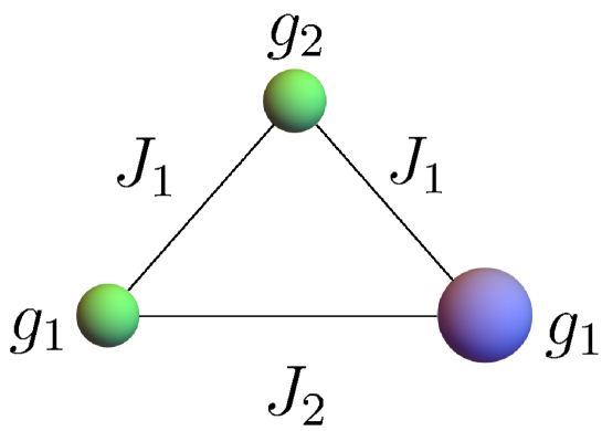
The spin Hamiltonian of the model has the following form:

$$\mathcal{H}=J_{1}\left(\boldsymbol{s}_{1}\boldsymbol{s}_{2}+\boldsymbol{s}_{2}\boldsymbol{S}_{3}\right)+J_{2}\boldsymbol{s}_{1}\boldsymbol{S}_{3}-B\left(g_{1}s_{1}^{z}+g_{2}s_{2}^{z}+g_{1}S_{3}^{z}\right)$$ (1)

where $\boldsymbol{s}_{a}$, $a=1,2$, are spin-1/2 operators, and $\boldsymbol{S}_{3}$ stands for spin-1 operators.

The eigenvalues and the eigenstates of the Hamiltonian are the followings [40]:

$${E}_{1,2} = \frac{1}{4}\left(3J_{1}+2J_{2}\mp 2B(3g_{1}+g_{2})\right),\>\>\>{E}_{3,4}=\frac{1}{4}\left(J_{1}-4J_{2}\mp 2B(g_{1}+g_{2})\right),$$ (2)

$${E}_{5,6} = \frac{1}{4}\left(-J_{1}-4J_{2}\mp 2\sqrt{B^{2}g_{-}^{2}+J_{1}^{2}}\right),\>\>\>{E}_{7,8}=\frac{1}{4}\left(-J_{1}+2J_{2}\mp 2\sqrt{B^{2}g_{-}^{2}+4J_{1}^{2}}\right),$$

$${E}_{9,10} = \frac{1}{4}\left(-J_{1}+2J_{2}-4Bg_{1}\mp 2Q^{+}\right),\>\>\>{E}_{11,12}=\frac{1}{4}\left(-J_{1}+2J_{2}+4Bg_{1}\mp 2Q^{-}\right),$$

$$\mbox{where}\;\;\;Q^{\pm} = \sqrt{(Bg_{-}\pm J_{1})^{2}+3J_{1}^{2}}.$$

$$|\psi_{1,2}\rangle=\left|\pm\frac{1}{2},\pm\frac{1}{2},\pm 1\right\rangle,$$ (3)

$$|\psi_{3,4}\rangle=\frac{1}{\sqrt{3}}\left(\pm\sqrt{2}\left|\mp\frac{1}{2},\pm\frac{1}{2},\pm 1\right\rangle\mp\left|\pm\frac{1}{2},\pm\frac{1}{2},0\right\rangle\right),$$

$$|\psi_{5,6}\rangle=\frac{1}{\sqrt{3(1+M^{2}_{\pm})}}\left(M^{\pm}\left(\sqrt{2}\left|\frac{1}{2},\frac{1}{2},-1\right\rangle-\left|-\frac{1}{2},\frac{1}{2},0\right\rangle\right)+\sqrt{2}\left|-\frac{1}{2},-\frac{1}{2},1\right\rangle-\left|\frac{1}{2},-\frac{1}{2},0\right\rangle\right),$$

$$|\psi_{7,8}\rangle=\frac{1}{\sqrt{3(4+K^{2}_{\mp})}}\left(K^{\mp}\left(\left|\frac{1}{2},\frac{1}{2},-1\right\rangle+\sqrt{2}\left|-\frac{1}{2},\frac{1}{2},0\right\rangle\right)+2\left|-\frac{1}{2},-\frac{1}{2},1\right\rangle+2\sqrt{2}\left|\frac{1}{2},-\frac{1}{2},0\right\rangle\right),$$

$$|\psi_{9,10}\rangle=\frac{1}{\sqrt{3+G^{2}_{\pm}}}\left(\sqrt{2}\left|\frac{1}{2},\frac{1}{2},0\right\rangle-G^{\pm}\left|\frac{1}{2},-\frac{1}{2},1\right\rangle+\left|-\frac{1}{2},\frac{1}{2},1\right\rangle\right),$$

$$|\psi_{11,12}\rangle=\frac{1}{\sqrt{3+U^{2}_{\mp}}}\left(\left|\frac{1}{2},-\frac{1}{2},-1\right\rangle+U^{\mp}\left|-\frac{1}{2},\frac{1}{2},-1\right\rangle+\sqrt{2}\left|-\frac{1}{2},-\frac{1}{2},0\right\rangle\right),$$

$$M^{\pm}=\frac{-Bg_{-}\pm\sqrt{B^{2}g_{-}^{2}+J_{1}^{2}}}{J_{1}},\quad K^{\pm}=\frac{Bg_{-}\pm\sqrt{B^{2}g_{-}^{2}+4J_{1}^{2}}}{2J_{1}},$$

$$G^{\pm}=\frac{Bg_{-}+J_{1}\pm Q^{+}}{J_{1}},\quad U^{\pm}=\frac{Bg_{-}-J_{1}\pm Q^{-}}{J_{1}},$$

As one of the main part of this research is devoted to the comparison of entanglement properties of the system with non-conserving magnetization and its uniform-$g$ counterpart, we have to use the corresponding eigenvectors for calculating the entanglement measures. However, the eigenvectors given above not always admit continuous limit at $g_{2}\rightarrow g_{1}$. For the case of uniform $g$-factors the corresponding Hamiltonian should be diagonalized separately. For the case $J_{1}=J_{2}$ and $g_{2}\rightarrow g_{1}$, the eigenvectors $|\psi_{3,4}\rangle$, $|\psi_{6}\rangle$, $|\psi_{7}\rangle$ $|\psi_{9}\rangle$ and $|\psi_{11}\rangle$ change non continuously. They acquire the following form:

$$|\psi_{3,4}\rangle_{0}=\frac{1}{2}\left(\left|\frac{1}{2},-\frac{1}{2},\pm 1\right\rangle+\left|-\frac{1}{2},\frac{1}{2},\pm 1\right\rangle-\sqrt{2}\left|\pm\frac{1}{2},\pm\frac{1}{2},0\right\rangle\right)$$ (4)

$$|\psi_{6}\rangle_{0}=\frac{1}{\sqrt{2}}\left(\left|-\frac{1}{2},-\frac{1}{2},1\right\rangle-\left|\frac{1}{2},\frac{1}{2},-1\right\rangle\right),\>\>\>|\psi_{7}\rangle_{0}=\frac{1}{\sqrt{2}}\left(\left|-\frac{1}{2},\frac{1}{2},0\right\rangle-\left|\frac{1}{2},-\frac{1}{2},0\right\rangle\right),$$

$$|\psi_{9}\rangle_{0}=\frac{1}{\sqrt{2}}\left(\left|-\frac{1}{2},\frac{1}{2},1\right\rangle-\left|\frac{1}{2},-\frac{1}{2},1\right\rangle\right),\>\>\>|\psi_{11}\rangle_{0}=\frac{1}{\sqrt{2}}\left(\left|-\frac{1}{2},\frac{1}{2},-1\right\rangle-\left|\frac{1}{2},-\frac{1}{2},-1\right\rangle\right).$$

The rest of the eigenvectors change continuously under $g_{2}\rightarrow g_{1}$. Detailed examination of system phase diagrams and magnetic properties was given in our previous work [40].

3 Tripartite Negativity

To quantifying the quantum entanglement several different entanglement measures can be used [1, 55]. However, for the mixed-spin clusters negativity [56] is the most convenient one, as it can be easily constructed and calculated for any pair of spins with the aid of reduced density matrix. For the system under consideration three pairwise bipartite negativities can be constructed. The numerical value on negativity, which varies from 0 (no entanglement) to $1/2$ (maximally entangled pair), corresponding to the i-th and j-th particles of the system, $Ne_{ij}$, equals to the sum of absolute values of negative eigenvalues of partially transposed reduced two-particle density matrix, $\rho_{ij}^{T}$, which is constructed in the following way:

$$\left\langle\tilde{\xi_{i}},\xi_{j}\right|\rho_{ij}^{T}\left|\xi_{i},\tilde{\xi_{j}}\right\rangle=\left\langle\xi_{i},\xi_{j}\left|\rho_{ij}\right|\tilde{\xi_{i}},\tilde{\xi_{j}}\right\rangle,$$ (5)

$$\rho_{ij}=\sum_{\xi_{k}}\left\langle\xi_{k}\left|\rho\right|\xi_{k}\right\rangle,\;\;k\neq i,j$$

where, $\left|\xi_{i},\xi_{j},\xi_{k}\right\rangle$ is a standard basis for the states of $\mathbf{s_{1}},\mathbf{s_{2}}$ ($\xi_{i}=\pm 1/2$) and $\mathbf{S_{3}}$ ($\xi_{i}=-1,0,1$) spins. Then the negativity is obtained according to

$$Ne_{ij}=\sum\limits_{a}|\mu_{a}|,$$ (6)

Bipartite negativity accounts for the entanglement between pairs of subsystems within the given system. In order to clarify the overall entanglement of three subsystems one can use the so-called, tripartite negativity [57]. In general in the system of three particles three different distributions of the entanglement can be found among its configurations : fully separable state, exhibiting no entanglement, three states where pair of particles are entangled, but the third particle is not (biseparable states) and one configuration in which all three particles are in the entangled state (tripartite entanglement) [57]. Tripartite negativity serves as an appropriate measure for characterizing the numerical degree of tripartite entanglement. This measure is defined by the following expression:

$$Ne_{ABC}=(Ne_{A-BC}Ne_{B-AC}Ne_{C-AB})^{1/3}$$ (7)

where $Ne_{A-BC},Ne_{B-AC},Ne_{C-AB}$ are generalized bipartite negativities between corresponding spin and the rest of the system. This quantity is calculated according to the similar formulas as given in Eqs. (5) - (6), when the trace in the Eq. (5) is not taken,

$$\left\langle\tilde{\xi_{i}},\xi_{j},\xi_{k}\right|\rho_{i-jk}^{T}\left|\xi_{i},\tilde{\xi_{j}},\tilde{\xi_{k}}\right\rangle=\left\langle\xi_{i},\xi_{j},\xi_{k}\left|\rho_{ijk}\right|\tilde{\xi_{i}},\tilde{\xi_{j}},\tilde{\xi_{k}}\right\rangle.$$ (8)

For mixed spin trimer(1/2, 1/2, 1) tripartite negativity can take values from 0 (no entanglement) to $\sqrt[3]{\frac{1}{4}}\approx 0.63$ (maximally entangled state). Here we deal only with purely quantum or zero-temperature entanglement, so the density matrix, $\rho$, we are working with is defined for each of the twelve eigenstates of the Hamiltonian as a pure-state density matrix:.

$$\rho_{i}=|\Psi_{i}\rangle\langle\Psi_{i}|,\;\;i=1,...,12.$$ (9)

In case of $n$ degenerate eigenstates one should use

$$\rho_{i_{1}...i_{n}}=\frac{1}{n}\sum_{a=1}^{n}|\Psi_{i_{a}}\rangle\langle\Psi_{i_{a}}|.$$ (10)

4 Results

According to the definition given above (Eq. (7)) we have obtained analytic expressions for the tripartite negativity for the eingenstates of the system under consideration. We present here only those which are relevant for the ground states phase diagram, obtained in our previous work [40]. As tripartite negativity is given by the Eq. (7) it is enough to know only all generalized bipartite negativities, $Ne^{i}_{A_{i}-A_{j}A_{k}}$. The index $i$ stands for the eigenstate numbering parameter. Bellow, we denote spin-1/2 ion with $g$-factor equal to $g_{1}$ by $A$, spin-1/2 ion with $g$-factor equal to $g_{2}$ by $B$ and ion with spin-1 by $C$. Interestingly, some eigenstates can have the same $Ne^{i}_{A_{i}-A_{j}A_{k}}$.

$$Ne^{3,4}_{A-BC}=Ne^{3,4}_{C-AB}=\frac{\sqrt{2}}{3},\>\>\>\>\>\>Ne^{3,4}_{B-AC}=0,\>\>\>\>\>\>Ne^{5,6}_{A-BC}=\frac{\sqrt{2M_{\pm}^{4}+5M_{\pm}^{2}+2}}{3\left(M_{\pm}^{2}+1\right)},$$ (11)

$$Ne^{5,6}_{B-AC}=\left|\frac{M_{\pm}}{M_{\pm}^{2}+1}\right|,\>\>\>\>\>\>Ne^{5,6}_{C-AB}=\frac{2}{3}\left|\frac{M_{\pm}}{M_{\pm}^{2}+1}\right|+\frac{\sqrt{2}\sqrt{M_{\pm}^{4}+M_{\pm}^{2}}}{3\left(M_{\pm}^{2}+1\right)}+\frac{\sqrt{2}}{3\sqrt{M_{\pm}^{2}+1}},$$

$$Ne^{7,8}_{A-BC}=\frac{\sqrt{2}\sqrt{K_{\mp}^{4}+10K_{\mp}^{2}+16}}{3\left(K_{\mp}^{2}+4\right)},\>\>\>\>\>\>Ne^{7,8}_{B-AC}=2\left|\frac{K_{\mp}}{K_{\mp}^{2}+4}\right|,$$

$$Ne^{7,8}_{C-AB}=\frac{2}{3}\left|\frac{K_{\mp}}{K_{\mp}^{2}+4}\right|+\frac{\sqrt{2}\sqrt{K_{\mp}^{4}+4K_{\mp}^{2}}}{3\left(K_{\mp}^{2}+4\right)}+\frac{2\sqrt{2}}{3\sqrt{K_{\mp}^{2}+4}},\>\>\>\>\>\>Ne^{9,10}_{A-BC}=\frac{\sqrt{G_{\pm}^{2}+2}}{G_{\pm}^{2}+3},$$

$$Ne^{9,10}_{B-AC}=\sqrt{3}\left|\frac{G_{\pm}}{G_{\pm}^{2}+3}\right|,\>\>\>\>\>\>Ne^{9,10}_{C-AB}=\frac{\sqrt{2}\sqrt{G_{\pm}^{2}+1}}{G_{\pm}^{2}+3},\>\>\>\>\>\>Ne^{11,12}_{A-BC}=\sqrt{3}\left|\frac{U_{\mp}}{U_{\mp}^{2}+3}\right|,$$

$$Ne^{11,12}_{B-AC}=\frac{\sqrt{U_{\mp}^{2}+2}}{U_{\mp}^{2}+3},\>\>\>\>\>\>Ne^{11}_{C-AB}=\frac{\sqrt{2}\sqrt{U_{\mp}^{2}+1}}{U_{\mp}^{2}+3}.$$

In our previous work a detailed analysis of the ground states phase diagrams of the system were presented [40]. Here we demonstrate only those of them, which exhibit interesting features of the tripartite negativity dependent on the value on non-uniform $g$-factor. The main purpose of the present research is to figure out how non-uniform $g$-factors affect tripartite entanglement properties of the model. It is worth mentioning, that the most remarkable enhancement of the bipartite negativity caused by non-uniform $g$-factors reported in our previous work [40] concerned the case $J_{2}=J_{1}$ and gave almost 7-fold robust decrease of $Ne_{12}$ for arbitrary small difference between $g_{2}$ and $g_{1}$. For the tripartite entanglement situation is quite different. Here we presented density plots of the tripartite negativity, $Ne_{ABC}$, projected onto ground state phase diagrams in the ”$g$-factors ration” - ”dimensionless magnetic field” plane.

Figure 2: Density plots of tripartite negativity for $J_{1}=J_{2}>0$ (panel a), $J_{2}>0\,\,\text{and}\,\,J_{1}=\frac{1}{5}J_{2}$ (panel b) and $J_{2}>0\,\,\text{and}\,\,J_{1}=-\frac{1}{5}J_{2}$ (panel c) cases.

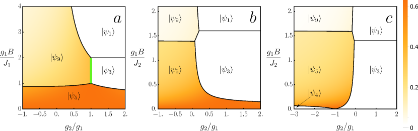
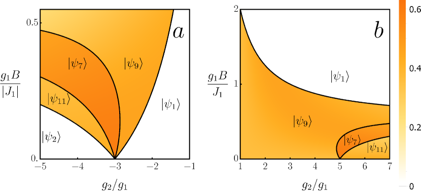
Two antiferromagnetic cases, $J_{1}=J_{2}>0$, $J_{2}>0\,\,\text{and}\,\,J_{1}=\frac{1}{5}J_{2}$, and a mixed case, $J_{2}>0\,\,\text{and}\,\,J_{1}=-\frac{1}{5}J_{2}$, are presented in the Fig. 2. In the case of equal antiferromagnetic coupling (panel a) the phase diagram includes four eigenstates $|\psi_{1}\rangle,|\psi_{3}\rangle,|\psi_{5}\rangle$ and $|\psi_{9}\rangle$. However, two of them $|\psi_{3}\rangle$ and $|\psi_{9}\rangle$ transform non-continuously under $g_{2}\rightarrow g_{1}$. For uniform situation, $g_{2}=g_{1}$, degeneracy line between $|\psi_{3}\rangle$ and $|\psi_{9}\rangle$ regions corresponds to the degenerate superposition of $|\psi_{3}\rangle_{0}$ and $|\psi_{9}\rangle_{0}$ given in the Eq. (4). This segment is highlighted in green in the right panel on the Fig. 2. The value of the tripartite negativity here is $Ne_{ABC}^{(3+9)_{0}}=\frac{1}{2}\sqrt[3]{\frac{3}{4}}\approx 0.45$. Interestingly, the $|\psi_{5}\rangle$ eigenstate, which is the zero-field ground state for arbitrary value of $g_{2}/g_{1}$, exhibits maximal three-particle entanglement at $B=0$ and at the segment $g_{2}=g_{1}$, $Ne_{ABC}^{5}=\sqrt[3]{\frac{1}{4}}\approx 0.63$. The most dramatic discrepancy between bipartite and tripartite entanglement properties is occurred for the $|\psi_{3}\rangle$ eigenstate, for which one of the bipartite negativities becomes almost seven times larger than the corresponding uniform-$g$ value [40]. Tripartite negativity is zero for $|\psi_{3}\rangle$, which means that this state is biseparable. Thus, in the case of $g_{2}>g_{1}$, when magnetization is not conserved, it is possible to create two significantly different entanglement regimes and control them by external magnetic field. First regime exhibits maximum value for tripartite entanglement, when the second regime exhibits maximum value for bipartite entanglement and have no tripartite entanglement. As usual, for the large enough magnetic field the system reaches its saturated ($|\psi_{1}\rangle$) or quasi-saturates ($|\psi_{9}\rangle$) states with zero or vanishing entanglement. For the case $J_{2}>0,\,\,J_{1}=\frac{1}{5}J_{2}$ (Fig. 2, panel b) system exhibits similar behavior, there are eigenstates with strong bipartite entanglement, but with zero $Ne_{ABC}$, $|\psi_{3}\rangle$ and region where both quantities are quite large, $|\psi_{5}\rangle$. However, presence of non-conserving magnetization does not bring any quantitative or qualitative benefits. The only difference between $g_{2}=g_{1}$ and $g_{2}\neq g_{1}$ cases are that for the second case tripartite negativity is depended on magnetic field within the same ground state. Fig. 2 (panel c) shows density plot of tripartite negativity for the $J_{2}>0,\,\,J_{1}=-\frac{1}{5}J_{2}$ case. Here system have one additional region of ground state corresponding to $|\psi_{4}\rangle$. Here in contrast to the previous cases, regime with maximal or essentially large $Ne_{ABC}$ is absent. System exhibits maximal entanglement under the conditions $g_{2}=-g_{1}$ and when magnetic field is close to zero. In the Fig. 3 the cases $J_{1}<0$, arbitrary $J_{2}\leq 0$ and $J_{1}>0$, arbitrary $J_{2}<0$ are presented. For both cases maximal possible tripartite negativity achieved for the eigenstate $|\psi_{7}\rangle$ with value 0.59.

Figure 3: Density plots of tripartite negativity for $J_{1}<0$, arbitrary $J_{2}\leq 0$ and $J_{1}>0$, arbitrary $J_{2}<0$ cases in panels a and b respectfully.

5 Conclusion

In the paper we considered the mixed spin (1/2, 1/2, 1) Heisenberg spin trimer with non-conserving magnetization. Analytical results for tripartite negativity were obtained for all ground states. In general, depending on the relations between two exchange constants, the system can exhibit five regimes of magnetic behavior [40]. These regimes, in their turn, are storngly affected by the ration of the $g$-factors, $g_{2}/g_{1}$. It was shown that in fully antiferromagnetic cases, it is possible to obtain a three-regime system (fully separable, biseparable, tripartite entangled) and control it by magnetic field. In the case $J_{2}=J_{1}>0$ these regimes are possible only when $g_{2}>g_{1}$, when magnetisation is not-conserving.

6 Acknowledgements

The authors acknowledge partial financial support form ANSEF (Grants No. PS-condmatth-2462 and PS-condmatth-2884) and from CS RA MESCS (Grants No. 21AG-1C047, 21AG-1C006 and 23AA-1C032).

References

- [1] Amico L, Fazio R, Osterloh A and Vedral V 2008 Rev. Mod. Phys. 80 517
- [2] Gühne O and Tóth G 2009 Phys. Rep. 474 1
- [3] Bennett C H, DiVincenzo D P, Smolin J A and Wootters W K 1996 Phys. Rev. A 54 3824
- [4] Bennett C H, Brassard G, Popescu S, Schumacher B, Smolin J A and Wootters W K 1996 Phys. Rev. Lett 76 722
- [5] Ekert A K 1992 Nature (London) 358 14
- [6] Bennett C H, Brassard G, Crépeau C, Jozsa R, Peres A and Wootters W K 1993 Phys. Rev. Lett. 70 1895
- [7] Bouwmeester D, Pan J W, Mattle K, Eibl M, Weinfurter H and Zeilinger A 1997 Nature (London) 390 575
- [8] Cho J and Lee H-W 2005 Phys. Rev. Lett. 95 160501
- [9] Jin X-M, Ren J-G, Yang B, Yi Z-H, Zhou F, Xu X-F, Wang S-K, Yang D, Hu Y-F, Jiang S, Yang T, Yin H, Chen K, Peng C-Z and Pan J-W 2010 Nature Photonics 4 376
- [10] Baur M, Fedorov A, Steffen L, Filipp S, da Silva M P and Wallraff A 2012 Phys. Rev. Lett. 108 040502
- [11] Björk G, Laghaout A and Andersen U L2012 Phys. Rev. A 85 022316
- [12] Kok P, Munro W J, Nemoto K, Ralph T C, Dowling J P and Milburn G J 2007 Rev. Mod. Phys. 79 135
- [13] Kim J, Lee J-S, Lee S and Cheong C 2000 Phys. Rev. A 62 022312
- [14] Brodutch A and Terno D R 2011 Phys. Rev. A 83 010301(R)
- [15] Vedral V and Kashefi E 2002 Phys. Rev. Lett. 89, 037903
- [16] Avella A, Brida G, Degiovanni I P, Genovese M, Gramegna M and Traina P 2010 Phys. Rev. A 82 062309
- [17] Coronado E 2020 Nature Rev. Mat. 5 87
- [18] Kahn O 1993 Molecular Magnetism (New York: Wiley)
- [19] Leuenberger M N and Loss D 2001 Nature 410 789
- [20] Stepanenko D, Trif M and Loss D 2008 Inorganica Chimica Acta 361 3740
- [21] Sessoli R 2015 ACS Cent. Sci. 1 473
- [22] Ananikian N S, Ananikyan L N, Chakhmakhchyan L A and Kocharian A N 2011 J. Phys.: Math. Theor. 44 025001
- [23] Abgaryan V S, Ananikian N S, Ananikyan L N and Kocharian A N 2011 Phys. Ser. 83 055702
- [24] Ananikian N, Lazaryan H and Nalbandyan M 2012Eur. Phys. J. B 85 223
- [25] Strečka J, Rojas O, Verkholyak T and Lyra M L 2014 Phys. Rev. E 89 022143
- [26] Carvalho I M, Torrico J, de Souza S M, Rojas M and Rojas O 2018 J. Mag. Magn. Mater. 465 323
- [27] Souza F, Lyra M L, Strečka J and Pereira M S S 2019 J. Mag. Magn. Mater. 471 423
- [28] Souza F, Veríssimo L M, Strečka J, Lyra M L and Pereira M S S 2020 Phys. Rev. B 102 064414
- [29] Adamyan Zh, Muradyan S and Ohanyan V 2020 J. Contemp. Phys. 55 292
- [30] Čenčarikova H and Strečka J 2020 Phys. Rev. B 102 184419
- [31] Ekiz C and Strečka J 2020 Acta Phys. Pol. A 137 592
- [32] Karĺová K and Strečka J 2020 Acta Phys. Pol. A 137, 595
- [33] Strečka J, Krupnitska O and Richter J 2020 EPL 132 30004
- [34] Gálisová L, Strečka J, Verkholyak T and Havadej S 2021 Physica E 125 114089
- [35] Gálisová L and Kaczor M, 2021 Entropy 23 1671
- [36] Gálisová L 2022 J. Magn. Magn. Mater. 561 169721
- [37] Benabdallah F, Haddadi S, Arian Zad H, Pourkarimi M R, Daoud M and Ananikian N 2022 Sci. Rep. 12 6406
- [38] Arian Zad H, Zoshki A, Ananikian N and Jaščur M 2022 J. Mag. Magn. Mater. 559 169533
- [39] Zheng Y-D and Zhou B 2022 Physica A 603 127753
- [40] Adamyan Zh and Ohanyan V 2024 Phys. Rev. E submitted (arxiv.org/abs/2405.00178)
- [41] Ghannadan A, Arian Zad H, Haddadi S, Strečka J, Adamyan Zh, and Ohanyan V, Phys. Rev. A submitted (arXiv.org/abs/2407.07037).
- [42] Strečka J, Jaščur M, Hagiwara M, Minami K, Narumi Y and Kindo K, 2005 Phys. Rev. B 72 024459
- [43] Visinescu D, Madalan A M, Andruh M, Duhayon C, Sutter J-P, Ungur L, Van den Heuvel W and Chibotaru L F 2009 Chem. Eur. J. 15 11808
- [44] Van den Heuvel W and Chibotaru L F 2010 Phys. Rev. B 82 174436
- [45] Bellucci S, Ohanyan V and Rojas O 2014 EPL 105 47012
- [46] Ohanyan V, Rojas O, Strečka J and Bellucci S 2015 Phys. Rev. B 92 184427
- [47] Torrico J, Rojas M, de Souza S M and Rojas O 2016 Phys. Lett. 380 3655
- [48] Torrico J, Ohanyan V and Rojas O 2018 J. Magn. Magn. Mater 454 85
- [49] Varizi A D and Drumond R C 2019 Phys. Rev. E 100 022104
- [50] Krokhmalskii T, Verkholyak T, Baran O, Ohanyan V and Derzhko O, 2020 Phys. Rev. B 102 144403
- [51] Pandey T and Chitov G Y 2020 Phys. Rev. B 102 054436
- [52] Japaridze G I, Cheraghi H and Mahdavifar S, 2021 Phys. Rev, E 104 014131
- [53] Baran O R, 2023 Ukr. J. Phys. 68 488
- [54] Vargovà H and Strečka J, 2022 Eur. Phys. J. Plus 137 490
- [55] Horodecki R, Horodecki P, Horodecki M and Horodecki K 2009 Rev. Mod. Phys. 81 865
- [56] Vidal G and Werner R W 2002 Phys. Rev. A, 65 032314
- [57] Sabín C and García-Alcaine G 2008 Eur. Phys. J. D 48 435–442