A Hybrid Algorithm for Systems of Non-interacting Particles

Abstract

Our focus is on simulating the dynamics of non-interacting particles, which, under certain assumptions, can be formally described by the Dean-Kawasaki equation. The Dean-Kawasaki equation can be solved numerically using standard finite volume methods. However, the numerical approximation implicitly requires a sufficiently large number of particles to ensure the positivity of the solution and accurate approximation of the stochastic flux. To address this challenge, we extend hybrid algorithms for particle systems to scenarios where the density is low. The aim is to create a hybrid algorithm that switches from a finite volume discretization to a particle-based method when the particle density falls below a certain threshold. We develop criteria for determining this threshold by comparing higher-order statistics obtained from the finite volume method with particle simulations. We then demonstrate the use of the resulting criteria for dynamic adaptation in both two- and three-dimensional spatial settings.

1 Introduction

The dynamics of a system of non-interacting random-walker particles can, in a suitable mathematical setting, be formally described by the Dean-Kawasaki equation. The microscopic model that we are considering is a random walk of $N$ independent indistinguishable Brownian particles $\{B_{t}^{i}\}_{i=1}^{N}$ on a $d$-dimensional torus $\mathbb{T}^{d},d\in\{1,2,3\}$ or with Dirichlet or homogeneous Neumann boundary conditions on a rectilinear domain. Let $\mu^{N}_{t}$ be the empirical density that is defined by

$$\mu_{t}^{N}(x,t):=\frac{1}{N}\sum_{i=1}^{N}\delta_{B_{t}^{i}}(x),$$ (1)

where $\delta$ is a Dirac distribution. Utilizing the Itô’s formula one can formally derive the equation for $\mu^{N}$, see [10, 19]. The formal form of the equation is the so-called Dean-Kawasaki equation. In the case of the independent particles, this is a stochastic partial differential equation of the form

$$d\mu^{N}=\frac{1}{2}\nabla^{2}\mu^{N}dt+\frac{1}{\sqrt{N}}\nabla\cdot\left(\sqrt{\mu^{N}}dW\right),$$ (2)

where $dW$ is a vector-valued space-time white noise. Note that in the case of interacting particles, the interaction term also appears in the equation. It is well-known [20] that due to divergence operator, square root and irregularity of the noise, this equation is highly singular. Analytically, the only martingale solutions take the form of an atomic measure. Furthermore, such solutions only exist for $N\in\mathbb{N}$. Unfortunately, this formal mathematical description is not particularly suitable for direct computation. Nevertheless, standard numerical methods applied to the Dean-Kawasaki equation with truncated noise $W^{N}$ can be used to approximate integral averages of the solution.

In spite of the theoretical difficulties, interest in the analysis and simulation of Dean-Kawasaki-type equations has significantly increased over the past decade, with applications ranging from social dynamics [13, 18] to fluid dynamics [15]. Equations of the form of Eq. (2) also arise in the context of Dynamic Density Functional Theory (DDFT). A detailed discussion on the relationship between deterministic and stochastic DDFT can be found in [3, 16]. In particular, the advantage of using the stochastic partial differential equation approach over discrete particle methods is clear when examining systems with a large number of particles.

Numerical schemes for Dean–Kawasaki-type equations were considered in [7, 8, 21]. In [7] the authors show that a system of independent Brownian motions can be approximated in an appropriate metric to arbitrary order by a finite difference or finite element discretization of the Dean-Kawasaki SPDE, under the assumption that the initial particle distribution must be bounded away from zero. They do not prove positivity of the approximation and allow for the solution becoming negative. Their error bound includes a term accounting for the solution becoming negative, which happens rarely under the assumption $h\gg N^{-1/d}$. They also note that in the opposite regime, where $h\leq N^{-1/d}$ the direct simulation of particles would be less expensive than the approximation of the Dean–Kawasaki equation.

In [8] the authors present a discontinuous Galerkin scheme for the regularized inertial Dean-Kawasaki equation introduced in [9]. In order to address low density regimes and still preserve positivity, they suggest modifying the model by either speeding up the momentum dynamics or adding extra diffusion to the density evolution. In [21], a finite element method (FEM) for the Dean-Kawsaki equation is considered. The authors show that a standard Galerkin discretization introduces non-physical correlations in the numerical solution. They then introduce a linear transformation to eliminate those artificial correlations in the numerical solution.

The numerical approximation of the Dean-Kawasaki equation using either a finite element or finite volume approach implicitly assumes a sufficiently large number of particles to justify a white noise approximation of the stochastic flux. When the number of particles locally in a simulation is too low this assumption breaks down and the numerical solution can become negative. More subtly, for low local particle density the flux computed using a white noise approximation may not be accurate. The goal here is to construct a hybrid algorithm that switches to a particle algorithm when the particle density becomes sufficiently small. Note that this scenario naturally arises, for instance, when examining cluster formation, as demonstrated in recent work referenced in [23].

A hybrid algorithm for particles systems was first proposed by Alexander et al. [1, 2]. Their work demonstrates the conservative coupling between a stochastic partial differential equation (SPDE) and a particle algorithm in one dimension. They show that the resulting hybrid method can capture the mean and variance accurately for both open and close systems. However, their focus is on systems in which the particle density is sufficiently large that the SPDE description is accurate. Here, we first generalize their approach to multiple spatial dimensions with dynamic adaptation. We then categorize the behavior of the dynamics of higher-order statistics as the particle density becomes small. This categorization provides the criterion for determining where the particle description is required.

The paper is structured as follows. In Section 2.1 we briefly recall the well-posedness results for the Dean-Kawasaki equation and its approximation and introduce the linearized Gaussian approximation. Section 2.2 introduces the finite volume approximation of the Dean-Kawasaki equation and the linearized Gaussian approximation. In Section 3 we introduce the hybrid algorithm in one dimension and describe the adaptive hybrid method in higher dimensions. Section 4 contains computational examples.

2 Dean-Kawasaki equation

2.1 Well-posedness of the equation and its approximation

As mentioned in the introduction, due to singularity of the Dean-Kawasaki equation, well-posedness results are difficult to obtain. In general, some regularization of the noise is needed, since in [20] the authors showed that the only martingale solution of the Dean-Kawasaki equation are of the form of an empirical measure for $N$ independent Brownian motions given by (1). Besides the martingale nature of the solution, they also showed that the equation has no solutions unless $N$ is a positive integer and therefore it is potentially not well-suited for numerical analysis and computations. Other solution concepts, such as the stochastic kinetic solution, are also explored. However, since we are interested in computational aspects, this approach will not be addressed here; for more detailed analysis, please refer to [1].

In order to address the sensitivity of the solution concept of the original Dean-Kawasaki equation, in [12] the authors suggest a regularized non-linear SPDE approximation of (2). The modification is constructed to handle situations where the solution approaches zero by replacing the non-Lipschitz square root with a Lipschitz function on the interval $[0,\delta]$. Additionally, the noise is approximated by its ultraviolet cutoff at frequencies of order $M$.

It is proved that, under a suitable coercivity assumption—affecting the choice of parameters $\delta$ and $K$ for a given $N$—the modified equation is well-posed in the standard weak PDE sense, making it well-suited for numerical computation. Moreover, it can be shown that the solution remains non-negative, conserves mass, and, with an appropriate selection of parameters, error bounds relative to the original particle system can be established.

To assess how the modified equation differs from the Dean-Kawasaki equation with truncated noise, we note that the modification of the square root becomes relevant only when the solution is small, corresponding to a very low-density regime. In the hybrid method, low-density regimes will be handled using particle dynamics. Therefore, the SPDE that we aim to discretize using the finite volume method (FVM) is the Dean-Kawasaki equation with regularized noise:

$$du_{t}=\frac{1}{2}\nabla^{2}u_{t}dt+\frac{1}{\sqrt{N}}\nabla\cdot(\sqrt{u_{t}}dW^{M}_{t})\;\;\;.$$ (3)

An alternative approximation of the Dean-Kawasaki equation is the so-called linearized Gaussian approximation. The idea is to approximate the fluctuations around the hydrodynamic limit with a Gaussian field. More precisely, if we denote by $\overline{\rho}$ the hydrodynamic limit when $N$ tends to infinity, then in the case of independent particles, the corresponding PDE is

$$\partial_{t}\overline{\rho}=\frac{1}{2}\Delta\overline{\rho}\;\;.$$ (4)

The linearized Gaussian approximation of the fluctuations is then given by

$$\partial_{t}{\rho}=\frac{1}{2}\nabla^{2}{\rho}+\frac{1}{\sqrt{N}}\nabla\cdot(\sqrt{\overline{\rho}}dW^{M})$$ (5)

where $\rho(x,0)=\overline{\rho}(x,0)=\rho_{0}(x)$. It is well-known that Gaussian approximation correctly describes to first-order the central limit fluctuations. However, the Gaussian approximation fails to predict the large deviation action functional for the particle model, which is accurately predicted by the Dean-Kawaski equation. Thus, the Gaussian approximation cannot accurately determine the likelihood of observing large deviations from typical hydrodynamic limit behaviour [11].

In [7] the authors compared simulations of the Dean-Kawasaki equation and the linearized Gaussian equation. They observed that two models exhibit similar behaviour for the second moments but diverge for the higher moments, which they expected based on the analogy with [7, Lemma 10]. As noted above, this work assumed a sufficient number of particles per cell, while here we want to address exactly the case when the number of particles per cell can be arbitrary small locally.

2.2 Numerics

In this section we present a simple finite volume discretization of the Dean-Kawasaki equation in three dimensions. The choice of a finite volume approach is motivated by the construction of the hybrid algorithm and is well-suited to the conservation form of the equation. We also consider a finite volume discretization of the linearized Gaussian approximation given by Eqs. (4-5). For simplicity, we will consider discretization in time using an Euler-Maruyama scheme; investigation of other temporal integrators will be addressed in future work. Without loss of generality, we will assume the volume of the entire domain is one.

Since the focus of the numerics is on the behavior of the system as a function of the number of particles per cell, we will write the discretization in terms of the number density $q$, defined as the number of particles per unit volume, so that $\int q(x,t)dx=N$. After re-scaling by setting $q=Nu^{N}$, equation (3) with truncated noise becomes

$$dq=\frac{1}{2}\nabla^{2}q+\nabla\cdot\left(\sqrt{\mathrm{max}(q,0)}\,dW^{M}\right)$$ (6)

where we introduced $\mathrm{max}(q,0)$ in order to address the issue of taking the square root when the number density becomes negative. In the context of a finite volume discretization, $M$ corresponds roughly to the number of cells in the overall mesh.

2.2.1 Finite volume discretization

We discretize on a domain of size $L_{x}\times L_{y}\times L_{z}$ on a uniform finite volume mesh of size $I\times J\times K$ with $N_{c}=I\;J\;K$ being cells with mesh spacing $\Delta x=\frac{L_{x}}{I}$, $\Delta y=\frac{L_{y}}{J}$, $\Delta z=\frac{L_{z}}{K}$. We then let

$$x_{i}= (i+\frac{1}{2})\Delta x\;\;\;\;i=0,...,I-1$$

$$y_{j}= (j+\frac{1}{2})\Delta y\;\;\;\;j=0,...,J-1$$

$$z_{k}= (k+\frac{1}{2})\Delta z\;\;\;\;k=0,...,K-1.$$

We then define cell $(i,j,k)$ to be

$$C_{i,j,k}=[x_{i-{\mathchoice{\kern 0.0pt\raise 1.50694pt\hbox{\sevenrm1}\kern-1.04996pt/\kern-1.04996pt\lower 0.75346pt\hbox{\sevenrm2}}{\kern 0.0pt\raise 1.50694pt\hbox{\sevenrm1}\kern-1.04996pt/\kern-1.04996pt\lower 0.75346pt\hbox{\sevenrm2}}{\kern 0.0pt\raise 1.50694pt\hbox{\fiverm1}\kern-1.39998pt/\kern-1.04996pt\lower 0.75346pt\hbox{\fiverm2}}{1\!/2}}},x_{i+{\mathchoice{\kern 0.0pt\raise 1.50694pt\hbox{\sevenrm1}\kern-1.04996pt/\kern-1.04996pt\lower 0.75346pt\hbox{\sevenrm2}}{\kern 0.0pt\raise 1.50694pt\hbox{\sevenrm1}\kern-1.04996pt/\kern-1.04996pt\lower 0.75346pt\hbox{\sevenrm2}}{\kern 0.0pt\raise 1.50694pt\hbox{\fiverm1}\kern-1.39998pt/\kern-1.04996pt\lower 0.75346pt\hbox{\fiverm2}}{1\!/2}}}]\times[y_{j-{\mathchoice{\kern 0.0pt\raise 1.50694pt\hbox{\sevenrm1}\kern-1.04996pt/\kern-1.04996pt\lower 0.75346pt\hbox{\sevenrm2}}{\kern 0.0pt\raise 1.50694pt\hbox{\sevenrm1}\kern-1.04996pt/\kern-1.04996pt\lower 0.75346pt\hbox{\sevenrm2}}{\kern 0.0pt\raise 1.50694pt\hbox{\fiverm1}\kern-1.39998pt/\kern-1.04996pt\lower 0.75346pt\hbox{\fiverm2}}{1\!/2}}},y_{j+{\mathchoice{\kern 0.0pt\raise 1.50694pt\hbox{\sevenrm1}\kern-1.04996pt/\kern-1.04996pt\lower 0.75346pt\hbox{\sevenrm2}}{\kern 0.0pt\raise 1.50694pt\hbox{\sevenrm1}\kern-1.04996pt/\kern-1.04996pt\lower 0.75346pt\hbox{\sevenrm2}}{\kern 0.0pt\raise 1.50694pt\hbox{\fiverm1}\kern-1.39998pt/\kern-1.04996pt\lower 0.75346pt\hbox{\fiverm2}}{1\!/2}}}]\times[z_{k-{\mathchoice{\kern 0.0pt\raise 1.50694pt\hbox{\sevenrm1}\kern-1.04996pt/\kern-1.04996pt\lower 0.75346pt\hbox{\sevenrm2}}{\kern 0.0pt\raise 1.50694pt\hbox{\sevenrm1}\kern-1.04996pt/\kern-1.04996pt\lower 0.75346pt\hbox{\sevenrm2}}{\kern 0.0pt\raise 1.50694pt\hbox{\fiverm1}\kern-1.39998pt/\kern-1.04996pt\lower 0.75346pt\hbox{\fiverm2}}{1\!/2}}},z_{k+{\mathchoice{\kern 0.0pt\raise 1.50694pt\hbox{\sevenrm1}\kern-1.04996pt/\kern-1.04996pt\lower 0.75346pt\hbox{\sevenrm2}}{\kern 0.0pt\raise 1.50694pt\hbox{\sevenrm1}\kern-1.04996pt/\kern-1.04996pt\lower 0.75346pt\hbox{\sevenrm2}}{\kern 0.0pt\raise 1.50694pt\hbox{\fiverm1}\kern-1.39998pt/\kern-1.04996pt\lower 0.75346pt\hbox{\fiverm2}}{1\!/2}}}]$$

where $x_{i-{\mathchoice{\kern 0.0pt\raise 1.50694pt\hbox{\sevenrm1}\kern-1.04996pt/\kern-1.04996pt\lower 0.75346pt\hbox{\sevenrm2}}{\kern 0.0pt\raise 1.50694pt\hbox{\sevenrm1}\kern-1.04996pt/\kern-1.04996pt\lower 0.75346pt\hbox{\sevenrm2}}{\kern 0.0pt\raise 1.50694pt\hbox{\fiverm1}\kern-1.39998pt/\kern-1.04996pt\lower 0.75346pt\hbox{\fiverm2}}{1\!/2}}}=x_{i}-\frac{\Delta x}{2}$, etc.

We then let

$$q_{i,j,k}(t)\approx\frac{1}{V_{c}}\int_{C_{i,j,k}}q(x,t)dx$$

where $V_{c}=\Delta x\;\Delta y\;\Delta z$ is the cell volume and we write

$$q_{i,j,k}^{n}\approx q_{i,j,k}(q\Delta t),$$

where $n$ indicates the time step.

We discretize in space and time to obtain

$$\frac{q^{n+1}_{i,j,k}-q^{n}_{i,j,k}}{\Delta t}= \frac{1}{2}\Big{[}\frac{q_{i+1,j,k}^{n}-2q_{i,j,k}^{n}+q_{i-1,j,k}^{n}}{\Delta x^{2}}+\frac{q_{i,j+1,k}^{n}-2q_{i,j,k}^{n}+q_{i,j-1,k}^{n}}{\Delta y^{2}}$$ (7)

$$+ \frac{q_{i,j,k+1}^{n}-2q_{i,j,k}^{n}+q_{i,j,k-1}^{n}}{\Delta z^{2}}\Big{]}+\frac{{\widetilde{F}}^{x}_{i+{\mathchoice{\kern 0.0pt\raise 1.50694pt\hbox{\sevenrm1}\kern-1.04996pt/\kern-1.04996pt\lower 0.75346pt\hbox{\sevenrm2}}{\kern 0.0pt\raise 1.50694pt\hbox{\sevenrm1}\kern-1.04996pt/\kern-1.04996pt\lower 0.75346pt\hbox{\sevenrm2}}{\kern 0.0pt\raise 1.50694pt\hbox{\fiverm1}\kern-1.39998pt/\kern-1.04996pt\lower 0.75346pt\hbox{\fiverm2}}{1\!/2}},j,k}-{\widetilde{F}}^{x}_{i-{\mathchoice{\kern 0.0pt\raise 1.50694pt\hbox{\sevenrm1}\kern-1.04996pt/\kern-1.04996pt\lower 0.75346pt\hbox{\sevenrm2}}{\kern 0.0pt\raise 1.50694pt\hbox{\sevenrm1}\kern-1.04996pt/\kern-1.04996pt\lower 0.75346pt\hbox{\sevenrm2}}{\kern 0.0pt\raise 1.50694pt\hbox{\fiverm1}\kern-1.39998pt/\kern-1.04996pt\lower 0.75346pt\hbox{\fiverm2}}{1\!/2}},j,k}}{\Delta x}$$

$$+ \frac{{\widetilde{F}}^{y}_{i,j+{\mathchoice{\kern 0.0pt\raise 1.50694pt\hbox{\sevenrm1}\kern-1.04996pt/\kern-1.04996pt\lower 0.75346pt\hbox{\sevenrm2}}{\kern 0.0pt\raise 1.50694pt\hbox{\sevenrm1}\kern-1.04996pt/\kern-1.04996pt\lower 0.75346pt\hbox{\sevenrm2}}{\kern 0.0pt\raise 1.50694pt\hbox{\fiverm1}\kern-1.39998pt/\kern-1.04996pt\lower 0.75346pt\hbox{\fiverm2}}{1\!/2}},k}-{\widetilde{F}}^{y}_{i,j-{\mathchoice{\kern 0.0pt\raise 1.50694pt\hbox{\sevenrm1}\kern-1.04996pt/\kern-1.04996pt\lower 0.75346pt\hbox{\sevenrm2}}{\kern 0.0pt\raise 1.50694pt\hbox{\sevenrm1}\kern-1.04996pt/\kern-1.04996pt\lower 0.75346pt\hbox{\sevenrm2}}{\kern 0.0pt\raise 1.50694pt\hbox{\fiverm1}\kern-1.39998pt/\kern-1.04996pt\lower 0.75346pt\hbox{\fiverm2}}{1\!/2}},k}}{\Delta y}+\frac{{\widetilde{F}}^{z}_{i,j,k+{\mathchoice{\kern 0.0pt\raise 1.50694pt\hbox{\sevenrm1}\kern-1.04996pt/\kern-1.04996pt\lower 0.75346pt\hbox{\sevenrm2}}{\kern 0.0pt\raise 1.50694pt\hbox{\sevenrm1}\kern-1.04996pt/\kern-1.04996pt\lower 0.75346pt\hbox{\sevenrm2}}{\kern 0.0pt\raise 1.50694pt\hbox{\fiverm1}\kern-1.39998pt/\kern-1.04996pt\lower 0.75346pt\hbox{\fiverm2}}{1\!/2}}}-{\widetilde{F}}^{z}_{i,j,k-{\mathchoice{\kern 0.0pt\raise 1.50694pt\hbox{\sevenrm1}\kern-1.04996pt/\kern-1.04996pt\lower 0.75346pt\hbox{\sevenrm2}}{\kern 0.0pt\raise 1.50694pt\hbox{\sevenrm1}\kern-1.04996pt/\kern-1.04996pt\lower 0.75346pt\hbox{\sevenrm2}}{\kern 0.0pt\raise 1.50694pt\hbox{\fiverm1}\kern-1.39998pt/\kern-1.04996pt\lower 0.75346pt\hbox{\fiverm2}}{1\!/2}}}}{\Delta z}$$

where the stochastic fluxes are defined as

$${\widetilde{F}}_{i+1/2,j,k}^{x}=\frac{1}{\sqrt{\Delta tV_{c}}}A(q_{i,j,k},q_{i+1,j,k})Z_{i+{\mathchoice{\kern 0.0pt\raise 1.50694pt\hbox{\sevenrm1}\kern-1.04996pt/\kern-1.04996pt\lower 0.75346pt\hbox{\sevenrm2}}{\kern 0.0pt\raise 1.50694pt\hbox{\sevenrm1}\kern-1.04996pt/\kern-1.04996pt\lower 0.75346pt\hbox{\sevenrm2}}{\kern 0.0pt\raise 1.50694pt\hbox{\fiverm1}\kern-1.39998pt/\kern-1.04996pt\lower 0.75346pt\hbox{\fiverm2}}{1\!/2}},j,k}^{x}$$

where $Z$ is Gaussian (normal) distributed random variable with zero mean and unit variance and $A$ is the averaging operator defined by

$$A(q_{1},q_{2})=\frac{\sqrt{\mathrm{max}(q_{1},0)}+\sqrt{\mathrm{max}(q_{2},0)}}{2}$$

with other stochastic fluxes defined analogously. We note that we can also define deterministic fluxes

$${\overline{F}}_{i+1/2,j,k}^{x}=\frac{1}{2}\frac{q_{i+1,j,k}^{n}-q_{i,j,k}^{n}}{\Delta x}\;\;\;.$$

The deterministic and stochastic fluxes can be combined to form a total flux

$$F_{i+{\mathchoice{\kern 0.0pt\raise 1.50694pt\hbox{\sevenrm1}\kern-1.04996pt/\kern-1.04996pt\lower 0.75346pt\hbox{\sevenrm2}}{\kern 0.0pt\raise 1.50694pt\hbox{\sevenrm1}\kern-1.04996pt/\kern-1.04996pt\lower 0.75346pt\hbox{\sevenrm2}}{\kern 0.0pt\raise 1.50694pt\hbox{\fiverm1}\kern-1.39998pt/\kern-1.04996pt\lower 0.75346pt\hbox{\fiverm2}}{1\!/2}},j,k}^{x}={\overline{F}}_{i+1/2,j,k}^{x}+{\widetilde{F}}_{i+1/2,j,k}^{x}$$ (8)

with analogous definitions in the other directions. Using these fluxes we can rewrite Eq. (7) in flux form as

$$\frac{q^{n+1}_{i,j,k}-q^{n}_{i,j,k}}{\Delta t}= \frac{F^{x}_{i+{\mathchoice{\kern 0.0pt\raise 1.50694pt\hbox{\sevenrm1}\kern-1.04996pt/\kern-1.04996pt\lower 0.75346pt\hbox{\sevenrm2}}{\kern 0.0pt\raise 1.50694pt\hbox{\sevenrm1}\kern-1.04996pt/\kern-1.04996pt\lower 0.75346pt\hbox{\sevenrm2}}{\kern 0.0pt\raise 1.50694pt\hbox{\fiverm1}\kern-1.39998pt/\kern-1.04996pt\lower 0.75346pt\hbox{\fiverm2}}{1\!/2}},j,k}-F^{x}_{i-{\mathchoice{\kern 0.0pt\raise 1.50694pt\hbox{\sevenrm1}\kern-1.04996pt/\kern-1.04996pt\lower 0.75346pt\hbox{\sevenrm2}}{\kern 0.0pt\raise 1.50694pt\hbox{\sevenrm1}\kern-1.04996pt/\kern-1.04996pt\lower 0.75346pt\hbox{\sevenrm2}}{\kern 0.0pt\raise 1.50694pt\hbox{\fiverm1}\kern-1.39998pt/\kern-1.04996pt\lower 0.75346pt\hbox{\fiverm2}}{1\!/2}},j,k}}{\Delta x}+\frac{F^{y}_{i,j+{\mathchoice{\kern 0.0pt\raise 1.50694pt\hbox{\sevenrm1}\kern-1.04996pt/\kern-1.04996pt\lower 0.75346pt\hbox{\sevenrm2}}{\kern 0.0pt\raise 1.50694pt\hbox{\sevenrm1}\kern-1.04996pt/\kern-1.04996pt\lower 0.75346pt\hbox{\sevenrm2}}{\kern 0.0pt\raise 1.50694pt\hbox{\fiverm1}\kern-1.39998pt/\kern-1.04996pt\lower 0.75346pt\hbox{\fiverm2}}{1\!/2}},k}-F^{y}_{i,j-{\mathchoice{\kern 0.0pt\raise 1.50694pt\hbox{\sevenrm1}\kern-1.04996pt/\kern-1.04996pt\lower 0.75346pt\hbox{\sevenrm2}}{\kern 0.0pt\raise 1.50694pt\hbox{\sevenrm1}\kern-1.04996pt/\kern-1.04996pt\lower 0.75346pt\hbox{\sevenrm2}}{\kern 0.0pt\raise 1.50694pt\hbox{\fiverm1}\kern-1.39998pt/\kern-1.04996pt\lower 0.75346pt\hbox{\fiverm2}}{1\!/2}},k}}{\Delta y}$$ (9)

$$+ \frac{F^{z}_{i,j,k+{\mathchoice{\kern 0.0pt\raise 1.50694pt\hbox{\sevenrm1}\kern-1.04996pt/\kern-1.04996pt\lower 0.75346pt\hbox{\sevenrm2}}{\kern 0.0pt\raise 1.50694pt\hbox{\sevenrm1}\kern-1.04996pt/\kern-1.04996pt\lower 0.75346pt\hbox{\sevenrm2}}{\kern 0.0pt\raise 1.50694pt\hbox{\fiverm1}\kern-1.39998pt/\kern-1.04996pt\lower 0.75346pt\hbox{\fiverm2}}{1\!/2}}}-F^{z}_{i,j,k-{\mathchoice{\kern 0.0pt\raise 1.50694pt\hbox{\sevenrm1}\kern-1.04996pt/\kern-1.04996pt\lower 0.75346pt\hbox{\sevenrm2}}{\kern 0.0pt\raise 1.50694pt\hbox{\sevenrm1}\kern-1.04996pt/\kern-1.04996pt\lower 0.75346pt\hbox{\sevenrm2}}{\kern 0.0pt\raise 1.50694pt\hbox{\fiverm1}\kern-1.39998pt/\kern-1.04996pt\lower 0.75346pt\hbox{\fiverm2}}{1\!/2}}}}{\Delta z}\;\;\;.$$

Linearized Gaussian approximation

The algorithm described above can easily be modified to treat the linearized Gaussian approximation that corresponds to the equation (5). We first define

$$\frac{\overline{q}^{n+1}_{i,j,k}-\overline{q}^{n}_{i,j,k}}{\Delta t}=\frac{1}{2} \Big{[}\frac{\overline{q}_{i+1,j,k}^{n}-2\overline{q}_{i,j,k}^{n}+\overline{q}_{i-1,j,k}^{n}}{\Delta x^{2}}+\frac{\overline{q}_{i,j+1,k}^{n}-2\overline{q}_{i,j,k}^{n}+\overline{q}_{i,j-1,k}^{n}}{\Delta y^{2}}$$ (10)

$$+ \frac{\overline{q}_{i,j,k+1}^{n}-2\overline{q}_{i,j,k}^{n}+\overline{q}_{i,j,k-1}^{n}}{\Delta z^{2}}\Big{]}\;\;\;.$$

Using $\overline{q}$’s we then define Gaussian stochastic fluxes by

$${\widetilde{F}}_{i+1/2,j,k}^{G,x}=\frac{1}{\sqrt{\Delta tV_{c}}}A(\overline{q}_{i,j,k},\overline{q}_{i+1,j,k})Z_{i+{\mathchoice{\kern 0.0pt\raise 1.50694pt\hbox{\sevenrm1}\kern-1.04996pt/\kern-1.04996pt\lower 0.75346pt\hbox{\sevenrm2}}{\kern 0.0pt\raise 1.50694pt\hbox{\sevenrm1}\kern-1.04996pt/\kern-1.04996pt\lower 0.75346pt\hbox{\sevenrm2}}{\kern 0.0pt\raise 1.50694pt\hbox{\fiverm1}\kern-1.39998pt/\kern-1.04996pt\lower 0.75346pt\hbox{\fiverm2}}{1\!/2}},j,k}^{x}\;\;\;.$$

We can then define the discretizaiton of the inearized Gaussian approximation as

$$\frac{q^{G,n+1}_{i,j,k}-q^{G,n}_{i,j,k}}{\Delta t}= \frac{1}{2}\Big{[}\frac{q_{i+1,j,k}^{G,n}-2q_{i,j,k}^{G,n}+q_{i-1,j,k}^{G,n}}{\Delta x^{2}}+\frac{q_{i,j+1,k}^{G,n}-2q_{i,j,k}^{G,n}+q_{i,j-1,k}^{G,n}}{\Delta y^{2}}$$ (11)

$$+ \frac{q_{i,j,k+1}^{G,n}-2q_{i,j,k}^{G,n}+q_{i,j,k-1}^{G,n}}{\Delta z^{2}}\Big{]}+\frac{{\widetilde{F}}^{G,x}_{i+{\mathchoice{\kern 0.0pt\raise 1.50694pt\hbox{\sevenrm1}\kern-1.04996pt/\kern-1.04996pt\lower 0.75346pt\hbox{\sevenrm2}}{\kern 0.0pt\raise 1.50694pt\hbox{\sevenrm1}\kern-1.04996pt/\kern-1.04996pt\lower 0.75346pt\hbox{\sevenrm2}}{\kern 0.0pt\raise 1.50694pt\hbox{\fiverm1}\kern-1.39998pt/\kern-1.04996pt\lower 0.75346pt\hbox{\fiverm2}}{1\!/2}},j,k}-{\widetilde{F}}^{G,x}_{i-{\mathchoice{\kern 0.0pt\raise 1.50694pt\hbox{\sevenrm1}\kern-1.04996pt/\kern-1.04996pt\lower 0.75346pt\hbox{\sevenrm2}}{\kern 0.0pt\raise 1.50694pt\hbox{\sevenrm1}\kern-1.04996pt/\kern-1.04996pt\lower 0.75346pt\hbox{\sevenrm2}}{\kern 0.0pt\raise 1.50694pt\hbox{\fiverm1}\kern-1.39998pt/\kern-1.04996pt\lower 0.75346pt\hbox{\fiverm2}}{1\!/2}},j,k}}{\Delta x}$$

$$+ \frac{{\widetilde{F}}^{G,y}_{i,j+{\mathchoice{\kern 0.0pt\raise 1.50694pt\hbox{\sevenrm1}\kern-1.04996pt/\kern-1.04996pt\lower 0.75346pt\hbox{\sevenrm2}}{\kern 0.0pt\raise 1.50694pt\hbox{\sevenrm1}\kern-1.04996pt/\kern-1.04996pt\lower 0.75346pt\hbox{\sevenrm2}}{\kern 0.0pt\raise 1.50694pt\hbox{\fiverm1}\kern-1.39998pt/\kern-1.04996pt\lower 0.75346pt\hbox{\fiverm2}}{1\!/2}},k}-{\widetilde{F}}^{G,y}_{i,j-{\mathchoice{\kern 0.0pt\raise 1.50694pt\hbox{\sevenrm1}\kern-1.04996pt/\kern-1.04996pt\lower 0.75346pt\hbox{\sevenrm2}}{\kern 0.0pt\raise 1.50694pt\hbox{\sevenrm1}\kern-1.04996pt/\kern-1.04996pt\lower 0.75346pt\hbox{\sevenrm2}}{\kern 0.0pt\raise 1.50694pt\hbox{\fiverm1}\kern-1.39998pt/\kern-1.04996pt\lower 0.75346pt\hbox{\fiverm2}}{1\!/2}},k}}{\Delta y}+\frac{{\widetilde{F}}^{G,z}_{i,j,k+{\mathchoice{\kern 0.0pt\raise 1.50694pt\hbox{\sevenrm1}\kern-1.04996pt/\kern-1.04996pt\lower 0.75346pt\hbox{\sevenrm2}}{\kern 0.0pt\raise 1.50694pt\hbox{\sevenrm1}\kern-1.04996pt/\kern-1.04996pt\lower 0.75346pt\hbox{\sevenrm2}}{\kern 0.0pt\raise 1.50694pt\hbox{\fiverm1}\kern-1.39998pt/\kern-1.04996pt\lower 0.75346pt\hbox{\fiverm2}}{1\!/2}}}-{\widetilde{F}}^{G,z}_{i,j,k-{\mathchoice{\kern 0.0pt\raise 1.50694pt\hbox{\sevenrm1}\kern-1.04996pt/\kern-1.04996pt\lower 0.75346pt\hbox{\sevenrm2}}{\kern 0.0pt\raise 1.50694pt\hbox{\sevenrm1}\kern-1.04996pt/\kern-1.04996pt\lower 0.75346pt\hbox{\sevenrm2}}{\kern 0.0pt\raise 1.50694pt\hbox{\fiverm1}\kern-1.39998pt/\kern-1.04996pt\lower 0.75346pt\hbox{\fiverm2}}{1\!/2}}}}{\Delta z}\;\;\;.$$

3 Hybrid discretization

The Dean-Kawasaki (2) equation describes the evolution of a large number of independent Brownian particles. From a computational perspective, when the number of particles in each computational cell is sufficiently large, the stochastic continuum discretization Eq. (7) provides an accurate description of the dynamics. However, when the number of particles per cell becomes sufficiently small, the approximation is no longer accurate. Implicit in Eq. (7) and (11) is an assumption that the fluctuations in the fluxes can be modeled as white noise.

The main goal here is to develop a hybrid algorithm that overcomes the restriction of requiring enough particles per cell. The basic idea of the hybrid algorithm is to apply a particle-based method in the regions of the domain where the number density approximation becomes very small or in the regions where a higher fidelity particle representation is required. The construction of the hybrid algorithm will be based on the adaptive mesh and algorithm refinement (AMAR) approach introduced in [17] and extended to stochastic systems in [4, 14]. Adopting this type of approach, we can treat regions where the particle density is very small (or zero) accurately and ensure positivity of the solution. The algorithm here generalizes the one-dimensional algorithm in [1] to multiple spatial dimensions and incorporates dynamic refinement.

AMAR is similar to an adaptive mesh refinement algorithm. In an adaptive mesh algorithm, regions requiring additional resolution are identified and a finer mesh is used in those regions. In AMAR, one switches to a higher-fidelity model in regions requiring more “resolution” instead of refining the spatial mesh. In the AMAR approach, a description of the solution in terms of the SPDE is maintained over the entire domain while particle regions are defined only where needed. Once the system is initialized the evolution of the system is a three step process. First, the SPDE region is advanced over the entire domain using Eq. (7). The SPDE region is then used to supply boundary conditions to advance the particle region. Finally, when both regions have been advanced in time, a synchronization operation is performed to construct a composite solution to the system.

Constructing an AMAR hybrid involves a number of elements. We need to define how to map between different representations of the solution. We need to define a synchronization procedure that corrects results of advancing the SPDE and particle regions sequentially to obtain a composite solution. Finally, we need to determine where the finer-scale model is required; i.e., when the SPDE model does not provide a sufficiently accurate representation of the system. One potential criterion here would be simply maintaining positivity of the solution. However, this assumes that the SPDE representation is adequate up until the point when the solution becomes negative. We will explore this issue in more detail and suggest alternative criteria in the next section.

The mapping from the particle representation to the SPDE representation is straightforward. We view the particles as point particles so we can define the SPDE representation as the number of particles in the cell divided by the cell volume. The mapping from the SPDE representation to a particle representation is not unique. Here we will view the problem of mapping from SPDE to particles as a conditional sampling problem, namely, we want to generate a random set of particles that are, at least approximately, consistent with the SPDE representation. Given the SPDE description we can compute the number of particle in each cell. Those particle are then assigned random locations within the cell where we assume that the particles are uniformly distributed in the cell. We note that, in general, the number of particles in a cell may not be an integer. If this occurs we use a probabilistic approach to define the particles. Specifically, if a cell contains $\ell+\alpha$ particles where $\ell\,\epsilon\,\mathbb{Z}$ and $\alpha\,\epsilon\,(0,1)$ then we first insert $\ell$ particles as described above. We then choose a random number $\beta$ from the uniform distribution on $[0,1]$. If $\alpha\leq\beta$ then we insert an additional particle; otherwise we do not. This procedure preserves the expected value of the number of particles in the system but is not strictly conservative.

3.1 Hybrid algorithm in one dimension

We are now ready to discuss the time-step algorithm for the hybrid. For simplicity of the exposition, we will first describe the algorithm in one dimension and assume that the particle region is a contiguous collection of cells, $i_{1}$ to $i_{2}$ that does not change with time. We will then describe the steps needed to extend the overall approach to multiple dimension with dynamic particle patches that consists of different (not necessarily) connected cells. We will also assume that the SPDE and the particle components of the algorithm take the same time step; however, this restriction can also be relaxed. We assume that the system has been initialized by defining the location of each particle in the particle region and by specifying the number density $q$ in the SPDE region outside the particle region. We note that using the mappings defined above, we can initialize the system from either a pure particle description or from an SPDE description. As noted above, in AMAR the coarse, SPDE representation is maintained throughout the entire domain. Thus, after initializing the particle representation we map the particle solution onto the SPDE solution in the region covered by the particles.

To evolve the system, we first advance the SPDE for a timestep over the entire domain using Eq. (7) and denote the result by $q_{i}^{n+1,*}$. To advance the particle region, we need to supply suitable boundary conditions. The boundary conditions are necessary to capture the effect of particles entering the particle region during a time step. These boundary conditions are supplied by the SPDE solution. In the cells adjacent to the particle region, $c_{i_{1}-1}$ and $c_{i_{2}+1}$ we compute the number of particles in each cell from the SPDE solution. We then populate these boundary cells with the specified number of particles with random locations within the cell. We then advance the particle region by allowing particles in the region to perform a random walk step. (We note here that we limit the motion of a single particle to be at most $\Delta x$ so that a particle can move at most one cell in a time step. We select the time step so that violating this restriction would be extremely rare.) We then define the new particle representation to be the collection of particle in cells $c_{i_{1}}$ to $c_{i_{2}}$. (Particles outside the particle region at the end of the step are discarded.)

We now need to synchronize the two representations. The idea here is that the particle representation is higher fidelity than the SPDE representation so the composite solution should reflect the particle information. There are two different components to the synchronization. First, for SPDE cells $i$ that are within the particle region $i_{1}\leq i\leq i_{2}$, we replace the SPDE solution $q_{i}^{n+1,*}$ with the value obtained from counting the number of particles in the cell, which we denote by $q_{i}^{n+1}$.

The other issue we need to address is that the flux used to advance the SPDE cells adjacent to the particle region is inconsistent with the flux computed from the particle region. To correct this discrepancy, we define

$${q}_{i_{1}-1}^{n+1} =q_{i_{1}-1}^{n+1,*}-\frac{{\Delta t}}{\Delta x}F_{i_{1}-{\mathchoice{\kern 0.0pt\raise 1.50694pt\hbox{\sevenrm1}\kern-1.04996pt/\kern-1.04996pt\lower 0.75346pt\hbox{\sevenrm2}}{\kern 0.0pt\raise 1.50694pt\hbox{\sevenrm1}\kern-1.04996pt/\kern-1.04996pt\lower 0.75346pt\hbox{\sevenrm2}}{\kern 0.0pt\raise 1.50694pt\hbox{\fiverm1}\kern-1.39998pt/\kern-1.04996pt\lower 0.75346pt\hbox{\fiverm2}}{1\!/2}}}-\frac{\Delta\mathcal{N}_{i_{1}-{\mathchoice{\kern 0.0pt\raise 1.50694pt\hbox{\sevenrm1}\kern-1.04996pt/\kern-1.04996pt\lower 0.75346pt\hbox{\sevenrm2}}{\kern 0.0pt\raise 1.50694pt\hbox{\sevenrm1}\kern-1.04996pt/\kern-1.04996pt\lower 0.75346pt\hbox{\sevenrm2}}{\kern 0.0pt\raise 1.50694pt\hbox{\fiverm1}\kern-1.39998pt/\kern-1.04996pt\lower 0.75346pt\hbox{\fiverm2}}{1\!/2}}}}{\Delta x}$$

$$=q_{i_{1}-1}^{n+1,*}-\frac{\Delta t}{\Delta x}\left[\frac{q_{i_{1}}^{n}-q_{i_{1}-1}^{n}}{2\Delta x}+\widetilde{F}_{i_{1}-{\mathchoice{\kern 0.0pt\raise 1.50694pt\hbox{\sevenrm1}\kern-1.04996pt/\kern-1.04996pt\lower 0.75346pt\hbox{\sevenrm2}}{\kern 0.0pt\raise 1.50694pt\hbox{\sevenrm1}\kern-1.04996pt/\kern-1.04996pt\lower 0.75346pt\hbox{\sevenrm2}}{\kern 0.0pt\raise 1.50694pt\hbox{\fiverm1}\kern-1.39998pt/\kern-1.04996pt\lower 0.75346pt\hbox{\fiverm2}}{1\!/2}}}\right]-\frac{\Delta\mathcal{N}_{i_{1}-{\mathchoice{\kern 0.0pt\raise 1.50694pt\hbox{\sevenrm1}\kern-1.04996pt/\kern-1.04996pt\lower 0.75346pt\hbox{\sevenrm2}}{\kern 0.0pt\raise 1.50694pt\hbox{\sevenrm1}\kern-1.04996pt/\kern-1.04996pt\lower 0.75346pt\hbox{\sevenrm2}}{\kern 0.0pt\raise 1.50694pt\hbox{\fiverm1}\kern-1.39998pt/\kern-1.04996pt\lower 0.75346pt\hbox{\fiverm2}}{1\!/2}}}}{\Delta x}$$

$${q}_{i_{2}+1}^{n+1} =q_{i_{2}+1}^{n+1,*}+\frac{{\Delta t}}{\Delta x}F_{i_{2}+{\mathchoice{\kern 0.0pt\raise 1.50694pt\hbox{\sevenrm1}\kern-1.04996pt/\kern-1.04996pt\lower 0.75346pt\hbox{\sevenrm2}}{\kern 0.0pt\raise 1.50694pt\hbox{\sevenrm1}\kern-1.04996pt/\kern-1.04996pt\lower 0.75346pt\hbox{\sevenrm2}}{\kern 0.0pt\raise 1.50694pt\hbox{\fiverm1}\kern-1.39998pt/\kern-1.04996pt\lower 0.75346pt\hbox{\fiverm2}}{1\!/2}}}+\frac{\Delta\mathcal{N}_{i_{2}+1/2}}{\Delta x}$$

$$=q_{i_{2}+1}^{n+1,*}+\frac{\Delta t}{\Delta x}\left[\frac{q_{i_{2}+1}^{n}-q_{i_{2}}^{n}}{2\Delta x}+\widetilde{F}_{i_{2}+{\mathchoice{\kern 0.0pt\raise 1.50694pt\hbox{\sevenrm1}\kern-1.04996pt/\kern-1.04996pt\lower 0.75346pt\hbox{\sevenrm2}}{\kern 0.0pt\raise 1.50694pt\hbox{\sevenrm1}\kern-1.04996pt/\kern-1.04996pt\lower 0.75346pt\hbox{\sevenrm2}}{\kern 0.0pt\raise 1.50694pt\hbox{\fiverm1}\kern-1.39998pt/\kern-1.04996pt\lower 0.75346pt\hbox{\fiverm2}}{1\!/2}}}\right]+\frac{\Delta\mathcal{N}_{i_{2}+1/2}}{\Delta x}$$ (12)

where $\Delta\mathcal{N}_{i+{\mathchoice{\kern 0.0pt\raise 1.50694pt\hbox{\sevenrm1}\kern-1.04996pt/\kern-1.04996pt\lower 0.75346pt\hbox{\sevenrm2}}{\kern 0.0pt\raise 1.50694pt\hbox{\sevenrm1}\kern-1.04996pt/\kern-1.04996pt\lower 0.75346pt\hbox{\sevenrm2}}{\kern 0.0pt\raise 1.50694pt\hbox{\fiverm1}\kern-1.39998pt/\kern-1.04996pt\lower 0.75346pt\hbox{\fiverm2}}{1\!/2}}}$ is the net number of particle that crossed edge $i+{\mathchoice{\kern 0.0pt\raise 2.15277pt\hbox{\sevenrm1}\kern-1.49994pt/\kern-1.49994pt\lower 1.07639pt\hbox{\sevenrm2}}{\kern 0.0pt\raise 2.15277pt\hbox{\sevenrm1}\kern-1.49994pt/\kern-1.49994pt\lower 1.07639pt\hbox{\sevenrm2}}{\kern 0.0pt\raise 2.15277pt\hbox{\fiverm1}\kern-1.99997pt/\kern-1.49994pt\lower 1.07639pt\hbox{\fiverm2}}{1\!/2}}$ from left to right during the time step. After these adjustments, the SPDE values at ${q}_{i_{1}-1}^{n+1}$ and ${q}_{i_{2}+1}^{n+1}$ have been effectively updated using the particle flux instead of the SPDE flux. For cells away from the particle region we simply set $q_{i}^{n+1}=q_{i}^{n+1,*}$ to complete the synchronization. The combination of supplying boundary conditions for the particles from the SPDE solution and synchronizing the fluxes using Eq.(12) effectively creates a composite solution of the system. The process is analogous to solving a second-order parabolic PDE in different subdomains and combining them by matching Dirichlet and Neumann boundary conditions at the interface between the domains.

We note that here we have used the same time step for the SPDE and the particles, where the time step was selected so that a particle moving more than $\Delta x$ during a time step is a rare event. A smaller time step can be used in the particle region where the particles in the boundary cells for intermediate steps are computed from interpolation of the SPDE solution in time and the number of particles crossing the boundary is summed over the substeps.

3.2 Adaptive hybrid in multiple dimensions

There are a number of additional issues that need to be addressed to extend the basic time step approach discussed above to a dynamically adaptive algorithm in multiple space dimensions. All of relevant components have analogs in block-structured adaptive mesh refinement, reflecting the overall AMAR approach as a generalization of adaptive mesh refinement (AMR). Some of the details of the algorithm reflect standard practice in AMR. Further exploiting this relationship, we have implemented the algorithm discussed below using the AMReX framework [24] for adaptive mesh refinement that provides support for dynamic refinement in parallel and enables the use of GPUs for simulations. The basis of block-structured AMR algorithms is a hierarchical representation of the solution at multiple levels of resolution. At each level the solution is defined on the union of disjoint data containers at that resolution, each of which represents the solution over a logically rectangular subregion of the domain. In the hybrid algorithm both the SPDE region and the particle region are decomposed into a union of disjoint rectilinear grid patches. On a distributed memory machine, the grid patches are distributed to MPI ranks for parallel execution.

The first issue we consider is the procedure for dynamically modifying the particle region as the solution evolves, which is typically referred to as regridding. For this discussion, we assume that we have an “error-estimation” criterion for determining where a particle representation is needed based on the SPDE solution value. Using the hybrid solution at a given time, we first identify (tag) the cells at the SPDE level where the error criterion indicates that a particle description is needed. As part of this operation we also tag neighbors of cells where the particle representation is needed, to provide a buffer to the particle region. This reflects the notion that for cells where particles are needed the SPDE flux may not be accurate. We note that this is done over the entire domain including the SPDE representation in the region currently covered by particles. Once we have generated the tagged cells, the cells that are tagged are decomposed into a union of boxes using a clustering algorithm developed by Berger and Rigoutsis [5] until the resulting collection of boxes meets a specified efficiency criterion, namely that the fraction of cells in a box that are tagged is sufficiently large.

Once the grids that define the new particle region have been determined, they need to be filled with data. Cells that were in the particle region prior to regridding, inherit the particles that were in that cell. For cells that were not in the particle region, we need to define a particle representation from the SPDE solution. For this operation, we use the conditional sampling algorithm described above to generate a particle realization that is consistent (approximately) with the SPDE solution. (We again note that when defining a new particle region from cells with only an SPDE representation, the methodology is not discretely conservative because the SPDE solution may not correspond to an integer number of particles.) The implementation supports regridding at specific intervals specified at input.

We note that essentially the same procedure can be used to initialize the problem. We start by defining the SPDE solution on the entire grid and using the error estimation to identify where the particle representation is needed. The only difference is that at initialization we initialize the particle region directly from a particle description instead of generating random particles based on the SPDE representation.

Although the basic outline of the time step is the same, there are a number of issues that arise because the particle region is now a union of rectilinear regions in multiple dimensions. As in the one-dimensional algorithm we first advance the SPDE over the entire domain, including cells covered by the particle domain. We note that, in practice, the SPDE region is decomposed into multiple rectilinear subregions. When implemented in this form, the boundary region of a given grid patch that is in the interior of the SPDE region is filled from the SPDE data on other grids that contain the boundary points. In addition, at faces at the intersection of two different patches, the random numbers used to compute the stochastic fluxes are synchronized so that the flux at the face is consistent between the two grids.

To advance the particle region we must first provide boundary data for the particle region. As in one-dimension, we limit the distance any particle can travel one mesh spacing in each direction and choose the time-step so that a step larger than the mesh spacing would be a rare event. This implies that to advance the particle solution at a given point, we need the particle representation in a $3\times 3$ neighborhood of the point in two dimensions and in a $3\times 3\times 3$ neighborhood in three dimensions. Thus, we need boundary data for cells $(I,J,K)$ that are not in the particle region but where there is a cell $(i,j,k)$ in the particle region such that

$$max(|I-i|,|J-j|,|K-k|)\leq 1\;\;\;.$$

The necessary boundary cells are filled based on data from the SPDE description. In particular, from the SPDE solution, we determine the number of particles in the region, using the same probabilistic approach discussed in one dimension. These particles are then assigned positions based on sampling from a uniform distribution over the cell. We note that when implemented to operate on rectilinear patches, some of the boundary cells for one patch ($G_{1}$) may correspond to particle cells in another patch ($G_{2}$). In this case the data is copied from $G_{2}$ to $G_{1}$ so that the representations are consistent. Furthermore, some cells can be boundary cells for two different grids. In this case, we need to ensure that both the number of particles and their locations are the same on both patches. Finally, we must guarantee that both interior particle cells and boundary particle cells that appear in two different grid patches (including their boundary cells) use the same random number to advance the particles. (This is implemented by associated the random numbers as attributes of the particles so that realizations of the same particle in different grid patches are consistent.)

The final step in the hybrid time step is the synchronization of the particle and SPDE representations. As in one dimension, for SPDE cells that are in the particle region, we replace the SPDE representation by the number density determined by the particle representation; i.e., the number of particles in the cell divided by the cell volume. The second part of the synchronization is to modify SPDE cells near the particle region so that their updates reflect changes due to the particle update rather than the SPDE fluxes from SPDE cells covered by the particle region, analogous to Eq. (12). In multiple dimensions with more general particle regions, this correction becomes more complex. A given cell may be updated with multiple SPDE fluxes. Furthermore, the particle update uses data from a larger set of cells than the SPDE update. The cells that need to be updated here are cells $(I,J,K)$ that are not covered by a particle cell but for which there is as least one cell $(i,j,k)$ in the particle region where

$$max(|I-i|,|J-j|,|K-k|)\leq 1\;\;\;.$$ (13)

To describe the algorithm, we first note that the total fluxes from Eq. (8) can be scaled to give the number of particles transported into the cell across a face during a time step. For example, for cell $(I,J,K)$

$$\mathcal{F}^{(I-1,J,K)\rightarrow(I,J,K)}=\Delta t\;\Delta y\;\Delta z\;F_{I-{\mathchoice{\kern 0.0pt\raise 1.50694pt\hbox{\sevenrm1}\kern-1.04996pt/\kern-1.04996pt\lower 0.75346pt\hbox{\sevenrm2}}{\kern 0.0pt\raise 1.50694pt\hbox{\sevenrm1}\kern-1.04996pt/\kern-1.04996pt\lower 0.75346pt\hbox{\sevenrm2}}{\kern 0.0pt\raise 1.50694pt\hbox{\fiverm1}\kern-1.39998pt/\kern-1.04996pt\lower 0.75346pt\hbox{\fiverm2}}{1\!/2}},J,K}^{x}$$

is the number of particles that transferred from $(I-1,J,K)$ to $(I,J,K)$ and

$$\mathcal{F}^{(I+1,J,K)\rightarrow(I,J,K)}=-\Delta t\;\Delta y\;\Delta z\;F_{I+{\mathchoice{\kern 0.0pt\raise 1.50694pt\hbox{\sevenrm1}\kern-1.04996pt/\kern-1.04996pt\lower 0.75346pt\hbox{\sevenrm2}}{\kern 0.0pt\raise 1.50694pt\hbox{\sevenrm1}\kern-1.04996pt/\kern-1.04996pt\lower 0.75346pt\hbox{\sevenrm2}}{\kern 0.0pt\raise 1.50694pt\hbox{\fiverm1}\kern-1.39998pt/\kern-1.04996pt\lower 0.75346pt\hbox{\fiverm2}}{1\!/2}},J,K}^{x}$$

is the number of particles that transferred from $(I+1,J,K)$ to $(I,J,K)$. We can also define $\Delta N^{(i,j,k)\rightarrow(I,J,K)}$ to be the net number of particles transferred from $(i,j,k)$ to $(I,J,K)$ in the particle update. We then define $S_{1}$ to be the set of particle cells $(i,j,k)$ that share a face with SPDE cell $(I,J,K)$ and $S_{2}$ is the set of particle cells that satisfy Eq. (13). We then correct the SPDE solution $q_{I,J,K}^{n+1,*}$ using

$$q_{I,J,K}^{n+1}=q_{I,J,K}^{n+1,*}-\frac{1}{V_{c}}\sum_{(i,j,k)\epsilon S^{1}}\mathcal{F}^{(i,j,k)\rightarrow(I,J,K)}+\frac{1}{V_{c}}\sum_{(i,j,k)\epsilon S^{2}}\Delta N^{(i,j,k)\rightarrow(I,J,K)}\quad_{.}$$

This completes the synchronization step, giving the final composite solution at the end of the time step.

4 Computational examples

In this section, we present several computational examples relating to the behavior of the particle system. We will compare particle simulations, finite volume method, linearized Gaussian approximation and hybrid method. First, we examine the differences between the particle description and the SPDE description for small particles numbers. We note that, for the simple Euler-Muruyama discretization presented here, the temporal truncation error leads to an over-prediction of the variance that converges with first-order accuracy in $\Delta t$. However, skewness and kurtosis are insensitive to the time step.

As noted above, the SPDE description of the particle system is based on an assumption that there are enough particles locally in the system for the stochastic flux of particles to be approximated by white noise. As the particle number becomes small, this assumption breaks down. One clear difference is that the PDF of the number of particles per cell from a pure particle algorithm takes on discrete values, namely $k/V_{c}$ where $k$ is non-negative integer, while the PDF for the SPDE is continuous. However, there are additional differences. In Figure 1 we show numerical PDFs of systems with 500 and 100 particles at equilibrium in one-dimension discretized with 100 zones ($\Delta x=0.01$), corresponding to an average of 5 and 1 particles per cell, respectively. For particle simulations we plot the PDF values as discrete points. For the SPDE we choose bins of size $[(k-{\mathchoice{\kern 0.0pt\raise 2.15277pt\hbox{\sevenrm1}\kern-1.49994pt/\kern-1.49994pt\lower 1.07639pt\hbox{\sevenrm2}}{\kern 0.0pt\raise 2.15277pt\hbox{\sevenrm1}\kern-1.49994pt/\kern-1.49994pt\lower 1.07639pt\hbox{\sevenrm2}}{\kern 0.0pt\raise 2.15277pt\hbox{\fiverm1}\kern-1.99997pt/\kern-1.49994pt\lower 1.07639pt\hbox{\fiverm2}}{1\!/2}})/V_{c},(k+{\mathchoice{\kern 0.0pt\raise 2.15277pt\hbox{\sevenrm1}\kern-1.49994pt/\kern-1.49994pt\lower 1.07639pt\hbox{\sevenrm2}}{\kern 0.0pt\raise 2.15277pt\hbox{\sevenrm1}\kern-1.49994pt/\kern-1.49994pt\lower 1.07639pt\hbox{\sevenrm2}}{\kern 0.0pt\raise 2.15277pt\hbox{\fiverm1}\kern-1.99997pt/\kern-1.49994pt\lower 1.07639pt\hbox{\fiverm2}}{1\!/2}})/V_{c}]$ which correspond to the width of one particle per cell centered at discrete particle values and plot those values as a continuous distribution. The PDF from the particle simulations show asymmetry for the 500 particle case that becomes more significant with 100 particles. For both cases, the linearized Gaussian algorithm results in a Gaussian distribution that includes negative values, which becomes more significant. The finite volume algorithm captures some of the asymmetry of the particle algorithm, but the agreement is fairly poor for 100 particles. In addition, although not as severe as the linearized Gaussian algorithm, the finite volume algorithm also generates negative values for both 5 particles per cell and 1 particle per cell.

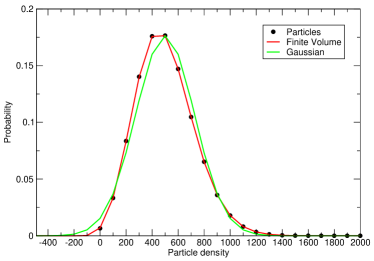
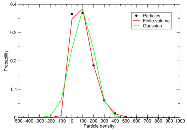
Figure 1: PDFs of particle, finite volume and Gaussian numerical methods at low number densities. Left is 5 particles per cells; right is 1 particle per cell

To quantify the differences in these distributions, we examine higher-order moments of the distribution. In Figure 2, we compute skewness and kurtosis of the equilibrium distributions for each method as a function of the number of particles per cell, again using a one dimensional problem with 100 zones. With 50 particles per zone, all of the methods predict a skewness close to zero and a kurtsosis of about three, corresponding to a Gaussian distribution. The Gaussian algorithm retains the Gaussian character (by construction) for all values of particles per cell. For the particle algorithm and the finite volume method, deviations from Gaussian begin to appear at 20 particles per cell and become significant at 10 particles per cell. The particle algorithm and the finite volume algorithm agree reasonably well at 10 particles per cell but begin to show discrepancies at 5 particles per cell that become more pronounced at 1 particle per cell.

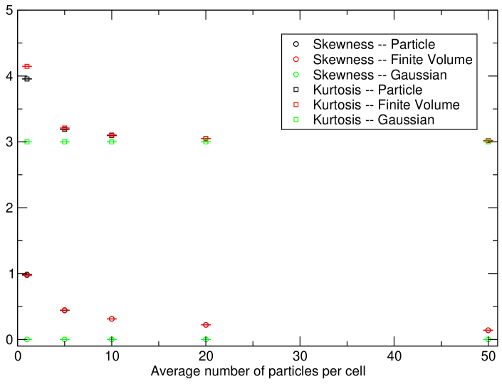
Figure 2: Skewness and kurtosis as a function of particles per cell

These higher-order statistics show that accuracy of finite volume SPDE description decreases as the number of particles per zone decreases. This allows us to establish a quantitative relationship between the number of particles per cell and breakdown in the accuracy of the finite volume discretization. The data in Figure 2 suggest that finite volume discretization begins to show significant errors with fewer than 5-10 particles per zone, suggesting 10 particles per zone is a reasonable value to use as a “refinement” criterion.

As an initial test of the hybrid, we consider a dynamic case in which particles are diffusing into an initially void region. We again consider a one-dimensional period case with 100 zones with $q=0$ for $0.25\leq x\leq 0.75$ and $q=2000$ elsewhere, corresponding to 20 particles per cell. For this test we fix the particle region to be one-cell wider in each direction than the region where there are initially no particles. In Figure 3 we present statistics for an ensemble of 20,000 simulations. The means and variances are in good agreement for all 4 methods. For the linearized Gaussian method, however, the skewness and kurtosis, which reflect a Gaussian distribution, are significantly different than the values for the particle algorithm, particularly in the low particle density region. The finite volume algorithm does somewhat better, however, the errors in the low particle density region are still significant. The hybrid algorithm captures the peaks in skewness and kurtosis at low particle densities, demonstrating that the hybrid algorithm can accurately model systems with regions of low particle density.

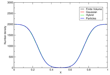
a) b)

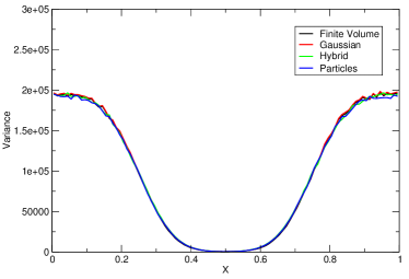
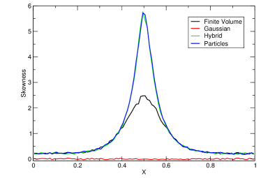
c) d)

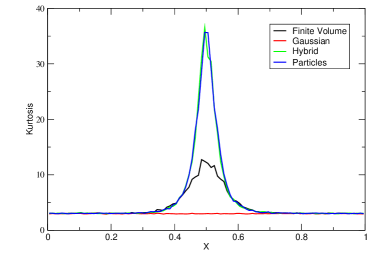
Figure 3: Ensemble average of dynamics of particles diffusing into a void region. (a) Mean, (b) Variance, (c) Skewness, and (d) Kurtosis

Next we consider examples in multiple dimension that demonstrate the dynamic adaptation of the methodology. The first example is a two-dimensional case with initial conditions given by an ellipsoidal region with 15 particles per cell surrounded by a larger elliptical region without any particles embedded in a background with 30 particles per cell, as illustrated in Figure 4. The simulation is performed on a $256\times 256$ grid. For the hybrid simulation we tag cells with fewer than 5 particles per cell to be in the particle region. We compare the hybrid using the finite volume discretization with the finite volume discretization in Figures 4 and 5. The inner ellipse is initially outside the particle region but as the system evolves the density decreases and the particle region expands to include the entire inner ellipse. At the outer edge of the larger ellipse, particles diffuse into the region and the particle region shrinks. Thus, this example shows regions entering and leaving the particle region. The hybrid algorithm and the finite volume algorithm produce similar large-scale features; however, the finite volume algorithm generates negative values (indicated by white dots in the figure) whereas the solution from the hybrid algorithm remains positive.

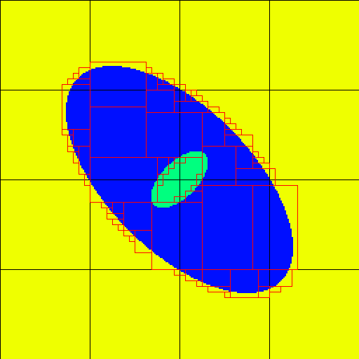
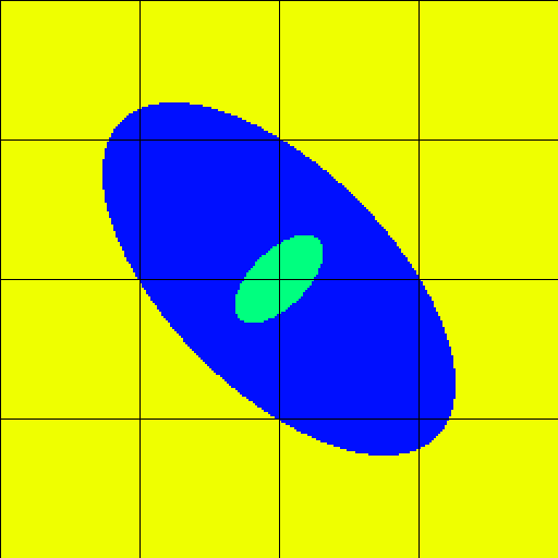
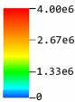
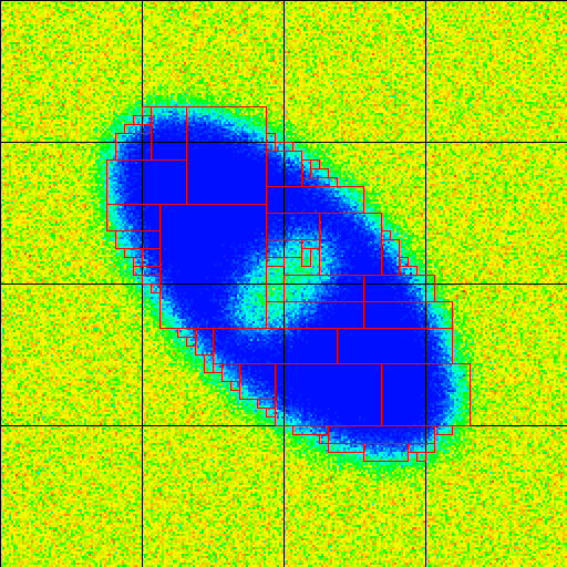
Figure 4: Time sequence comparing hybrid algorithm (left) with finite volume algorithm (right). The boxes outlined in red indicate the location of the particle region. White dots in finite volume algorithm indicate locations where the solution is negative. The hybrid solution remains positive. Times correspond to $t=0.$ and $t=0.00048$.

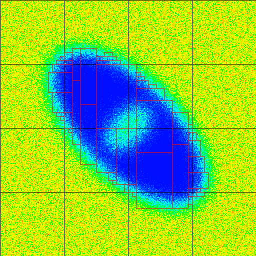
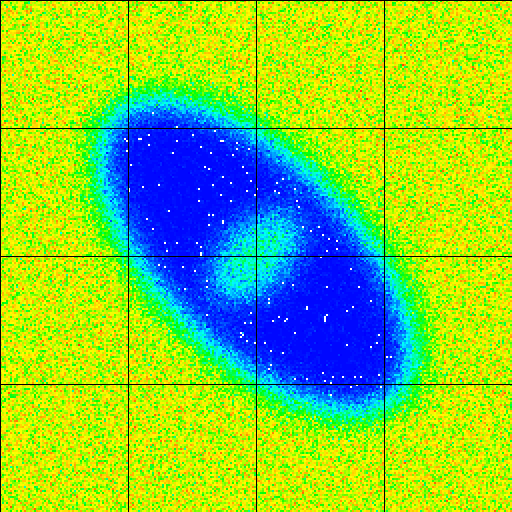
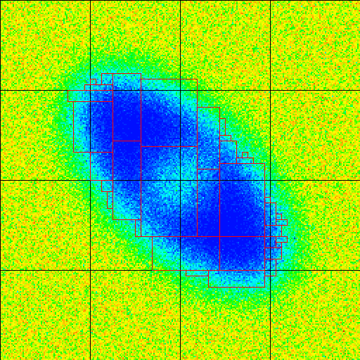
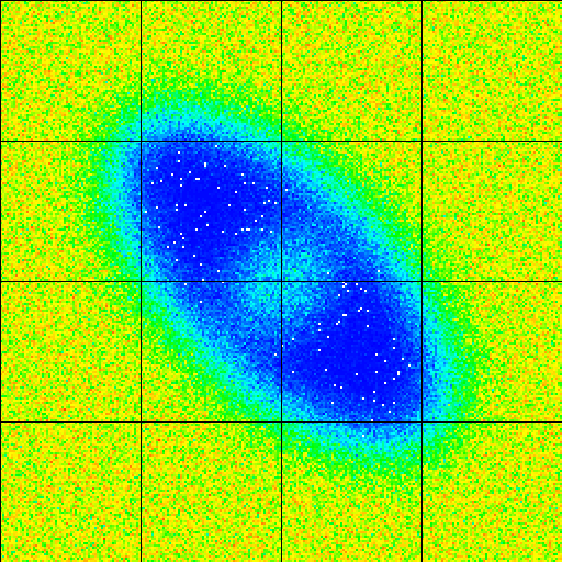
Figure 5: Continuation of time sequence comparing hybrid algorithm (left) with finite volume algorithm (right). The hybrid solution remains positive. Times correspond to $t=0.00096$ and $t=0.0024$.

The final example is a three-dimensional case with initial conditions given by a spherical region with 15 particles per cell surrounded by a larger spherical region without any particles embedded in a background with 30 particles per cell, as illustrated in Figure 6. The simulation is performed on a $128\times 128\times 128$ grid. As in the two dimensional case, we tag cells with fewer than 5 particles per cell to be in the particle region for the hybrid algorithm. Comparison of the hybrid with the finite volume discretization is presented in Figures 6 and 7. The inner sphere is initially outside the particle region. As the system evolves the density decreases and the particle region begins to expand. At $t=0.001$ only a small region of the inner sphere is still be modeled with the finite volume method. By $t=0.0015$ the particle region has grown to include the entire inner sphere. At the outer edge of the larger sphere, particles diffuse into the region and the particle region shrinks. The hybrid algorithm and the finite volume algorithm again produce similar large-scale features; however, the finite volume algorithm generates negative values (indicated by white dots in the figure) whereas the solution from the hybrid algorithm remains positive.

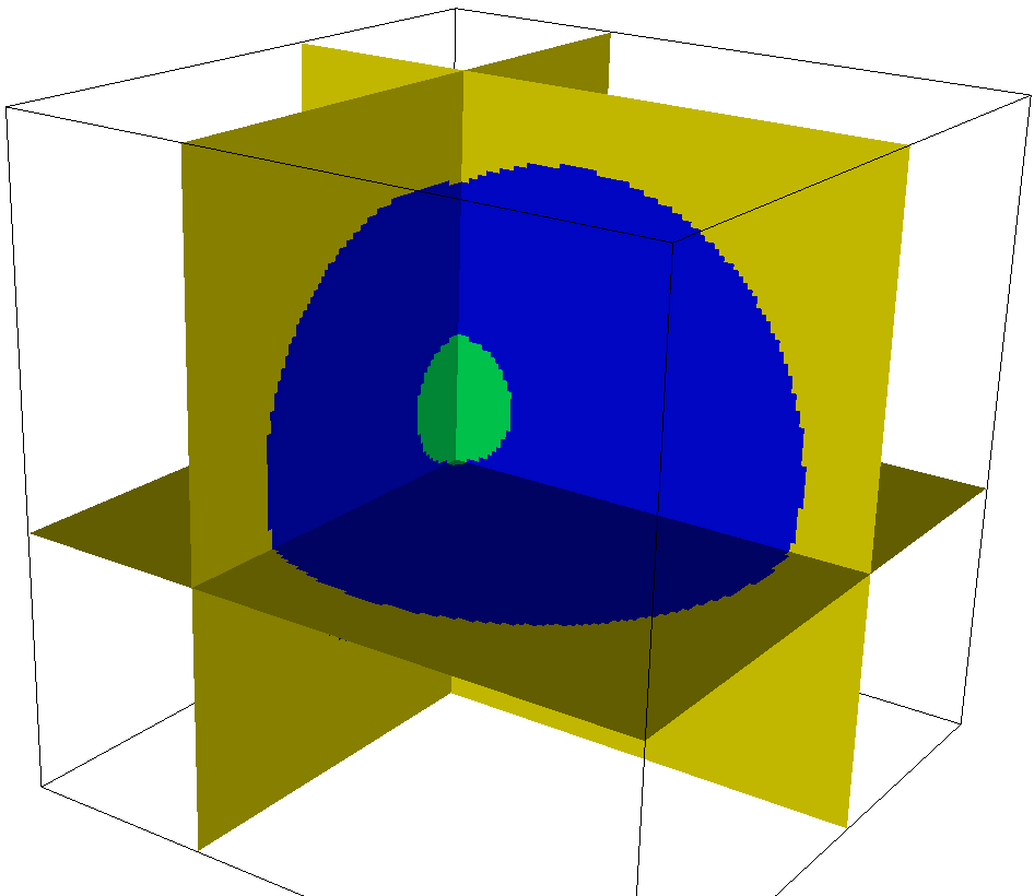
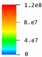
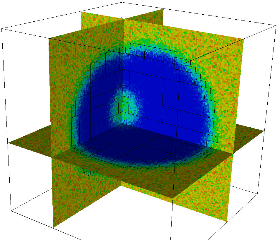
Figure 6: Time sequence comparing hybrid algorithm (left) with finite volume algorithm (right). The boxes outlined in black indicate the location of the particle region. White dots in finite volume algorithm indicate locations where the solution is negative. The hybrid solution remains positive. Times correspond to $t=0.$ and $t=0.001$.

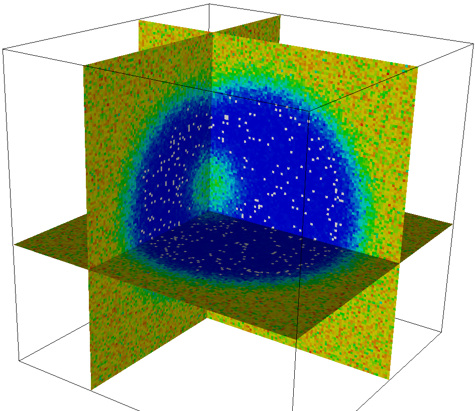
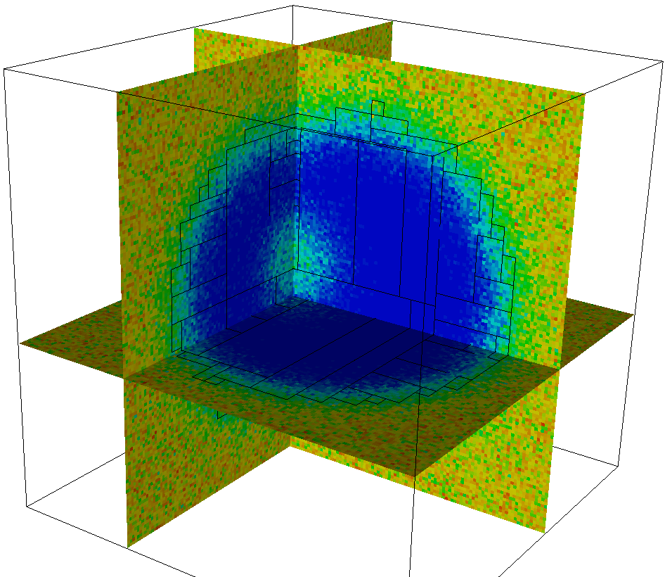
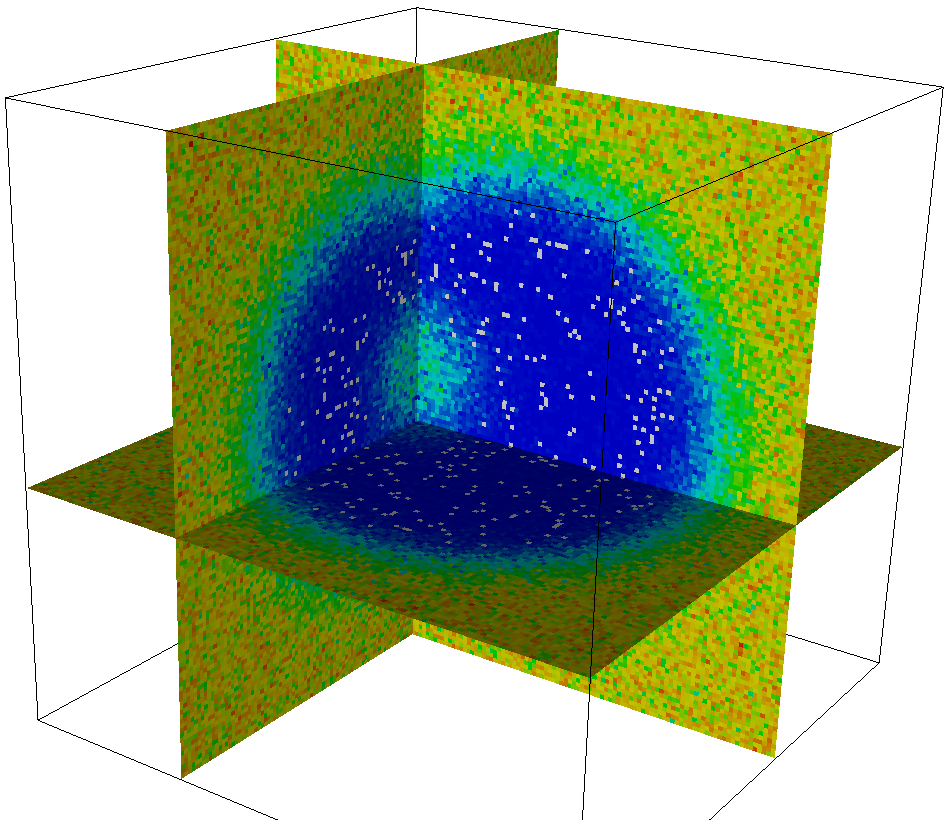
Figure 7: Continuation of time sequence comparing hybrid algorithm (left) with finite volume algorithm (right). The hybrid solution remains positive. Times correspond to $t=0.0015$, and $t=0.0025$.

5 Conclusions and further work

In this work we have presented a hybrid method for simulating the dynamics of non-interacting particles. This approach combines the simulation of the Dean-Kawasaki equation with truncated noise and particle dynamics in low-density regions. In particular, we developed the refinement criteria by comparing higher-order statistics. Compared to prior work on hybrid algorithms for particle systems, such as [1, 2], we focused specifically on regimes where particle density becomes low. In these regimes, our numerical experiments have shown that incorporating a particle description of the system is crucial for accurately preserving higher-order statistics and positivity of the solution. Additionally, we have extended the method to higher spatial dimensions with dynamic adaptation.

A next step is to consider higher-order time discretization methods, such as the Milstein scheme or the BDF2 method. Note that BDF2 is expected to provide higher accuracy for SPDEs with small noise, as discussed in [6]. Since the noise factor in Eq. (3) is $\frac{1}{\sqrt{N}}$, we expect to achieve higher-order accuracy when the number of particles is sufficiently large. It would be interesting to compare this threshold with the number of particles per cell required to ensure correct higher-order statistics and preserve the positivity of the solution.

We also aim to prove error bounds for the FVM applied to the modified equation from [12] and obtain a rate of convergence for the time discretization. Given that the modified equation has a well-behaved solution, we can directly analyze the error between the moments of the discretized and continuous solution, rather than using a weaker norm. Our goal is to compare how the choice of parameters determined by the discretization error aligns with the parameters chosen in [12] for the error between the modified and Dean-Kawasaki equations, as well as with the parameters obtained from simulations using the hybrid method. This type of analysis would allow us to link error estimates for the hybrid to the refinement criteria.

As observed in the simulations, it is not just the negativity of the solution that determines the choice of the particle description, but also the difference of the higher order statistics. An interesting question in this regard is how would the development of full discretization method of the SPDE that preserves the positivity of the solution influence the refinement criteria that we observed using standard FVM and Euler-Maruyama scheme.

The computational framework for hybrid algorithms developed here can be extended to a broader range of problems. As a first step in that direction, we plan to extend this hybrid method to interacting particle systems, incorporating an additional term $\nabla\cdot(\rho(\rho*\nabla U))$ in (3), where $U$ is the interaction potential. We will explore different interaction potentials, such as Coulomb or Leonard-Jones type, and study how these choices affect the refinement criterion.

Another promising application of the presented method is to study particles immersed within a surface, particularly for practical problems where geometry is crucial, as discussed in [22]. Our goal is to develop a hybrid method that incorporates the role of geometry by simulating the dynamics of Brownian particles on a surface, solving the corresponding stochastic equation on that surface, and synchronizing these processes while accounting for the geometric factors.

References

- [1] F. J. Alexander, A. L. Garcia, and D. M. Tartakovsky. Algorithm refinement for stochastic partial differential equations: I. linear diffusion. Journal of Computational Physics, 182(1):47–66, 2002.
- [2] F. J. Alexander, A. L. Garcia, and D. M. Tartakovsky. Algorithm refinement for stochastic partial differential equations. In AIP Conference Proceedings, volume 663, pages 915–922. American Institute of Physics, 2003.
- [3] A. J. Archer and M. Rauscher. Dynamical density functional theory for interacting Brownian particles: stochastic or deterministic? Journal of Physics A: Mathematical and General, 37(40):9325, 2004.
- [4] J. B. Bell, J. Foo, and A. L. Garcia. Algorithm refinement for the stochastic Burgers’ equation. Journal of Computational Physics, 223(1):451–468, 2007.
- [5] M. J. Berger and J. Rigoutsos. An algorithm for point clustering and grid generation. IEEE Transactions on Systems, Man, and Cybernetics, 21:1278–1286, 1991.
- [6] E. Buckwar and R. Winkler. Multistep methods for SDEs and their application to problems with small noise. SIAM journal on numerical analysis, 44(2):779–803, 2006.
- [7] F. Cornalba and J. Fischer. The Dean–Kawasaki equation and the structure of density fluctuations in systems of diffusing particles. Archive for Rational Mechanics and Analysis, 247(5):76, 2023.
- [8] F. Cornalba and T. Shardlow. The regularised inertial Dean–Kawasaki equation: discontinuous Galerkin approximation and modelling for low-density regime. ESAIM: Mathematical Modelling and Numerical Analysis, 57(5):3061–3090, 2023.
- [9] F. Cornalba, T. Shardlow, and J. Zimmer. Well-posedness for a regularised inertial Dean–Kawasaki model for slender particles in several space dimensions. Journal of Differential Equations, 284:253–283, 2021.
- [10] D. S. Dean. Langevin equation for the density of a system of interacting Langevin processes. Journal of Physics A: Mathematical and General, 29(24):L613–L617, Dec. 1996.
- [11] N. Dirr, B. Fehrman, and B. Gess. Conservative stochastic PDE and fluctuations of the symmetric simple exclusion process. arXiv preprint arXiv:2012.02126, 2020.
- [12] A. Djurdjevac, H. Kremp, and N. Perkowski. Weak error analysis for a nonlinear spde approximation of the Dean–Kawasaki equation. Stochastics and Partial Differential Equations: Analysis and Computations, pages 1–26, 2024.
- [13] N. Djurdjevac Conrad, J. Köppl, and A. Djurdjevac. Feedback loops in opinion dynamics of agent-based models with multiplicative noise. Entropy, 24(10):1352, 2022.
- [14] A. Donev, J. B. Bell, A. L. Garcia, and B. J. Alder. A hybrid particle-continuum method for hydrodynamics of complex fluids. Multiscale Modeling & Simulation, 8(3):871–911, 2010.
- [15] A. Donev, T. G. Fai, and E. Vanden-Eijnden. A reversible mesoscopic model of diffusion in liquids: from giant fluctuations to Fick’s law. Journal of Statistical Mechanics: Theory and Experiment, 2014(4):P04004, 2014.
- [16] A. Donev and E. Vanden-Eijnden. Dynamic density functional theory with hydrodynamic interactions and fluctuations. The Journal of chemical physics, 140(23), 2014.
- [17] A. L. Garcia, J. B. Bell, W. Y. Crutchfield, and B. J. Alder. Adaptive mesh and algorithm refinement using direct simulation Monte Carlo. Journal of computational Physics, 154(1):134–155, 1999.
- [18] L. Helfmann, N. Djurdjevac Conrad, A. Djurdjevac, S. Winkelmann, and C. Schütte. From interacting agents to density-based modeling with stochastic PDEs. Communications in Applied Mathematics and Computational Science, 16(1):1–32, 2021.
- [19] K. Kawasaki. Stochastic model of slow dynamics in supercooled liquids and dense colloidal suspensions. Physica A: Statistical Mechanics and its Applications, 208(1):35–64, 1994.
- [20] V. Konarovskyi, T. Lehmann, and M.-K. von Renesse. Dean-Kawasaki dynamics: ill-posedness vs. triviality. Electron. Commun. Probab., 24:1–9, 2019.
- [21] P. Martínez-Lera and M. De Corato. A finite element method for stochastic diffusion equations using fluctuating hydrodynamics. Journal of Computational Physics, 510:113098, 2024.
- [22] D. A. Rower, M. Padidar, and P. J. Atzberger. Surface fluctuating hydrodynamics methods for the drift-diffusion dynamics of particles and microstructures within curved fluid interfaces. Journal of Computational Physics, 455:110994, 2022.
- [23] N. Wehlitz, M. Sadeghi, A. Montefusco, C. Schütte, G. A. Pavliotis, and S. Winkelmann. Approximating particle-based clustering dynamics by stochastic PDEs. arXiv preprint arXiv:2407.18952, 2024.
- [24] W. Zhang, A. Myers, K. Gott, A. Almgren, and J. Bell. AMReX: Block-structured adaptive mesh refinement for multiphysics applications. The International Journal of High Performance Computing Applications, 35(6):508–526, 2021.