LLMs hallucinate graphs too:
a structural perspective

Abstract

It is known that LLMs do hallucinate, that is, they return incorrect information as facts. In this paper, we introduce the possibility to study these hallucinations under a structured form: graphs. Hallucinations in this context are incorrect outputs when prompted for well known graphs from the literature (e.g. Karate club, Les Misérables, graph atlas). These hallucinated graphs have the advantage of being much richer than the factual accuracy –or not– of a fact; this paper thus argues that such rich hallucinations can be used to characterize the outputs of LLMs. Our first contribution observes the diversity of topological hallucinations from major modern LLMs. Our second contribution is the proposal of a metric for the amplitude of such hallucinations: the Graph Atlas Distance, that is the average graph edit distance from several graphs in the graph atlas set. We compare this metric to the Hallucination Leaderboard, a hallucination rank that leverages $10,000$ times more prompts to obtain its ranking.

1 Introduction

Large Language Models (LLMs) recently attracted a lot of attention, thanks to sustained research efforts and a large spectrum of envisioned applications. This triggers a growing demand for tools to test and analyze these expensive to set up and complex objects. In particular, methods to efficiently identify, differentiate, watermark LLMs, and methods to compare their accuracy and notably the potential presence of hallucinations [15, 20, 19] are devised. The common denominator of these methods is the will to efficiently extract information from the LLM under scrutiny.

To achieve this information extraction, one can distinguish two broad categories of approaches: white box approaches that rely on exploiting a privileged access to the model internals (e.g. probits, activation patterns, source code, model hyperparameters and weights), and black box approaches that merely allow an auditor to interact with that model. White box approaches provide precise answers, but are not always available, for instance to an external auditor assessing a closed source LLM. In such cases, black box approaches are necessary, and constitute the focus of this paper.

To conduct a black box audit of a LLM, a common approach is to rely on multiple choice questions (MCQ) to test the accuracy of its answers. Using MCQ circumvents the difficulty and subjectivity of evaluating (potentially large numbers of) free text answers. To that end, several MCQ datasets are readily available, and cover a wide range of knowledge and reasoning domains. For instance, MedMCQA [17] contains 182k questions of 4 choices assessing the target model general medical knowledge. Using this dataset yields 2 bits of information about the target model per sent request. This might reveal inefficient if the auditor has to pay for each request or if the auditor has to limit the rate at which requests are sent.

In this paper, we explore a different approach using prompts willing to obtain graphs, rather than text. As graphs are structured, requesting graphs thus circumvents the problem of analyzing free form text answers. And most importantly, a single request to obtain a $n$ node graph from a LLM yields $O(n^{2})$ structured information bits from that model, enabling a much more efficient information extraction rate per request for the auditor. For instance, requesting the standard "Les Misérables" graph is much more efficient than issuing requests like "do Jean Valljean and Cosette both appear in a chapter?", for any two of the 77 characters of the book. Moreover, throughout the years, network science has produced a number of standard benchmark graphs already ingested by most LLMs, providing a readily available ground truth. This ingestion from LLMs comes from the fact that they are available as data online (e.g. in the SNAP [14] or KONECT [13] repositories among others), and as the process of training these LLMs is known to consume most of available data online [10].

While querying LLMs for graph structures is unexplored and might sound promising, it raises a number of questions we further investigate in the remainder of this paper. First, we detail the envisioned interaction framework in which the objective is to collect a graph as a LLM output. Once this basic interaction framework has been established, a first research question refers to the quality of the collected graphs. Namely, are output graphs accurate with regard to the original queried graph? And moreover, are some answers wrong and inaccurate, in other words do LLMs hallucinate graphs? Second, we showcase the potential of graph requests and their capacity to extract information regarding target LLMs in a request-efficient way. To that end, we compare our proposal (the Graph Atlas Distance) to the Hallucination Leaderboard [4].

2 The Topologies of LLM Graph Hallucinations

Our aim is to prompt LLMs with famous graphs for which the ground truth topology is known and available online (see e.g. on repositories such as SNAP [14] or KONECT [13]), and consequently most likely part of the training of these LLMs [10]. We chose three graphs in that regard, as ground truth: the Zachary’s karate club graph (coined KC hereafter) and Les Misérables (coined LM, see their composition e.g. in the NetworkX library [8]) and the 50th graph of the graph atlas [18].

Prompts to LLMs

Prompts to LLMs, in order to obtain a graph structure, are in the following form: Provide me the so called "X" graph as a python edge list; print it, with X being the graph of interest, for instance the "Zachary’s karate club", "Les Misérables" or Provide me with graph # from the Graph Atlas, as a python edge list; print it, with # the graph number in case of requests concerning the graph atlas. The request for Python structured responses is because of the NetworkX library [8] we use to instantiate and analyze these graphs.

Outputs by LLMs

Following such prompts, the returned payload is most often in the form of a list such as $(1,2),(1,3),\dots$ (see Section A for an example); that edge list is then parsed and built as a NetworkX graph (undirected ones in alignment with our ground truth graphs in this paper). As these ground truth graphs are also present in the NetworkX library, comparison is convenient. We note that incomplete outputs (i.e. incomplete responses leading to a partial edge list) are nevertheless examined. We report that a small fraction of queried LLMs refused return an edge list, as they claim not having access to the data for instance (as also noted by the Hallucination Leaderboard project [4]); some also prefer to provide Python code to print the queried graph using a library: these models are discarded from our study.

Prompted LLMs

The simplicity and low volume of necessary requests (prompts) enables a full online experience (as opposed to model downloading or API interfacing), using platforms that place LLMs in prompting access via a web browser. We leveraged the following platforms in this paper: Mistral [7], Vercel AI SDK [1], HuggingChat [5], ChatGPT [2], together.ai [9] and Google’s Gemini [3], with the default parameters the platforms set for their hosted models.

Comparing resulting graphs to the ground truth

In this paper we perform topological comparisons, with no consideration for the labels of nodes returned by the LLMs. These are varying significantly; in consequence a hard label matching would discard output graphs that are nevertheless topologically close. We leave a study on the labeling mismatch to future work.

2.1 Statistics on the Topology of Output Graphs by LLMs

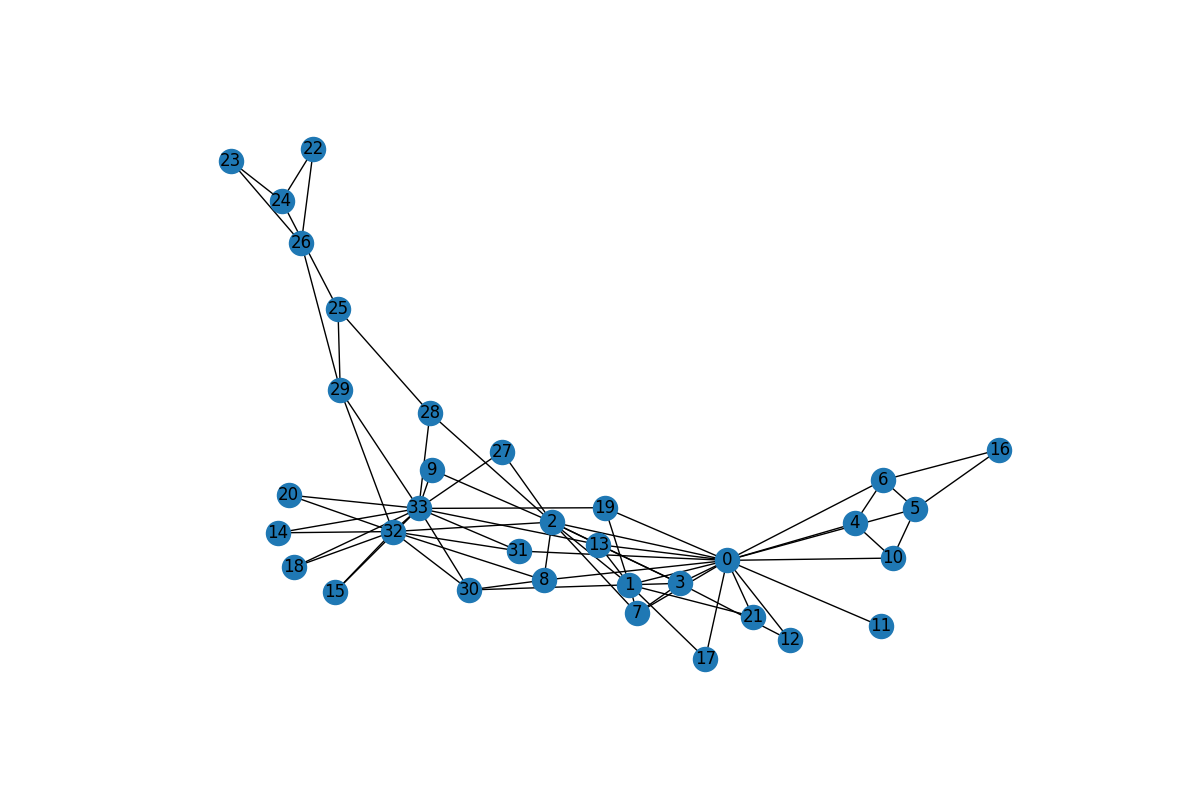
(a) Output graph

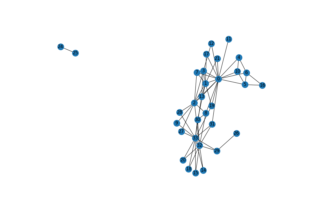
(b) Intersection

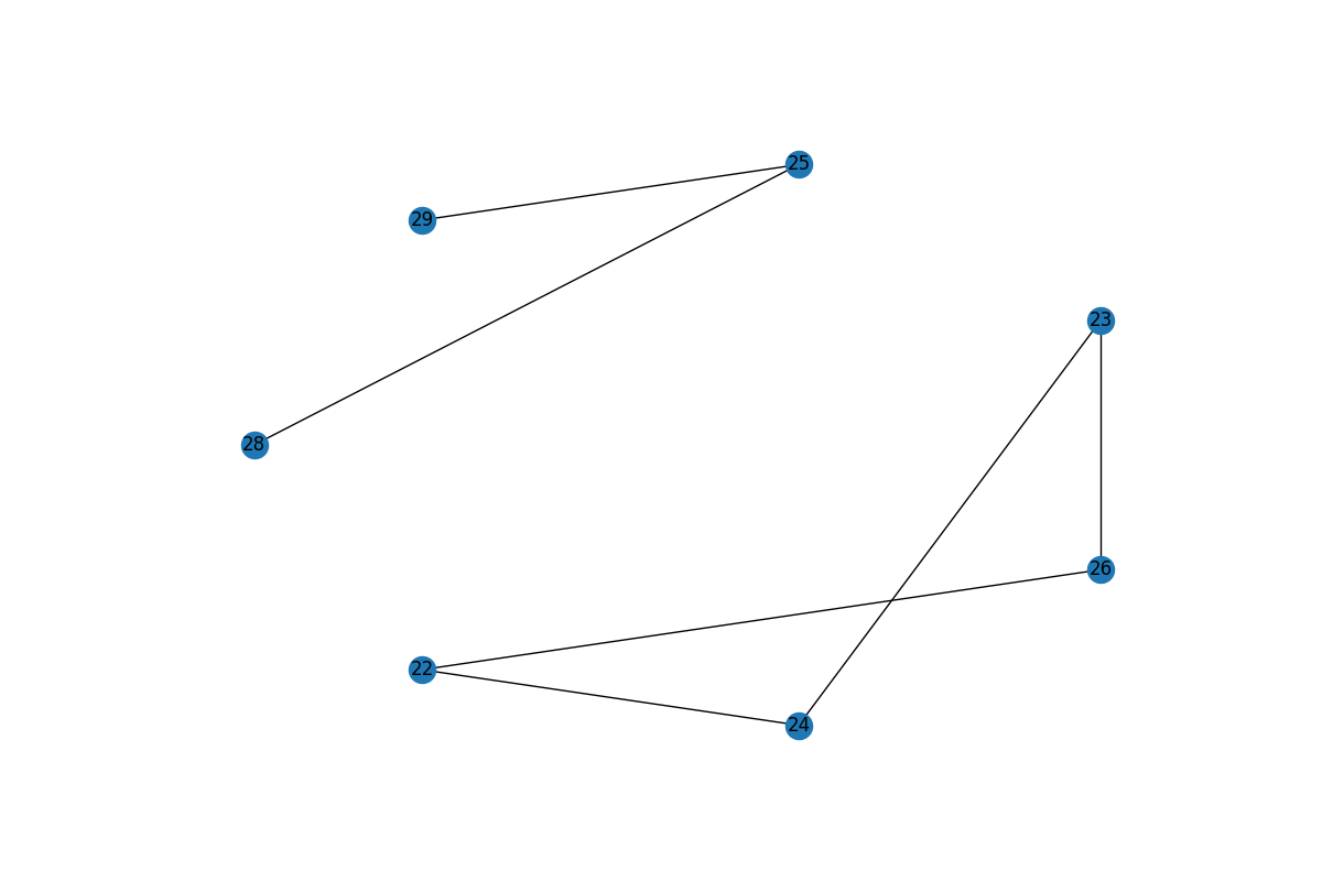
(c) Added edges

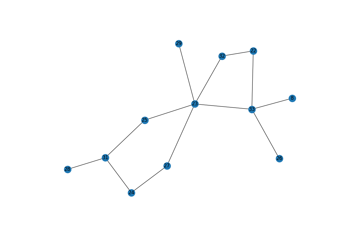
(d) Missing edges

Figure 1: Prompting gpt4o for the Zachary’s karate club graph: (a) answered output graph, (b) intersection of the output graph with the KC ground truth graph (a), (c) the edges added (hallucinated) w.r.t. to the KC graph, and (d) the edges missing w.r.t. the KC graph.

We report in detail the prompting of 21 LLMs against the Zachary’s karate club graph (KC); some statistics regarding Les Misérables and graph atlas 50 are deferred in Appendix B. As each prompt to a LLM results in a graph, one can directly perform topological comparison between the ground truth and a LLM output graph; such a comparison is represented in Figure 1: Figure 1a presents the raw output graph; Figure 1b presents the graph intersection of the KC graph with the output graph (from Figure 1a); Figure 1c presents the hallucinated edges (i.e. edges not present in KC but present in the output graph); finally Figure 1d presents the edges that are forgotten in the output graph as compared to KC, while prompting gpt4o. We note that the result provided by this LLM is relatively accurate in comparison to others, as we shall now see in Table 1.

LLM	|V|	|E|	density	assort.	modularity	dist. to KC deg. seq.
(reference: KC ground truth)	34	78	0.14	-0.48	0.31	0.0
dbrx-instruct	34	80	0.14	-0.47	0.15	2.0
gpt35	34	71	0.13	-0.41	0.36	3.74
gpt4o	34	71	0.13	-0.41	0.36	3.74
llama-3.1-70B-Instruct-Turbo	30	68	0.16	-0.29	0.4	8.6
gemini	16	21	0.17	-0.06	0.42	8.72
llama-3-8b-instruct	12	20	0.3	-0.0	0.29	10.0
llama-2-13b-chat-hf	6	8	0.53	-0.23	0.0	11.14
llama-3-sonar-small-32k-chat	13	31	0.4	-0.28	0.0	11.36
phi-3-mini-4k-instruct	9	15	0.42	-0.02	0.18	11.45
gemma-2-27b-it	8	13	0.46	-0.18	0.0	11.49
llama-2-70b-chat-hf	7	12	0.57	-0.14	0.0	11.79
llama-3.1-405B-Instruct-Turbo	23	57	0.23	-0.11	0.36	12.37
llama-3-sonar-large-32k-chat	14	38	0.42	0.05	0.0	13.42
llama-3-70B-Instruct-Turbo	22	77	0.33	0.07	0.28	14.14
llama-3-70B-Instruct-Lite	21	76	0.36	-0.0	0.0	14.73
llama-3-70b-instruct-groq	32	102	0.21	-0.13	0.43	15.36
snowflake-arctic-instruct	14	69	0.76	-0.28	0.0	16.0
c4ai-command-r-plus	28	139	0.37	-0.14	0.27	16.19
mistral-large	34	153	0.27	-0.12	0.4	18.49
qwen2-72B-Instruct	34	64	0.11	-0.97	0.0	22.18
llama-3.1-8B-Instruct-Turbo	39	77	0.1	-0.93	0.0	24.35

Table 1: The topological statistics of the output graphs returned by 21 LLMs when prompted for the Zachary’s karate club graph.

We denote the set $V$ of nodes and $E$ of edges in each examined graph. We name output graphs in relation with their LLM in the first column (in Table 1 the first row being the KC ground truth graph), and provide 6 relevant statistics for assessing their quality. From left to right, we list the number of nodes $|V|$ in the output graph, its number of edges $|E|$, its density, assortativity (tendency of nodes to attach to nodes with similar degrees), and modularity (that is computed w.r.t. the partition provided by a default label propagation on the output graph [8]). We argue modularity is an important indicator considering the frequent use of KC as a benchmark for community detection methods.

Finally we report in the last column the $l2$ distance between the degree distribution of the output graph and KC. Please note that except for rare unigraphic graphs, there exists multiple graphs having the same degree distribution, so this metric is not a correctness assessment per se. In other words, while strictly positive such distance implies a incorrect result, a distance of 0 does not imply a perfect (isomorphic to KC) result. The table is sorted using this last column.

Table 1 shows that no output graph is exactly correct: all LLMs do hallucinate. The closest one being by the dbrx-instruct model, with just two hallucinated (i.e. added) edges. ChatGPT models (3.5 and 4o) then follow and both return the same output graph. Many results are radically different from the correct one (hence deserving being coined hallucinations), with a surprisingly high heterogeneity among the answers (for instance, with $|E|$ ranging from 8 to 153).

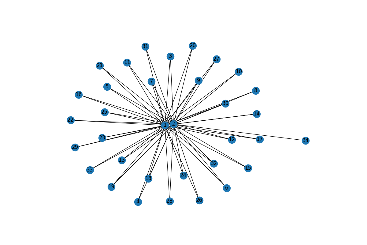
(a) qwen2-72B-instr.

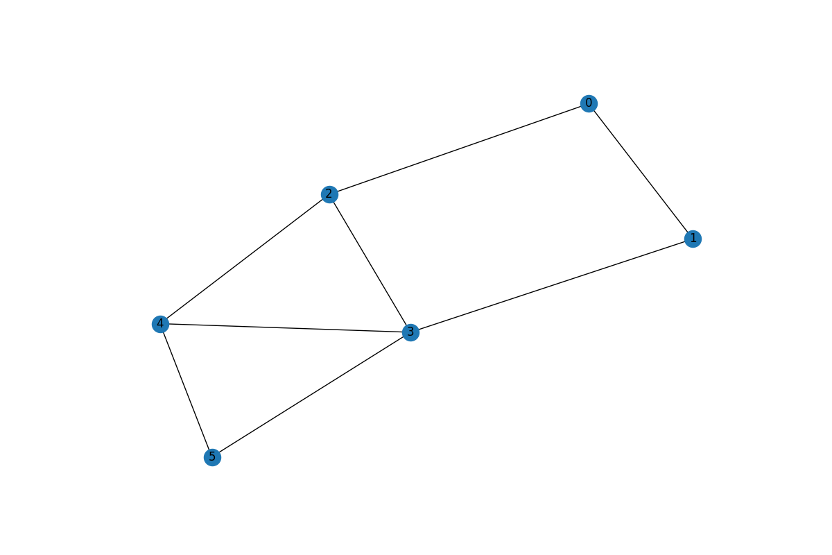
(b) llama-2-13b-chat-hf

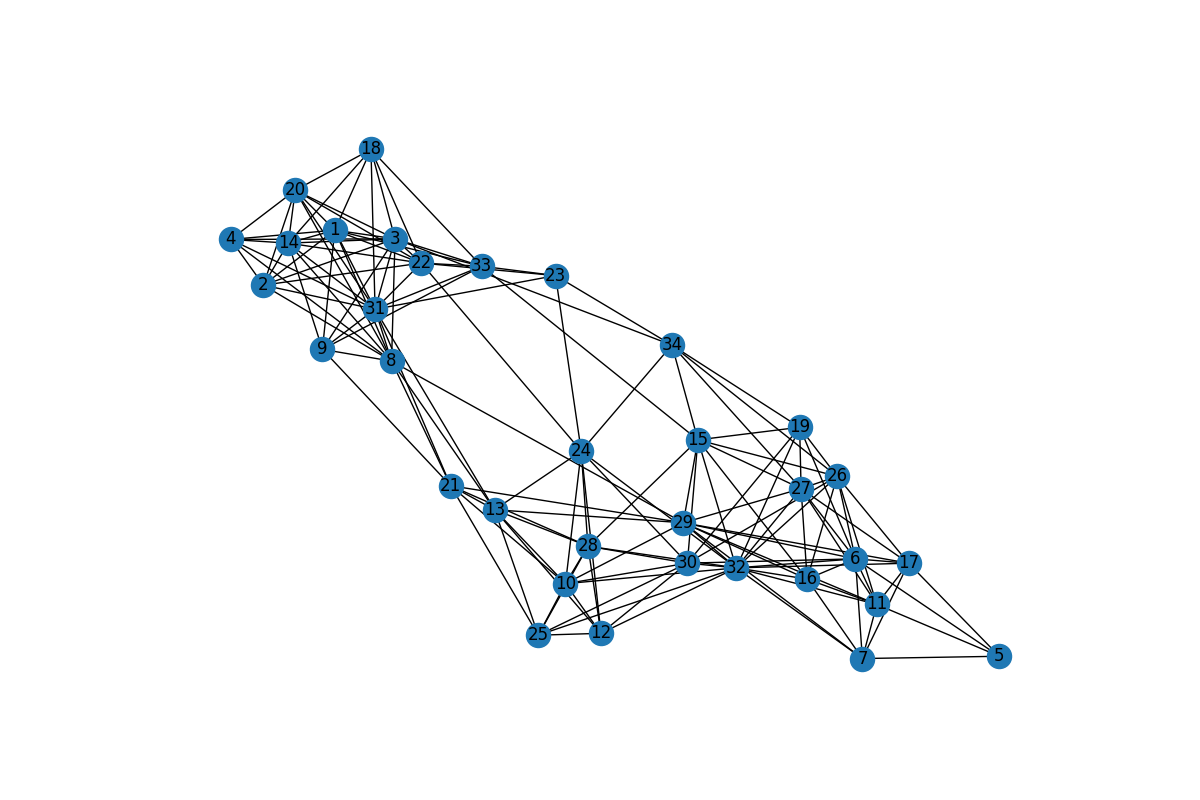
(c) mistral-large

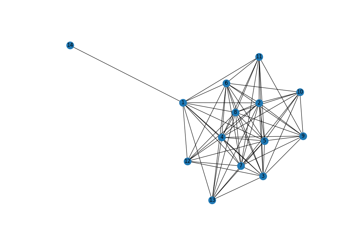
(d) snowflake-arctic-instr.

Figure 2: Example output graphs with salient particularities, when prompted for the Zachary’s karate club graph.

The bottom of the list is populated by output graphs that heavily differ from the ground truth, with i.e. the graph on Figure 2a that is a star with two central nodes (resulting in a low assortativity score). In this precise case, the number of nodes is correct, 34, and the number of edges close to correct, showing that model has probably learned these global features but not the topology. Figure 2b demonstrate the opposite case for llama-2-13b-chat-hf, where node and edge counts are very low (6 and 8 respectively). Another interesting case is mistral-large having the correct number of nodes while hallucinating nearly twice the number of edges (see Figure 2c), explaining its high distance to the degree sequence of KC, and its poor modularity in comparison. Finally, Figure 2d demonstrates for snowflake-arctic-instruct the output of a dense graph (except for a node, resulting in a high density).

On the model family side, we observe with llama variants that a higher amount of parameters does not imply more correctness: lama-3.1-405B-Instruct-Turbo is ranked in the middle in that regard. We also observe that for a model version (llama-3-70B), different variants (lite, turbo and groq) result in related ranks, yet with significantly different characteristic outputs.

2.2 Embedding LLMs Output Graph and the Ground Truth

We now rely on graph embeddings, for examining the relative proximity of LLM outputs. We employ the Karate Club library [6] for that purpose, with the NetLSD method [21] with default parameters, before we run a t-SNE appearing in Figure 3. (Les Misérables and graph atlas 50 are deferred in Appendix B.)

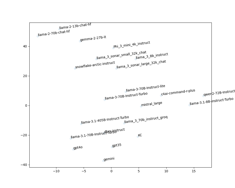
Figure 3: A t-SNE representation of the KC graph and of LLM outputs.

Despite the proximity of some related model architectures such as llama-2 or ChatGPT, a relatively smooth spread appear in this t-SNE, with clusters that mix graphs obtained by different vendors. Older versions of llama models (version 2) appear the less related to KC in this embedding.

3 A LLM Hallucination Rank Based on Output Graphs

Benchmarks for measuring hallucinations are constituted of tens of thousand of prompts [4, 17]. They hence require a privileged access to the model, compared to web browser based prompting access. We here propose to sequentially prompt a LLM for just a handful of graphs from the graph atlas, and to average errors made regarding this reference under a single value (using the average error of graph edit distances).

The graph atlas is composed by 1252 different graphs; in our experiment, we choose a resolution of $5$ graphs to be prompted, in particular the first $5$ connected graphs (namely graphs #3,#6,#7,#13 and #15). We then compute the exact edit distance of each of these ground truth graphs against their respective LLM output. We finally average these $5$ distances to obtain the final distance score for the queried LLM. We coin this distance the Graph Atlas Distance (GAD).

We note that across all tested LLMs and for all datasets, an isomorphism solely occurred for gpt4o on graph atlas #7 (a triangle graph) and #13 (a star composed of 4 nodes). Regarding the weight we give to operation in the graph edit distance, we do not account for labels, but consider node/edge insertion/deletion each costing 1.

We compare against the Hallucination Leaderboard [4], a GitHub page ranking LLMs based on the amplitude of their hallucinations, using a dataset of 50k prompts. The rank of the ten tested graphs in common with the Hallucination Leaderboard are presented in Table 4.

Rank	Graph Atlas Distance (GAD)	Hallucination Leaderboard$\star$
#1	gpt4o (2.2,2.16)	gpt4o
#2	llama-3.1-70B-Instruct (6.8,4.76)	snowflake-arctic-instruct
#3	llama-3-8b-chat-hf (8.0,2.34)	yi-1.5-34B-Chat
#4	llama-3.1-405B-Instruct-FP8 (8.2,2.16)	llama-3.1-405B-Instruct-FP8
#5	qwen2-72B-Instruct (8.4,2.3)	qwen2-72B-Inst
#6	yi-1.5-34B-Chat (9.4,2.19)	llama-3.1-70B-Instruct
#7	dbrx-instruct (10.0,5.78)	llama-3-8b-chat-hf
#8	llama-2-7b-chat-hf (17.2,7.52)	c4ai-command-r-plus
#9	snowflake-arctic-instruct (31.0,24.12)	dbrx-instruct
#10	c4ai-command-r-plus (38.0,41.74)	llama-2-7b-chat-hf

Figure 4: GAD (resolution: 5 graphs) vs a summarization of a benchmark based on prompts with binary answers [4]. In the GAD column, the first number is the average edit distance distance, the second is the standard deviation. ($\star$ rank in [4] as been adjusted to the LLMs available in our experiment)

We can observe an interesting correlation in these two rankings (with a spearman rank correlation of $0.3$, where $0$ is random). The first position is held by gpt4o. The first of the 4 llama models (llama-3.1-70B-Instruct) is down-ranked in GAD, yet the 3 others are in the correct order. The larger 405B parameters llama perform worse than smaller models; note that this inversion also appears in [4], where llama 3 beats llama 3.1 with the same amount of parameters (70B). qwen2-72B-Instruct ranks in the middle. c4ai-command-r-plus ranks at the bottom. snowflake-arctic-instruct is nevertheless strongly down-ranked with GAD, as compared to its second position in the Hallucination Leaderboard.

In the light of the only 5 graphs prompted to judge a LLM, and considering the 50k prompts in the Hallucination Leaderboard, we find this result to be encouraging for further study on the discriminative power of querying LLMs for structured data such as graphs.

4 Discussion

Reasoning, overfitting or hallucinating

So far, no LLM managed to consistently output the ground truth graphs. This might be considered as hallucinations, a sign that the LLMs handling of structures still needs to be improved. What is required from LLMs is yet not the overfitting and storage of input data, but rather to generalize from the provided examples. In this light, witnessing large blobs of (edgelist) text correctly returned by the LLM might be interpreted as an additional metric for overfitting.

Interestingly, the capacity to produce answers to a MCQ dataset like PiQa is interpreted as reasoning – rather than again overfitting –. In essence, reasoning could produce Les Misérables graph provided the original novel and the edge definition (chapter co-occurrence).

Gathering raw information, a meaningful abstraction ?

Our approach explores graph requests as a mean to obtain more information bits by prompt, compared to the standard MCQ approach naturally in which each request yields a number of bits capturing the number of possible answers to each question (typically 2 or 4 choices, hence 1 or 2 bits).

Implicitly, this approach hence compares interrogation patterns "bit to bit", regardless of the relevance of the collected bits. A natural limitation is to overlook the precise meaning of each bit. Concretely, for instance, one bit yielded by our approach captures whether the target LLM correctly predicted a (Jean Valjean, Cosette) relation in Les Misérables, whereas one bit yielded by MedMCQA benchmarks captures whether the target LLM correctly associates "A 40-year-old man has megaloblastic anemia and early signs of neurological abnormality" to a deficit in B12 Vitamin.

The difficulty with considering the semantics associated with each bit is that the notion of relevance is strongly application dependent. The relevance varies depending on the use case, be it for fingerprinting a target LLM or for evaluating its ability to provide truthful medical advice.

5 Related Work

Graphs are already used in various ways regarding the hallucination [15, 20, 19] issue, in order to assess properties or judge on the quality of outputs from LLMs.

Knowledge graphs are leveraged in a LLM-based hallucination evaluation framework [19], by prompting for text and checking the correctness of the output having a binary labeled dataset at hand. Knowledge graphs are constructed from unstructured textual data by identifying the set of entities within the text and the relationships between them, resulting in a structured representation.Work in [11] models social networks as graphs in order to simulate information spreading in order to track LLM hallucinations flowing within these networks. Nonkes et al. [16] create a graph structure that connects generations that lie closely in the embedding space of hallucinated and non-hallucinated LLM text generations. Graph Attention Networks then learn this structure and generalize it to unseen generations for categorization. Work in the complex networks community [12] is interested in extracting organizational networks (bipartite user-activity networks here) from raw text obtained from LLMs, in the context of standardized individual-level contributions across a large numbers of teams participating to a competition for instance.

To be best of our knowledge, our work is the first to propose a head-to-head comparison of a ground truth graph to a prompted output graph given by a LLM under scrutiny, allowing for new assessments.

6 Conclusion

This paper made the case for comparing ground truth graphs from the literature to the output of LLMs, prompted to output them. A first striking observation is that current LLMs are far from being a reliable source of edge lists (i.e. they do hallucinate graphs). Nevertheless, these glitches open solid comparison avenues, which we exploited to observe the significant differences of LLMs in their hallucination amplitude regarding standard graphs. Introducing relevant metrics, we have illustrated that a handful of prompts to a LLM can correlate with a method leveraging tens of thousands of queries for binary answers, in the capability to rank the less hallucinating LLMs. We believe that such a novel perspective leaves ways for future work to constitute robust and more efficient benchmarks for assessing the quality of LLMs.

Appendix A Example output from a LLM

We collected this example at the following url on the together.ai platform: https://api.together.xyz/playground/chat/meta-llama/Meta-Llama-3.1-405B-Instruct-Turbo, with the following prompt: Provide me the so called "Zachary’s karate club" graph as a python edge list; print it. Here is the full response from that model:

Zachary’s Karate Club is a well-known social network dataset that represents the friendships between 34 members of a karate club at a US university in the 1970s. The graph is often used as a benchmark for community detection algorithms.

Here is the graph represented as a Python edge list:

import networkx as nx

# Define the edge list
edges = [
    (1, 2), (1, 3), (2, 3), (1, 4), (2, 4), (3, 4), (1, 5), (2, 5), (1, 6), (3, 6),
    (1, 7), (5, 7), (6, 7), (1, 8), (2, 8), (3, 8), (1, 9), (3, 9), (3, 10), (3, 11),
    (1, 12), (1, 13), (4, 13), (3, 14), (3, 15), (6, 16), (6, 17), (7, 17), (6, 18),
    (1, 20), (2, 20), (1, 22), (2, 22), (24, 26), (25, 26), (3, 28), (3, 29), (3, 30),
    (24, 31), (27, 31), (2, 32), (24, 32), (2, 33), (4, 33), (24, 33), (25, 33),
    (26, 33), (27, 33), (28, 33), (29, 33), (30, 33), (31, 33), (32, 33)
]

# Create a graph from the edge list
G = nx.Graph(edges)

# Print the graph
print("Nodes:", G.nodes())
print("Edges:", G.edges())

import networkx as nx

# Define the edge list
edges = [
    (1, 2), (1, 3), (2, 3), (1, 4), (2, 4), (3, 4), (1, 5), (2, 5), (1, 6), (3, 6),
    (1, 7), (5, 7), (6, 7), (1, 8), (2, 8), (3, 8), (1, 9), (3, 9), (3, 10), (3, 11),
    (1, 12), (1, 13), (4, 13), (3, 14), (3, 15), (6, 16), (6, 17), (7, 17), (6, 18),
    (1, 20), (2, 20), (1, 22), (2, 22), (24, 26), (25, 26), (3, 28), (3, 29), (3, 30),
    (24, 31), (27, 31), (2, 32), (24, 32), (2, 33), (4, 33), (24, 33), (25, 33),
    (26, 33), (27, 33), (28, 33), (29, 33), (30, 33), (31, 33), (32, 33)
]

# Create a graph from the edge list
G = nx.Graph(edges)

# Print the graph
print("Nodes:", G.nodes())
print("Edges:", G.edges())

This code defines the edge list for Zachary’s Karate Club graph and creates a NetworkX graph object from it. The print statements display the nodes and edges of the graph.

Note that the node labels are integers from 1 to 34, and the edges represent friendships between the

Note that the response is cut as presented here (default output length on this platform is 512).

Appendix B Statistics and Embeddings for Les Misérables and Graph Atlas 50

LLM	|N|	|V|	density	assort.	modularity	dist. to LM deg. seq.
(reference: Les Misérables)	77	254	0.09	-0.17	0.46	0.0
gpt4o	66	180	0.08	-0.22	0.5	7.55
c4ai-command-r-plus	55	87	0.06	-0.57	0.11	17.49
llama-3.1-405B-Instruct-Turbo	26	38	0.12	-0.56	0.63	17.64
qwen2-72B-Instruct	25	33	0.11	-0.72	0.0	18.33
dbrx-instruct	9	11	0.31	0.16	0.29	22.76
gemini	14	15	0.16	-0.02	0.37	22.07
mistral-large	15	19	0.18	0.08	0.43	22.09
gemma-2-27b-it	14	25	0.27	-0.1	0.4	23.56
llama-3-70b-instruct-groq	24	47	0.17	0.11	0.59	23.35
phi-3-mini-4k-instruct	9	12	0.33	-0.21	0.21	23.07

Table 2: Statistics for graphs returned by 10 LLMs (Les Misérables).

LLM	|N|	|V|	density	assort.	modularity	dist. to ga50 deg. seq.
(reference: graph atlas 50)	5	8	0.8	-0.33	0.0	0.0
gemma-2-27b-it	5	7	0.7	-0.5	0.0	2.83
gpt4o	6	9	0.6	1.0	0.0	2.24
llama-3.1-405B-Instruct-Turbo	5	6	0.6	-0.29	0.0	2.0
c4ai-command-r-plus	5	10	1.0	1.0	0.0	5.66
llama-3-70b-instruct-groq	12	13	0.2	0.21	0.37	6.4
dbrx-instruct	10	45	1.0	1.0	0.0	10.82
qwen2-72B-Instruct	58	57	0.03	-0.26	0.65	37.22
mistral-large	100	375	0.08	-0.5	0.8	70.83

Table 3: Statistics for graphs returned by 8 LLMs (graph atlas #50).

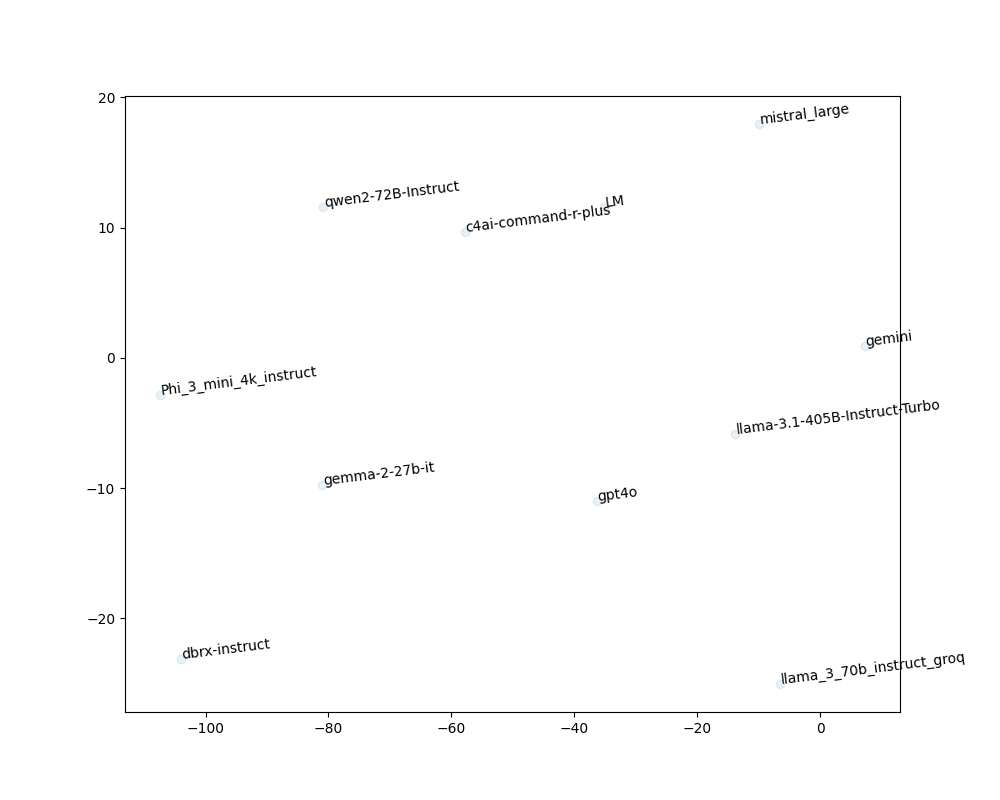
(a) Les Misérables graph

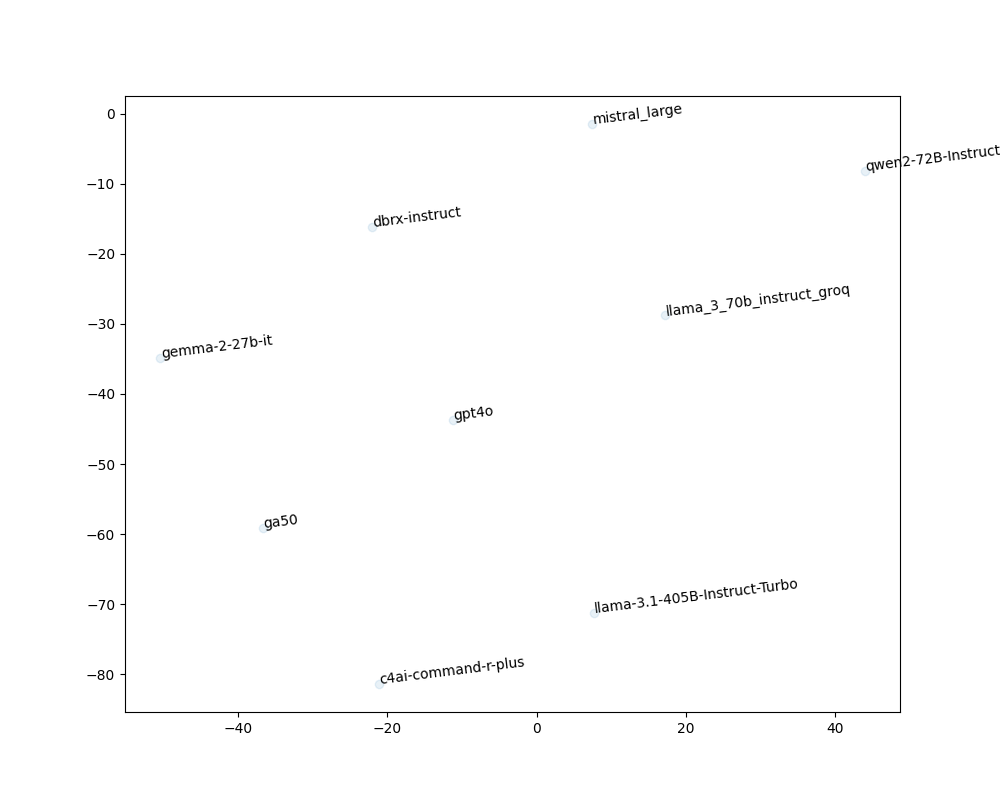
(b) Graph Atlas 50

Figure 5: t-SNE representation of graphs returned by the prompted LLMs.

Statistics related to Section 2 appear in Tables 2 and 3, as well as the embeddings for these 2 graphs in Figure 5.

Appendix C Spectral Distances from Ground Truth Graphs

Since the graph edit distance is intractable, even in practice from graphs with several tens of nodes, other related distances have been proposed, such as the spectral distance [22], defined as follows:

$$d(G,G^{\prime})=\sqrt{\Sigma_{i}(s_{i}-s^{\prime}_{i})^{2}},$$

with $s$ the set of eigenvalues $s=\{\lambda_{1},\lambda_{2},\dots,\lambda_{|V|}\}$, knowing that $\lambda_{1}\leq\lambda_{2}\leq\dots\leq\lambda_{|V|}$. As recommended in [22], if graphs are of different sizes, the missing eigenvalues of the smaller are zeros padded.

We report the spectral distances of LLMs to the KC graph in Table 4.

LLM	Spectral distance [22]
(reference: KC ground truth)	0
mistral-large	23.6
dbrx-instruct	27.34
gpt3.5	28.1
gpt4o	28.1
llama-3-70b-instruct-groq	32.64
qwen2-72B-Instruct	33.41
llama-3.1-70B-Instruct-Turbo	35.25
c4ai-command-r-plus	36.1
gemini	37.96
llama-3.1-405B-Instruct-Turbo	37.33
llama-3-70B-Instruct-Lite	37.63
llama-3-70B-Instruct-Turbo	37.81
llama-3-sonar-large-32k-chat	38.19
llama-3.1-8B-Instruct-Turbo	38.52
llama-3-sonar-small-32k-chat	38.6
llama-3-8b-instruct	38.61
phi-3-mini-4k-instruct	39.24
gemma-2-27b-it	39.32
llama-2-70b-chat-hf	39.54
llama-2-13b-chat-hf	39.6

Table 4: The spectral distance of the graphs returned by 21 LLMs when prompted for the Zachary’s Karate Club graph.

Note that as this distance is not the same as the distance between degree sequences from Table 1, we observe changes in the LLM ranking, such as with mistral-large leading Table 4. In this precise case, it appears that its high hallucination in the number of edges returned account less with this spectral metric.

References

- [1] The ai toolkit for typescript. https://sdk.vercel.ai. Accessed: 2024-08-20
- [2] Chatgpt. https://chatgpt.com. Accessed: 2024-08-20
- [3] Gemini. https://gemini.google.com. Accessed: 2024-08-20
- [4] Hallucination leaderboard. https://web.archive.org/web/20240820123721/https://github.com/vectara/hallucination-leaderboard. Accessed: 2024-08-20
- [5] Huggingchat. https://huggingface.co/chat/. Accessed: 2024-08-20
- [6] Karate club. https://github.com/benedekrozemberczki/karateclub. Accessed: 2024-08-20
- [7] Mistal ai. https://chat.mistral.ai. Accessed: 2024-08-20
- [8] Networkx, network analysis in python. https://networkx.org/. Accessed: 2024-08-20
- [9] together.ai. https://api.together.xyz/playground/chat. Accessed: 2024-08-20
- [10] Gao, L., Biderman, S., Black, S., Golding, L., Hoppe, T., Foster, C., Phang, J., He, H., Thite, A., Nabeshima, N., et al.: The pile: An 800gb dataset of diverse text for language modeling. arXiv preprint arXiv:2101.00027 (2020)
- [11] Hao, G., Wu, J., Pan, Q., Morello, R.: Quantifying the uncertainty of llm hallucination spreading in complex adaptive social networks. Scientific Reports 14(1), 16,375 (2024)
- [12] Jeyaram, R., Ward, R.N., Santolini, M.: Reconstructing networks from text using large language models (llms). In: The 12th International Conference on Complex Networks and their Applications (2023)
- [13] Kunegis, J.: Konect: the koblenz network collection. In: WWW (2013)
- [14] Leskovec, J., Krevl, A.: SNAP Datasets: Stanford large network dataset collection. http://snap.stanford.edu/data (2014)
- [15] Nadeau, D., Kroutikov, M., McNeil, K., Baribeau, S.: Benchmarking llama2, mistral, gemma and gpt for factuality, toxicity, bias and propensity for hallucinations (2024). URL https://arxiv.org/abs/2404.09785
- [16] Nonkes, N., Agaronian, S., Kanoulas, E., Petcu, R.: Leveraging graph structures to detect hallucinations in large language models. arXiv preprint arXiv:2407.04485 (2024)
- [17] Pal, A., Umapathi, L.K., Sankarasubbu, M.: Medmcqa: A large-scale multi-subject multi-choice dataset for medical domain question answering. In: Conference on health, inference, and learning, pp. 248–260. PMLR (2022)
- [18] Read, R.C., Wilson, R.J.: An atlas of graphs. Oxford University Press (1998)
- [19] Sansford, H., Richardson, N., Maretic, H.P., Saada, J.N.: Grapheval: A knowledge-graph based llm hallucination evaluation framework. arXiv preprint arXiv:2407.10793 (2024)
- [20] Tonmoy, S.M.T.I., Zaman, S.M.M., Jain, V., Rani, A., Rawte, V., Chadha, A., Das, A.: A comprehensive survey of hallucination mitigation techniques in large language models (2024). URL https://arxiv.org/abs/2401.01313
- [21] Tsitsulin, A., Mottin, D., Karras, P., Bronstein, A., Müller, E.: Netlsd: hearing the shape of a graph. In: Proceedings of the 24th ACM SIGKDD International Conference on Knowledge Discovery & Data Mining (2018)
- [22] Wilson, R.C., Zhu, P.: A study of graph spectra for comparing graphs and trees. Pattern Recognition 41(9), 2833–2841 (2008)