Prioritized Information Bottleneck Theoretic Framework with Distributed Online Learning for Edge Video Analytics
Abstract
Collaborative perception systems leverage multiple edge devices, such surveillance cameras or autonomous cars, to enhance sensing quality and eliminate blind spots. Despite their advantages, challenges such as limited channel capacity and data redundancy impede their effectiveness. To address these issues, we introduce the Prioritized Information Bottleneck (PIB) framework for edge video analytics. This framework prioritizes the shared data based on the signal-to-noise ratio (SNR) and camera coverage of the region of interest (RoI), reducing spatial-temporal data redundancy to transmit only essential information. This strategy avoids the need for video reconstruction at edge servers and maintains low latency. It leverages a deterministic information bottleneck method to extract compact, relevant features, balancing informativeness and communication costs. For high-dimensional data, we apply variational approximations for practical optimization. To reduce communication costs in fluctuating connections, we propose a gate mechanism based on distributed online learning (DOL) to filter out less informative messages and efficiently select edge servers. Moreover, we establish the asymptotic optimality of DOL by proving the sublinearity of their regrets. Compared to five coding methods for image and video compression, PIB improves mean object detection accuracy (MODA) while reducing 17.8% and reduces communication costs by 82.80% under poor channel conditions.
Index Terms:
Collaborative edge inference, information bottleneck, distributed online learning, variational approximations.I Introduction
I-A Background
Video analytics is rapidly transforming various sectors such as urban planning, retail analysis, and autonomous navigation by converting visual data streams into useful insights[2]. A large number of video cameras produce vast amounts of video data continuously and often require real-time video stream[3]. Numerous developing applications such as remote patient care[4], video games[5], and virtual and augmented reality depend on the efficient analysis of video data with minimal delay[6].
The increasing number of smart devices requires a computational paradigm shift towards edge computing. This approach involves processing· data closer to its source, resulting in several benefits compared to traditional cloud-based paradigms, particularly reduced latency and bandwidth costs. Even a delay as short as second can lead to disastrous consequences. For example, interactive applications such as online gaming and video conferencing require latencies below 100 ms to ensure real-time feedback and seamless user experience[7]. Similarly, VR/AR applications demand extremely low latencies, often less than 20 ms, to prevent motion sickness and maintain a high-quality immersive experience[8]. Utilizing remote cloud services for data processing can result in significant latency increases, often exceeding 100 ms[9]. Moreover, the importance of privacy, particularly in regions with strict data protection laws such as the General Data Protection Regulation (GDPR), makes edge computing even more attractive[10]. According to the Ponemon Institute, 60% of companies express apprehension toward cloud security and decide to manage their own data onsites in order to mitigate potential risks[11].
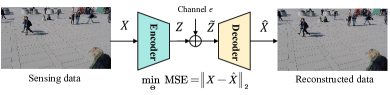
However, the integration of edge devices into video analytics also brings in many significant challenges[12]. The computational demands of deep neural network (DNN) models, such as GoogLeNet[13], which requires about 1.5 billion operations per image classification, place a substantial burden on the limited processing capacities of edge devices[14]. Additionally, the outputs from high-resolution cameras increase the communication load. For example, a 4K video stream requires up to 18 Gbps of bandwidth to transmit raw video data, potentially overwhelming wireless networks[15]. Therefore, we need to explore efficient video coding for compressing streamed videos. As shown in Fig. 1(a), the traditional compression is to reconstruct streaming frame through efficient entropy coding and motion prediction. However, there are still extensive less informative data being processed, wasting communication bandwidth. For instance, if the tasks involve human recognition or positioning, the reconstructed background of each frame might not be useful for the application.
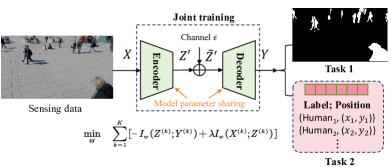
As shown in Fig. 1(b), the information bottleneck (IB) framework is a feasible choice for task-oriented video compression, enabling a trade-off between communication cost and prediction accuracy for specific tasks. However, the current communication strategies for integrating edge devices into video analytics are not effective enough. One major issue is how to handle the computational complexity and transmission of redundant data generated from the overlapping fields of view (FOVs) from multiple cameras[16]. In scenarios with dense camera deployments, up to 60% of data can be redundant due to overlapping FOVs, which unnecessarily overburdens the network[17]. In addition, these strategies often lack adaptability in transmitting tailored data features based on Region of Interest (RoI) and signal-to-noise ratio (SNR), resulting in poor video fusion or alignment. These limitations can negatively impact collaborative perception, even making it less effective than single-camera setups[18].
In this paper, we aim to refine multi-camera video analytics by developing a strategy to prioritize wireless video transmissions. Our proposed Prioritized Information Bottleneck (PIB) strategy attempts to effectively leverage SNR and RoI to selectively transmit data features, significantly reducing computational load and data transmissions. Our method can decrease data transmissions by up to 82.80%, while simultaneously enhancing the mean object detection accuracy (MODA) compared to current state-of-the-art techniques. This approach not only compresses data but also intelligently selects data for processing to ensure only relevant information is transmitted, thus mitigating noise-induced inaccuracies in collaborative sensing scenarios. This innovation sets a new benchmark for efficient and accurate video analytics at the edge.
I-B State-of-the-Art
This subsection reviews advancements in edge video analytics, with an emphasis on the designs on communication-computing latency reduction. We explore the information bottleneck method to enhance task-oriented performance by minimizing data redundancy. Additionally, we investigate online learning for dynamic ROI management and perceptual quality.
I-B1 Edge Video Analytics
Live video analytics is crucial in various domains such as autonomous driving[18, 19, 20, 21, 22, 23], mixed reality[24, 25], 3D point cloud analytics[26], and traffic control[27]. These applications, including object recognition[28], are typically equipped with sophisticated machine learning models like Convolutional Neural Networks (CNNs)and Graph Neural Networks (GNNs)[29, 30]. However, offloading these applications to central clouds can result in unpredictable transmission delays in wide area networks, particularly when streaming high-quality videos[31]. Therefore, researchers utilize edge computing to serve as a promising alternative to reduce service latency and energy consumption. Li et al. propose a novel approach called ESMO to optimize frame scheduling and model caching for edge video analytics[32]. Khani et al. introduce RECL, a new framework for video analytics that integrates model reuse and online retraining to quickly adapt expert models to specific video scenes, optimizing resource allocation and achieving substantial performance gains over prior methods[33]. Wang et al. design an MEC-enabled multi-device video analytics system using a Markov decision process to address real-time ground truth absence and content-varying degradation-accuracy issues that significantly enhances the accuracy-latency tradeoff through adaptive information gathering and efficient bandwidth allocation. However, few works consider how to strike a dynamic balance between channel resources and inference performance in a multi-camera sensing system.
In typical edge video analytics scenarios, the lack of infrastructure and limited bandwidth makes real-time object detection challenging, especially for the multi-view camera sensing for wild animals or criminals in remote areas[34]. To achieve real-time object sensing, it is crucial to reduce redundant information and the bandwidth resource demand. Semantic communication can address this challenge by transmitting only the essential semantic information, thereby compressing data streams and reducing transmission overhead. Zhang et al. propose a comprehensive framework to highlight the importance of semantic communication in optimizing information transmission[35]. Shao et al. introduce a new conceptualization of semantic communication that characterizes it within joint source-channel coding theory, aiming to minimize the semantic distortion-cost region[36]. Xie et al. explore a deep learning-based semantic communication system with memory, showing how dynamic transmission techniques can enhance transmission reliability and efficiency by masking unessential elements[37]. Zhou et al. design and implement a deep learning-based image processing pipeline on the ESP32-CAM, proposing a DRL-based approach for efficient camera configuration adaptation in multi-camera systems[38]. Existing research primarily focuses on rate-distortion (R-D) optimization, adapting the bitstream rate based on channel state information (CSI) to reconstruct raw videos[39]. However, these methods rarely consider the performance of specific downstream tasks, such as mean object detection accuracy (MODA), as a system evaluation metric. Consequently, the transmitted information often contains redundant data.
To address this issue, researchers incorporate the information bottleneck (IB) framework to optimize edge video analytics by focusing on task-specific performance, thereby reducing redundancy[40]. The IB framework helps the cause in selectively transmitting only the most relevant features needed for specific tasks, enhancing efficiency. Pensia et al. propose a novel feature extraction strategy in supervised learning that enhances classifier robustness to small input perturbations by incorporating a Fisher information penalty into the information bottleneck framework[41]. Wang et al. present a deep multi-view subspace clustering framework to extend the information bottleneck principle to a self-supervised setting, leading to superior performance in multi-view subspace clustering on real-world datasets[42]. IB tradeoff is well-suited for bandwidth-limited edge inference and is a key design principle in our study for efficient communication. Wang et al. introduce the Informative Multi-Agent Communication (IMAC) method, which uses the information bottleneck principle to develop efficient communication protocols and scheduling for multi-agent reinforcement learning under limited bandwidth[43]. Shao et al. propose a task-oriented communication scheme for multi-device cooperative edge inference, optimizing local feature extraction and distributed feature encoding to minimize data redundancy and focus on task-relevant information, leveraging the information bottleneck principle and extending it to a distributed deterministic information bottleneck framework. However, these existing studies often neglect the need to prioritize different data from multiple cameras for various downstream tasks, such as considering ROIs. Moreover, most existing studies overlook the correlation between multiple cameras in multi-view scenarios. Shao et al. extract compact task-oriented representations based on the IB principle, but they overlook the fact that different tasks require varying levels of priority[12]. By leveraging these correlations and levels of priority, it is possible to further reduce data rates by minimizing duplicate information across different camera feeds and enhance inference performance at the same time.
I-B2 Learning-Based Transmission Scheduling
Online learning in multi-agent deep reinforcement learning (MADRL) enhances multi-camera sensing under dynamic channels and overlapped ROIs. Effective transmission scheduling determines when and which agents communicate through binary vectors indicating allowed communications at specific time steps, forming a communication graph. Central transmission scheduling schemes use a globally shared policy to control communication. Kim et al. propose SchedNet, which uses a global scheduler to limit broadcasting agents and reduce communication overhead[44]. Du et al. introduce FlowComm, forming a directed graph for communication[45]. Liu et al. develop GA-Comm, using a two-stage attention network (G2ANet) to manage agent interactions[46]. Niu et al. present MAGIC, a framework using a directed communication graph for enhanced coordination[47]. In distributed transmission scheduling schemes, each agent individually determines whether to communicate, forming a graph structure. Liu et al. propose a framework for multi-agent collaborative perception, addressing communication group construction and decision-making for efficient bandwidth use, significantly reducing communication while maintaining performance[48]. Deep learning optimizes these systems by refining communication actions and schedules, transmitting only relevant information, and minimizing redundancy. However, existing multi-camera cooperative sensing algorithms do not effectively address the transmission scheduling problem, particularly under dynamic wireless channels and overlapped ROIs.
I-C Our Contributions
Edge computing plays a crucial role in collaborative perception systems, improving tracking precision and minimizing blind spots through multi-view sensing. However, challenges such as limited channel capacity and data redundancy impede their effectiveness. To address these issues, we propose the Prioritized Information Bottleneck (PIB) framework for edge video analytics. Compared with the conference version[1], this paper improves the MODA by up to 17.88% and reduces the communication cost by 23.94%. Our contributions are summarized as follows:
-
•
We propose the PIB framework that prioritizes the share data based on the signal-to-noise ratio (SNR) and camera coverage of the region of interest (RoI), reducing redundancy both spatially and temporally. This approach avoids the need for video reconstruction at edge servers and maintains low latency.
-
•
Our framework leverages a deterministic information bottleneck method to extract compact, relevant features, balancing informativeness and communication costs. For high-dimensional data, we apply variational approximations for practical optimization.
-
•
To reduce communication costs in fluctuating links, we introduce a gate mechanism based on distributed online learning (DOL) to filter out unprofitable messages and efficiently select edge servers. We establish the asymptotic optimality of DOL by showing the sublinearity of their regrets.
-
•
Our extensive experimental evaluations demonstrate that PIB significantly enhances mean object detection accuracy (MODA) and reduces communication costs. Compared to TOCOM-TEM, JPEG, H.264, H.265, and AV1, PIB improves MODA by 17.8% while reducing communication costs by 82.80% under poor channel conditions. Additionally, our method can reduce the standard deviation of streaming packet sizes by up to 9.43%, while simultaneously maintaining higher MODA, ensuring better transmission robustness under poor channel conditions.
The remainder of this paper is organized as follows: Sec. II introduces the system model. Sec. III covers the problem formulation, including prioritized information bottleneck analysis and the CMAB problem. Sec. IV describes the methodology, focusing on the derivation of the IB problem’s upper bound, loss function design, and the distributed gate mechanism. Sec. V evaluates the performance of the PIB framework through simulations that forecast pedestrian occupancy in urban settings, considering communication bottlenecks, camera delays, and edge server connectivity.
II System Model
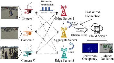
As illustrated in Fig. 2, our system comprises a set of edge cameras, denoted as , and a set of edge servers, denoted as . Each camera has a specific Field of View (FoV), , covering a subset of the total monitored area. In a high-density pedestrian environment, our goal is to facilitate collaborative perception for pedestrian occupancy prediction, under the constraints of limited channel capacity due to poor channel conditions. Moreover, the aggregate server is the central fusion edge server selected to minimize overall system delay. Other edge servers relay their data to this server for inference.
II-A Communication Model
We use Frequency Division Multiple Access (FDMA) to manage communication among cameras, defining the capacity for each camera and edge server combination using the SNR-based Shannon capacity:
| (1) |
where is the bandwidth allocated to the link between camera and edge server , and is the signal-to-noise ratio of this link. The transmission delay is given by:
| (2) |
where is the data packet size. Each camera decides whether to transmit data directly to its aggregate server or via a relay edge server based on channel quality: 1) If the channel quality is good, the camera transmits directly to the aggregate server . The total delay is , where is the inference delay at the aggregate server. 2) If the channel quality is poor, the camera first transmits to a relay edge server , which then forwards the data to the aggregate server. The total delay in this case is , where is the relay delay. By dynamically choosing between relay and direct transmission, the system adapts to varying channel conditions, ensuring minimal delays and efficient use of network resources.
II-B Priority Weight Formulation
Dynamic priority weighting is essential for optimizing network resource allocation, as various data sources require different levels of attention. Inspired by our previous work[18], we employ a dual-layer Multilayer Perceptron (MLP)111The MLP is trained in a supervised learning manner, where the input features are the normalized delay and the normalized number of perceived moving objects . The target output is the optimal priority weight . The loss function used for training is designed to minimize the discrepancy between the computed weights and the target weights , as described in Sec. IV-D. to compute priority weights based on normalized delay and the number of perceived objects ():
| (3) |
where denotes the computed priority score for camera , and represents the trainable parameters of MLP. The architecture of this MLP, featuring two layers, allows it to effectively model the interactions between delay and the number of perceived moving objects. Specifically, and , where represents the number of moving objects perceived by camera , while and denote the upper and lower bounds of the number of moving objects that any edge camera should perceive, respectively.
To transform the raw priority scores into a usable format within the system, we apply a softmax function, which normalizes these scores into a set of weights summed to one:
| (4) |
where signifies the priority weight for camera . This method ensures that cameras which are more critical, either due to high coverage or due to lower delays, are given priority, thereby enhancing the decision-making capabilities and responsiveness of the edge analytics system.
III Problem Formulation
In this section, we establish the theoretical foundation for our PIB framework. We begin by detailing the IB analysis to determine the optimal balance between data compression and relevant information retention. Following this, we formulate the combinatorial multi-armed band (CMAB) problem to model the decision-making process of cameras in a distributed environment.
III-A Prioritized Information Bottleneck Analysis
In the context of information theory, the IB method seeks an optimal trade-off between the compression of an input variable and the preservation of relevant information about an output variable [49]. Throughout this paper, upper-case letters (e.g., , , and ) represent random variables, while lower-case letters (e.g., , , and ) denote their realizations. We formalize the input data from camera as , and the target prediction as , corresponding to the population in the dataset . The goal is to encode into a meaningful and concise representation , which aligns with the hidden representation that captures task-relevant features of multi-view content for prediction tasks. The classical IB problem can be formulated as a constrained optimization task:
| (5) | ||||
| s.t. |
where denotes the mutual information between two random variables and . represents the set of all learnable parameters in the PIB framework, including and the variational approximation in the following section. The mutual information is essentially a measure of the amount of information obtained about one random variable through the other random variable. is the maximum permissible mutual information that can contain about . The objective is to ensure that captures the most relevant information about for predicting while remaining as concise as possible. By introducing a Lagrange multiplier222All Lagrange multipliers are the same, and we only use trainable weight parameters to dynamically balance between accuracy and communication bottleneck. , the problem is equivalently expressed as:
| (6) |
where represents the IB functional, balancing the compression of against the necessity of accurately predicting . Next, we extend the IB framework to a multi-camera setting by introducing priority weights to the mutual information terms, adapting the optimization problem as follows:
| (7) |
where the weighted mutual information terms are defined as follows:
| (8) |
where the non-negative value represents the maximum allowable weight for . The first term with linear weights is the weighted mutual information between the compressed representation from camera and the target . This term can also be used to capture the semantic compression in raw data. The linear weighting with ensures the influence of each camera is proportional to its priority weight. Higher values increase the weight given to in the objective function, emphasizing cameras that provide high-quality data for accurate target prediction.
The second term with negative exponential weights denotes the mutual information between the original data and its compressed form , scaled by a negative exponential function of . This ensures an exponential decay in the influence of as increases. Cameras with lower priority weights (lower ) undergo more aggressive data compression (as is greater for smaller values), optimizing bandwidth and storage usage without significantly affecting overall performance. In this paper, we use this type of weighting for the proof of concept study and will investigate more general weighting in the future.
III-B Combinatorial Multiarmed Bandit (CMAB) Problem
In dynamic environments with varying channel states and regions of interest (ROIs), ensuring high inference accuracy is challenging. The system must adaptively determine whether each camera should transmit its features and decide which edge server to use for transmission. Moreover, due to the edge server’s limited bandwidth and computing capacity, each camera must decide if it should transmit directly to an edge server or use another edge server as a relay node before data fusion at the final edge server.
Accordingly, the problem can be formulated as a combinatorial multi-armed bandit (CMAB) problem. Each camera’s connection establishment and edge server’s connection establishment are base arms, and the collective actions of all agents constitute a super arm. Let represent the action taken by camera at time , where denotes the connection between the -th camera and the -th edge server, and denotes the connection between the -th edge server and the -th edge server for data fusion. The super arm is a subset of arms selected for the decision to transmit (the -th edge server) and data fusion (the -th edge server)333We omit “” for simplicity in the definition of connection establishment.. Dynamic channel state and ROI impact inference accuracy. This metric can be defined using the change in Multiple Object Detection Accuracy (MODA). MODA is calculated as , where denotes the number of correctly detected objects, means the number of missed detections, and is the number of false detections. Specifically, the gain in MODA from adding the -th camera’s feature to the ego camera’s444The ego edge camera is the reference camera selected for data fusion. It typically has the highest number of detected moving objects () to provide the most comprehensive feature set for accurate object detection. feature can be expressed as:
| (9) |
where represents the set of cameras already selected, and represents the MODA score when the -th camera is added to the set . To incorporate submodularity, the reward function needs to reflect the diminishing returns property. Therefore, we define the reward function as:
| (10) |
where , and is the set of cameras selected at time . The computational cost of multi-camera fusion and inference at the edge server is denoted as . The computational cost of simply forwarding features from one edge server to another is denoted as . The remaining computing capacity of the -th edge server is . denotes the latency of the transmission between the -th camera and the -th edge server, and denotes the latency of the transmission between the -th edge server and the -th edge server. Therefore, the CMAB problem can be formulated as:
| (11) | ||||
| s.t. | ||||
where (11a) ensures the number of selected cameras falls within the specified range and , (11b) ensures that the remaining computing capacity of the aggregate server () chosen for inference is no less than the required capacity for fusion, (11c) ensures that each camera uses a unique transmission connection, (11d) ensures that the number of connections established by a single edge server does not exceed the maximum allowable connections, and (11e) ensures that the total latency for any transmission path is within the allowable time limit for all edge servers .
Solving the CMAB problem in multi-camera collaborative perception is challenging for traditional optimization methods due to: 1) Dynamic environment: Constantly changing channel states and ROIs make real-time adaptation difficult. 2) Computational complexity: The problem’s combinatorial nature creates a massive solution space. 3) Decentralized decision: Independent yet collaborative decisions by multiple cameras and edge servers require a decentralized approach. Therefore, we employ distributed online learning techniques to address the CMAB problem in Sec. IV-E, allowing the system to learn and adapt dynamically, solve efficiently, and make decentralized decisions.
IV Methodology
In this section, we first introduce the overview of the proposed encoder/decoder architecture. Then, we propose the variational approximation method to reduce the computational complexity of estimating the mutual information during the minimization of Eq. (7) in Sec. IV-B. In Sec. IV-C, we design a multi-frame correlation model that utilizes variational approximation to capture the temporal correlation in video sequences. In Sec. IV-D, we derive the loss functions for the PIB-based encoder and decoder. Sec. IV-E proposes a gate mechanism based on distributed online learning to address the CMAB problem.
IV-A Architecture Summary
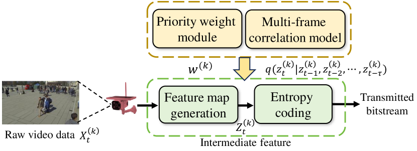
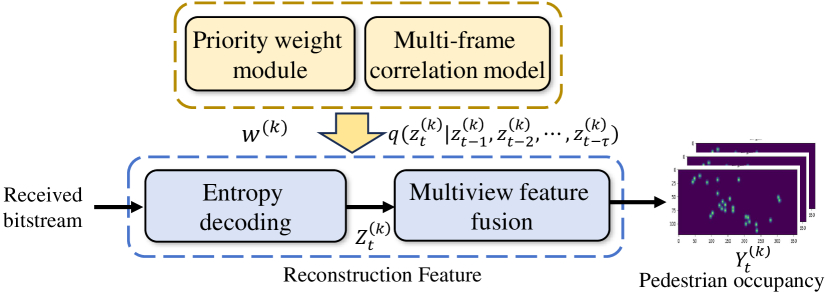
In this subsection, we outline the workflow of our PIB framework, designed for collaborative edge video analytics. As depicted in Fig. 4, the process starts with each edge camera (denoted by ) capturing raw video data and extracting feature maps. These cameras utilize priority weights to optimize the balance between communication costs and perception accuracy, adapting to varying channel conditions. The extracted features are then compressed using entropy coding and sent as a bitstream to the edge server for further processing. On the server (see Fig. 4), the video features are reconstructed using the shared parameters such as weights and the variational model parameters . The server integrates these multi-view features to estimate , such as pedestrian occupancy and object detection. This approach leverages historical frame correlations through a multi-frame correlation model to enhance prediction accuracy.
IV-B Variational Approximation Method
The objective function of information bottleneck in Eq. (7) can be divided into two parts. The first part is , which denotes the quality of video reconstruction by decoding at an edge server. The second part is , which denotes the compression efficiency for feature extraction. As it has been shown in the way a decoder works, can be any valid type of conditional distributions, but most often it is not feasible enough for straightforward calculation. Because of this complexity, it is highly challenging to directly compute the two mutual information components in Eq. (7).
As for the first part, we adopt the variational approach[50]. This approach suggests that the decoder is part of a simpler group of distributions called . We then search for a distribution within this group that is most similar to the best possible decoder distribution, using the KL-divergence to measure the closeness. is a learnable parameter. Because computing the high-dimensional integrals in the posterior is infeasible, we substitute the optimal inference model with a variational approximation. Thus, we obtain the lower bound of , as established in Proposition 1.
Proposition 1:
The probabilistic model of decoder maps a representation into task inference . Let denote the variational approximation of decoder . We can obtain
| (12) |
Proof:
We start with the standard definition of mutual information:
| (13) |
which utilizes the relationship to express the mutual information in terms of the ratio of the conditional probability to the marginal probability of .
Introducing the Kullback-Leibler (KL) divergence, which measures how the distribution approximates the true distribution , we have:
| (14) |
where the KL divergence is always non-negative. This leads to:
| (15) |
which can be simplified to:
| (16) |
Therefore, we can derive the lower bound for the mutual information as follows:
| (17) | ||||
where is the entropy of , a constant that reflects the inherent uncertainty in independent of .
To establish an upper bound for the term in the context of the complexity in directly minimizing it, we proceed as follows. Recognizing that from the properties of entropy, we obtain the inequality:
| (18) | ||||
where we use the latent variables as the side information to encode the quantized feature and we have used . The joint entropy represents the communication cost, which is minimized when the joint entropy is minimized.
Proposition 2:
The upper bound for the mutual information term in Eq. 7 is given by:
| (19) | ||||
where is the variational distribution conditioned on the latent variables with parameters , and is the marginal variational distribution with parameters .
Proof:
The proof begins by recognizing that the joint entropy represents the communication cost, which is minimized when the joint entropy is minimized. The joint entropy can be expressed as the expectation over the logarithm of the ratio of the true joint distribution to the variational distribution , where represents the learnable parameter:
| (20) | ||||
where is the KL-divergence between the distribution of and . The KL-divergence is non-negative, thus we have:
| (21) |
Combining the joint entropy equation (20) with inequality (21), we get:
| (22) | ||||
Thus, we can substitute Ineq. (21) into Ineq. (LABEL:eq:hz) to obtain the result in Ineq. (19).
It should be noted that the lower bound in Ineq. (17) and upper bound in Ineq. (19) enables us to establish an upper limit on the objective function in minimization problem in (7). This makes it easier to minimize with the corresponding loss function during network training, as discussed in Sec. IV-D.
IV-C Multi-Frame Correlation Model
Inspired by the previous work [12], PIB framework utilizes a multi-frame correlation model to leverage variational approximation to capture the temporal dynamics in video sequences. This approach utilizes the temporal redundancy across contiguous frames to model the conditional probability distribution effectively. Our model approximates the next feature in the sequence by considering the variational distribution , which can be modeled as a Gaussian distribution aimed at mimicking the true conditional distribution of the subsequent frame given the previous frames:
where and are parametric functions of the preceding frames, encapsulating the temporal dependencies. These functions are modeled using a deep neural network with parameters learned from data. By optimizing the variational parameters, our model aims to closely match the true distribution, thus encoding the features more efficiently.
IV-D Network Loss Functions Derivation
In this subsection, we formulate our network loss functions to enhance the information transmission in a multi-camera scenario based on the priority-driven mechanism and the IB principle as discussed in Sec. II-B and Sec. III-A.
Given the variability in channel quality and the occurrence of delays, we introduce the first loss function, , designed to minimize the impact of unreliable data sources while maximizing inference accuracy. We also consider to improve the number of perceived moving objects (). Thus, the loss function of the MLP network in Sec. II-B is:
| (23) |
where denotes a permissible delay that cannot result in errors in multi-view fusion, and represents the target weight for a camera without excessive delay. The second loss function aims to minimize the upper bound of the mutual information, following the inequalities derived in (17) and (19). ensures efficient encoding while preserving essential information for accurate prediction:
| (24) | ||||
The first term of ignores in Ineq. (12) because it is a constant. represents the penalty for the excessive communication cost of the variation approximation , which captures the degradation of training decoder . In Sec. IV-C, the Multi-Frame Correlation Model leverages temporal dynamics, which is critical for sequential data processing in video analytics. The third loss function, , is needed to minimize the KL divergence between the true distribution of frame sequences and the modeled variational distribution:
| (25) |
where . These loss functions collectively aim to optimize the trade-off between data transmission costs and perceptual accuracy, crucial for enhancing the performance of edge analytics in multi-camera systems. Alg. 1 introduces the detailed procedure of feature extraction and variational approximation.
IV-E Gate Mechanism Based on Distributed Online Learning
The gate mechanism based on distributed online learning is designed to solve the combinatorial multi-armed bandit (CMAB) problem (11) formulated in Sec. III-B. In this subsection, we first introduce the intuitive ideas of gate mechanism. Then, we provide the details and explanation of the pseudocode. Finally, the evaluation of regret performance and communication cost for distributed execution is analyzed mathematically.
IV-E1 Distributed Online Learning for CMAB Problem
Firstly, we propose a distributed Upper Confidence Bound (UCB) algorithm to address this problem, leveraging the independence of each camera agent to learn the optimal transmission strategy. This approach is particularly effective for managing the dynamic nature of the multi-camera network, where real-time channel quality and server load can significantly impact the overall system performance. Specifically, we assume that each arm represents the connection establishment between a camera and an edge server. The super arm is the combination of these connections. The reward is defined based on the gain in MODA by adding the -th camera’s feature to the ego camera in Eq. (9).
The intuitive idea behind using distributed UCB is to manage dynamic CSI and ROI efficiently. Each camera agent independently explores and exploits available edge servers based on local observations, making the system robust to changing network conditions. The algorithm has two phases: exploration and exploitation. In the exploration phase, each agent gathers information on potential rewards. In the exploitation phase, the agent selects the best action based on the UCB value, balancing exploration and exploitation under uncertainty. The UCB value for edge server at time is , where is the estimated reward, driving exploitation. The second term () accounts for uncertainty, encouraging exploration[51]. The key intuition is that actions that have been selected fewer times carry more uncertainty, so they are given a higher bonus to encourage exploration. Conversely, as an action is selected more often and its reward estimate becomes more reliable, the bonus decreases, leading to more exploitation of that action. The parameter balances how aggressively the algorithm explores uncertain actions versus exploiting known rewards. The square root component diminishes as more information is gathered, while the logarithmic term ensures the exploration bonus decreases slowly, encouraging exploration of less frequently chosen actions. Alg. 2 provides the pseudocode for the proposed gate mechanism with distributed online learning.
As for distributed execution of Alg. 2, each camera agent independently updates its channel state and edge server load based on local observations (Line 7). This allows each agent to learn the optimal transmission strategy without centralized control. Moreover, each agent computes the UCB value for each edge server and selects the action that maximizes the UCB value (Lines 9-11). This decentralized decision-making process ensures scalability and adaptability in dynamic environments. To ensure consistency across agents, periodic communication rounds are initiated (Line 19). During these rounds, each agent shares its local reward estimates and action counts with a designated central edge server. This central server aggregates the information and updates the global estimates, which are then shared with all agents (Lines 19-24). This step maintains synchronization across the distributed network without requiring continuous centralized control.
IV-E2 Regret Analysis
The regret analysis reflects the efficiency and adaptability of the algorithm in optimizing network performance. A lower regret bound indicates that the algorithm performs close to the optimal strategy, ensuring high inference accuracy and efficient resource utilization despite the dynamic environment and varying network conditions. In the context of a multi-camera sensing network, the choices between different cameras and edge servers are interdependent. Furthermore, the connections between different cameras and edge servers exhibit heterogeneity, with each super arm having different distribution parameters. Therefore, we consider a CMAB problem with a non-i.i.d. assumption and derive its regret upper bound in the following part.
The regret is an important metric to evaluate the performance of online learning algorithm. The regret over a time horizon is defined as the difference between the maximum expected reward obtainable by an optimal strategy and the expected reward obtained by the algorithm:
| (26) |
where represents an action, and is the expected reward for action . To derive the regret bounds, we first establish a lemma using Bernstein’s inequality in Lemma 1.
Lemma 1:
(Bernstein’s inequality) Let be independent random variables such that almost surely. Then, for any ,
| (27) |
Theorem 1:
In a dynamic environment where the reward variance is denoted as , the cumulative regret over of the distributed UCB algorithm with non-i.i.d rewards is bounded by:
| (28) |
where represents the maximum number of arms in the optimal super arm, is the standard deviation of the reward, and is an upper bound on the linear growth rate of the number of times UCB algorithm arms are selected over time555It indicates that follows a linear growth trend, i.e., ..
Proof:
We start by defining the reward for camera transmitting to edge server at time as . The mean reward for this transmission is denoted by , and the variance of the reward is . The total variance in rewards across all camera-edge server pairs is represented by , which accounts for variability due to both the dynamic channel state information (CSI) and the edge server load fluctuations. To derive the regret bound, we use Bernstein’s inequality to bound the sum of rewards for each camera-edge server pair. For any , Bernstein’s inequality gives the following probability bound:
| (29) |
Now, we set as to account for the cumulative uncertainty over time . Substituting this into the right-hand side of Bernstein’s inequality, we get:
As increases, the dominant terms in the expression are in both the numerator and the denominator. Therefore, we approximate the right-hand side as:
| (30) |
Thus, combining Ineq. (29) and Eq. (30), we obtain:
| (31) |
It implies that, with high probability, when is sufficiently large, we have:
| (32) |
Therefore, the regret for each camera-edge server pair, denoted by arm , can be bounded as:
| (33) |
where represents the regret due to not always selecting the optimal arm , while the term captures the uncertainty in reward estimation. Since the UCB algorithm selects the arm that maximizes the UCB value, we have:
| (34) |
where is the number of times the camera-edge server pair has been selected up to time . This implies that:
| (35) |
Therefore, the upper bound on the cumulative loss (i.e., regret) for arm can be expressed as:
| (36) |
Since is an unbiased estimate of , its expected value is zero. Thus, the regret is mainly determined by the term . We approximate the cumulative sum of this term by using an integral, given that is assumed to grow linearly with time, i.e., , where is a constant. Under this assumption, we have:
| (37) |
Thus, the regret for a single arm can be bounded as:
| (38) |
To obtain the total regret , we sum the regret over all camera-edge server pairs in the set of arms :
| (39) |
Then, we sum the bias and variance terms across all arms. For the bias term, we have:
| (40) |
where is the number of arms in the optimal super arm, and is the maximum variance among all arms. Therefore, when is sufficiently large, the overall regret bound can be expressed as Thus, the cumulative regret for the distributed UCB algorithm is bounded by the sum of the regret from all camera-edge server pairs, ensuring that the regret grows sub-linearly with respect to .
Proposition 3:
It is assumed that there are camera agents and time steps. The computational complexity of the proposed DOL method in Alg. 2 for each camera agent at each time step is . The overall time complexity is .
Proof:
Each camera agent computes the UCB value for each edge server at each time step . This involves updating the channel state and edge server load, computing the UCB values, selecting the optimal action, and updating the reward estimates. As for each camera agent, the complexity of updating the channel state and edge server load for each camera agent is . Moreover, the complexity of computing the UCB value for each edge server is . The complexity of selecting the action that maximizes the UCB value is . Thus, the complexity for each camera agent at each time step is . Given that there are camera agents and time steps, the overall time complexity is .
Proposition 4:
Assuming there are communication rounds over time steps, the total communication cost of Alg. 2 is .
Proof:
Each communication round involves local communication between each camera agent and the central edge server, as well as the global aggregation and update phases. 1) Local Communication: Each camera agent communicates its local reward estimates and action counts for each edge server to the central edge server. The communication cost for each agent per round is . Given agents, the total local communication cost per round is . 2) Global Aggregation: The central edge server aggregates the information from all camera agents. The complexity of aggregating the information is . 3) Global Update: The central server then broadcasts the updated global reward estimates to all agents. The communication cost for broadcasting is . Assuming there are communication rounds over time steps, the total communication cost is .
V Performance Evaluation
V-A Simulation Setup
We set up simulations to evaluate our PIB framework, aiming at predicting pedestrian occupancy in urban settings using multiple cameras. These simulations replicate a city environment, with variables like signal frequency and device density affecting the outcomes.
Our simulations use a 2.4 GHz operating frequency, a path loss exponent of 3.5, and a shadowing deviation of 8 dB. Devices emit an interference power of 0.1 Watts, with densities ranging from 10 to 100 devices per 100 square meters, allowing us to test different levels of congestion. The bandwidth is set to 2 MHz, with cameras located at about 200 meters from the edge server. We employ the Wildtrack dataset from EPFL, which features high-resolution images from seven cameras located in a public area, capturing unscripted pedestrian movements[53]. This dataset provides 400 frames per camera at 2 frames per second, documenting over 40,000 bounding boxes that highlight individual movements across more than 300 pedestrians. Our code will be available at github.com/fangzr/PIB-Prioritized-Information-Bottleneck-Framework.
The primary measure we use is MODA, which assesses the system’s ability to accurately detect pedestrians based on missed and false detections. We also look at the rate-performance tradeoff to understand how communication overhead affects system performance. For comparative analysis, we consider five baselines, including video coding and image coding:
-
•
TOCOM-TEM[12]: A task-oriented communication framework utilizing a temporal entropy model for edge video analytics. It employs the deterministic Information Bottleneck principle to extract and transmit compact, task-relevant features, integrating spatial-temporal data on the server for improved inference accuracy.
-
•
JPEG[54]: A widely used image compression standard employing lossy compression algorithms to reduce image data size, commonly used to decrease communication load in networked camera systems.
-
•
H.265[55]: Also known as High Efficiency Video Coding (HEVC) or MPEG-H Part 2, which offers up to 50% better data compression than its predecessor H.264 (MPEG-4 Part 10), while maintaining the same video quality, crucial for efficient data transmission in high-density camera networks.
-
•
H.264[56]: Known as Advanced Video Coding (AVC) or MPEG-4 Part 10, which significantly enhances video compression efficiency, allowing high-quality video transmission at lower bit rates.
-
•
AV1[57]: AOMedia Video 1 (AV1) is an open, royalty-free video coding format developed by the Alliance for Open Media (AOMedia), designed to succeed VP9 with improved compression efficiency. AV1 outperforms existing codecs like H.264 and H.265, making it ideal for online video applications.
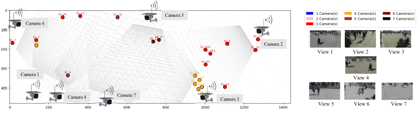
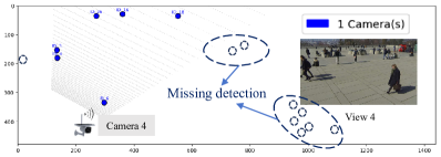
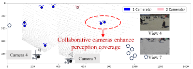
In the simulation study, we examine the effectiveness of multiple camera systems in forecasting pedestrian presence. Unlike a single-camera configuration, this method minimizes obstructions commonly found in crowded locations by integrating perspectives from various angles. Fig. 5 demonstrates our experimental setup, where seven wireless edge cameras jointly perceive a 12m×36m area quantized into a 480×1440 grid using a resolution of 2.5 . We use contour lines to display the camera’s perception range and the resolution of coordinates within that range. The denser the lines, the closer the perceived target is to the camera, and the higher the perception accuracy. Additionally, to clearly show the coverage of pedestrians at different positions by edge cameras, different colors represent the number of cameras covering each pedestrian. It can be observed that pedestrians in different locations have different probabilities of being detected, which will also affect the priority selection of cameras. Fig. 6(a) shows the perception results using a single camera (the 4th edge camera). The dashed circles represent pedestrians that are missing detection. It is evident that the perception range of a single camera is limited to its own angle and coverage area, resulting in numerous missing detections. In Fig. 6(b), we let the 4th and 7th edge cameras collaborate with each other. It can be observed that the collaboration enhances perception coverage, though there are still several pedestrians not detected compared to the results from seven edge cameras. This highlights the improved but still limited capability of collaborative perception with only two cameras, indicating the necessity for a higher number of cameras to achieve comprehensive coverage and accurate pedestrian detection666Our demo is available at the url: github.com/fangzr/PIB-Prioritized-Information-Bottleneck-Framework.
Nevertheless, the benefit of collaborative perception is accompanied by excessive communication overhead. The communication bottleneck refers to network capacity constraints that prevent real-time data transmission, causing frame latency. This issue is prevalent in UDP-based wireless streaming systems, where high throughput often results in out-of-order or delayed frames due to varying channel quality and jitter. Moreover, different coding schemes cause varying delays in dynamic channel conditions, misaligning data fusion due to channel quality and jitter. Therefore, in order to evaluate how latency differences affect perception accuracy, we set communication bottleneck constraints. In our experiments, we use MODA (Multiple Object Detection Accuracy) and MODP (Multiple Object Detection Precision) to assess coding efficiency and robustness.
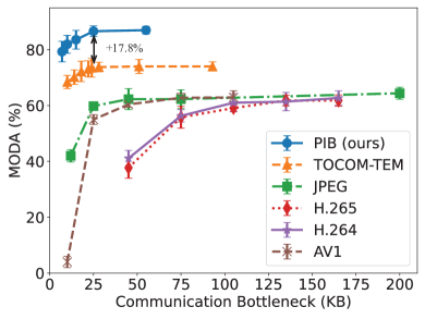
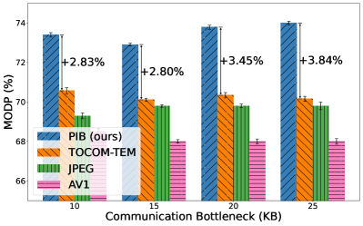
In Fig. 7, PIB exhibits higher MODA across different communication bottlenecks compared to five baselines by more than 17.8%. This is due to PIB’s strategic multi-view feature fusion, informed by channel quality and priority-based ROI selection. PIB prioritizes the shared information to mitigate delays that could degrade multi-camera perception accuracy. Interestingly, JPEG outperforms video coding schemes like H.265 and AV1 in our experiments, due to the low FPS of 2 used for video transmission, which does not leverage motion prediction advantages. AV1 performs well due to its high compression efficiency compared to H.264 and H.265. Fig. 8 shows that PIB achieves higher MODP performance compared to three other baselines. The results indicate that MODP is less affected by latency because it measures the precision of detection without considering missed detections, whereas MODA is more impacted as it accounts for both missed and false detections.
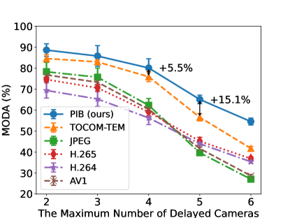
Fig. 9 depicts the performance rates of different compression techniques in a multi-view scenario in terms of the number of delayed cameras. Our proposed PIB method and TOCOM-TEM, both utilizing multi-frame correlation models, effectively reduce redundancy across multiple frames, achieving superior MODA at equivalent compression rates. PIB, in particular, employs a prioritized IB framework, enabling an adaptive balance between compression rate and collaborative sensing accuracy, optimizing MODA across various channel conditions. It is worth noting that the impact on collaborative perception MODA can be ignored in scenarios with fewer delayed cameras (<3). However, as channel conditions worsen and more cameras experience frame delays due to failing to meet communication bottleneck constraints, the performance significantly degrades.
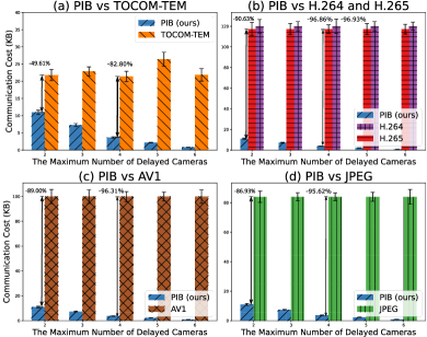
In Fig. 10, we analyze the impact of the number of delayed cameras on the communication cost777The communication cost of a method is the average size of each frame. The instantaneous streaming rate is equal to the communication cost multiplied by the frames per second (fps). for various algorithms. The PIB algorithm demonstrates a significant reduction in communication costs as the number of delayed cameras increases. When the number of delayed cameras equals 4, PIB, utilizing a gate mechanism based on a distributed UCB algorithm, effectively filters out useless streaming data, greatly reducing communication costs. Compared to TOCOM-TEM, PIB achieves an impressive 82.8% decrease in communication costs. This efficiency is due to the algorithm’s priority mechanism, which adeptly assigns weights and filters out adverse information caused by delays. Consequently, PIB prioritizes the transmission of high-quality features from cameras with more accurate occupancy predictions. For a fair comparison, baselines are selected at their highest MODA with the minimum communication cost data. Due to the use of an information bottleneck framework, PIB extracts only task-related features, resulting in a significantly reduced compression rate compared to five compression baselines.
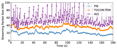
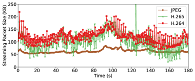
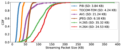
Fig. 11(a) shows the streaming packet size for PIB, TOCOM-TEM, and AV1 over a period of 3 minutes. For a fair comparison, all coding methods are selected at their highest MODA with the minimum communication cost data. PIB has the smallest streaming packet size among the three methods. Additionally, both PIB and TOCOM-TEM exhibit less fluctuation in packet size compared to AV1, ensuring better transmission robustness under poor channel conditions. Fig. 11(b) reflects that JPEG compression results in smaller and less fluctuating streaming packet sizes compared to H.264 and H.265. This is because the raw data transmission rate is only 2 fps, limiting the efficiency of video compression codecs. Fig. 11(c) illustrates the CDF of streaming packet sizes for all algorithms. The Standard Deviation (SD) of each algorithm is also calculated by . The advantage of smaller SD is to improve transmission robustness, particularly in environments with poor channel conditions, as it leads to less jitter and requires smaller buffer sizes. As shown in Fig. 11(c), PIB has the smallest SD (3.84 KB), indicating the least fluctuation in packet sizes. This is followed by TOCOM-TEM (4.24 KB) and JPEG (6.18 KB). Moreover, five baselines exhibit higher SD values. Therefore, PIB not only significantly reduces the streaming transmission requirements but also has a smaller SD, indicating more consistent packet sizes.
| Number | Comm. Cost | MODA (%) | MODP (%) |
| 1 | 2.19 KB | 65.11 (+17.99%) | 71.53 (+2.59%) |
| 2 | 3.68 KB | 78.09 (+19.93%) | 72.71 (+1.65%) |
| 3 | 7.29 KB | 84.99 (+8.85%) | 72.92 (+0.29%) |
| 4 | 10.98 KB | 88.03 (+3.57%) | 74.23 (+1.80%) |
| 5 | 15.84 KB | 88.64 (+0.69%) | 75.15 (+1.24%) |
| 6 | 17.68 KB | 88.76 (+0.14%) | 75.80 (+0.87%) |
| No Fusion | 0.82 KB | 55.17 | 69.72 |
Our priority-based mechanism selects the camera with the most targets within the RRoI as the highest transmission priority on the channel. Consequently, the collaboration priority is determined by the number of targets in each camera’s perception area. As shown in Table I, a mere 0.82 KB of perception data can achieve a MODA accuracy of up to 55.17% and a MODP accuracy of 69.72%. This indicates a significant redundancy among the perception data acquired from multiple edge cameras. As the number of collaborative cameras increases, the communication cost sent to the edge server also increases. Initially, with the addition of more cameras, the perception performance improves significantly. However, the performance gain from further collaboration gradually diminishes, demonstrating the principle of diminishing marginal returns.
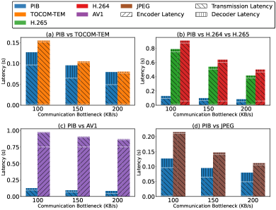
In Fig. 12, the communication bottleneck versus latency for different algorithms is shown. Although PIB increases the decoding complexity compared to TOCOM-TEM and JPEG, it significantly reduces redundant data transmission by employing a priority information bottleneck framework that selects cameras with the most prediction-relevant information. Additionally, the distributed online learning UCB algorithm filters out useless data. Consequently, PIB demonstrates higher compression efficiency compared to various video coding methods. Notably, PIB’s encoder latency is only 0.27% of that of the widely adopted AV1 compression codec.
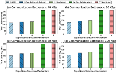
Fig. 13 demonstrates the effectiveness of the proposed Gate Mechanism Based on Distributed Online Learning (Sec. IV-E). This figure evaluates total latency, defined as the sum of inference, relay, and transmission latency, excluding encoder latency, under different communication bottlenecks for various edge node selection mechanisms. Four baselines are used: Avg-Bottleneck-Optimal (exhaustive search for highest average bottleneck), Stochastic (random selection of relay and fusion nodes), Non-Collaboration (single edge server for fusion), and Non-Relay (lowest load edge server). The UCB method consistently achieves the lowest total latency, adapting efficiently to edge server load and channel conditions with minimal overhead, thereby optimizing collaborative selection of edge servers. Fig. 14 illustrates the impact of different numbers of edge servers on the latency of multi-camera collaborative sensing data transmission and inference under varying communication bottlenecks. The results indicate that as the number of edge servers increases, the overall average latency of the cameras significantly decreases. This is because the communication bottleneck is comparable in magnitude to the size of the intermediate representations transmitted by the cameras. Therefore, increasing the number of edge servers markedly reduces latency, showcasing the effectiveness of adding more edge servers in enhancing system performance.

VI Conclusion
In this paper, we have proposed the Prioritized Information Bottleneck (PIB) framework as a robust solution for collaborative edge video analytics. Our contributions are two-fold. First, we have developed a prioritized inference mechanism to intelligently determine the importance of different camera’ FOVs, effectively addressing the constraints imposed by channel capacity and data redundancy. Second, the PIB framework showcases its effectiveness by notably decreasing communication overhead and improving tracking accuracy without requiring video reconstruction at the edge server. Extensive numerical results show that: PIB not only surpasses the performance of conventional methods like TOCOM-TEM, JPEG, H.264, H.265, and AV1 with a marked improvement of up to 17.8% in MODA but also achieves a considerable reduction in communication costs by 82.80%, while retaining low latency and high-quality multi-view sensory data processing under less favorable channel conditions.
References
- [1] Z. Fang, S. Hu, L. Yang, Y. Deng, X. Chen, and Y. Fang, “PIB: Prioritized information bottleneck framework for collaborative edge video analytics,” in IEEE Global Communications Conference (GLOBECOM), Cape Town, South Africa, Dec. 2024, pp. 1–6.
- [2] A. Padmanabhan, N. Agarwal, A. Iyer, G. Ananthanarayanan, Y. Shu, N. Karianakis, G. H. Xu, and R. Netravali, “Gemel: Model merging for memory-efficient, real-time video analytics at the edge,” in 20th USENIX Symposium on Networked Systems Design and Implementation (NSDI 23), Boston, MA, 2023, pp. 973–994.
- [3] X. Dai, P. Yang, X. Zhang, Z. Dai, and L. Yu, “Respire: Reducing spatial–temporal redundancy for efficient edge-based industrial video analytics,” IEEE Transactions on Industrial Informatics, vol. 18, no. 12, pp. 9324–9334, Mar. 2022.
- [4] H. Wang, J. Huang, G. Wang, H. Lu, and W. Wang, “Contactless patient care using hospital IoT: CCTV camera based physiological monitoring in ICU,” IEEE Internet of Things Journal, vol. 11, no. 4, pp. 5781–5797, Aug. 2023.
- [5] X. Yu, Z. Ying, N. Birkbeck, Y. Wang, B. Adsumilli, and A. C. Bovik, “Subjective and objective analysis of streamed gaming videos,” IEEE Transactions on Games, pp. 1–14, 2023.
- [6] G. Pan, H. Zhang, S. Xu, S. Zhang, and X. Chen, “Joint optimization of video-based AI inference tasks in MEC-assisted augmented reality systems,” IEEE Transactions on Cognitive Communications and Networking, vol. 9, no. 2, pp. 479–493, 2023.
- [7] T. Kämäräinen, M. Siekkinen, A. Ylä-Jääski, W. Zhang, and P. Hui, “A measurement study on achieving imperceptible latency in mobile cloud gaming,” in Proceedings of the 8th ACM on Multimedia Systems Conference, Taipei, Taiwan, Jun. 2017, pp. 88–99.
- [8] M. Xu, W. C. Ng, W. Y. B. Lim, J. Kang, Z. Xiong, D. Niyato, Q. Yang, X. Shen, and C. Miao, “A full dive into realizing the edge-enabled metaverse: Visions, enabling technologies, and challenges,” IEEE Communications Surveys & Tutorials, vol. 25, no. 1, pp. 656–700, Nov. 2023.
- [9] L. Corneo, N. Mohan, A. Zavodovski, W. Wong, C. Rohner, P. Gunningberg, and J. Kangasharju, “(How much) can edge computing change network latency?” in IFIP Networking Conference (IFIP Networking). Espoo and Helsinki, Finland: IEEE, Jun. 2021, pp. 1–9.
- [10] L. Marelli and G. Testa, “Scrutinizing the EU general data protection regulation,” Science, vol. 360, no. 6388, pp. 496–498, May 2018.
- [11] Ponemon Institute, “New ponemon institute study finds 60% of it and security leaders are not confident in their ability to secure access to cloud environments,” 2021, online Accessed: 2022-07-20.
- [12] J. Shao, X. Zhang, and J. Zhang, “Task-oriented communication for edge video analytics,” IEEE Transactions on Wireless Communications, vol. 23, no. 5, pp. 4141–4154, May 2024.
- [13] M. Al-Qizwini, I. Barjasteh, H. Al-Qassab, and H. Radha, “Deep learning algorithm for autonomous driving using GoogleNet,” in IEEE Intelligent Vehicles Symposium (IV), Los Angeles, CA, Jun. 2017, pp. 89–96.
- [14] K. Gao, H. Wang, H. Lv, and W. Liu, “Localization-oriented digital twinning in 6G: A new indoor-positioning paradigm and proof-of-concept,” IEEE Transactions on Wireless Communications, 2024.
- [15] A. Yaqoob, T. Bi, and G.-M. Muntean, “A survey on adaptive 360 video streaming: Solutions, challenges and opportunities,” IEEE Communications Surveys & Tutorials, vol. 22, no. 4, pp. 2801–2838, 2020.
- [16] Y. Cui, G. Jiang, M. Yu, Y. Chen, and Y.-S. Ho, “Stitched wide field of view light field image quality assessment: Benchmark database and objective metric,” IEEE Transactions on Multimedia, vol. 26, pp. 5092–5107, Nov. 2023.
- [17] Z. Jiang, X. Zhang, Y. Xu, Z. Ma, J. Sun, and Y. Zhang, “Reinforcement learning based rate adaptation for 360-degree video streaming,” IEEE Transactions on Broadcasting, vol. 67, no. 2, pp. 409–423, Oct. 2020.
- [18] Z. Fang, S. Hu, H. An, Y. Zhang, J. Wang, H. Cao, X. Chen, and Y. Fang, “PACP: Priority-aware collaborative perception for connected and autonomous vehicles,” IEEE Transaction of Mobile Computing (Accepted), Aug. 2024.
- [19] X. Chen, Y. Deng, H. Ding, G. Qu, H. Zhang, P. Li, and Y. Fang, “Vehicle as a service (VaaS): Leverage vehicles to build service networks and capabilities for smart cities,” IEEE Communications Surveys & Tutorials, (DOI: 10.1109/COMST.2024.3370169), 2024.
- [20] S. Hu, Z. Fang, H. An, G. Xu, Y. Zhou, X. Chen, and Y. Fang, “Adaptive communications in collaborative perception with domain alignment for autonomous driving,” arXiv preprint arXiv:2310.00013, 2023.
- [21] S. Hu, Z. Fang, X. Chen, Y. Fang, and S. Kwong, “Towards full-scene domain generalization in multi-agent collaborative bird’s eye view segmentation for connected and autonomous driving,” 2024.
- [22] S. Hu, Z. Fang, Z. Fang, Y. Deng, X. Chen, and Y. Fang, “Agentscodriver: Large language model empowered collaborative driving with lifelong learning,” 2024.
- [23] S. Hu, Z. Fang, Y. Deng, X. Chen, and Y. Fang, “Collaborative perception for connected and autonomous driving: Challenges, possible solutions and opportunities,” arXiv preprint arXiv:2401.01544, 2024.
- [24] X. Chi, H. Chen, G. Li, Z. Ni, N. Jiang, and F. Xia, “EDSP-Edge: Efficient dynamic edge service entity placement for mobile virtual reality systems,” IEEE Transactions on Wireless Communications, vol. 23, no. 4, pp. 2771–2783, Aug. 2024.
- [25] Y. Jin, J. Liu, F. Wang, and S. Cui, “Ebublio: Edge-assisted multiuser 360° video streaming,” IEEE Internet of Things Journal, vol. 10, no. 17, pp. 15 408–15 419, Apr. 2023.
- [26] R. Tu, G. Jiang, M. Yu, Y. Zhang, T. Luo, and Z. Zhu, “Pseudo-reference point cloud quality measurement based on joint 2-D and 3-D distortion description,” IEEE Transactions on Instrumentation and Measurement, vol. 72, pp. 1–14, Jun. 2023.
- [27] D. Wu, D. Zhang, M. Zhang, R. Zhang, F. Wang, and S. Cui, “ILCAS: Imitation learning-based configuration-adaptive streaming for live video analytics with cross-camera collaboration,” IEEE Transactions on Mobile Computing, vol. 23, no. 6, pp. 6743–6757, Jun. 2024.
- [28] Y.-F. Lu, J.-W. Gao, Q. Yu, Y. Li, Y.-S. Lv, and H. Qiao, “A cross-scale and illumination invariance-based model for robust object detection in traffic surveillance scenarios,” IEEE Transactions on Intelligent Transportation Systems, vol. 24, no. 7, pp. 6989–6999, Apr. 2023.
- [29] Z. Bao, S. Yang, Z. Huang, M. Zhou, and Y. Chen, “A lightweight block with information flow enhancement for convolutional neural networks,” IEEE Transactions on Circuits and Systems for Video Technology, vol. 33, no. 8, pp. 3570–3584, Aug. 2023.
- [30] R. Lu, Z. Cheng, B. Chen, and X. Yuan, “Motion-aware dynamic graph neural network for video compressive sensing,” IEEE Transactions on Pattern Analysis and Machine Intelligence, (DOI: 10.1109/TPAMI.2024.3395804), pp. 1–17, May 2024.
- [31] M. Xu, H. Du, D. Niyato, J. Kang, Z. Xiong, S. Mao, Z. Han, A. Jamalipour, D. I. Kim, X. Shen, V. C. M. Leung, and H. V. Poor, “Unleashing the power of edge-cloud generative ai in mobile networks: A survey of AIGC services,” IEEE Communications Surveys & Tutorials, vol. 26, no. 2, pp. 1127–1170, Jan. 2024.
- [32] T. Li, J. Sun, Y. Liu, X. Zhang, D. Zhu, Z. Guo, and L. Geng, “ESMO: Joint frame scheduling and model caching for edge video analytics,” IEEE Transactions on Parallel and Distributed Systems, vol. 34, no. 8, pp. 2295–2310, May 2023.
- [33] M. Khani, G. Ananthanarayanan, K. Hsieh, J. Jiang, R. Netravali, Y. Shu, M. Alizadeh, and V. Bahl, “RECL: Responsive resource-efficient continuous learning for video analytics,” in 20th USENIX Symposium on Networked Systems Design and Implementation (NSDI 23), 2023, pp. 917–932.
- [34] S. Wang, S. Bi, and Y.-J. A. Zhang, “Edge video analytics with adaptive information gathering: A deep reinforcement learning approach,” IEEE Transactions on Wireless Communications, vol. 22, no. 9, pp. 5800–5813, Jan. 2023.
- [35] P. Zhang, W. Xu, Y. Liu, X. Qin, K. Niu, S. Cui, G. Shi, Z. Qin, X. Xu, F. Wang, Y. Meng, C. Dong, J. Dai, Q. Yang, Y. Sun, D. Gao, H. Gao, S. Han, and X. Song, “Intellicise wireless networks from semantic communications: A survey, research issues, and challenges,” IEEE Communications Surveys & Tutorials (DOI: 10.1109/COMST.2024.3443193), Aug. 2024.
- [36] Y. Shao, Q. Cao, and D. Gündüz, “A theory of semantic communication,” IEEE Transactions on Mobile Computing (DOI: 10.1109/TMC.2024.3406375), pp. 1–18, May 2024.
- [37] H. Xie, Z. Qin, and G. Y. Li, “Semantic communication with memory,” IEEE Journal on Selected Areas in Communications, vol. 41, no. 8, pp. 2658–2669, Jun. 2023.
- [38] S. Zhou, D. Van Le, R. Tan, J. Q. Yang, and D. Ho, “Configuration-adaptive wireless visual sensing system with deep reinforcement learning,” IEEE Transactions on Mobile Computing, vol. 22, no. 9, pp. 5078–5091, May 2023.
- [39] Y. Chen, S. Zhang, Y. Jin, Z. Qian, M. Xiao, W. Li, Y. Liang, and S. Lu, “Crowdsourcing upon learning: Energy-aware dispatch with guarantee for video analytics,” IEEE Transactions on Mobile Computing, vol. 23, no. 4, pp. 3138–3155, 2024.
- [40] S. Hu, Z. Lou, X. Yan, and Y. Ye, “A survey on information bottleneck,” IEEE Transactions on Pattern Analysis and Machine Intelligence, (DOI: 10.1109/TPAMI.2024.3366349), pp. 1–20, Feb. 2024.
- [41] A. Pensia, V. Jog, and P.-L. Loh, “Extracting robust and accurate features via a robust information bottleneck,” IEEE Journal on Selected Areas in Information Theory, vol. 1, no. 1, pp. 131–144, May 2020.
- [42] S. Wang, C. Li, Y. Li, Y. Yuan, and G. Wang, “Self-supervised information bottleneck for deep multi-view subspace clustering,” IEEE Transactions on Image Processing, vol. 32, pp. 1555–1567, Feb. 2023.
- [43] R. Wang, X. He, R. Yu, W. Qiu, B. An, and Z. Rabinovich, “Learning efficient multi-agent communication: An information bottleneck approach,” in International Conference on Machine Learning (ICML), Virtual Event, 2020, pp. 9908–9918.
- [44] D. Kim, S. Moon, D. Hostallero, W. Kang, T. Lee, K. Son, and Y. Yi, “Learning to schedule communication in multi-agent reinforcement learning,” arXiv preprint arXiv:1902.01554, 2019.
- [45] Y. Du, B. Liu, V. Moens, Z. Liu, Z. Ren, J. Wang, and H. Zhang, “Learning correlated communication topology in multi-agent reinforcement learning,” in Proceedings of the 20th International Conference on Autonomous Agents and MultiAgent Systems (AAMAS), London, United Kingdom, May, 2021, pp. 456–464.
- [46] Y. Liu, W. Wang, Y. Hu, J. Hao, X. Chen, and Y. Gao, “Multi-agent game abstraction via graph attention neural network,” in Proceedings of the Thirty-Fourth AAAI Conference on Artificial Intelligence (AAAI), New York, NY, February, 2020, pp. 7211–7218.
- [47] Y. Niu, R. R. Paleja, and M. C. Gombolay, “Multi-agent graph-attention communication and teaming,” in Proceedings of the 20th International Conference on Autonomous Agents and MultiAgent Systems (AAMAS), London, United Kingdom, May, 2021, pp. 964–973.
- [48] Y.-C. Liu, J. Tian, N. Glaser, and Z. Kira, “When2com: Multi-agent perception via communication graph grouping,” in IEEE/CVF Conference on Computer Vision and Pattern Recognition (CVPR), Seattle, WA (Virtual), 2020, pp. 4106–4115.
- [49] N. Tishby, F. C. Pereira, and W. Bialek, “The information bottleneck method,” arXiv preprint physics/0004057, 2000.
- [50] A. A. Alemi, I. Fischer, J. V. Dillon, and K. Murphy, “Deep variational information bottleneck,” in Conf. on Learning Representations (ICLR), Toulon, France, Apr. 2017, pp. 1–9.
- [51] G. Xiong, S. Wang, G. Yan, and J. Li, “Reinforcement learning for dynamic dimensioning of cloud caches: A restless bandit approach,” IEEE/ACM Transactions on Networking, vol. 31, no. 5, pp. 2147–2161, Oct. 2023.
- [52] R. Vershynin, High-Dimensional Probability: An Introduction with Applications in Data Science. Cambridge University Press, 2018, vol. 47.
- [53] T. Chavdarova, P. Baqué, S. Bouquet, A. Maksai, C. Jose, T. Bagautdinov, L. Lettry, P. Fua, L. Van Gool, and F. Fleuret, “Wildtrack: A multi-camera hd dataset for dense unscripted pedestrian detection,” in IEEE Conference on Computer Vision and Pattern Recognition (CVPR), Salt Lake City, UT, Jun. 2018, pp. 5030–5039.
- [54] G. K. Wallace, “The JPEG still picture compression standard,” IEEE Transactions on Consumer Electronics, vol. 38, no. 1, pp. xviii–xxxiv, Feb. 1992.
- [55] F. Bossen, B. Bross, K. Suhring, and D. Flynn, “HEVC complexity and implementation analysis,” IEEE Transactions on circuits and Systems for Video Technology, vol. 22, no. 12, pp. 1685–1696, Oct. 2012.
- [56] ITU-T Recommendation H.264 and ISO/IEC 14496-10, Advanced Video Coding for Generic Audiovisual Services, International Telecommunication Union Std., 2003. [Online]. Available: https://www.itu.int/rec/T-REC-H.264
- [57] J. Han, B. Li, D. Mukherjee, C.-H. Chiang, A. Grange, C. Chen, H. Su, S. Parker, S. Deng, U. Joshi et al., “A technical overview of AV1,” Proceedings of the IEEE, vol. 109, no. 9, pp. 1435–1462, Sep. 2021.