MAPF-GPT: Imitation Learning for Multi-Agent Pathfinding at Scale

Abstract

Multi-agent pathfinding (MAPF) is a challenging computational problem that typically requires to find collision-free paths for multiple agents in a shared environment. Solving MAPF optimally is NP-hard, yet efficient solutions are critical for numerous applications, including automated warehouses and transportation systems. Recently, learning-based approaches to MAPF have gained attention, particularly those leveraging deep reinforcement learning. Following current trends in machine learning, we have created a foundation model for the MAPF problems called MAPF-GPT. Using imitation learning, we have trained a policy on a set of pre-collected sub-optimal expert trajectories that can generate actions in conditions of partial observability without additional heuristics, reward functions, or communication with other agents. The resulting MAPF-GPT model demonstrates zero-shot learning abilities when solving the MAPF problem instances that were not present in the training dataset. We show that MAPF-GPT notably outperforms the current best-performing learnable-MAPF solvers on a diverse range of problem instances and is efficient in terms of computation (in the inference mode).

Code — https://github.com/CognitiveAISystems/MAPF-GPT

Introduction

Multi-agent pathfinding (MAPF) (Stern et al. 2019) is a combinatorial computational problem that asks to find a set of paths for the agents that operate in a shared environment, such that accurately following these paths does not lead to collisions and, preferably, each agent reaches its specified goal as soon as possible. On the one hand, even under simplified assumptions, such as graph representation of the workspace, discretized time, and uniform duration of actions, optimally solving MAPF is NP-Hard (Surynek 2010). On the other hand, efficient MAPF solutions are highly demanded in numerous real-world applications, such as automated warehouses (Li et al. 2021), railway scheduling (Svancara and Barták 2022), transportation systems (Mironov et al. 2023), etc. This has resulted in a noticeable surge of interest in MAPF and the emergence of a large body of works devoted to this topic.

Recently, learning-based MAPF solvers have come on stage (Skrynnik et al. 2021; Alkazzi and Okumura 2024). They mostly rely on deep reinforcement learning and typically involve additional components to enhance their performance, such as single-agent planning, inter-agent communication, etc. Meanwhile, in the realm of machine learning, currently, the most impressive progress is driven by self-supervised learning (at scale) on expert data and employing transformer-based architectures (Vaswani et al. 2023). It is this combination that recently led to the creation of the seminal large-language models (LLMs) and (large) vision-language models (VLMs) that achieve an unprecedented level of performance in text generation (dialogue) systems (Dubey et al. 2024), image and video generation (Liu et al. 2024; Zhu et al. 2024), etc. Moreover, such a data-driven approach has become widespread in robotics and reinforcement learning, where an agent’s imitation policy is trained based on a variety of the expert trajectories (Chen et al. 2021; Chi et al. 2023). Thus, in this work, we are motivated by the following question: Is it possible to create a strong learnable MAPF solver (that outperforms state-of-the-art competitors) purely on the basis of supervised learning on expert data omitting additional decision-aiding routines like communication, single-agent planning, etc.? Our answer is positive.

To create our learning-based MAPF solver, which we name MAPF-GPT, we first design a vocabulary of terms, called tokens in machine learning, that is used to describe any observation an individual agent may perceive and any action it can perform while navigating in the environment. Next, we create a large and diverse dataset of expert data, i.e., successful sub-optimal MAPF solutions, utilizing state-of-the-art MAPF solver. Consequently, we convert these MAPF solutions into the sequences of (observation, action) tuples, encoded with our tokens, and utilize a transformer-based non-autoregressive neural network to learn to predict the correct action provided with the observation. Since sub-optimal expert actions are present in the dataset, using a simple cross-entropy loss function allows the agent to update the parameters of the transformer-based policy. In our extensive empirical evaluation, we show that MAPF-GPT notably overpasses the current best-performing learnable-MAPF solvers (without any usage of additional planning or communication mechanisms), especially when it comes to out-of-distribution evaluation, i.e., evaluating the solvers on the problem instances that are not similar to the ones used for training (a common bottleneck for learning-based solvers). We also report ablation studies and evaluate MAPF-GPT in the other type of MAPF, i.e. the Lifelong MAPF (both in zero-shot and finetuning regimes).

To summarize, we make the following contributions:

• We present the largest MAPF dataset for decision-making, consisting of 1 billion (observation, action) pairs.

• We develop an original tokenization procedure to describe agent observations and use it to create MAPF-GPT, a novel learning-based, decentralized MAPF solver built on a state-of-the-art transformer-based neural network. Trained with imitation learning, MAPF-GPT serves as a foundation model for MAPF tasks, demonstrating zero-shot learning abilities on unseen maps.

• We extensively study MAPF-GPT and compare it with state-of-the-art decentralized learning-based approaches, showing MAPF-GPT’s superior performance across a wide range of tasks, including out-of-distribution ones, along with better runtime efficiency.

Related Works

Multiagent pathfinding

Several orthogonal approaches to tackle MAPF can be distinguished. First, dedicated rule-based MAPF solvers exist that are tailored to obtaining MAPF solutions fast, yet no bounds on the suboptimality of the resultant solutions are guaranteed (Okumura 2023; Li et al. 2022). Second, reduction-based approaches to obtain optimal MAPF solutions are widespread. They convert MAPF to some other well-established computer science problems, e.g., minimum-flow on graphs, boolean satisfiability (SAT), and employ off-the-shelve solvers to obtain the solution of this (converted) problem (Yu and LaValle 2013; Surynek et al. 2016). Next, a plethora of the search-based MAPF solvers exist (Sharon et al. 2015, 2013; Wagner and Choset 2011). They explicitly rely on the graph-search techniques to obtain MAPF solutions and often may provide certain desirable guarantees, e.g., guarantees on obtaining optimal or bounded suboptimal solutions (meanwhile, simplistic search-based planners that lack strong guarantees, like prioritized planning (Ma et al. 2019), are also widespread).

There were also multiple attempts to apply machine and reinforcement learning to solve MAPF. One of the first such successful solvers was PRIMAL (Damani et al. 2021) that demonstrated how MAPF problem can be solved in a decentralized manner utilizing machine learning. The recent learnable MAPF solvers such as SCRIMP (Wang et al. 2023), DCC (Ma, Luo, and Pan 2021), Follower (Skrynnik et al. 2024b), to name a few, typically rely on reinforcement learning and often rely on additional modules, like the communication one, to solve the problem at hand. Orthogonally to these approaches we rely purely on imitation learning from (a large volume) of expert data.

Offline reinforcement learning

Offline deep reinforcement learning develops a policy based on previously collected data without interacting with the environment during the training phase (Levine et al. 2020). This approach allows for the utilization of large amounts of pre-collected data to develop a robust policy. There are numerous effective offline RL approaches, such as CQL (Kumar et al. 2020), IQL (Kostrikov, Nair, and Levine 2022), and TD3+BC (Fujimoto and Gu 2021). Modern approaches often involve using transformers as the architectural backbone. One popular approach is the Decision Transformer (DT), which models the behavior of an expert by conditioning on the desired outcomes, thereby integrating reward guidance directly into the decision-making process. In multi-agent scenarios, there is less diversity in offline RL methods; however, a multi-agent adaptation of the DT exists, known as MADT (Meng et al. 2021).

The application of offline RL to solving challenging tasks often requires additional techniques. One commonly used technique is behavioral cloning, which involves supervised learning on large datasets. A notable example of this approach is AlphaStar (Vinyals et al. 2019), where the authors pre-trained a large model (including transformer blocks) on expert gameplay data from StarCraft II and then fine-tuned it using RL. Similarly, VPT (Video Pretraining) (Baker et al. 2022) addresses the task of playing Minecraft by proposing a foundation model trained on a large video dataset collected from YouTube. In the case of AlphaGo (Silver et al. 2016), pretraining on human gameplay data was used before the development of AlphaZero (Silver et al. 2017). Additionally, transformers trained with a combination of behavioral cloning and offline RL losses have demonstrated grandmaster-level chess performance without the use of search techniques (Ruoss et al. 2024).

Multiagent imitation learning (MAIL)

Imitation learning and learning from demonstration are actively used in multi-agent systems (Tang et al. 2024; Liu and Zhu 2024). MAIL refers to the problem of agents learning to perform a task in a multi-agent system through observing and imitating expert demonstrations without any knowledge of a reward function from the environment. It has gained particular popularity in the tasks of controlling urban traffic and traffic lights at intersections (Bhattacharyya et al. 2018; Huang et al. 2023) due to the presence of a large amount of data collected in real conditions and a high-quality simulator (such as Sumo (Lopez et al. 2018)). Among the methods in the field of MAIL, it is possible to note works using the Bayesian approach (Yang et al. 2020), generative adversarial methods (Song et al. 2018; Li et al. 2024), statistical tools for capturing multi-agent dependences (Wang et al. 2021), low-rank subspaces (Shih, Ermon, and Sadigh 2022), latent multi-agent coordination models (Le et al. 2017), decision transformers (Meng et al. 2021), etc. Demonstrations are also often used as an element of pre-training in game tasks (for example, pre-training the value function for AlphaGo (Silver et al. 2016)) and in MAPF tasks (as in SCRIMP (Wang et al. 2023)). However, despite the listed works in this area, a single foundation model has not yet been proposed, the imitation learning of which already gives high results in multi-agent tasks and does not require an additional stage of online learning in the environment. This is largely due to the complexity of behavioral multi-agent policies in various tasks (such as in Starcraft (Samvelyan et al. 2019) and traffic control) and the lack of large datasets of expert trajectories, which are necessary for effective training of foundation models. In this regard, the MAPF task is a convenient testbed for investigating transformer foundation models in a multi-agent setting, which will provide additional insights for creating such models in other applications, and our work also provides a large dataset for training MAPF models.

Background

Multi-agent pathfinding

The classical variant of the MAPF problem is defined by a tuple $(n,\mathcal{G=(V,E)},S=\{s_{1},...,s_{n}|~{}s_{i}\in\mathcal{V}\},G=\{g_{1},...,g_{n}|~{}g_{i}\in\mathcal{V}\})$, where $n$ is the number of agents acting in the shared workspace which is represented as an undirected graph $\mathcal{G}$. At each time step, an agent is assumed to either move from one vertex to the other or wait at the current vertex (the duration of both actions is uniform and equals $1$ time step). The plan for the $i$-th agent, $pl_{i}$, is a sequence of moves, s.t., each move starts where the previous one ends. Two distinct plans are said to contain a vertex/edge conflict if a time step exists, s.t., the agents following these plans occupy the same graph vertex/traverse the same edge in opposite directions.

The problem is to find a set of $n$ plans, $Pl=\{pl_{1},...,pl_{n}\}$, s.t. each $pl_{i}$ starts at $s_{i}$, ends at $g_{i}$ and each pair of plans in $Pl$ is conflict-free. The objective to be minimized is typically defined as $SoC(Pl)=\sum_{i=1}^{n}cost(pl_{i})$ (called the Sum-Of-Costs) or as $MS(Pl)=\max_{i=1,...,n}cost(pl_{i})$ (called the Makespan), where $cost(pl_{i})$ is the cost of the individual plan which equals the time step when the agent reaches its goal vertex (and does not move away further on).

Notably, two assumptions on how agents behave when they reach their goals are common in MAPF: stay-at-target and disappear-at-target. In the latter case, the agent is assumed to disappear upon reaching its target and, thus, is not able to cause any further conflicts. In this work, we study MAPF under the first assumption (which is intuitively more restrictive).

MAPF as a sequential decision-making problem

Despite MAPF is typically considered to be a planning problem as defined above, it can also be considered as a sequential decision-making (SDM) problem. Within the SDM framework, the problem is to construct a policy, $\pi$, that is a function that maps the current state (current positions of all agents in the graph) to a (joint) action $\mathbf{a}=a_{i}\times...\times a_{n}$, where $a_{i}\in A_{i}$ and $A_{i}$ is the set of possible actions for agent $i$. When $\pi$ is obtained, it is invoked sequentially until either all agents reach their goals or the threshold on the number of time steps, $t_{max}$, is reached.

For better scalability, the decision-making policy might be decentralized, i.e., each agent chooses its action independently of the other agents. In practice, decentralized agents typically don’t have access to the global state of the environment, i.e., positions of the other agents, but rather rely on local observation, $o_{t}$. For example, if the underlying graph is a 4-connected grid, then the local observation may be a $(2r+1)\times(2r+1)$ patch of the grid centered at the agent’s current position (where $r$ is the observation radius) and the latter observes only the agents that are within this patch. A sequence of individual observations and actions forms the agent’s history: $h_{t}=\{o_{1},a_{1},o_{2},a_{2},...,o_{t-1},a_{t-1},o_{t}\}$, where $o_{k}$ and $a_{k}$ denote action and observation at time step $k$. This history is typically used to reconstruct a markovian state of the environment via some approximator $f$: $s_{t}\approx f(h_{t})$ (e.g. $f$ can be represented as a neural network).

Overall, in the decentralized partially observable setting, the problem is to construct $n$ individual policies of the form:

$$\pi_{i}(s_{t})\rightarrow\mathbf{P}(A_{i})$$

where $\mathbf{P}(A_{i})$ – is the probability distribution over the actions. The exact action to be executed at the current time step is considered to be sampled from this distribution.

In this work, we follow a common assumption in MAPF that the agents are homogeneous and cooperative. Thus instead of obtaining $n$ distinct individual policies $\pi_{i}$, we aim to obtain a single individual policy $\pi$ that governs the behavior of each agent.

Imitation learning

To construct (learn) a decision making policy $\pi$ imitation learning relies on an expert policy $\pi^{b}$, which is used to collect a set of trajectories: $\mathcal{D}=\{traj\}$, where each trajectory is composed of the observations and actions: $traj=\{o^{b}_{1},a^{b}_{1},\dots,o^{b}_{L},a^{b}_{L}\}$. Intuitively, in MAPF context, $\mathcal{D}$ represents the expert knowledge on how an agent should behave under different circumstances (it can be obtained running a well-established MAPF solver on a range of problem instances).

Denote now by $\pi_{\theta}$ a target policy parameterized by $\theta$. The problem of obtaining (learning) this policy from the available data is reduced to the following optimization problem for the parameters $\theta$:

$$\theta^{\star}=\operatorname*{arg\,min}_{\theta}\mathbb{E}_{traj\sim\mathcal{D}}\sum_{j=0}^{L}\mathcal{L}(a_{j},a^{b}_{j}),$$

where $a_{j}\sim\pi_{\theta}(s_{j})$, $a^{b}_{j}\sim\pi(s^{b}_{j})$, and $\mathcal{L}$ is a loss function, which is selected depending on the action space. In the considered case, when the action space is discrete, cross-entropy is widely used as $\mathcal{L}$.

Method

Figure 1: The general pipeline of the MAPF-GPT: (1) Creating MAPF scenarios. (2) Generating ground truth data, i.e. MAPF solutions using an expert solver. (3) Transforming the solutions to the (observation, action) pairs and tokenization of the observations, which converts them into a format suitable for transformer architectures. (4) Executing the training loop, where observation/action pairs are sampled from the dataset, and the model is trained using cross-entropy loss.

Our approach, MAPF-GPT, is to learn to imitate an expert in solving MAPF. The learning phase of MAPF-GPT consists of the four major steps: creating MAPF scenarios, generating ground truth solutions, tokenizing these solutions, and executing the main training loop – see Figure 1. We will now sequentially describe these steps.

Creating MAPF Scenarios

A large, curated dataset is crucial for any data-driven method including ours. To create the set of training instances we used POGEMA (Skrynnik et al. 2024a), a versatile tool for developing learnable MAPF solvers that includes utilities to generate maze-like maps and maps with random obstacles, as well as to create MAPF instances from them (i.e. assigning start-goal locations). For our purposes we generated 10K of maze-like maps and 2.5K random maps and further created 3.75M different problem instances on these maps. The size of the maps varied from $17\times 17$ to $21\times 21$, the number of the agents was $16$, $24$, or $32$. Please note that as we aim to create an individual policy to solve MAPF in a decentralized fashion (i.e. each agent makes its own decision on how to move based on its local observation) it is not the size of the maps that actually matters but rather the density, i.e. the ratio of the free space to the space occupied by the agents. We use moderate and considerably high densities to make the agents face challenging patterns requiring coordination (especially on the maze-like maps).

Generating Ground Truth Data

To create expert data we used a recent variant of LaCAM (Okumura 2024, 2023), a state-of-the-art MAPF solver that is tailored to quickly find a solution and iteratively enhance it while having a time budget. As we need to solve a large number of MAPF instances (i.e. 3.75M) we set this time budget to be $10$ seconds.

The output of LaCAM on a single MAPF instance is the set of the individual plans. We, further, trace each plan and reconstruct an agent’s (local) observations in order to form (observation, action) pairs. We use the following post-processing to filter out some of them. First, if several pairs share the exactly the same observation we keep only one of them (picked randomly). Second, we observe that the fraction of the pairs when an agents waits at the goal is very high, because in many cases numerous agents wait for long times for other agents to reach their goals and just stand still. In fact, almost $40\%$ of the actions in the expert data were the waiting ones. To remove this imbalance we discard $80\%$ of wait-at-target actions. We end up with 900M of (observation, action) pairs from the maze-like maps, and 100M – from the random ones. A 9:1 proportion was chosen due to the maze maps possessing more challenging layouts with numerous narrow passages that require a high degree of cooperation between the agents.

We believe that the obtained dataset composed of 1B (observation, action) pairs is currently the largest dataset of such kind and may bring value to the other researchers developing learnable MAPF solvers. Additional technical details are presented in the Appendix.

Tokenization

Figure 2: Tokenization process for the decentralized MAPF model. The input consists of 256 tokens, but the example shown uses fewer tokens for clarity and visibility.

Tokenization can be thought of as the process of transforming the data, (observation, action) pairs in our case, into the sequence of special symbols, tokens, to be further fed to the neural network that is trained to predict a single token, i.e. action, from the sequence of the input tokens, i.e. the ones that encode the observation. The input tokens are typically referred to as the context. We now wish describe how our context, i.e. the observation, is structured.

The local observation of an agent at a certain time step while following its (expert) path is composed of two parts. The first one relates to the map in the vicinity of the agent, i.e. which parts are traversable, which are not, and going to which areas moves the agent closer to its goal. As we used grids to represent the environment the local field-of-view is composed of a square patch of the cells centered at the agent’s current position. For each traversable cell we compute its cost-to-go value, i.e. the cost of the shortest path to the cell from the goal location. As the cost of this path might be arbitrarily, we normalize it. I.e. the cost-to-go value is set to $0$ for the cell the agent is currently in, $(x_{cur},y_{cur})$. The values for the other traversable cells within field-of-view are computed as $\text{cost-to-go}(x,y)-\text{cost-to-go}(x_{cur},y_{cur})$, where the coordinates are absolute w.r.t. the global coordinate frame. The blocked cells are assigned infinite values.

The second part of the observation contains data about the agent itself and the nearby ones. The information about each agent consists of the coordinates of its current and goal locations, actions history, i.e., the actions that were made in the previous $k$ steps, and the action that is preferable w.r.t. the agent’s individual cost-to-go map – the so-called greedy action. Please note that there may be cases where more than one action leads to a decrease in cost-to-go. Thus, we use special markers to indicate these ”multi-direction” greedy actions (e.g., ”up-right”).

The input of the model consists of $256$ tokens that encode the local observation of the agent. For the first part, i.e., cost-to-go values, we use the $11\times 11$ field of view, which results in $121$ tokens. An example of the tokenization mechanism is illustrated in Figure 2.

The rest of the input ($135$ tokens) is devoted to the information about agents. As it’s important to consider only the agents that can potentially influence the egocentric agent, we consider only the ones that are located in the $11\times 11$ field of view at the current time step. The information about each agent is encoded via $10$ tokens: $2$ for the current position, $2$ for goal location, $5$ for action history, and $1$ for the next greedy action. Thus, we are able to encode the information about at most $13$ agents, including the egocentric one. The rest of the $5$ tokens in the input are encoded with the empty token. In case there are not enough agents in the local field of view, the information about missing agents is also filled with empty tokens. The information about agents is sorted based on the distance to the egocentric agent, i.e., the information about the egocentric agent itself always goes first, as its distance is always $0$.

Information in the observation includes both numerical values, such as cost-to-go values or coordinates, and some literal ones that, for example, correspond to the actions. We have chosen the range $[-20,20]$ for the numerical values, i.e., $41$ different tokens. This range was chosen due to the size of the maps used in the training dataset, which is at most $21\times 21$. However, the cost-to-go values might go beyond this range. For this purpose, we utilize $2$ additional tokens for the values that are beyond $20$ or below $-20$. The coordinates also might be clipped if their values go outside this range. There is also a token that corresponds to the $\infty$ value for blocked cells. The agents are allowed to perform $5$ actions – to move into $4$ directions and to wait in place. We have also added one additional token to encode the empty action, i.e., when there are not enough actions performed at the beginning of the episode. The information about the next greedy action cannot be directly encoded with a single token utilizing the tokens that represent the actions due to the fact that there might be two or more directions that reduce the cost-to-go value. To cover all possible cases, such as up-right, left-down-right, etc., we have added $16$ more tokens. The last one is an empty token used for padding to $256$ tokens. In total the vocabulary consists of $67$ different tokens.

Figure 3: Performance of MAPF approaches on Random, Mazes, Warehouse and MovingAI maps, based on Success Rate (higher is better). The shaded area indicates $95\%$ confidence intervals.

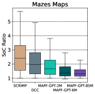
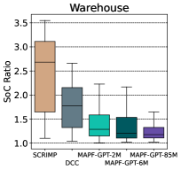
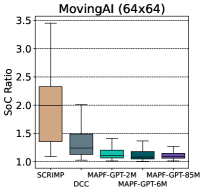
Figure 4: Performance of MAPF approaches on Random, Mazes, Warehouse and MovingAI maps, based on SoC metric relative to LaCAM performance (lower is better).

Model Training

As the model backbone, we used a modern decoder-only transformer (Brown et al. 2020). We used a softmax layer to parameterize the discrete probability distribution. To sample an action, we then used multinomial sampling. The length of the input sequence (context size) of the model is $256$. The output size of the model is $5$ since each agent has $5$ available discrete actions. We used learnable position embeddings. Our largest model has $85$M parameters. Besides it, we also trained models with $6$M and $2$M parameters. We don’t use causal masking, which is common practice in NLP (Radford et al. 2019), since the model predicts only a single action ahead in a non-autoregressive manner. To speed up training, we used the flash attention technique (Dao 2024).

Training protocol

The model was trained to replicate the behavior of the expert policy using cross-entropy loss (i.e., log-loss) via mini-batch stochastic gradient descent, optimized with AdamW (Loshchilov and Hutter 2019). The target label for this loss is the ground-truth action index provided by the expert policy, LaCAM. LaCAM is a centralized solver that builds a path for all agents during the whole episode, leveraging information about the full environment state. In contrast, the trainable model relies solely on the local observation $o$ of each agent $u$.

$$-\log\textbf{p}_{\theta}\left(a_{u}^{LaCAM}(s)\mid o_{u}\right).$$ (1)

After training, this policy allows actions to be sampled from it. While an alternative could be to pick the action with the highest probability, we use sampling, recognizing the decentralized nature of the policy. Sampling selects actions according to the probability distribution given by the policy:

$$\hat{a}^{u}(o_{u})\sim\textbf{p}_{\theta}(o_{u})$$ (2)

where $\textbf{p}_{\theta}(o_{u})$ represents the probability distribution over actions computed by the model for the observation $o_{u}$.

We used $2000$ warm-up iterations and cosine annealing (Loshchilov and Hutter 2017), with a gradient clipping value of $1.0$ and a weight decay parameter of $0.1$. The entire 1B dataset was utilized to train the 85M model, which underwent 1M iterations with a batch size of $512$, resulting in $15.625$ epochs based on the gradient accumulation steps, set at $16$. For training the 6M and 2M models, we used portions of the 1B dataset – 150M and 40M, respectively. Additional details about the parameters influencing the training process are provided in the Appendix.

Experimental Evaluation

Main results

In the first series of experiments, we compare 3 variants of MAPF-GPT varying in the number of parameters in their neural networks (2M, 6M, 85M) with the state-of-the-art learnable MAPF solvers: DCC (Ma, Luo, and Pan 2021) and SCRIMP (Wang et al. 2023). We use the pre-trained weights for DCC and SCRIMP. These weights were obtained by the authors while training on the random maps. Additionally, we present the results of LaCAM (Okumura 2024), which served as the expert centralized solver for data collection. For evaluation we used Random, Mazes, Warehouse, MovingAI maps (the latter two are out-of-distribution for all learnable solvers). The details on the maps and problem instances are given in the Appendix.

The results are presented in Figure 3, where the success rate of all solvers is shown. Clearly, MAPF-GPTs significantly outperform DCC and SCRIMP across all scenarios, with the largest model, MAPF-GPT-85M, being the absolute leader. MAPF-GPT-6M shows slightly better results on the Random and Mazes maps, and comparable results on the Warehouse and MovingAI maps to the smallest MAPF-GPT-2M model.

Figure 4 shows the Sum-of-Costs (SoC) achieved by the solvers relative to SoC of LaCAM (the lower - the better). As can be seen, MAPF-GPTs again outperform the other approaches and their performance correlates with the number of model parameters. Interestingly, there are some rare cases on Random maps where DCC and MAPF-GPT-85M outperformed LaCAM in terms of SoC. The same situation is observed for MAPF-GPT-6M on Mazes maps.

Runtime

In this experiment, we compare the runtime efficiency of each approach. The results are presented in Figure 5; each data point indicates the average time spent deciding the next action for all agents. All MAPF-GPT models scale linearly with the increasing number of agents. The largest model, MAPF-GPT-85M, shows a slightly higher runtime than DCC and SCRIMP with up to 96 agents. However, beyond 128 agents, the runtime is better, as it depends linearly on the number of agents. Notably, the MAPF-GPT-2M and MAPF-GPT-6M models are more than 13 times faster than SCRIMP and 8 times faster than DCC for 192 agents setup.

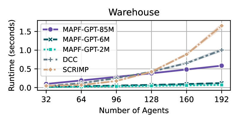
Figure 5: Runtime comparison of MAPF-GPT, DCC, and SCRIMP models on the warehouse environment. The plot shows the average time required to decide the next action for all agents as the number of agents increases.

Ablation study

In this experiment, we study how each part of the information influences the performance of the MAPF-GPT agent. To address this, we trained a 6M parameter model with certain pieces of information masked that were provided to the original model. We examine four different cases: if there is no goal information for all agents (noGoal), if there is no greedy action provided (noGA), if there is no action history (noAH), and if the agent is trained without cost-to-go information (still retaining information about obstacles). The results are presented in Table 1.

Table 1: Success rates of different versions of MAPF-GPT-6M on all sets of maps from POGEMA benchmark.

Dataset	6M	noGoal	noGA	noAH	noC2G
Random	97.6%	95.7%	97.0%	95.6%	25.8%
Mazes	74.6%	71.6%	37.6%	85.8%	15.1%
Warehouse	94.1%	92.8%	87.7%	94.8%	11.5%
MovingAI	82.0%	88.4%	79.1%	82.2%	10.2%
Puzzles	94.0%	92.7%	92.7%	91.5%	52.5%

As can be seen, the 6M model without masking shows better results on the Random and Puzzles maps. The model trained without goal information shows better results on the MovingAI maps, with $88.4\%$ compared to $82.0\%$ for the original model. This improvement is likely due to the large map sizes, where most conflicts arise during the agents’ movement toward their goals, making the exact goal coordinates less critical. Additionally, the functionality was compensated by the greedy action, which indicates the direction to the goal.

Surprisingly, the model trained without action history shows better performance on the Mazes and Warehouse instances. This suggests that action history is not crucial for behavioral cloning, as LaCAM does not rely on it. Despite these results, we argue for retaining movement history information in the agent’s observation, which could be essential for fine-tuning the model in the environment using RL technique.

Masking greedy action and cost-to-go information degrades the performance of the model on all the testing tasks, highlighting their crucial role in effective pathfinding and conflict resolution.

LifeLong MAPF

In addition to evaluating MAPF-GPT on the MAPF instances it was trained on, we also assessed its performance in a Life-Long MAPF (LMAPF) setup. Unlike regular MAPF problems, in LMAPF, each agent receives a new goal location every time it reaches its current one. In this setup, the primary objective is throughput, which is defined as the average number of goals reached by all agents per time step.

We evaluated MAPF-GPT in both zero-shot and fine-tuned configurations. To fine-tune the model, we generated an additional dataset using Mazes maps. For expert data, we employed the RHCR approach (Li et al. 2021), as LaCAM is not well-suited for LMAPF. The dataset contains 90 million (observation, action) pairs. We used MAPF-GPT-6M for this experiment.

The results are presented in Table 2. Even the zero-shot model is able to compete with other existing learning-based approaches, such as Follower (Skrynnik et al. 2024b) and MATS-LP (Skrynnik et al. 2024c). Moreover, in all cases, fine-tuning improved the results of the MAPF-GPT-6M model.

Table 2: Average throughput (higher is better) of MAPF-GPT-6M both in zero-shot mode and after fine-tuning compared to RHCR, Follower and MATS-LP.

	Random	Mazes	Warehouse	MovingAI
MAPF-GPT-6M	1.497	0.908	1.113	2.840
MAPF-GPT-6M-t	1.507	1.087	1.270	2.994
RHCR	2.164	1.554	2.352	3.480
Follower	1.637	1.140	2.731	3.271
MATS-LP	1.674	1.125	1.701	3.320

These results demonstrate the ability of MAPF-GPT to perform zero-shot learning, i.e., the ability to solve types of problems that it was not initially designed for (e.g., solving LMAPF instead of MAPF), and that fine-tuning MAPF-GPT is indeed possible, i.e., additional training on new types of tasks increases its performance in solving these tasks.

Conclusion

In this work, we studied the MAPF problem as a sequential decision-making task. We proposed an approach to derive an individual policy based on state-of-the-art machine learning techniques, specifically (supervised) imitation learning from expert data —- MAPF-GPT. To train MAPF-GPT, we created a comprehensive dataset of expert MAPF solutions, transformed these solutions into (observation, action) pairs, tokenized them, and trained several transformer models (with varying numbers of parameters) on this data. Empirically, we demonstrate that even with a quite moderate number of parameters, such as 2M, MAPF-GPT significantly outperforms modern learnable MAPF competitors across a wide range of setups. Our results provide a clear positive answer to the question, ”Is it possible to create a strong learnable MAPF solver purely through imitation learning?”. The limitations of our approach are discussed in the Appendix.

Appendix A Appendix

Appendix B Implementation Details

The open-sourced repository contains all the necessary resources to replicate the results of MAPF-GPT. This includes scripts for dataset generation, training, evaluation. The codebase also provides example scripts to help users quickly understand and run MAPF-GPT, along with the detailed instructions for setting up the environment using Docker. Additionally, configuration files for benchmarks and datasets are included to facilitate effortless replication of the experiments.

The GPT model’s code is primarily based on the NanoGPT codebase. NanoGPT was chosen for its simple yet modular design, making it easier to modify and adapt the code, including potential adjustments for fine-tuning in environment (e.g., with reinforcement learning).

Appendix C Hyperparameters and Training Details

This section details the hyperparameters used while training all three our models: MAPF-GPT-2M, MAPF-GPT-6M, and MAPF-GPT-85M. Common parameters for the models are listed in Table 3.

Table 3: Common hyperparameters for MAPF-GPT models.

Parameter	Value
Minimum learning rate	6e-5
Maximum learning rate	6e-4
Learning rate decay	cosine
Warm-up iterations	2000
AdamW optimizer beta1	0.9
AdamW optimizer beta2	0.95
Gradient clipping	1.0
Weight decay	1e-1
Data type for computations	float16
Use PyTorch 2.0 compilation	True
Gradient accumulation steps	16
Block size	256

Table 4 provides model-specific hyperparameters for MAPF-GPT-2M, MAPF-GPT-6M, and MAPF-GPT-85M. We didn’t change the hyperparameters between the models except for those that influence their size and the duration of the learning process. Training the 85M model for 1M iterations took 243 hours using 4x H100 80GB NVIDIA GPUs. Training the 6M model for 30K iterations took 50 hours using 2x A100 80GB NVIDIA GPUs. The 2M model was trained on a single H100 80GB NVIDIA GPU within 12 hours. It is also worth noting that while training the 6M and 2M models we could not fully utilize the computational power of the corresponding GPUs, as the bottleneck was actually in data processing and transferring it to the GPU.

Table 4: Model-specific hyperparameters.

Parameter	2M	6M	85M
Number of epochs	46.875	12.5	15.625
Total training iterations	15,000	30,000	1,000,000
Batch size	4096	2048	512
Number of layers	5	8	12
Number of attention heads	5	8	12
Embedding size	160	256	768

The loss curves for MAPF-GPT-85M are presented in Figure 6, showing the averaged loss for both training and validation. The validation dataset contains an equal 1:1 ratio of (observation, action) pairs between maze-like and random maps, in contrast to the 9:1 ratio in the training dataset.

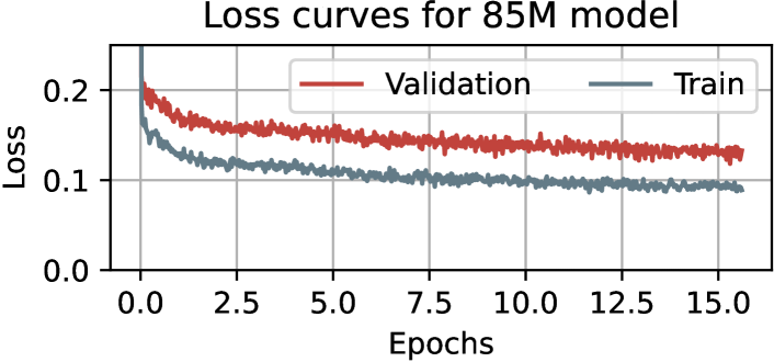
Figure 6: Training and validation loss curves for MAPF-GPT-85M.

During training, we also performed evaluations in the environment using intermediate checkpoints. The aggregated results of these evaluations are presented in Figure 7. Intermediate evaluations were conducted on 6 random maps with 48 and 64 agents, as well as 6 maze maps with 32 and 48 agents. These maps were taken from the set used to generate the validation dataset.

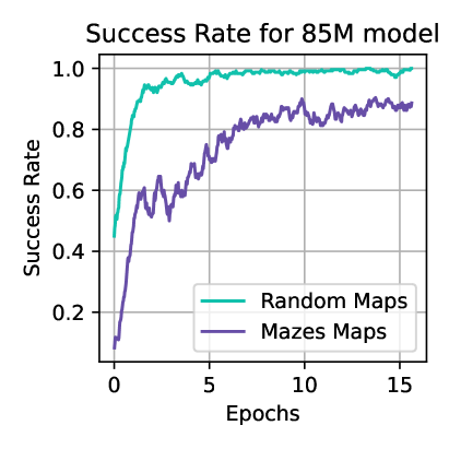
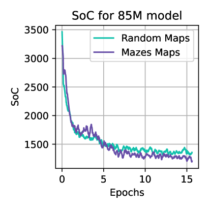
Figure 7: Aggregated evaluation results for Success rate and Sum of Costs during training.

Appendix D Dataset: Technical Details

As mentioned in the main part of the text, to generate the 1B training dataset, we first generated 10,000 maps using a maze generator and 2,500 maps using a random map generator. Next, we generated instances with 16, 24, or 32 agents, with 100 seeds (start-goal locations) per map, resulting in 3.75M different instances.

In the next step, we ran the centralized MAPF solver, i.e. LaCAM, to obtain the expert data. We used the latest version of LaCAM and its C++ implementation provided by the authors. LaCAM was given 10 seconds to solve each instance in a single-thread mode. We ran LaCAM in parallel on two workstations with AMD Ryzen Threadripper 3970X 32-Core Processors, which took nearly 100 hours to obtain the data. Around 3% of the instances were not successfully solved (primarily those with 32 agents) due to the presence of unsolvable tasks and a time limit.

The resulting log files, which contain the actions taken by the agents at each time step, were evenly distributed into $50$ chunks. The logs from each chunk were processed to generate local observations for every agent. At this stage, we removed redundant waiting actions and duplicate observations as detailed in the main body of the paper.

In the final step, the obtained data was shuffled and saved into $10$ .arrow files per chunk. Each .arrow file contains $2^{21}$(slightly more than 2 million) (observation, action) pairs, with 10% of the data coming from the random maps and 90% – from mazes.

The resultant 1B dataset contains 500 such files, requiring 258GB of disk space. While training the MAPF-GPT-6M and MAPF-GPT-2M models, we randomly selected 75 and 20 files from this dataset, resulting in 150M and 40M datasets, respectively. The full dataset was used for training MAPF-GPT-85M model. The sizes of the datasets were selected according to Chinchilla paper (Hoffmann et al. 2022), which empirically found a scaling law of 20 tokens per model parameter, demonstrating the efficiency of a 70-billion-parameter model trained on 1.4 trillion tokens compared to larger models trained on fewer tokens.

Appendix E Benchmark

For empirical evaluation we have utilized the evaluation tools provided by the POGEMA benchmark (Skrynnik et al. 2024a). Specifically, we used the following set of maps: Random, Mazes, Warehouse (Li et al. 2021), MovingAI (Stern et al. 2019) and Puzzles. Table 5 contains information about the number of agents, maps, and instances per map (seeds) used in each set.

Table 5: Details about different sets of maps from POGEMA benchmark.

Set	Agents	Maps	Map Size	Seeds	Steps
Random	8, 16, 24, 32, 48, 64	128	17$\times$17 - 21$\times$21	1	128
Mazes	8, 16, 24, 32, 48, 64	128	17$\times$17 - 21$\times$21	1	128
Warehouse	32, 64, 96, 128, 160, 192	1	33$\times$46	128	128
MovingAI	64, 128, 192, 256	128	64$\times$64	1	256
Puzzles	2, 3, 4	16	5$\times$5	10	128

(a) Random

(b) Mazes

(c) Warehouse

Figure 8: The examples of maps from the POGEMA benchmark. Plots show the maximum number of agents tested on each map: 64 agents for Random and Mazes sets, and 192 agents for Warehouse scenario.

Figure 8 showcases examples of maps from the POGEMA benchmark. The Mazes and Random map sets are generated using the built-in generators within POGEMA. The Puzzles maps are handcrafted. The Warehouse is a single map with limitations on possible start and goal positions, which has been used in previous LMAPF-related studies (Li et al. 2021; Skrynnik et al. 2024b). Start locations on this map can only be generated on the left or right sides of the map, where there are no obstacles, while goal locations can only be placed beyond or below the obstacles in the center of the map. These constraints prevent the generation of instances with more than 192 agents on this map.

The final evaluated set of maps is MovingAI, referred to as MovingAI-tiles in the POGEMA benchmark. While the original MovingAI dataset includes various types of maps, including random and maze maps, the MovingAI-tiles set in POGEMA contains only city maps. Additionally, due to the large size ($256\times 256$) of city maps, they were divided into 16 tiles, resulting in maps of $64\times 64$ size. An example of such scenario is presented in Figure 9.

Figure 9: Example of a city map from the MovingAI-tiles set in the POGEMA benchmark. The original city maps, with dimensions of $256\times 256$, were divided into 16 tiles, resulting in smaller $64\times 64$ maps.

The evaluation of all the approaches, including the MAPF-GPT models and the baselines, was performed on the same workstation equipped with AMD Ryzen Threadripper 3970X 32-Core Processors, 256GB of RAM, and 2x RTX 3080 Ti 12GB NVIDIA GPUs.

It’s important to note that during the runtime experiments, only one GPU was utilized, and the tasks were run in sequential mode, i.e., no multiple tasks were executed in parallel during this experiment. For this evaluation, we ran all approaches on the Warehouse map with 32 to 192 agents, using five different seeds, and averaged the obtained results.

Appendix F Limitations

The main limitation of MAPF-GPT is a generic one, shared with the other learnable methods, i.e. it lacks theoretical guarantees. The next limitation is that training large models, e.g., MAPF-GPT-85M, is quite demanding (requires expensive hardware and prolonged time). Still, our smaller models containing 6M and 2M parameters are much less demanding while providing competitive results. It should also be noted that all MAPF-GPT models are sensitive to the quality of trajectories in the expert data set. As has been shown in previous research on behavior cloning with transformers, e.g. (Chen et al. 2021), adding low-quality trajectories to expert data may lead to significant degradation in model’s performance. It is also unclear how effectively MAPF-GPT can replicate the behavior of the other existing centralized approaches (such as CBS (Sharon et al. 2015) that is an optimal MAPF solver). This dependence on the type of behavioral expert policy requires further research.

Appendix G Evaluation on Puzzles

The Puzzles set is part of the POGEMA benchmark, briefly mentioned in the ablation study section of our paper. However, it provides valuable insights into the cooperation abilities of agents. The Puzzles maps were specifically designed with narrow corridors, cul-de-sacs, and lacunas. The examples of such scenarios are depicted in Figure 10. These challenging instances require agents to cooperate strategically, such as one agent entering a corridor and using a lacuna to let another agent pass.

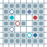
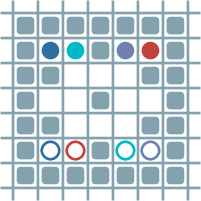
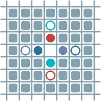
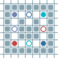
Figure 10: Examples of Puzzles map instances. This set of scenarios is particularly challenging and requires high cooperation between agents.

The results are presented in Table 6. During testing, there were 2 to 4 agents on each map. Among the learnable approaches, the MAPF-GPT family performed the best, with performance depending on the number of model parameters. The 85M model performs the best for both metrics (success rate and SoC). Interestingly, its success rate is very close to that of LaCAM on some instances. However, LaCAM significantly outperforms all other approaches in terms of SoC. DCC and SCRIMP show much lower results on both metrics. Even for the simplest tasks with two agents, the SoC of DCC and SCRIMP is 2.5 times higher than that of MAPF-GPT-85M and almost 3 times higher than that of LaCAM.

Table 6: Comparison of algorithms on Puzzles set, with varying number of agents. $\pm$ shows confidence intervals $95\%$.

Algorithm	Success Rate $\uparrow$	SoC $\downarrow$
Number of agents: 2
MAPF-GPT-85M	$1.00$ p m 0.00	$11.97$ p m 1.32
MAPF-GPT-6M	$1.00$ p m 0.00	$14.14$ p m 2.65
MAPF-GPT-2M	$0.99$ p m 0.02	$18.28$ p m 5.42
DCC	$0.91$ p m 0.04	$31.49$ p m 9.38
SCRIMP	$0.94$ p m 0.03	$33.52$ p m 9.70
LaCAM	$1.00$ p m 0.00	$10.96$ p m 1.15
Number of agents: 3
MAPF-GPT-85M	$0.94$ p m 0.03	$42.08$ p m 12.22
MAPF-GPT-6M	$0.94$ p m 0.03	$49.48$ p m 13.45
MAPF-GPT-2M	$0.93$ p m 0.04	$60.22$ p m 15.45
DCC	$0.75$ p m 0.07	$86.73$ p m 16.71
SCRIMP	$0.82$ p m 0.06	$93.31$ p m 19.91
LaCAM	$0.96$ p m 0.03	$34.89$ p m 11.37
Number of agents: 4
MAPF-GPT-85M	$0.92$ p m 0.04	$99.93$ p m 22.59
MAPF-GPT-6M	$0.88$ p m 0.05	$124.15$ p m 25.43
MAPF-GPT-2M	$0.81$ p m 0.06	$136.50$ p m 27.19
DCC	$0.51$ p m 0.08	$170.77$ p m 20.53
SCRIMP	$0.70$ p m 0.07	$186.10$ p m 27.51
LaCAM	$0.94$ p m 0.03	$63.02$ p m 17.97

References

- Alkazzi and Okumura (2024) Alkazzi, J.-M.; and Okumura, K. 2024. A Comprehensive Review on Leveraging Machine Learning for Multi-Agent Path Finding. IEEE Access.
- Baker et al. (2022) Baker, B.; Akkaya, I.; Zhokov, P.; Huizinga, J.; Tang, J.; Ecoffet, A.; Houghton, B.; Sampedro, R.; and Clune, J. 2022. Video pretraining (vpt): Learning to act by watching unlabeled online videos. Advances in Neural Information Processing Systems, 35: 24639–24654.
- Bhattacharyya et al. (2018) Bhattacharyya, R. P.; Phillips, D. J.; Wulfe, B.; Morton, J.; Kuefler, A.; and Kochenderfer, M. J. 2018. Multi-agent imitation learning for driving simulation. In 2018 IEEE/RSJ International Conference on Intelligent Robots and Systems (IROS), 1534–1539. IEEE.
- Brown et al. (2020) Brown, T.; Mann, B.; Ryder, N.; Subbiah, M.; Kaplan, J. D.; Dhariwal, P.; Neelakantan, A.; Shyam, P.; Sastry, G.; Askell, A.; Agarwal, S.; Herbert-Voss, A.; Krueger, G.; Henighan, T.; Child, R.; Ramesh, A.; Ziegler, D.; Wu, J.; Winter, C.; Hesse, C.; Chen, M.; Sigler, E.; Litwin, M.; Gray, S.; Chess, B.; Clark, J.; Berner, C.; McCandlish, S.; Radford, A.; Sutskever, I.; and Amodei, D. 2020. Language Models are Few-Shot Learners. In Larochelle, H.; Ranzato, M.; Hadsell, R.; Balcan, M.; and Lin, H., eds., Advances in Neural Information Processing Systems, volume 33, 1877–1901. Curran Associates, Inc.
- Chen et al. (2021) Chen, L.; Lu, K.; Rajeswaran, A.; Lee, K.; Grover, A.; Laskin, M.; Abbeel, P.; Srinivas, A.; and Mordatch, I. 2021. Decision transformer: Reinforcement learning via sequence modeling. Advances in neural information processing systems, 34: 15084–15097.
- Chi et al. (2023) Chi, C.; Feng, S.; Du, Y.; Xu, Z.; Cousineau, E.; Burchfiel, B.; and Song, S. 2023. Diffusion Policy: Visuomotor Policy Learning via Action Diffusion. In Proceedings of Robotics: Science and Systems (RSS).
- Damani et al. (2021) Damani, M.; Luo, Z.; Wenzel, E.; and Sartoretti, G. 2021. PRIMAL : Pathfinding via reinforcement and imitation multi-agent learning-lifelong. IEEE Robotics and Automation Letters, 6(2): 2666–2673.
- Dao (2024) Dao, T. 2024. FlashAttention-2: Faster Attention with Better Parallelism and Work Partitioning. In The Twelfth International Conference on Learning Representations.
- Dubey et al. (2024) Dubey, A.; Jauhri, A.; Pandey, A.; Kadian, A.; Al-Dahle, A.; Letman, A.; Mathur, A.; Schelten, A.; Yang, A.; Fan, A.; et al. 2024. The llama 3 herd of models. arXiv preprint arXiv:2407.21783.
- Fujimoto and Gu (2021) Fujimoto, S.; and Gu, S. S. 2021. A minimalist approach to offline reinforcement learning. Advances in neural information processing systems, 34: 20132–20145.
- Hoffmann et al. (2022) Hoffmann, J.; Borgeaud, S.; Mensch, A.; Buchatskaya, E.; Cai, T.; Rutherford, E.; de Las Casas, D.; Hendricks, L. A.; Welbl, J.; Clark, A.; et al. 2022. Training compute-optimal large language models. In Proceedings of the 36th International Conference on Neural Information Processing Systems, 30016–30030.
- Huang et al. (2023) Huang, C.; Zhao, J.; Zhou, H.; Zhang, H.; Zhang, X.; and Ye, C. 2023. Multi-agent Decision-making at Unsignalized Intersections with Reinforcement Learning from Demonstrations. In 2023 IEEE Intelligent Vehicles Symposium (IV), 1–6. IEEE.
- Kostrikov, Nair, and Levine (2022) Kostrikov, I.; Nair, A.; and Levine, S. 2022. Offline Reinforcement Learning with Implicit Q-Learning. In International Conference on Learning Representations.
- Kumar et al. (2020) Kumar, A.; Zhou, A.; Tucker, G.; and Levine, S. 2020. Conservative q-learning for offline reinforcement learning. Advances in Neural Information Processing Systems, 33: 1179–1191.
- Le et al. (2017) Le, H. M.; Yue, Y.; Carr, P.; and Lucey, P. 2017. Coordinated multi-agent imitation learning. In International Conference on Machine Learning, 1995–2003. PMLR.
- Levine et al. (2020) Levine, S.; Kumar, A.; Tucker, G.; and Fu, J. 2020. Offline reinforcement learning: Tutorial, review, and perspectives on open problems. arXiv preprint arXiv:2005.01643.
- Li et al. (2022) Li, J.; Chen, Z.; Harabor, D.; Stuckey, P. J.; and Koenig, S. 2022. MAPF-LNS2: Fast repairing for multi-agent path finding via large neighborhood search. In Proceedings of the AAAI Conference on Artificial Intelligence, volume 36, 10256–10265.
- Li et al. (2021) Li, J.; Tinka, A.; Kiesel, S.; Durham, J. W.; Kumar, T. S.; and Koenig, S. 2021. Lifelong multi-agent path finding in large-scale warehouses. In Proceedings of the 35th AAAI Conference on Artificial Intelligence (AAAI 2021), 11272–11281.
- Li et al. (2024) Li, W.; Huang, S.; Qiu, Z.; and Song, A. 2024. GAILPG: Multi-Agent Policy Gradient with Generative Adversarial Imitation Learning. IEEE Transactions on Games.
- Liu et al. (2024) Liu, H.; Li, C.; Wu, Q.; and Lee, Y. J. 2024. Visual instruction tuning. Advances in neural information processing systems, 36.
- Liu and Zhu (2024) Liu, S.; and Zhu, M. 2024. Learning multi-agent behaviors from distributed and streaming demonstrations. Advances in Neural Information Processing Systems, 36.
- Lopez et al. (2018) Lopez, P. A.; Behrisch, M.; Bieker-Walz, L.; Erdmann, J.; Flötteröd, Y.-P.; Hilbrich, R.; Lücken, L.; Rummel, J.; Wagner, P.; and Wießner, E. 2018. Microscopic traffic simulation using sumo. In 2018 21st international conference on intelligent transportation systems (ITSC), 2575–2582. IEEE.
- Loshchilov and Hutter (2017) Loshchilov, I.; and Hutter, F. 2017. SGDR: Stochastic Gradient Descent with Warm Restarts. In International Conference on Learning Representations.
- Loshchilov and Hutter (2019) Loshchilov, I.; and Hutter, F. 2019. Decoupled Weight Decay Regularization. In International Conference on Learning Representations.
- Ma et al. (2019) Ma, H.; Harabor, D.; Stuckey, P. J.; Li, J.; and Koenig, S. 2019. Searching with consistent prioritization for multi-agent path finding. In Proceedings of the AAAI conference on artificial intelligence, volume 33, 7643–7650.
- Ma, Luo, and Pan (2021) Ma, Z.; Luo, Y.; and Pan, J. 2021. Learning selective communication for multi-agent path finding. IEEE Robotics and Automation Letters, 7(2): 1455–1462.
- Meng et al. (2021) Meng, L.; Wen, M.; Yang, Y.; Le, C.; Li, X.; Zhang, W.; Wen, Y.; Zhang, H.; Wang, J.; and Xu, B. 2021. Offline pre-trained multi-agent decision transformer: One big sequence model tackles all smac tasks. arXiv preprint arXiv:2112.02845.
- Mironov et al. (2023) Mironov, K.; Yudin, D.; Alhaddad, M.; Makarov, D.; Pushkarev, D.; Linok, S.; Belkin, I.; Krishtopik, A.; Golovin, V.; Yakovlev, K.; et al. 2023. STRL-Robotics: intelligent control for robotic platform in human-oriented environment. Artificial Intelligence and Decision Making, 45–63.
- Okumura (2023) Okumura, K. 2023. Lacam: Search-based algorithm for quick multi-agent pathfinding. In Proceedings of the AAAI Conference on Artificial Intelligence, volume 37, 11655–11662.
- Okumura (2024) Okumura, K. 2024. Engineering LaCAM*: Towards Real-time, Large-scale, and Near-optimal Multi-agent Pathfinding. In Proceedings of the 23rd International Conference on Autonomous Agents and Multiagent Systems, 1501–1509.
- Radford et al. (2019) Radford, A.; Wu, J.; Child, R.; Luan, D.; Amodei, D.; and Sutskever, I. 2019. Language Models are Unsupervised Multitask Learners. OpenAI blog.
- Ruoss et al. (2024) Ruoss, A.; Delétang, G.; Medapati, S.; Grau-Moya, J.; Wenliang, L. K.; Catt, E.; Reid, J.; and Genewein, T. 2024. Grandmaster-level chess without search. arXiv preprint arXiv:2402.04494.
- Samvelyan et al. (2019) Samvelyan, M.; Rashid, T.; Schroeder de Witt, C.; Farquhar, G.; Nardelli, N.; Rudner, T. G.; Hung, C.-M.; Torr, P. H.; Foerster, J.; and Whiteson, S. 2019. The StarCraft Multi-Agent Challenge. In Proceedings of the 18th International Conference on Autonomous Agents and MultiAgent Systems, 2186–2188.
- Sharon et al. (2015) Sharon, G.; Stern, R.; Felner, A.; and Sturtevant, N. R. 2015. Conflict-based search for optimal multi-agent pathfinding. Artificial intelligence, 219: 40–66.
- Sharon et al. (2013) Sharon, G.; Stern, R.; Goldenberg, M.; and Felner, A. 2013. The increasing cost tree search for optimal multi-agent pathfinding. Artificial intelligence, 195: 470–495.
- Shih, Ermon, and Sadigh (2022) Shih, A.; Ermon, S.; and Sadigh, D. 2022. Conditional imitation learning for multi-agent games. In 2022 17th ACM/IEEE International Conference on Human-Robot Interaction (HRI), 166–175. IEEE.
- Silver et al. (2016) Silver, D.; Huang, A.; Maddison, C. J.; Guez, A.; Sifre, L.; Van Den Driessche, G.; Schrittwieser, J.; Antonoglou, I.; Panneershelvam, V.; Lanctot, M.; et al. 2016. Mastering the game of Go with deep neural networks and tree search. nature, 529(7587): 484–489.
- Silver et al. (2017) Silver, D.; Schrittwieser, J.; Simonyan, K.; Antonoglou, I.; Huang, A.; Guez, A.; Hubert, T.; Baker, L.; Lai, M.; Bolton, A.; et al. 2017. Mastering the game of go without human knowledge. nature, 550(7676): 354–359.
- Skrynnik et al. (2024a) Skrynnik, A.; Andreychuk, A.; Borzilov, A.; Chernyavskiy, A.; Yakovlev, K.; and Panov, A. 2024a. POGEMA: A Benchmark Platform for Cooperative Multi-Agent Navigation. arXiv preprint arXiv:2407.14931.
- Skrynnik et al. (2024b) Skrynnik, A.; Andreychuk, A.; Nesterova, M.; Yakovlev, K.; and Panov, A. 2024b. Learn to Follow: Decentralized Lifelong Multi-agent Pathfinding via Planning and Learning. In Proceedings of the 38th AAAI Conference on Artificial Intelligence (AAAI 2024).
- Skrynnik et al. (2024c) Skrynnik, A.; Andreychuk, A.; Yakovlev, K.; and Panov, A. 2024c. Decentralized Monte Carlo Tree Search for Partially Observable Multi-Agent Pathfinding. In Proceedings of the AAAI Conference on Artificial Intelligence, volume 38, 17531–17540.
- Skrynnik et al. (2021) Skrynnik, A.; Yakovleva, A.; Davydov, V.; Yakovlev, K.; and Panov, A. I. 2021. Hybrid policy learning for multi-agent pathfinding. IEEE Access, 9: 126034–126047.
- Song et al. (2018) Song, J.; Ren, H.; Sadigh, D.; and Ermon, S. 2018. Multi-agent generative adversarial imitation learning. Advances in neural information processing systems, 31.
- Stern et al. (2019) Stern, R.; Sturtevant, N. R.; Felner, A.; Koenig, S.; Ma, H.; Walker, T. T.; Li, J.; Atzmon, D.; Cohen, L.; Kumar, T. S.; et al. 2019. Multi-agent pathfinding: Definitions, variants, and benchmarks. In Proceedings of the 12th Annual Symposium on Combinatorial Search (SoCS 2019), 151–158.
- Surynek (2010) Surynek, P. 2010. An optimization variant of multi-robot path planning is intractable. In Proceedings of the 24th AAAI Conference on Artificial Intelligence (AAAI 2010), 1261–1263.
- Surynek et al. (2016) Surynek, P.; Felner, A.; Stern, R.; and Boyarski, E. 2016. Efficient SAT approach to multi-agent path finding under the sum of costs objective. In Proceedings of the 22nd European Conference on Artificial Intelligence (ECAI 2016), 810–818. IOS Press.
- Svancara and Barták (2022) Svancara, J.; and Barták, R. 2022. Tackling Train Routing via Multi-agent Pathfinding and Constraint-based Scheduling. In Proceedings of The 14th International Conference on Agents and Artificial Intelligence (ICAART 2022), 306–313.
- Tang et al. (2024) Tang, J.; Swamy, G.; Fang, F.; and Wu, Z. S. 2024. Multi-Agent Imitation Learning: Value is Easy, Regret is Hard. arXiv preprint arXiv:2406.04219.
- Vaswani et al. (2023) Vaswani, A.; Shazeer, N.; Parmar, N.; Uszkoreit, J.; Jones, L.; Gomez, A. N.; Kaiser, L.; and Polosukhin, I. 2023. Attention Is All You Need. arXiv:1706.03762.
- Vinyals et al. (2019) Vinyals, O.; Babuschkin, I.; Czarnecki, W. M.; Mathieu, M.; Dudzik, A.; Chung, J.; Choi, D. H.; Powell, R.; Ewalds, T.; Georgiev, P.; et al. 2019. Grandmaster level in StarCraft II using multi-agent reinforcement learning. nature, 575(7782): 350–354.
- Wagner and Choset (2011) Wagner, G.; and Choset, H. 2011. M*: A complete multirobot path planning algorithm with performance bounds. In Proceedings of The 2011 IEEE/RSJ International Conference on Intelligent Robots and Systems (IROS 2011), 3260–3267.
- Wang et al. (2021) Wang, H.; Yu, L.; Cao, Z.; and Ermon, S. 2021. Multi-agent imitation learning with copulas. In Machine Learning and Knowledge Discovery in Databases. Research Track: European Conference, ECML PKDD 2021, Bilbao, Spain, September 13–17, 2021, Proceedings, Part I 21, 139–156. Springer.
- Wang et al. (2023) Wang, Y.; Xiang, B.; Huang, S.; and Sartoretti, G. 2023. SCRIMP: Scalable communication for reinforcement-and imitation-learning-based multi-agent pathfinding. In 2023 IEEE/RSJ International Conference on Intelligent Robots and Systems (IROS), 9301–9308. IEEE.
- Yang et al. (2020) Yang, F.; Vereshchaka, A.; Chen, C.; and Dong, W. 2020. Bayesian multi-type mean field multi-agent imitation learning. Advances in Neural Information Processing Systems, 33: 2469–2478.
- Yu and LaValle (2013) Yu, J.; and LaValle, S. M. 2013. Multi-agent path planning and network flow. In Algorithmic Foundations of Robotics X: Proceedings of the Tenth Workshop on the Algorithmic Foundations of Robotics, 157–173. Springer.
- Zhu et al. (2024) Zhu, D.; Chen, J.; Shen, X.; Li, X.; and Elhoseiny, M. 2024. MiniGPT-4: Enhancing Vision-Language Understanding with Advanced Large Language Models. In The Twelfth International Conference on Learning Representations.