Latent-EnSF: A Latent Ensemble Score Filter for High-Dimensional Data Assimilation with Sparse Observation Data

Abstract

Accurate modeling and prediction of complex physical systems often rely on data assimilation techniques to correct errors inherent in model simulations. Traditional methods like the Ensemble Kalman Filter (EnKF) and its variants as well as the recently developed Ensemble Score Filters (EnSF) face significant challenges when dealing with high-dimensional and nonlinear Bayesian filtering problems with sparse observations, which are ubiquitous in real-world applications. In this paper, we propose a novel data assimilation method, Latent-EnSF, which leverages EnSF with efficient and consistent latent representations of the full states and sparse observations to address the joint challenges of high dimensionlity in states and high sparsity in observations for nonlinear Bayesian filtering. We introduce a coupled Variational Autoencoder (VAE) with two encoders to encode the full states and sparse observations in a consistent way guaranteed by a latent distribution matching and regularization as well as a consistent state reconstruction. With comparison to several methods, we demonstrate the higher accuracy, faster convergence, and higher efficiency of Latent-EnSF for two challenging applications with complex models in shallow water wave propagation and medium-range weather forecasting, for highly sparse observations in both space and time.

1 Introduction

Many complex physical systems are traditionally modeled by partial differential equations (PDEs). First-principle PDE-based modeling and simulation have been demonstrated to be powerful in making predictions of complex systems in various scientific and engineering fields. However, in practical applications, significant discrepancy of the simulation-based prediction and the reality may arise from different sources, e.g., model inadequacy, uncertainties in model parameters, boundary and/or initial conditions, exteral forcing/loading terms, numerical approximation errors, etc. Meanwhile, data-driven machine learning (ML) models have been significantly developed and employed to make system predictions in the last few years, which have been shown to be extremely efficient in the case of large dynamical systems such as weather forecasting, a problem that requires the supercomputer of hours to run for the European Centre for Medium-Range Weather Forecasts (ECMWF), but one that can be solved by neural network surrogates such as FourCastNet (Pathak et al., 2022) in a matter of seconds. These properties also make them particularly suitable for ensemble forecasting and uncertainty quantification. However, these models are also often subject to the key limitation of divergence from reality in the long run, resulting in significant accumulated errors for long-term predictions because of various uncertainties and the autoregressive structure of the ML models.

To mitigate the discrepancy and accumulated errors and make more accurate predictions, data assimilation plays an essential role in incorporating additional observation data of the reality into the current PDE/ML-based prediction models. By adapting the PDE/ML state to match the observation data, the accuracy of future state predictions can be markedly improved. Data assimilation (Sanz-Alonso et al., 2023; Asch et al., 2016) approaches such as Kalman filter (KF) (Kalman, 1960a), particle filters (Künsch, 2013), and their variants have been widely applied to problems such as weather prediction, geophysical modeling, robotics, and many more areas.

The basis of many current data assimilation methods used in practice is the KF (Kalman, 1960b). It parameterizes its state with the mean and the covariance, and presents the optimal solution to the data assimilation problem given that certain linearity properties of the transition and observation function are fulfilled. However, in practice, KFs end up being computationally expensive for high-dimensional states and biased for nonlinear problems. An alternative approach is particle filter, which represents the density by an ensemble of particles. They relax the assumption of distributional form, e.g., Gaussian distribution, made for distribution-based approaches such as the KF. The EnKF (Kalman, 1960a) is a particular particle filter that originates from the KF. Instead of keeping the covariance matrix, it computes the sample covariance of the ensemble of particles. Due to its robust performance, it has become a widely used method for applications today. However, most particle filters, including EnKF, suffer from the curse of dimensionality of requiring an exponentially large number of particles to accurately describe the distribution in high dimensions. To address this challenge, various extensions to EnKF have been proposed, such as the Localized Ensemble Transform Kalman Filter (LETKF) (Hunt et al., 2007), where covariance localization techniques as well as advancements from the Ensemble Transform Kalman Filter (Bishop et al., 2001) are applied.

Nonetheless, a few major roadblocks hinder efficient data assimilation for high dimensional systems. Particularly, standard data assimilation approaches have quite limited capabilities in high-dimensional environments, resorting to assumptions such as localization in order to make them more applicable. High dimensional systems and complex models can also limit the capability and efficiency of models such as 4D-Var (Rabier & Liu, 2003), which is extremely inefficient since it requires propagating through the physical model many times. A recent approach named DiffDA (Huang et al., 2024) uses diffusion models and masked interpolations of the weather data to assimilate sparse observations, but the approach falls behind pure interpolation after a few steps. Bao et al. (2024b) proposed a novel method called Ensemble Score Filter (EnSF) which has achieved great results on high-dimensional data assimilation problems by leveraging the power of score-based diffusion models to sample from the posterior distribution efficiently. However, sparse observations prove to be very challenging for EnSF, limiting its applicability to real-world scenarios where observation data are limited. Meanwhile, approaches such as Generalized Latent Assimilation (GLA) (Cheng et al., 2023) attempt to use dimension-reduction techniques to conduct data assimilation in latent space, but are still subject to the constraints of the standard EnKF for complex high-dimensional systems.

In this work, we propose an efficient data assimilation method called Latent-EnSF that builds on Ensemble Score Filters (EnSF) (Bao et al., 2024b) to address the joint challenges of high dimensionality and data sparsity. See Figure 1 for a workflow of the Latent-EnSF. We propose to construct coupled Variational Autoencoders (VAE) (Kingma & Welling, 2014) to encode the sparse observations into a latent space in which we conduct data assimilation by EnSF using diffusion-based sampling. The ensemble of samples of the assimilated latent state is then decoded to an ensemble of samples of the full state. Importantly, our paper addresses the key weakness of the EnSF when dealing with sparse observations, and retains its ability to efficiently assimilate observations for high-dimensional nonlinear systems. We demonstrate this performance for both PDE and ML based prediction models of some challenging examples, experimenting with data that is sparse in both space and time.

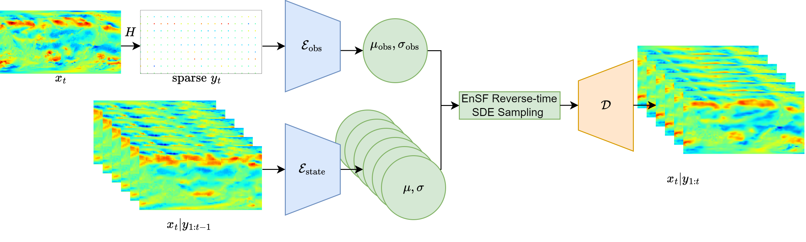
Figure 1: Flow of the Latent-EnSF. An ensemble of prior states $x_{t}|y_{1:t-1}$ is assimilated with sparse observation $y_{t}$ in the latent autoencoder space to obtain samples $x_{t}|y_{1:t}$ from the posterior.

We will begin by formally introducing data assimilation problems with a review of the EnSF in Section 2, follow up with how we integrate this with coupled variational autoencoders in Section 3 to create our Latent-EnSF, and finally conclude with experiments in Section 4.

2 Dynamical Systems and Data Assimilation

To model a dynamical physical system, we denote the state at a certain time $t$ as $x_{t}\in\mathbb{R}^{d}$, where $d$ is typically very high for complex models. For a system with discrete time steps $t=1,2,\dots$, given initial condition $x_{0}$, we then model the evolution of the state from the time $t-1$ to time $t$ as

$$x_{t}=M(x_{t-1},\varepsilon_{t}),$$ (1)

where $\varepsilon_{t}$ is a process noise term coming from a known distribution; this term accounts for hidden interactions and numerical errors. The corresponding observation $y_{t}\in\mathbb{R}^{m}$ at time $t$ is given by

$$y_{t}=H(x_{t})+\gamma_{t},$$ (2)

where $\gamma_{t}$ (also coming from a known distribution, typically Gaussian) represents the observation noise because of instrumental inaccuracies, etc. Both the model map $M:\mathbb{R}^{d}\times\mathbb{R}^{d}\to\mathbb{R}^{d}$ and the observation map $H:\mathbb{R}^{d}\to\mathbb{R}^{m}$ can be nonlinear.

Now, the model of the dynamical system in Equation 1 may lead to inaccurate representation of the ground truth with increasing discrepancy in time because of, e.g., model inadequacy or input uncertainty. The goal of data assimilation is to assimilate the observation data of the true state to the model of the dynamical system and recover an accurate representation of the true state. Note that in practical applications the observation data can be sparsely distributed in both space and time, which makes the recovery of the true state very challenging, especially for high dimensional problems with the state dimension $d\gg 1$, and the observation dimension $m$ much smaller than $d$.

2.1 Bayesian Filtering

From a Bayesian filtering perspective (Dore et al., 2009), a data assimilation problem at each time $t$ can be divided into two steps: a prediction step that advances the dynamical system and an update step that assimilates the data. Assuming that the posterior density of the state $x_{t-1}$ given observation data $y_{1:t-1}=(y_{1},\dots,y_{t-1})$, denoted as $P(x_{t-1}|y_{1:t-1})$, is available at time $t-1$, with $P(x_{0}|y_{1:0})=P(x_{0})$ given for time $t-1=0$, then the prediction step provides the density of $x_{t}$ as

$$\textbf{Prediction: }P(x_{t}|y_{1:t-1})=\int P(x_{t}|x_{t-1})P(x_{t-1}|y_{1:t-1})dx_{t-1},$$ (3)

where $P(x_{t}|x_{t-1})$ represents the transition probability governed by the dynamical system in Equation 1. Note that $x_{t}$ depends on $y_{1:t-1}$ only through $x_{t-1}$. Let $P(y_{t}|x_{t})$ denote the likelihood function of the data $y_{t}$ given state $x_{t}$ from Equation 2. Then, the update step provides the updated posterior density $P(x_{t}|y_{1:t})$ of the state $x_{t}$ given the new observation data $y_{t}$ by Bayes’ rule as

$$\textbf{Update: }P(x_{t}|y_{1:t})=\frac{P(y_{t}|x_{t})P(x_{t}|y_{1:t-1})}{P(y_{t}|y_{1:t-1})},$$ (4)

where the normalization constant or model evidence term $P(y_{t}|y_{1:t-1})$ is given by $P(y_{t}|y_{1:t-1})=\int P(y_{t}|x_{t})P(x_{t}|y_{1:t-1})dx_{t}$, which is typically intractable to compute.

2.2 Diffusion Models and the Ensemble Score Filter

A recent development for a new particle filter is the EnSF, where the ensemble of samples can be drawn from the posterior distribution through a diffusion process. It builds on the recent advancement in score-based generative modeling (Ho et al., 2020) in generating high-fidelity samples from a distribution by first computing a score function $\nabla_{x}P(x)$ and then sampling with it by solving stochastic differential equations (SDE) (Song et al., 2021). This circumvents knowing the true density as it only needs to generate samples from the posterior distribution. Notably, the diffusion model takes the form of a noisy forward stochastic differential equation process

$$dx=f(x,\tau)d\tau+g(\tau)dw,$$ (5)

which transforms data from an arbitrary distribution to an isotropic Gaussian for $\tau\in\mathcal{T}=[0,T]$. Here, $f(x,\tau)$ is a drift term, $g(\tau)$ is a diffusion term, and $w$ is a $d$-dimensional Wiener process. It has the corresponding reverse-time SDE that runs backward in time from $\tau=T$ to $0$ as

$$dx=[f(x,\tau)-g^{2}(\tau)\nabla_{x}\log P_{\tau}(x)]d\tau+g(\tau)d\bar{w},$$ (6)

where $\bar{w}$ is another Wiener process independent of $w$. This reverse-time SDE can be solved to sample from the distribution $P(x)$ if the score function $\nabla_{x}\log P(x_{\tau})$ is known, e.g., by the Euler–Maruyama scheme at the discrete time steps $0=\tau_{0}<\tau_{2}<...<\tau_{k}=T$.

In the following part, we use $x_{t,\tau}$ to indicate the state at physical time $t$ and diffusion time $\tau$. The EnSF method (Bao et al., 2024b) uses $T=1$ and the following drift and diffusion terms

$$f(x_{t,\tau},\tau)=\frac{d\log\alpha_{\tau}}{d\tau}x_{t,\tau}\text{ and }g^{2}(\tau)=\frac{d\beta_{\tau}^{2}}{d\tau}-2\frac{d\log\alpha_{\tau}}{d\tau}\beta_{\tau}^{2},$$ (7)

with $\alpha_{\tau}=1-\tau(1-\epsilon_{\alpha})$ and $\beta^{2}_{\tau}=\epsilon_{\beta}+\tau(1-\epsilon_{\beta})$ for two small positive hyperparameters $\epsilon_{\alpha}$ and $\epsilon_{\beta}$ which aid in avoiding the collapse of the generated samples. This choice leads to the distribution $x_{t,\tau}\sim N(\alpha_{\tau}x_{t,0},\beta^{2}_{\tau}I)$ conditioned on $x_{t,0}=x_{t}$, which results in the prior score function

$$\begin{split}\nabla_{x}\log P(x_{t,\tau}|y_{1:t-1})&=\nabla_{x}\log\int P(x_{t,\tau}|x_{t})P(x_{t}|y_{1:t-1})dx_{t}\\ &=\int-\frac{x_{t,\tau}-\alpha_{\tau}x_{t}}{\beta_{\tau}^{2}}\omega(x_{t,\tau},x_{t})P(x_{t}|y_{1:t-1})dx_{t},\end{split}$$ (8)

where the gradient $\nabla_{x}$ is taken with respect to $x_{t,\tau}$, and the weight $\omega(x_{t,\tau},x_{t})$ is given by

$$\omega(x_{t,\tau},x_{t})=\frac{P(x_{t,\tau}|x_{t})}{\int P(x_{t,\tau}|x_{t}^{\prime})P(x_{t}^{\prime}|y_{1:t-1})dx_{t}^{\prime}}.$$ (9)

Both the score function in Equation 8 and the weight in Equation 9 can be evaluated by sample average approximation with random samples from the distribution $P(x_{t}|y_{1:t-1})$ obtained in the prediction step in Equation 3. In the update step in Equation 4, the posterior score function in the EnSF method (Bao et al., 2024b) is formulated as

$$\nabla_{x}\log P(x_{t,\tau}|y_{1:t})=\nabla_{x}\log P(x_{t,\tau}|y_{1:t-1})+h(\tau)\nabla_{x}\log P(y_{t}|x_{t,\tau}),$$ (10)

with the prior score function in the first term given in Equation 8, the likelihood function $P(y_{t}|x_{t,\tau})$ in the second term given explicitly from the observation map in Equation 2, and a damping function $h(\tau)$ that is monotonically decreasing with $h(0)=1$ and $h(1)=0$, e.g., $h(\tau)=1-\tau$. Note that the posterior score function is consistent with the Bayes’ rule for the posterior in Equation 4 at $\tau=0$.

To this end, a brief description of one step of the EnSF algorithm is presented in Algorithm 1.

Algorithm 1 One Step of EnSF

Ensemble of the states $\{x_{t-1}\}$ from distribution $P(x_{t-1}|y_{1:t-1})$ and the observation $y_{t}$.

Ensemble of the states $\{x_{t}\}$ from the posterior distribution $P(x_{t}|y_{1:t})$.

Run the (stochastic) dynamical system model in Equation 1 from $\{x_{t-1}\}$ to obtain samples $\{x_{t}\}$.

for $\tau=\tau_{k},...,\tau_{0}$ do

     Estimate the prior score $\nabla_{x}\log P(x_{t,\tau}|y_{1:t-1})$ using Equation 8 and 9.

     Estimate the posterior score $\nabla_{x}\log P(x_{t,\tau}|y_{1:t})$ using Equation 10.

     Solve the reverse-time SDE in Equation 6 to generate the ensemble $\{x_{t}\}$.

end for

There are a number of advantages that EnSF provides over EnKF, particularly in high dimensions, where a much larger number of ensemble members are typically required for EnKF to have a good estimate of the approximate Gaussian density, while EnSF leverages the explicit likelihood function and the diffusion process to generate samples. In addition, EnSF does not assume approximate linearity of the dynamical system, making it highly applicable to high-dimensional and nonlinear filtering problems, e.g., a million-dimensional Lorenz-96 system (Bao et al., 2024b) and a surface quasigeostrophic model (Bao et al., 2024a). However, the key limitation of EnSF to filtering with sparse observation arises also from the explicit use of the likelihood function, as explained below.

2.3 Sparse Observations

A key limitation of EnSF in high-dimensional nonlinear filtering problems occurs when the observation data are sparse, which is the case for most practical applications. For example, suppose that the observation map $H(x_{t})=x_{t}[S]$, which only make observations of $x_{t}$ in the dimensions from the subset $S\subset\{1,...,d\}$, where $S$ may have a much smaller cardinality $|S|\ll d$ than the full dimension. In this case, the gradient of the log-likelihood $\nabla_{x}\log P(y_{t}|x_{t})$ vanishes in the dimensions in $\{1,...,d\}/S$, as shown in Figure 2, where we calculate $\nabla_{x}P(y_{t}|x_{t})$ for one of our experiments in Section 4.1 with 1/16 of the total dimensions used for the observations. Note that, the gradient is nonzero only at the points which are observed as seen in Figure 2. Though the ramifications are minimal for sufficiently dense observations, the vanishing gradients for higher sparsity scenarios significantly limits the effectiveness of the standard EnSF, which we demonstrate empirically in section 4.1.1.

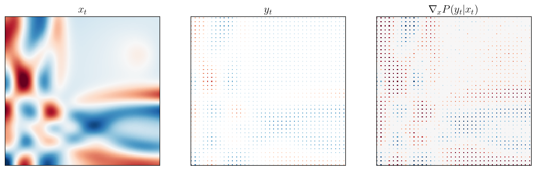
Figure 2: The gradient of the log-likelihood function $\nabla_{x}P(y_{t}|x_{t})$ (right) vanishes at the points where the sparse observation data $y_{t}$ (middle) do not have any information of the state $x_{t}$ (left).

To mitigate this weakness of the EnSF, rather than conducting data assimilation in the full state space with sparse observations, we propose to transform the data assimilation into a learned latent space with sufficiently preserved information and significantly reduced dimension.

3 Latent ensemble score filter

To address the key limitation of EnSF in the case of sparse observations due to the vanishing gradient of the log-likelihood function, we propose a latent representation of the sparse observations by a variational autoencoder (VAE) and match this latent representation to the encoded full state for the sake of consistent data assimilation in the latent space, for which we employ EnSF with the additional advantage of VAE regularization of the latent variables.

The advantages are twofold: it allows us to not only make use of the benefits of standard latent score-based generative models (Vahdat et al., 2021; Rombach et al., 2022) which offer optimized sampling speed and expressivity, but also create a expressive map from a sparse observation space to a full-dimensional latent space. Additionally, the successful application of latent-diffusion models to videos (Blattmann et al., 2023) offers a potential application of exploring latent-assimilation coupled with latent dynamics.

3.1 Compression by variational autoencoder

The Variational Autoencoder (VAE) (Kingma & Welling, 2014) provides a compressed representation of a high-dimensional distribution by means of bottlenecking. Note that since this is a family of models, it admits many specific instances such as VQ-VAE (Van Den Oord et al., 2017), InfoVAE (Zhao et al., 2019), etc., which can promote desirable properties such as independence and adaptable priors in the latent space. VAEs have two components, an encoder $\mathcal{E}$ and a decoder $\mathcal{D}$. The encoder casts the original state $x\in\mathbb{R}^{d}$ into a low dimensional representation $\mathcal{E}(x)\in\mathbb{R}^{2r}$ such that $2r\ll d$. Then, the model splits $\mathcal{E}(x)$ into mean $\mu\in{\mathbb{R}^{r}}$ and variance $\sigma^{2}\in{\mathbb{R}^{r}}$, and samples from the normal distribution $N(\mu,\Sigma)$ with $\Sigma=\text{diag}(\sigma_{1}^{2},\dots,\sigma_{r}^{2})$ by applying a reparameterization trick $z=\mu+\sigma\cdot\epsilon$, where $\epsilon\in N(0,I_{r})$. The decoder then constructs an approximation of the state as $\tilde{x}=\mathcal{D}(z)$.

VAEs are trained by optimizing for the evidence lower bound (ELBO), which is composed of a reconstruction term in the state space (e.g. the MSE $||x-\tilde{x}||_{2}^{2}$) and a Kullback–Leibler divergence (KLD) regularization term in the latent space, which is given by

$$\text{KLD}(\mu,\Sigma)=\sum_{i=1}^{r}-\log(\sigma_{i})+\frac{\sigma_{i}^{2}+\mu_{i}^{2}}{2}-\frac{1}{2},$$ (11)

which skews $N(\mu,\Sigma)$ to be close to $N(0,I_{r})$.

3.2 Coupled VAEs with Latent-Space Matching

We use VAEs to compress both the sparse observations and the full states to the latent space. To achieve consistent latent representations of sparse observations and full states, we couple the VAEs in the latent space as shown in Figure 3.

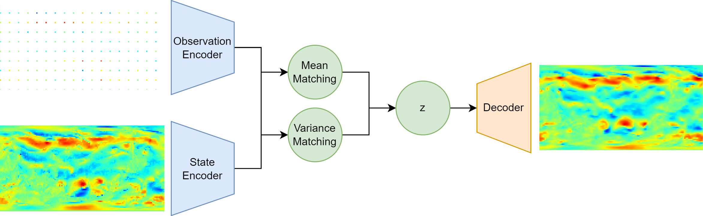
Figure 3: A coupled VAE for consistent latent representations of sparse observations and full states.

Specifically, we formulate a coupled VAE with two encoders, one encoder $\mathcal{E}:\mathbb{R}^{d}\rightarrow\mathbb{R}^{2r}$ that encodes the full state $x_{t}$ to a latent variable $z_{t}$ with distribution $N(\mu_{t},\Sigma_{t})$, where $(\mu_{t},\sigma^{2}_{t})=\mathcal{E}(x_{t})$, and $z_{t}=\mu_{t}+\sigma_{t}\cdot\epsilon_{t}$, and the other encoder $\mathcal{E}_{\text{obs}}:\mathbb{R}^{m}\rightarrow\mathbb{R}^{2r}$ that encodes the sparse observation $y_{t}$ to another latent variable $z_{t}^{\text{obs}}$ with distribution $N(\mu^{\text{obs}}_{t},\Sigma^{\text{obs}}_{t})$, where $(\mu^{\text{obs}}_{t},(\sigma_{t}^{\text{obs}})^{2})=\mathcal{E}_{\text{obs}}(y_{t})$ and $z_{t}^{\text{obs}}=\mu^{\text{obs}}_{t}+\sigma^{\text{obs}}_{t}\cdot\epsilon_{t}$. To assimilate the encoded latent data to the encoded latent state, we seek to match the two latent representations for their means and variances. To build a consistent reconstruction of the full state from the latent representation, we use the same decoder $\mathcal{D}:\mathbb{R}^{r}\to\mathbb{R}^{d}$. To this end, we formulate the following loss function to account for all three contributions:

$$\ell_{t}(\theta) =||x_{t}-\mathcal{D}(z_{t})||_{2}^{2}+||x_{t}-\mathcal{D}(z^{\text{obs}}_{t})||_{2}^{2}$$ (Reconstruction Term) (12)

$$+\text{KLD}(\mu_{t},\Sigma_{t})+\text{KLD}(\mu^{\text{obs}}_{t},\Sigma^{\text{obs}}_{t})$$ (Regularization Term) (13)

$$+||\mu_{t}-\mu^{\text{obs}}_{t}||_{2}^{2}+||\Sigma_{t}-\Sigma^{\text{obs}}_{t}||_{2}^{2} \text{ (Latent Matching Term)},$$ (14)

where $\theta$ represents the parameters of the encoders and decoder, for which we use convolutional neural networks (CNNs) in this work. Then for the training of the parameter $\theta$ in the coupled VAE, we minimize an empirical loss function as a sum of the above loss function over the training trajectories of the dynamical system, and over all the time steps $t$ in each trajectory.

Note that both of the latent representations use the same decoder for reconstruction of the full state. By training a coupled VAE which minimizes the error for the reconstruction of the true state conditioned on the observations, we can strive to obtain a latent representation of the sparse observations consistent to that of the full states. This approach is similar to the Generalized Latent Assimilation (GLA) representation proposed by Cheng et al. (2023), but with the addition of matching the means and variances of the state and observation encoders, as illustrated in Figure 3. Experimentally, training the encoders without matching the latent representations can lead to a solution where the latent observations are segregated from the latent states, yet result in sufficient reconstructions. Using these two separate encoders, we can match the latent representations such that we are able to apply EnSF in a full-dimensional manner, even with extremely sparse observations.

Some early papers have utilized autoencoder architectures to conduct data assimilation in various ways. GLA proposed in Cheng et al. (2023) uses the EnKF to assimilate observations in the latent space of the VAE. However, for latent spaces with high dimensions, EnKFs are computationally expensive and also subject to the curse of dimensionality. Meanwhile, overly constricting the latent dimension to simplify the computation would lead to magnified reconstruction errors, so the GLA algorithm needs to strike a balance between efficiency and accuracy. Additionally, depending on the type of architecture, local structures may be lost when encoding the state vector into the latent vector, so localized methods such as the LETKF (Hunt et al., 2007) can lose their advantage.

3.3 Latent ensemble score filter

For simplicity, let the latent state $\xi_{t}$ and latent data $\zeta_{t}$ be defined as the encoded state and data as

$$\xi_{t}=(\mu_{t},\sigma_{t}^{2})=\mathcal{E}(x_{t})\text{ and }\zeta_{t}=(\mu_{t}^{\text{obs}},(\sigma_{t}^{\text{obs}})^{2})=\mathcal{E}_{\text{obs}}(y_{t}),$$ (15)

respectively. We conduct data assimilation in the latent space by assimilating the latent data $\zeta_{t}$ to the latent state $\xi_{t}$. Mathematically, the latent state $\xi_{t}$ follows approximately (up to the VAE reconstruction error) the latent dynamical system

$$\xi_{t}\approx\mathcal{E}(M(\mathcal{D}(z_{t-1}(\xi_{t-1})),\varepsilon_{t}))$$ (16)

as a result of the full dynamical system in Equation 1 and the VAE with the reparametrization $z_{t-1}(\xi_{t-1})=\mu_{t-1}+\sigma_{t-1}\cdot\epsilon_{t-1}$ at time $t-1$. The latent data $\zeta_{t}$ approximately satisfies

$$\zeta_{t}=\mathcal{E}_{\text{obs}}(H(\mathcal{D}(z_{t}(\xi_{t}))+\gamma_{t})$$ (17)

as a result of the observation map in Equation 2 and the VAE with the reparametrization $z_{t}(\xi_{t})=\mu_{t}+\sigma_{t}\cdot\epsilon_{t}$ at time $t$. When calculating the likelihood of the observation in the latent space, we can simply Equation 17 and use an additive latent observation noise $\hat{\gamma}_{t}$ estimated from the full space observation noise $\gamma_{t}$ through the observation encoder. As the coupled encoders seek to match the full states and the sparse observations in their latent representations, we can further approximate the latent observation map in Equation 17 as an identity map, i.e., $\zeta_{t}\approx\xi_{t}+\hat{\gamma}_{t}$, which simplifies and accelerates the computation of the gradient of the log-likelihood function by avoiding automatic differentiation through the map in Equation 17 with respect to the latent state.

With the latent state following the latent dynamics, and the approximate latent observations, we consider the Bayesian filtering problem in the latent space by formulating the prediction step as

$$\textbf{Prediction: }P(\xi_{t}|\zeta_{1:t-1})=\int P(\xi_{t}|\xi_{t-1})P(\xi_{t-1}|\zeta_{1:t-1})d\xi_{t-1},$$ (18)

with the transition probability $P(\xi_{t}|\xi_{t-1})$ detemined by the latent dynamical system in Equation 16. The update step for the posterior of the latent state $\xi_{t}$ given the latent data $\zeta_{t}$ is defined as

$$\textbf{Update: }P(\xi_{t}|\zeta_{1:t})=\frac{P(\zeta_{t}|\xi_{t})P(\xi_{t}|\zeta_{1:t-1})}{P(\zeta_{t}|\zeta_{1:t-1})},$$ (19)

where $P(\zeta_{t}|\xi_{t})$ is the likelihood of the latent data given latent state $\xi_{t}$, which can be computed by the latent observation map in Equation 17. The latent normalization term $P(\zeta_{t}|\zeta_{1:t-1})=\int P(\zeta_{t}|\xi_{t})P(\xi_{t}|\zeta_{1:t-1})d\xi_{t}$ is also generally intractable.

We employ the diffusion-based ensemble score filter in Section 2.2 for the above Bayesian filtering problem in the latent space by replacing the state $x_{t}$ with the latent state $\xi_{t}$, and the observation $y_{t}$ with the latent observation $\zeta_{t}$. Note that the latent state $\xi_{t}$ and the latent observation $\zeta_{t}$ have the same dimension $2r\ll d$. We present one step of the Latent-EnSF in Algorithm 2.

Algorithm 2 One Step of Latent EnSF

Ensemble of the states $\{x_{t-1}\}$ from distribution $P(x_{t-1}|y_{1:t-1})$ and the observation $y_{t}$. State encoder $\mathcal{E}$, observation encoder $\mathcal{E}_{\text{obs}}$, and decoder $\mathcal{D}$.

Ensemble of the states $\{x_{t}\}$ from the posterior distribution $P(x_{t}|y_{1:t})$.

Encode the state $\xi_{t-1}=\mathcal{E}(x_{t-1})$ and the observation $\zeta_{t}=\mathcal{E}_{\text{obs}}(y_{t})$.

Run the (stochastic) dynamical system model in Equation 16 from $\{\xi_{t-1}\}$ to obtain samples $\{\xi_{t}\}$.

for $\tau=\tau_{k},...,\tau_{0}$ do

     Estimate the prior score $\nabla_{\xi}\log P(\xi_{t,\tau}|\zeta_{1:t-1})$ using Equation 8 and 9 in the latent space.

     Estimate the posterior score $\nabla_{\xi}\log P(\xi_{t,\tau}|\zeta_{1:t})$ using Equation 10 in the latent space.

     Solve the reverse-time SDE in Equation 6 to generate the ensemble of latent states $\{\xi_{t}\}$.

end for

Sample $z_{t}=\mu_{t}+\sigma_{t}\cdot\epsilon_{t}$ from the ensemble of the latent states $\xi_{t}=(\mu_{t},\sigma_{t})$ and samples of $\epsilon_{t}$.

Decode the ensemble of latent variables $\{z_{t}\}$ to the ensemble of the full states by $x_{t}=\mathcal{D}(z_{t})$.

Because the sparse observations have been mapped to the same dimension as the state in the latent space, we are able to circumvent the weakness of the EnSF with vanishing gradient of the log-likelihood function when dealing with the sparse observation problems. In addition, since the encoder is a flexible neural-network representation, the model is able to restrict the latent observation map $H_{\text{latent}}$ in the latent space to be the identity function $H_{\text{latent}}(\xi_{t})=\xi_{t}$, allowing for analytical solutions for the score function without the need for automatic differentiation. This means that the model can leverage the full computational speed-up of the EnSF in the latent space. Finally, the regularization done by the VAE such that the latent vector tends to follow a $N(0,1)$ distribution simplifies hyperparameter search of the appropriate noise $\gamma_{t}$ for real world problems.

3.4 Addressing EnSF’s numerical instability on small scales

In practice, when applying the EnSF to problems where the values of the states and their variances are very small, specifying the corresponding observation noise such that $\gamma_{t}\ll 0.05$ can result in numerical instability issues when sampling the posterior distribution by reverse time SDE with the drift and diffusion terms given in Equation 7.

This numerical instability issue is also present in the VAE latent space where the components are regularized such that $\mu_{t}\approx 0$ and $\sigma_{t}\approx 1$. We address this issue by multiplying the latent representations with a scalar constant $\psi_{\text{latent}}$, conducting the EnSF for the rescaled latent representation, and subsequently scaling the posterior samples back to the original latent representation. We conducted a small grid search experiment when working with the shallow water wave propogation problem in Section 4.1, where $\psi_{\text{latent}}=500$ seemed to work reasonably.

Remarkably, this $\psi_{\text{latent}}$ applies well in all our experiments, which implies that this scaling hyperparameter stays fairly steady across all problems. Intuitively, this is consistent; the latent regularization conducted by the VAE constrains the latent space to be in a similar range. In contrast, when EnSF is conducted on the full state space, such advantages are lost and a different scaling parameter $\psi$ is needed for different problems with different scales of the state and observation noise.

4 Experiments

In this section, we illustrate the limitation of using the EnSF for sparse observations, and demonstrate the improved accuracy and fast convergence of the Latent-EnSF compared to several data assimilation methods for a synthetic complex physical system modeled by shallow water equations with sparse observations in both space and time. We also demonstrate the merits of Latent-EnSF for medium-range weather forecasting with real-world data and a ML-based dynamical system.

4.1 Shallow water wave propagation

We consider the propagation of shallow water waves described by shallow-water equations (Vreugdenhil, 1994), which are a system of hyperbolic PDEs that describe fluid flow of free surface with the conservation of momentum and mass, with three state variables including the water height and two components of the water velocity field. Such models find practical applications in hydrology for predicting flood waves and in oceanography for modeling tsunami wave propagation.

In the experiment, we consider water wave propagation with the initial water displacement modeled by a local Gaussian bump perturbation from the flat surface in a square domain of size $L\times L$ with $L=10^{6}$ m in each direction and a constant depth $h=100$ m for the topography of the floor. For the simulation, we use a finite difference code adapted from jostbr (2019), with the domain discretized into a uniform grid of $150\times 150$. The simulation is then run for 2000 time steps using a upwind scheme with a time step $\Delta t=0.1\frac{\Delta x}{\sqrt{gh}}$ with $\Delta x=L/150$ to satisfy the Courant–Friedrichs–Lewy condition (Courant et al., 1967), see Figure 5 for the evolution of the height and its sparse observations with 4x ($75\times 75$) and 225x ($10\times 10$) data reduction.

For the data assimilation, we start with a mis-estimated initial state where the Gaussian bump perturbation is shifted away from the true initial state. 100 ensemble members are then taken by adding a negligible amount of noise to the mis-estimated state. The data assimilation is conducted with observations every 20 time steps unless otherwise stated, for a total of 100 assimilation steps, with an observation noise variance of 1. When conducting the EnSF, we take 100 forward Euler steps to solve the reverse-time SDE, and use hyperparameters $\epsilon_{\alpha}=0.05$, $\epsilon_{\beta}=0$.

4.1.1 EnSF and Sparsity

In Section 2.3, we illustrated the vanishing gradient of the log-likelihood function for the dimensions in which observations are not available. Here we empirically demonstrate this effect on EnSF for data assimilation with sparse observations at different levels of sparsity.

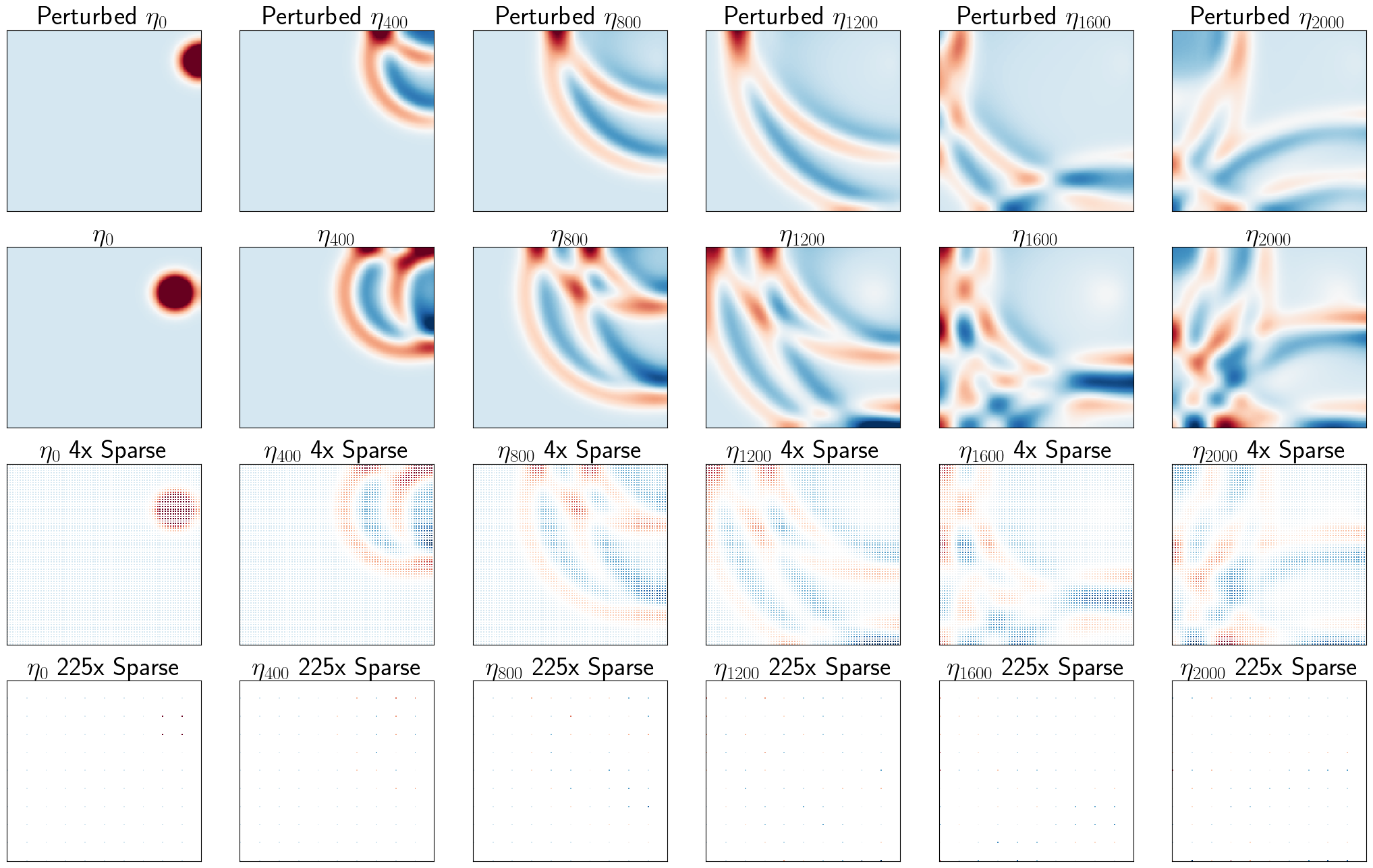
Figure 4: Evolution of states and sparse observations.

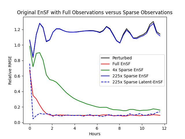
Figure 5: Relative RMSE of EnSF and Latent-EnSF for sparse observations.

In Figure 5, we plot the performance in terms of relative root mean square error (RMSE) of the assimilated state as the observation space becomes increasingly sparse. The relative error of the perturbed trajectory and the original trajectory is also plotted as a reference. We can observe that when using the EnSF, increasing the sparsity of the observation data leads to increasing assimilation errors and slower convergence to the true state. In particular, for extreme cases such as when the observation data are reduced by a factor of 225 times, there is almost no discernible difference between the assimilated error of EnSF compared to a non-assimilated trajectory, or EnSF does not bring any improvement in the data assimilation. In contrast, the Latent-EnSF achieves small relative errors with fast convergence to the true state even in the case of extreme sparsity, with the errors at the same level achieved by EnSF with the observation of the full state. These findings align with Bao et al. (2024a) where the sparsity in their experiments for EnSF is limited to a 2x reduction.

4.1.2 Latent-EnSF Results

We train the coupled VAE as shown in Figure 3 using convolutional layers with input dimension $3\times 150\times 150$ and latent dimension $4\times 10\times 10=400$ with 4 channels for the experiments other than that in Figure 6, which is for the evaluation of the performance with respect to the latent dimension size. The following experiments use a $10\times 10$ observation grid, corresponding to the 225x sparse entry in Figure 5. We compare the Latent-EnSF and the Latent-EnKF, which shares the same VAE weights as the Latent-EnSF. For the approximate $\gamma_{t}$ observation noise terms in the latent space, we adopt a heuristic by taking the mean standard deviation values given by encoded latent states for all three approaches. In Figure 6, we can see that the Latent-EnKF struggles with higher dimensional latent spaces, whereas the Latent-EnSF gets more accurate as a result of a decrease in reconstruction error for the VAE, even though they perform similarly for the 100-dimensional case.

In addition to the Latent-EnKF, we test against the Latent-LETKF in high-dimensional latent space, as shown in the right part of Figure 6. This utilizes the LETKF which in practice handles high-dimensional data assimilation much better than the EnKF. However, we can see that though it indeed beats the Latent-EnKF benchmark, especially with higher latent dimensions, our approach is still much better in terms of assimilation speed, accuracy, and efficiency (see Table 1) for all cases.

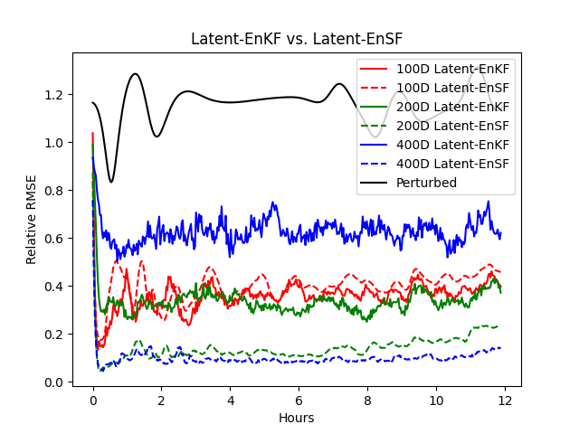
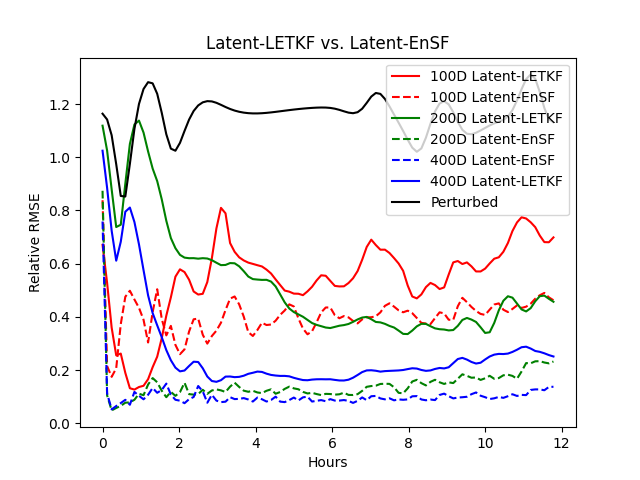
Figure 6: Relative RMSE of Latent-EnSF compared to Latent-EnKF (left) and Latent-LETKF (right) with varying latent dimensions, with the error of the perturbed state shown as a reference.

Figure 7 shows the comparison of the assimilated results of sparse observations using different methods at the first time step, time step 1000, and 2000 (the final time step). We can observe that even though the perturbed dynamics is very far from the ground truth, the Latent-EnSF is able to push the perturbed dynamics to match the ground truth very well with small error, while EnSF fails to do so with its error very close to the difference between the perturbed and true states. Moreover, Latent-EnSF performs the best among the data assimilation methods in the same latent space.

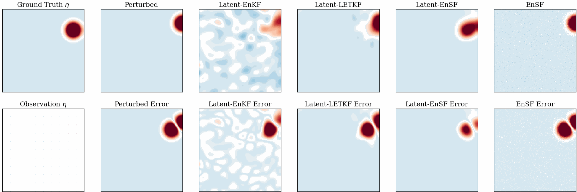
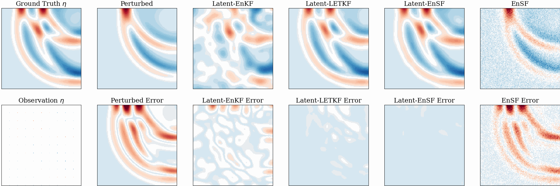
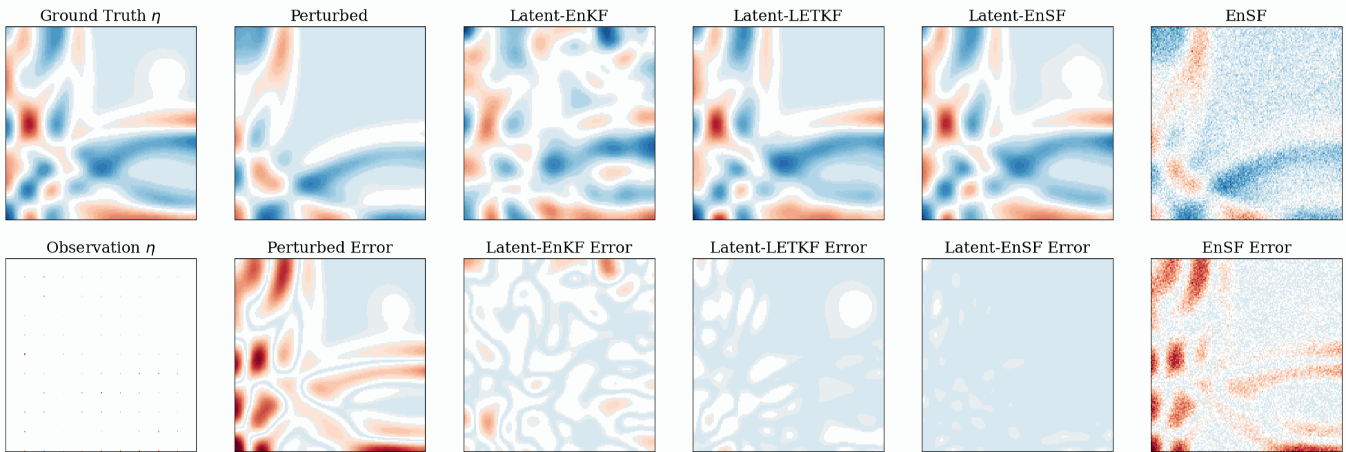
Figure 7: Comparison of different methods at time step 1 (top two rows), 1000 (middle two rows), and 2000 (bottom two rows), with the ground truth, perturbed states, and assimilated states on the top and their corresponding errors from the ground truth at the bottom of each two rows.

In Figure 8, we report the comparison of Latent-EnSF and Latent-LETKF for their performances with different temporal sparsity in the observations, which come in every 5, 20, and 50 time steps with increasing sparsity. As we can observe, the assimilation accuracy of Latent-EnSF is not affected by the increased sparsity; only the burn-in time is slightly increased. In contrast, the Latent-LETKF is very sensitive to the temporal sparsity, with much slower convergence for larger sparsity, while Latent-EnSF is robust to sparse observations not only in space but also in time in this experiment.

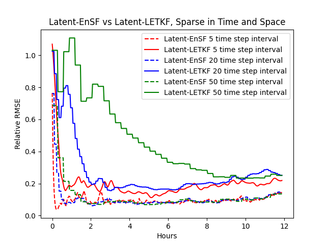
Figure 8: Relative RMSE of Latent-EnSF vs Latent-LETKF for varying observation sparsity in time, with the assimilation frequency at every 5, 20, and 50 time steps, respectively.

4.2 Medium-Range Weather Forecasting

Sparse data assimilation is particularly important for accurate medium-range weather forecasting due to the complexity of the problem which can skew results of machine learning models. The commonly used dataset for conducting these weather forecasting experiments is the ERA5 (Hersbach et al., 2020), coming from the European Centre for Medium-Range Weather Forecasts (EMCWF). The main variables at play in this dataset include the wind speeds, temperature, geopotential, and humidity, just to name a few, all of which are available at any of the 137 different pressure levels. This dataset comes with 40 years of reanalyzed data, and can support various degrees of fidelity. Currently, ML-based prediction approaches such as FourCastNet (Pathak et al., 2022), Pangu Weather (Bi et al., 2023), and GraphCast (Lam et al., 2023) have shown to be extremely efficient when applied to weather forecasting compared to standard PDE-based approaches. We adopt the 21 variables used in the FourCastNet paper which include wind velocities and geopotential at 3 different pressure levels, along with relative humidity and temperature at a few key pressure levels and the total column water vapor at the surface. For forecasting, we train a FourCastNet model on our coarse subset of the dataset. When training the VAE for data assimilation, we create a ResNet-style architecture similar to what we constructed in the shallow-water experiments. The encoder downsamples by a factor of 2 twice between convolution layers, resulting in a latent dimension size of $32\times 36\times 18=20736$. In between the layers we use Leaky-ReLU layers with a coefficient of 0.2. We use this as a demonstrative task to show the feasibility of applying Latent-EnSF to complex systems, so we train and test on 10 years of data with $2.5^{\circ}$ resolution, with a grid of size $144\times 72$, as a proof of concept. Evaluations are done for the year 2015, where we average the metrics across nine 41-day windows. Data assimilation is done once a day, incorporating observations at a 64x sparsity rate, with 8x reduction in each dimension, or a grid of $18\times 9$ observations.

As shown in Figure 9, the forecasting by the FourCastNet-based ML model without data assimilation becomes increasingly inaccurate because of the accumulated errors, which limits its relatively reliable prediction for the first 14 days. The data assimilation errors by EnSF follow closely those of FourCastNet forecasting without data assimilation, which implies that EnSF fails with the data assimilation with sparse observations. In contrast, the Latent-EnSF approach quickly levels off the error in the first couple of days and preserves the accuracy for all the following days, despite the increasing inaccuracy of the FourCastNet forecasting. Note that the Latent-LETKF leads to increasing assimilation errors, much higher than Latent-EnSF, with increasingly inaccurate FourCastNet forecasting. To demonstrate that the FourCastNet is helpful in the data assimilation, we also run the Latent-EnSF without a known dynamical model, in which case we assume the dynamics of the state does not evolve, i.e., $x_{t+1}=M(x_{t})=x_{t}$. From the comparison of Latent-EnSF No Model and Latent-EnSF (with FourCastNet), we observe that the ML-based FourCastNet forecasting does help for the data assimilation, even though it becomes increasingly inaccurate in the long run.

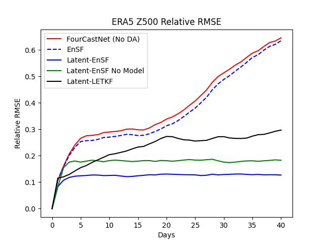
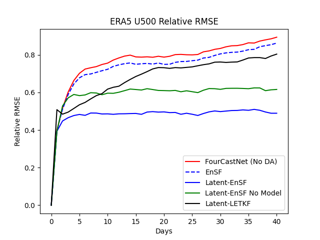
Figure 9: Relative RMSE for the assimilation of Z500 (geopotential at 500hPA) and U500 (u-component of wind at 500hPA) on the ERA5 with respect to the number of days of forecasting.

We observe in Figure 9 that the assimilation for the state Z500 is much more accurate than that of U500, which can also be observed in Figure 10 after 41 days of forecasting by FourCastNet and by data assimilation. This is due to the much higher state complexity with rich local characteristics and sharp changes in the u-component of the wind velocity U500, which would demand more data (with less sparsity) beyond the very sparse $18\times 9$ observations for more accurate data assimilation.

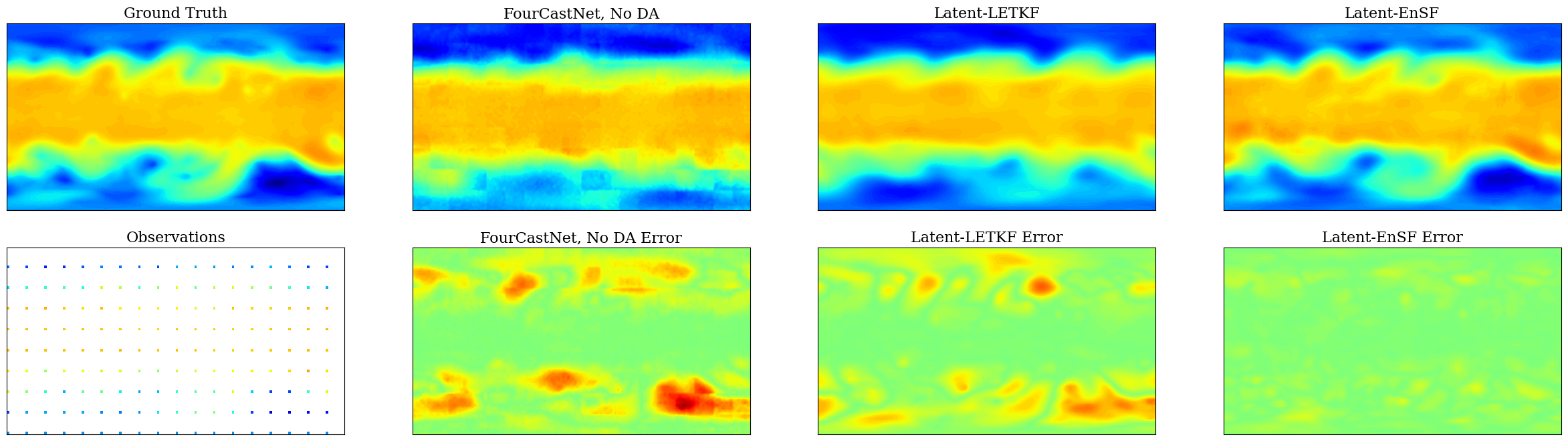
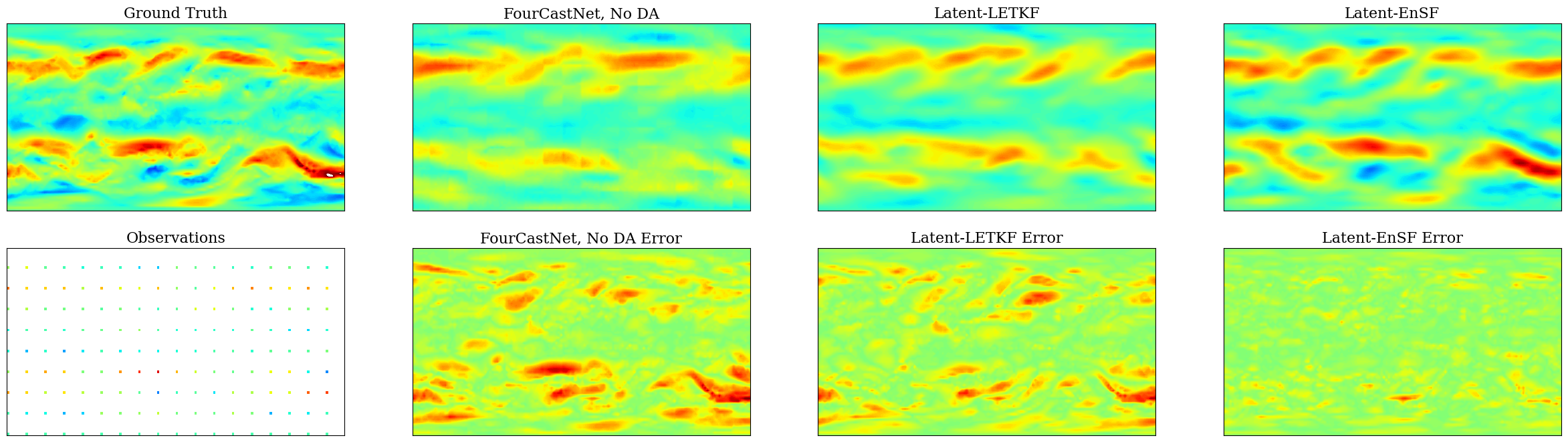
Figure 10: ERA5 Z500 (top two rows) and U500 (bottom two rows) medium-ranged weather forecasting samples after 41 days, along with the errors. Data assimilation is conducted once a day with 64x sparse observations. We compare against a baseline FourCastNet model and Latent-LETKF.

To examine the computational efficiency, we report the mean and standard deviation of the time it takes the same machine (a combination of an Nvidia A6000 GPU with an AMD 7543 CPU) for one step of the assimilation by each of the methods in Table 1 for the two applications. The latent dimension $2r$ is applicable to all methods except EnSF with dimension $d$ in the full space. We can see that even though the Latent-LETKF leads to higher accuracy than Latent-EnKF, it takes much more time than all the other methods, due to the need to iterate through the dimensions to construct each individual localization matrix (this could be ameliorated by parallel computing in many processors). However, the computational cost increases approximately linearly with respect to the dimensions compared to the much faster increase of the Latent-EnKF. In comparison, the Latent-EnSF achieves the highest accuracy, fastest convergence, and still uses the smallest time. By comparison of the two applications, we see that although the latent dimensions differ by a scale of 50, the Latent-EnKF takes over 700 times as long for assimilation in the higher latent dimension, compared to 68 times for Latent-LETKF and only 4 times for Latent-EnSF, which implies the much better scalability of the Latent-EnSF compared to the other methods. Additionally, note that even with the added complexity of doing a forward pass through the encoder and decoder, the assimilation by Latent-EnSF is still faster than that by EnSF in the full space, making Latent-EnSF highly conducive for real-time data assimilation.

Table 1: Mean and standard deviation of wall-clock time in seconds of different assimilation approaches for both our experiments, obtained using Nvidia A6000 GPU + AMD 7543 CPU.

Dataset	Latent Dim	Latent-EnKF	Latent-LETKF	Latent-EnSF	EnSF
SWE	400	$0.056\pm 0.002$	$6.567\pm 0.069$	$0.051\pm 0.001$	$0.223\pm 0.002$
ERA5	20736	$41.161\pm 0.640$	$450.213\pm 3.512$	$0.198\pm 0.008$	$0.501\pm 0.001$

5 Conclusion

In this paper, we introduced Latent-EnSF, a novel data assimilation method in addressing the joint challenges of high dimensionality in the state and high sparsity in the observation for nonlinear Bayesian filtering problems, which have been the key and common challenges for the existing approaches. We proposed a coupled VAE for information compression to the latent space, which is trained for a consistent match of the full states and sparse observations for their latent representations and with latent regularization, as well as for a consistent reconstruction of the full states. We also presented the corresponding approximate latent dynamical system and the simplified latent observation map in accelerating the sampling process in the latent space. We demonstrated the high accuracy, fast convergence, and high efficiency of the proposed method compared to other approaches for a challenging data assimilation problem with PDE-based shallow water wave propagation model and synthetic data that is sparse in both space and time. We also applied and demonstrated the advantage of the proposed method to a ML-based model with real-world data for data assimilation in medium-range weather forecasting.

For further avenues of interest, extending Latent-EnSF to incorporate latent dynamics could further enhance the computational efficiency. Additionally, exploring more complex architectures could allow us to conduct data assimilation for unstructured observation points and continuous-time data where extremely sparse observations arrive in a stochastic manner. Overall, Latent-EnSF presents a promising direction for advancing data assimilation techniques and bringing an efficient way of utilizing machine learning models to simulate real-world systems with improved accuracy.

References

- Asch et al. (2016) Mark Asch, Marc Bocquet, and Maëlle Nodet. Data Assimilation. Society for Industrial and Applied Mathematics, Philadelphia, PA, 2016. doi: 10.1137/1.9781611974546. URL https://epubs.siam.org/doi/abs/10.1137/1.9781611974546.
- Bao et al. (2024a) Feng Bao, Hristo G. Chipilski, Siming Liang, Guannan Zhang, and Jeffrey S. Whitaker. Nonlinear ensemble filtering with diffusion models: Application to the surface quasi-geostrophic dynamics, 2024a. URL https://arxiv.org/abs/2404.00844.
- Bao et al. (2024b) Feng Bao, Zezhong Zhang, and Guannan Zhang. An ensemble score filter for tracking high-dimensional nonlinear dynamical systems, 2024b. URL https://arxiv.org/abs/2309.00983.
- Bi et al. (2023) Kaifeng Bi, Lingxi Xie, Hengheng Zhang, Xin Chen, Xiaotao Gu, and Qi Tian. Accurate medium-range global weather forecasting with 3d neural networks. Nature, 619(7970):533–538, 2023.
- Bishop et al. (2001) Craig H. Bishop, Brian J. Etherton, and Sharanya J. Majumdar. Adaptive sampling with the ensemble transform kalman filter. part i: Theoretical aspects. Monthly Weather Review, 129(3):420 – 436, 2001. doi: 10.1175/1520-0493(2001)129¡0420:ASWTET¿2.0.CO;2. URL https://journals.ametsoc.org/view/journals/mwre/129/3/1520-0493_2001_129_0420_aswtet_2.0.co_2.xml.
- Blattmann et al. (2023) Andreas Blattmann, Robin Rombach, Huan Ling, Tim Dockhorn, Seung Wook Kim, Sanja Fidler, and Karsten Kreis. Align your latents: High-resolution video synthesis with latent diffusion models. In Proceedings of the IEEE/CVF Conference on Computer Vision and Pattern Recognition (CVPR), pp. 22563–22575, June 2023.
- Cheng et al. (2023) Sibo Cheng, Jianhua Chen, Charitos Anastasiou, Panagiota Angeli, Omar K Matar, Yi-Ke Guo, Christopher C Pain, and Rossella Arcucci. Generalised latent assimilation in heterogeneous reduced spaces with machine learning surrogate models. Journal of Scientific Computing, 94(1):11, 2023.
- Courant et al. (1967) R. Courant, K. Friedrichs, and H. Lewy. On the partial difference equations of mathematical physics. IBM J. Res. Dev., 11(2):215–234, mar 1967. ISSN 0018-8646. doi: 10.1147/rd.112.0215. URL https://doi.org/10.1147/rd.112.0215.
- Dore et al. (2009) Alessio Dore, Matteo Pinasco, and Carlo S. Regazzoni. Chapter 9 - multi-modal data fusion techniques and applications. In Hamid Aghajan and Andrea Cavallaro (eds.), Multi-Camera Networks, pp. 213–237. Academic Press, Oxford, 2009. ISBN 978-0-12-374633-7. doi: https://doi.org/10.1016/B978-0-12-374633-7.00011-2. URL https://www.sciencedirect.com/science/article/pii/B9780123746337000112.
- Hersbach et al. (2020) Hans Hersbach, Bill Bell, Paul Berrisford, Shoji Hirahara, András Horányi, Joaquín Muñoz-Sabater, Julien Nicolas, Carole Peubey, Raluca Radu, Dinand Schepers, Adrian Simmons, Cornel Soci, Saleh Abdalla, Xavier Abellan, Gianpaolo Balsamo, Peter Bechtold, Gionata Biavati, Jean Bidlot, Massimo Bonavita, Giovanna De Chiara, Per Dahlgren, Dick Dee, Michail Diamantakis, Rossana Dragani, Johannes Flemming, Richard Forbes, Manuel Fuentes, Alan Geer, Leo Haimberger, Sean Healy, Robin J. Hogan, Elías Hólm, Marta Janisková, Sarah Keeley, Patrick Laloyaux, Philippe Lopez, Cristina Lupu, Gabor Radnoti, Patricia de Rosnay, Iryna Rozum, Freja Vamborg, Sebastien Villaume, and Jean-Noël Thépaut. The era5 global reanalysis. Quarterly Journal of the Royal Meteorological Society, 146(730):1999–2049, 2020. doi: https://doi.org/10.1002/qj.3803. URL https://rmets.onlinelibrary.wiley.com/doi/abs/10.1002/qj.3803.
- Ho et al. (2020) Jonathan Ho, Ajay Jain, and Pieter Abbeel. Denoising diffusion probabilistic models. Advances in Neural Information Processing Systems, 33:6840–6851, 2020.
- Huang et al. (2024) Langwen Huang, Lukas Gianinazzi, Yuejiang Yu, Peter D. Dueben, and Torsten Hoefler. Diffda: a diffusion model for weather-scale data assimilation, 2024. URL https://arxiv.org/abs/2401.05932.
- Hunt et al. (2007) Brian R. Hunt, Eric J. Kostelich, and Istvan Szunyogh. Efficient data assimilation for spatiotemporal chaos: A local ensemble transform kalman filter. Physica D: Nonlinear Phenomena, 230(1):112–126, 2007. ISSN 0167-2789. doi: https://doi.org/10.1016/j.physd.2006.11.008. URL https://www.sciencedirect.com/science/article/pii/S0167278906004647. Data Assimilation.
- jostbr (2019) jostbr. shallow-water. https://github.com/jostbr/shallow-water, 2019.
- Kalman (1960a) R. E. Kalman. A New Approach to Linear Filtering and Prediction Problems. Journal of Basic Engineering, 82(1):35–45, 03 1960a. ISSN 0021-9223. doi: 10.1115/1.3662552. URL https://doi.org/10.1115/1.3662552.
- Kalman (1960b) Rudolph Emil Kalman. A new approach to linear filtering and prediction problems. Transactions of the ASME–Journal of Basic Engineering, 82(Series D):35–45, 1960b.
- Kingma & Welling (2014) Diederik P Kingma and Max Welling. Auto-encoding variational bayes. International Conference on Learning Representations, 2014.
- Künsch (2013) Hans R. Künsch. Particle filters. Bernoulli, 19(4), September 2013. ISSN 1350-7265. doi: 10.3150/12-bejsp07. URL http://dx.doi.org/10.3150/12-BEJSP07.
- Lam et al. (2023) Remi Lam, Alvaro Sanchez-Gonzalez, Matthew Willson, Peter Wirnsberger, Meire Fortunato, Ferran Alet, Suman Ravuri, Timo Ewalds, Zach Eaton-Rosen, Weihua Hu, et al. Learning skillful medium-range global weather forecasting. Science, 382(6677):1416–1421, 2023.
- Pathak et al. (2022) Jaideep Pathak, Shashank Subramanian, Peter Harrington, Sanjeev Raja, Ashesh Chattopadhyay, Morteza Mardani, Thorsten Kurth, David Hall, Zongyi Li, Kamyar Azizzadenesheli, Pedram Hassanzadeh, Karthik Kashinath, and Animashree Anandkumar. Fourcastnet: A global data-driven high-resolution weather model using adaptive fourier neural operators, 2022. URL https://arxiv.org/abs/2202.11214.
- Rabier & Liu (2003) Florence Rabier and Zhiquan Liu. Variational data assimilation: theory and overview. In Proc. ECMWF Seminar on Recent Developments in Data Assimilation for Atmosphere and Ocean, Reading, UK, September 8–12, pp. 29–43, 2003.
- Rombach et al. (2022) Robin Rombach, Andreas Blattmann, Dominik Lorenz, Patrick Esser, and Björn Ommer. High-resolution image synthesis with latent diffusion models. In Proceedings of the IEEE/CVF Conference on Computer Vision and Pattern Recognition (CVPR), pp. 10684–10695, June 2022.
- Sanz-Alonso et al. (2023) Daniel Sanz-Alonso, Andrew Stuart, and Armeen Taeb. Inverse problems and data assimilation, volume 107. Cambridge University Press, 2023.
- Song et al. (2021) Yang Song, Jascha Sohl-Dickstein, Diederik P. Kingma, Abhishek Kumar, Stefano Ermon, and Ben Poole. Score-based generative modeling through stochastic differential equations, 2021. URL https://arxiv.org/abs/2011.13456.
- Vahdat et al. (2021) Arash Vahdat, Karsten Kreis, and Jan Kautz. Score-based generative modeling in latent space. In M. Ranzato, A. Beygelzimer, Y. Dauphin, P.S. Liang, and J. Wortman Vaughan (eds.), Advances in Neural Information Processing Systems, volume 34, pp. 11287–11302. Curran Associates, Inc., 2021. URL https://proceedings.neurips.cc/paper_files/paper/2021/file/5dca4c6b9e244d24a30b4c45601d9720-Paper.pdf.
- Van Den Oord et al. (2017) Aaron Van Den Oord, Oriol Vinyals, et al. Neural discrete representation learning. Advances in neural information processing systems, 30, 2017.
- Vreugdenhil (1994) C.B. Vreugdenhil. Numerical Methods for Shallow-Water Flow. Water Science and Technology Library. Springer Netherlands, 1994. ISBN 9780792331643. URL https://books.google.com/books?id=8uohwO1mgaEC.
- Zhao et al. (2019) Shengjia Zhao, Jiaming Song, and Stefano Ermon. Infovae: Balancing learning and inference in variational autoencoders. In Proceedings of the aaai conference on artificial intelligence, volume 33, pp. 5885–5892, 2019.