Fast and Efficient Estimation of Resonant Modes: A Case Study of Mechanical Drivelines*
Abstract
This work presents the development of an online parameter estimation algorithm for the identification of resonating modes in a linear system of arbitrary order. The method employs a short-time Fourier transform of the input and output signals and uses a recursive least square (RLS) algorithm to detect resonant frequencies and damping factors of the resonant modes.
I Problem Statement
Consider a SISO linear time-invariant system with resonant modes described by the frequency response . The input and output signals are related through the following equation
| (1) |
where and are, respectively, the discrete Fourier transform (DFT) of the input and output signals.
Our objective is to determine the damping factors and resonant frequencies of the system by identifying the resonating poles of . This task can be simplified by assuming that around each resonant frequency, the behavior of the system is mainly dominated by the complex-conjugate poles. That is, can be approximated by
| (2) |
where is a constant complex number representing the effect of other terms in the frequency response at frequency . The parameters and depend on the resonant frequency and the damping factor.
The resonant frequency, , and the damping factor, , are then readily calculated by
| (3) |
Plugging in the reduced order model of , and splitting the signals into real and imaginary parts, lead to
| (4) |
where , , and are, respectively, the real and imaginary parts of the output and the input DFTs at frequency .
Eq. 4 can be split into real and imaginary parts and reformulated as follows
| (5) |
where is the parameter vector defined as
The Eq. 5 is in the form of , where and both depend on the frequency, whereas is a constant parameter vector. Therefore, the parameter vector, , can be estimated using a computationally efficient recursive least square (RLS) approach. The RLS algorithm is only applied only around the resonant frequency (for example within 20% bound of the initial guess), and recursively updates the estimated parameter according to the following set of equations,
| (6) |
where subscript captures the index of the DFT frequency points used for the estimation, and the matrix is the optimal gain matrix derived by the following equation
| (7) |
where is the covariance matrix on the , and is the covariance matrix of the estimate given by,
| (8) |
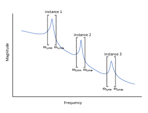
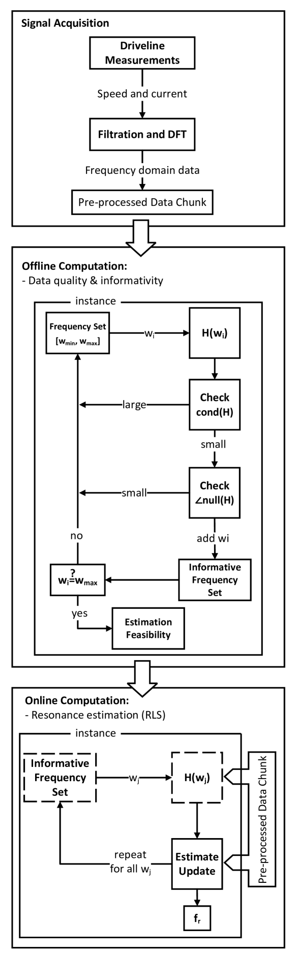
The resonant frequency and the damping factor are then computed online according to Eq. 3. For the case where multiple resonant modes are required to be estimated, the estimation schemes can be run in parallel instances (see Fig. 1), independent of one another, if the modes are distant.
II Case study: Mechanical driveline torsional vibration
Torsional vibrations in mechanical rotating drivelines cause gear wear that eventually leads to reduced performance at best and even shaft breakage and system failure. To avoid these issues, it is necessary to analyze the torsional response characteristics of the system to diagnose malfunctioning and employ preventive measures. The magnitude of torsional vibrations is influenced by the amount of torsional excitation and the gap between the excitation frequencies and natural frequencies. To prevent torsional excitation frequencies from aligning with natural torsional frequencies, measuring the natural torsional frequencies of the system is essential[1, 2].
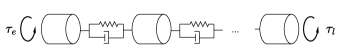
The mechanical driveline of a variable speed industrial drive can be modeled as discrete inertias connected with inertia free elastic elements (see Fig. 2). The complex driveline system can be characterized by two transfer functions that describe the response of the shaft speed to the applied electrical torque and the load torque:
| (9) |
where , and are, respectively, the discrete-Fourier transforms (DFT) the shaft speed, electrical and load torque signals.
Similar to the previous approach, the system frequency response is approximated by the reduced order frequency response around each resonant frequency:
| (10) |
The term is an integrator term that is explicitly taken out. The same assumption holds for .
| (11) |
Furthermore, we may assume to be smooth and constant in the neighborhood of the resonance. So the last expression can be simplified to a constant complex value, denoted by in the sequel. That is,
| (12) |
Splitting the real and imaginary parts lead to
| (13) |
where is the parameter vector defined as
II-A Simulation Results
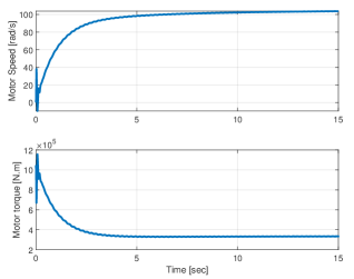
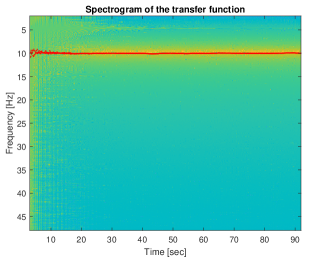
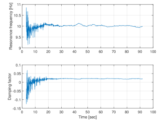
A mechanical driveline is simulated in Matlab/Simulink and the method described above is applied to the driveline signals to estimate a resonant mode. Fig. 3 illustrates the motor speed and torque signals. We use the short-time Fourier transform (STFT) to convert the time-domain signals to the frequency-domain components. Fig. 4 depicts the spectrogram of during the transient and the steady-state. In this simulation, we only look at one resonance. Thus, the RLS algorithm sweeps from Hz to Hz, to detect the resonating frequency, which is initially known to be within this interval. The resulting estimate is plotted in Fig. 4 as red dots, and more clearly in Fig. 5. The actual value of is set to 9.8 Hz. The estimate of the damping factor is also plotted in Fig. 5.
III Summary
A novel solution is proposed for online estimation of the resonant modes. The method, described by a diagram in Fig. 6, is composed of an offline computation, where the data quality and informativity is analyzed[3, 4], followed by an online efficient estimation process based on recursive least square (RLS), providing a computationally efficient solution. The RLS approach is applied to a narrower frequency range only around the resonant frequency, allowing the entire system response to be approximated by a second-order model. This simplification results in less computation for the resonance estimation, which is another novelty of the solution. All of the modules described can be run on an embedded system at a slower sampling rate than the controller or offline.
References
- [1] M. Mercangoez, S. Mastellone, et al., “Damping torsional oscillations at the intersection of variable-speed drives and elastic mechanical systems,” ABB Review Innovation Journal, Tech. Rep., 2016.
- [2] R. Fairbairn, G. Jennings, and R. Harley, “Turbogenerator torsional mechanical modal parameter identification from on-line measurements,” IEEE Transactions on Power Systems, vol. 6, no. 4, pp. 1389–1395, 1991.
- [3] A. Rezaeizadeh, S. Mastellone, F. Bertoldi, and P. A. Hokayem, “Structure and parameters estimation of complex grid impedance,” in 2024 European Control Conference (ECC), 2024, pp. 1991–1996.
- [4] A. Rezaeizadeh, “Set membership identification and control of an iterative process,” in 2019 18th European Control Conference (ECC), 2019, pp. 36–41.