Risk-indifference Pricing of American-style Contingent Claims

Rohini Kumar R. Kumar, Department of Mathematics, Wayne State University, 656 W. Kirby Street, Detroit, MI 48202, USA (e-mail: rohini.kumar@wayne.edu); Corresponding Author.    Frederick “Forrest” Miller F. Miller, Department of Mathematics, Northeastern University, Lake Hall, 360 Huntington Avenue, Boston MA 02115, USA (e-mail: miller.f@northeastern.edu).    Hussein Nasralah H. Nasralah, Department of Mathematics and Statistics, University of Michigan–Dearborn, 4901 Evergreen Road, Dearborn, MI 48128, USA (e-mail: hnasrala@umich.edu).    Stephan Sturm S. Sturm, Department of Mathematical Sciences, Worcester Polytechnic Institute, 100 Institute Road, Worcester MA 06109, USA (e-mail: ssturm@wpi.edu).
Abstract

This paper studies the pricing of contingent claims of American style, using indifference pricing by fully dynamic convex risk measures. We provide a general definition of risk-indifference prices for buyers and sellers in continuous time, in a setting where buyer and seller have potentially different information, and show that these definitions are consistent with no-arbitrage principles. Specifying to stochastic volatility models, we characterize indifference prices via solutions of Backward Stochastic Differential Equations reflected at Backward Stochastic Differential Equations and show that this characterization provides a basis for the implementation of numerical methods using deep learning.

Keywords: American Options, Fully Dynamic Convex Risk Measures, Indifference Pricing, (Reflected) Backward Stochastic Differential Equations.

Mathematics Subject Classification (2020): 91G20, 91G70, 60H10.

JEL classification: D81, G13, C61.

1 Introduction

The pricing of American style derivatives remains an active area of research. Not only are most single stock options of American style, applications to real options, i.e., the valuation of capital investments using option-pricing methods, abound. The absence of a closed-form benchmark (as the Black–Scholes formula in the European case) makes them a target for research in numerical methods. Additionally, theoretical questions on optimal stopping in nonlinear market models saw recent progress, in particular in incomplete markets.

While the no-arbitrage principle guarantees a unique price in complete markets, in incomplete markets it provides only price bounds (super- and sub-hedging prices) that are typically very wide and do not provide a practical indication of a reasonable price. Therefore, further techniques have been developed to characterize fair and reasonable prices. One of the most prominent ones is indifferences pricing, developed first by Hodges and Neuberger [27]; see the book [9] (edited by Carmona) for a survey. The goal is to establish a threshold or reservation price, at which a potential buyer or seller is indifferent between buying the claim for this price or not buying it, while in either case allowing for continuous trading in the underlying market. Originally developed in a framework of utility maximization, it has been extended to other criteria, such as forward performance measures [38] and risk measures [4, 33]. The formulation via convex dynamic risk measures is in particular attractive, as it is not only nicely connected to the theory of Backward Stochastic Differential Equations (BSDEs), but relies on concepts widely used in the industry and in line with the current regulatory framework [28, Section 12].

Monetary risk measures were first introduced by Artzner, Delbaen, Eber and Heath [2] in the form of coherent measures of risk and then generalized to convex risk measures by Föllmer and Schied [22] and Fritelli and Rosazza Gianin [23]. To capture the time evolution of risk, conditional and dynamic versions have been developed (see, e.g., Cheridito, Delbean and Kupper [10]), and a close connection to Backward Stochastic Differential Equations has been established, see, e.g., Peng [42] and Rosazza Gianin [43]. Most recently fully dynamic convex risk measures became a focus point, i.e., risk measures where both time parameters, the horizon and the evaluation time are considered dynamic, see [8] and [17]. A crucial property in this context is time consistency; it has been studied extensively, see, e.g., the overview papers by Acciaio and Penner [1] and Bielecki, Cialenco and Pitera [7] in discrete time and Rosazza Gianin and DiNunno [17] for fully time-consistent risk measures in continuous time.

The use for indifference pricing was pioneered by Xu [48] and Barrieu and El Karoui [3], generalizing earlier results by Rouge and El Karoui [44] for exponential utility which can be seen as an entropic risk measure en guise and studied systematically in a general setting by Klöppel and Schweizer [33] and Barrieu and El Karoui [4]. Applications to stochastic volatility models and the inverse problem of calibrating risk measures to market data has been studied in Sircar and Sturm [45] and Kumar [36], see also [21].

Indifference pricing for American options appeared first in the study of transaction costs by Davis and Zariphopoulou [15], extending work by Davis, Panas and Zariphpoulou [14] for the European case. The literature encompasses [6, 13, 25, 35, 37, 38, 41, 47, 49, 50] who use utility functions, stochastic differential utilities and forward performance processes as criteria for indifference, we are not aware of any use of dynamic risk measures for the American case (despite the use of Reflected Backward Stochastic Differential Equations for American options dating back to El Karoui, Pardoux and Quenez [20]). For a full discussion of the papers of indifference pricing of American options, we refer to Section 2.5.

The conceptual challenges in implementing indifference pricing stem from the fact that option buyer and seller share different perspectives and the seller’s pricing consideration has to take into account the buyer’s exercise decision. This calls for a careful consideration of which strategies are admissible - something that has been carefully studied in the case of finitely many payoff options by Kühn [35] and whose perspective we amend with a genral counterpart. The pricing by the buyer is slightly more straightforward, however one has to carefully consider at which time one imposes indifference (at the exercise time or maturity?) and how this connects to the notion of arbitrage. In our opinion clarity is best achieved when considering a general case, where one allows buyer and seller to work in different filtrations, reflecting difference in access to market information.

We then specialize to the setting of stochastic volatility models, following the general setup of [45] and [36]. We find that the American indifference prices can be described through Backward Stochastic Differential Equations reflected at Backward Stochastic Differential equations (BSDE-R-BSDEs for short), i.e., Reflected Backward Stochastic Differential Equations (RBSDEs) for which the reflection boundary is given by a BSDE itself. This structure reflects that risk mitigation through trading in the market continues after the exercise of the option – we observe that the reflecting boundary encapsulates, in addition to the exercise value of the option, the risk of holding a zero contract from exercise time to maturity (cf. Remark 3.6). Also, in this setting, the proof of the characterization of the seller’s price requires a substantial amount of work, while the characterization of the buyer’s price is more straightforward. We illustrate our findings by means of a numerical example, the pricing of an American put option, for which we use deep learning methods to simulate the BSDE-R-BSDEs.

New methods on solving BSDEs and RBSDEs through deep learning have been proposed recently and show much promise. Initially, E, Han and Jentzen developed the DEEP BSDE Solver as a forward scheme [18, 26], able to tackle high dimensional problems. A global backward scheme, the Backward Deep BSDE Method was developed by Wang, Chen, Sudjianto, Liu and Shen [46] and studied in detail by Gao, Gao, Hui and Zhu [24], who also analyze the convergence in the case of Lipschitz drivers and show how to use the scheme for Bermudan options. Huré, Pham and Warin [30] introduced schemes based on dynamic programming, namely the Deeep Backward Dynamic Programming schemes, containing in particular one for RBSDEs on which our simulations rely. Recent overview articles on work in this general direction can be found in the papers by E, Jentzen and Han [19] as well as Chessari, Kawai, Shinozaki and Yamada [11].

The paper is structured as follows. Section 2 provides a general setup for the risk-indifference pricing of claims of American style, with minimal conditions on the risk measures involved and considering potentially different information available to buyers and sellers. Section 3 studies the risk-indifference pricing of American claims in stochastic volatility models via BSDE-R-BSDEs, and Section 4 provides a numerical implementation via deep learning. Section 5 concludes by reviewing the contributions of the current work.

2 Risk-indifference pricing

To elucidate the conceptual ideas at the heart of our problem, we initially consider general risk measures and American contingent claims in a general semimartinglae setup, in which the buyer and seller have access to different information represented by different filtrations. We first explain the market setup and the notion of fully dynamic risk measures, before defining the indifference prices from a buyer’s and seller’s perspective and showing that they are free of arbitrage. We conclude this general section by reviewing our methodology against the backdrop of the existing literature on indifference pricing of American claims..

2.1 Setup

We consider a filtered probability space $(\Omega,\mathcal{F},\mathbb{G},\mathbb{P})$ with complete and right-continuous filtration $\mathbb{G}=(\mathcal{G}_{t})_{0\leq t\leq T}$ assuming $\mathcal{G}_{T}=\mathcal{F}$. We consider a financial market consisting of risky assets modeled by a $d$-dimensional $\mathbb{G}$-continuous semimartingale $\hat{S}$ and a riskless asset modeled by a continuous, non-decreasing $\mathbb{G}$-adapted process $B$.

To exclude arbitrage in the sense of no free lunch with vanishing risk (see [16]), we require the existence of a probability measure $\mathbb{Q}$ under which the discounted asset process $S=\hat{S}B^{-1}$ is a local $\mathbb{G}$-martingale. The information of the buyer of the option is given by the complete and right-continuous filtration $\mathbb{F}^{\text{buy}}$, while that of the seller is $\mathbb{F}^{\text{sell}}$; $\mathbb{F}^{S,B}\subseteq\mathbb{F}^{\text{sell}},\mathbb{F}^{\text{buy}}\subseteq\mathbb{G}$, where $\mathbb{F}^{S,B}$ denotes the (augmented) natural filtration generated by risky and riskless assets. For general statements that do not require one particular filtration, we will use the generic $\mathbb{F}$. This setup allows us to model situations where the seller and buyer rely on additional, potentially differential, private information (and randomization), while precluding arbitrage opportunities.

Trading in the market is continuous and self-financing. A portfolio $\hat{V}$ at time $t$ is given by holding $h_{t}$ shares of $\hat{S}$ and $\eta_{t}$ shares of $B$, hence

$$\hat{V}_{t}=h_{t}\hat{S}_{t}+\eta_{t}B_{t}$$

for all $t\in[0,T]$ where $h,\eta\in\mathcal{H}_{\text{buy/sell}}$, the set of $\mathbb{F}^{\text{buy/sell}}$-predictable strategies, for the buyer (resp. seller). For the discounted portfolio dynamics $V=\hat{V}B^{-1}$ we have therefore (starting with zero initial wealth), $V_{t}=\int_{0}^{t}h_{s}\,dS_{s}.$ To mark the dependence of the portfolio on the hedging strategy $h$ we will use a superscript, writing $V^{h}$. To avoid doubling strategies, we will restrict ourselves to strategies with wealth bounded from below. The set of bounded claims hedgeable at no cost from time $t$ onwards is

$$\mathcal{C}^{\text{buy/sell}}_{t.T}:=\biggl{\{}V^{h}_{T}\,:\,V_{\cdot}^{h}=\int_{t}^{\cdot}h_{s}\,dS_{s}\geq c\text{ for some constant }c\in\mathbb{R},h\in\mathcal{H}_{\text{buy/sell}}\biggr{\}}\cap L^{\infty}(\Omega,\mathcal{F},\mathbb{P}).$$

The goal of the paper is to determine a price for an American style contingent claim $\hat{\xi}$, i.e., an almost surely continuous, bounded and $\mathbb{F}^{S,B}$-adapted process that can be exercised by the buyer at an $\mathbb{F}^{\text{buy}}$-stopping time $\tau$, paying $\hat{\xi}_{\tau}$ where $\tau$ is a stopping time either on $[0,T]$ (American style claim) or a closed countable subset of it (Bermudan style claim). We denote the set of all $\mathbb{G}$-stopping times larger than or equal to $t$ by $\mathcal{T}_{t,T}$ and wite $\mathcal{T}_{t,T}^{\text{buy/sell}}$ for the stopping times measurable with respect to the buyer’s (resp. seller’s) filtration. In line with the notation introduced above we write $\xi=\hat{\xi}B^{-1}$ for the discounted claim.

The absence of arbitrage in the financial market consisting of $\hat{S}$ and $B$ guarantees the existence of an arbitrage free price for the derivative $\hat{\xi}$. However, unless if the market is complete (i.e., the local martingale measure $\mathbb{Q}$ is unique), the no-arbitrage principle does not provide a unique price, but rather a (practically often very large) interval of arbitrage free prices.

The current article is concerned with the choice of a reasonable price among the multitude of arbitrage free prices. Our pricing method is based on the principle of indifference, i.e., we determine the price for which the buyer (resp. seller) is indifferent between buying the option for this price (and hedging in the underlying market) or not buying the option at all (but still hedging in the market).

The indifference criterion we will use is that of indifference in risk. For that purpose we introduce the notion of fully dynamic convex risk measures (see [8]):

Definition 2.1.

A family of mappings $\rho_{s,t}:L^{\infty}(\Omega,\mathcal{F}_{t},\mathbb{P})\to L^{\infty}(\Omega,\mathcal{F}_{s},\mathbb{P})$, with times $s,\,t$ satisfying $0\leq s\leq t\leq T$, is called a (strongly) time-consistent fully dynamic convex risk measure if it satisfies the following properties:

  • A)

    Monotonicity: For all $\xi_{1},\,\xi_{2}\in L^{\infty}(\Omega,\mathcal{F}_{t},\mathbb{P})$, $\xi_{1}\geq\xi_{2}$ $\mathbb{P}$-a.s., and for all $s\leq t$,

    $$\rho_{s,t}(\xi_{1})\leq\rho_{s,t}(\xi_{2})\quad\mathbb{P}-a.s.$$
  • B)

    Cash-Invariance: For all $\xi\in L^{\infty}(\Omega,\mathcal{F}_{t},\mathbb{P})$, $m_{s}\in L^{\infty}(\Omega,\mathcal{F}_{s},\mathbb{P})$, and for all $s\leq t$,

    $$\rho_{s,t}(\xi+m_{s})=\rho_{s,t}(\xi)-m_{s}\quad\mathbb{P}-a.s.$$
  • C)

    Convexity: For all $\xi_{1},\,\xi_{2}\in L^{\infty}(\Omega,\mathcal{F}_{t},\mathbb{P})$, $\lambda\in[0,1]$, and for all $s\leq t$,

    $$\rho_{s,t}\bigl{(}\lambda\xi_{1}+(1-\lambda)\xi_{2}\bigr{)}\leq\lambda\rho_{s,t}(\xi_{1})+(1-\lambda)\rho_{s,t}(\xi_{2})\quad\mathbb{P}-a.s.$$
  • D)

    Time-consistency: For all $\xi_{1},\,\xi_{2}\in L^{\infty}(\Omega,\mathcal{F}_{u},\mathbb{P})$ and $s\leq t\leq u$,

    $$\rho_{t,u}\bigl{(}\xi_{1}\bigr{)}=\rho_{t,u}\bigl{(}\xi_{2}\bigr{)}\quad\Longrightarrow\quad\rho_{s,u}\bigl{(}\xi_{1}\bigr{)}=\rho_{s,u}\bigl{(}\xi_{2}\bigr{)}\quad\mathbb{P}-a.s.$$

There is also a stronger form of time consistency,

  • D’)

    Strong time-consistency: For all $\xi\in L^{\infty}(\Omega,\mathcal{F}_{u},\mathbb{P})$ and $s\leq t\leq u$,

    $$\rho_{s,t}\bigl{(}-\rho_{t,u}(\xi)\bigr{)}=\rho_{s,u}(\xi)\quad\mathbb{P}-a.s.$$

    This property clearly implies D), so it is a stronger assumption.

An important additional property that follows from this definition (see [33, Section 3]) is

  • F)

    $\mathcal{F}_{t}$-regularity: For all $\xi_{1},\xi_{2}\in L^{\infty}(\Omega,\mathcal{F}_{t},\mathbb{P})$, $A\in\mathcal{F}_{s}$ and $s\leq t$,

    $$\rho_{s,t}\bigl{(}\xi_{1}{\mathchoice{1\mskip-4.0mu\mathrm{l}}{1\mskip-4.0mu\mathrm{l}}{1\mskip-4.5mu\mathrm{l}}{1\mskip-5.0mu\mathrm{l}}}_{A}+\xi_{2}{\mathchoice{1\mskip-4.0mu\mathrm{l}}{1\mskip-4.0mu\mathrm{l}}{1\mskip-4.5mu\mathrm{l}}{1\mskip-5.0mu\mathrm{l}}}_{A^{c}}\bigr{)}=\rho_{s,t}(\xi_{1}\bigr{)}{\mathchoice{1\mskip-4.0mu\mathrm{l}}{1\mskip-4.0mu\mathrm{l}}{1\mskip-4.5mu\mathrm{l}}{1\mskip-5.0mu\mathrm{l}}}_{A}+\rho_{s,t}(\xi_{2}\bigr{)}{\mathchoice{1\mskip-4.0mu\mathrm{l}}{1\mskip-4.0mu\mathrm{l}}{1\mskip-4.5mu\mathrm{l}}{1\mskip-5.0mu\mathrm{l}}}_{A^{c}}.$$

We note that for a time-consistent fully dynamic convex risk measure $\rho$, the residual risk after partial mitigation is also a time-consistent fully dynamic convex risk measure, see [33, Section 4], and we write, for the buyer’s and seller’s perspective respectively,

$\displaystyle\hat{\rho}_{s,t}(\zeta)$ $\displaystyle:=\operatorname*{essinf}_{C\in\mathcal{C}^{\text{buy}}_{s,t}}\rho_{s,t}(\zeta+C),\quad\zeta\in L^{\infty}(\Omega,\mathcal{F}_{t},\mathbb{P}),$
$\displaystyle\check{\rho}_{s,t}(\zeta)$ $\displaystyle:=\operatorname*{essinf}_{C\in\mathcal{C}^{\text{sell}}_{s,t}}\rho_{s,t}(\zeta+C),\quad\zeta\in L^{\infty}(\Omega,\mathcal{F}_{t},\mathbb{P}),$

for the residual risk from the buyers (resp. sellers) perspective. Specifically, we do not require that the risk measures are normalized and note that even if we assume normalization of $\rho$, i.e., $\rho_{s,t}(0)=0$ for all $0\leq s\leq t\leq T$, this property in general does not carry over to $\hat{\rho}$ and $\check{\rho}$.

2.2 Seller’s Price

We start with the discussion of the seller’s price. This is the more intricate problem as the exercise of the option is done by the buyer, not the seller. Thus, the seller has to take into account any potential exercise action by the buyer. She cannot look at indifference at the time of exercise, as this time is not known to her – it is a stopping time measurable with respect to the filtration $\mathbb{F}^{\text{buy}}$ but might not be measurable with respect to $\mathbb{F}^{\text{sell}}$. Additionally, the seller does not know the exercise time as a random variable, but only its realization along the realized path of assets. Moreover, the hedging strategy should, of course, be predictable in the appropriate filtration ($\mathbb{F}^{\text{sell}}$ enlarged by the realized exercise time) to make it practically implementable. The literature contains several definitions of the seller’s price which, however, fall short of these requirements (we discuss details in Section 2.5). We thus start setting up our definition from scratch:

Let $\mathcal{H}_{\text{sell}}$ be the set of predictable processes with respect to $\mathbb{F}^{\text{sell}}$, the information available to the seller. It represents the trading strategies that the seller can implement over the time interval $[0,T]$ without using the information about the actual exercise. From this set we now construct the set of all strategies that the trader can perform if they take the information of the exercise into account.

Definition 2.2.

Let $\mathcal{I}$ denote the set of possible exercise times of the option, which can either be $[0,T]$ or a closed countable subset of $[0,T]$. We define

$$\mathcal{H}^{\prime}_{\text{sell}}:=\bigl{\{}H:\mathcal{I}\times[0,T]\times\Omega\to\mathbb{R}:\forall t\in\mathcal{I},\,H(t,\cdot,\cdot)\in\mathcal{H}_{\text{sell}}\text{ and }H(t_{1},s,\cdot)=H(t_{2},s,\cdot)\text{ for }s\leq t_{1}\wedge t_{2}\bigr{\}}.$$ (1)

Additionally, if $\mathcal{I}=[0,T]$, then all $H\in\mathcal{H}^{\prime}_{\text{sell}}$ must be right-continuous in the first variable, i.e.,

$$\lim_{u\downarrow t}H(u,\cdot,\cdot)=H(t,\cdot,\cdot).$$

Given any choice of strategy, $H\in\mathcal{H}^{\prime}_{\text{sell}}$, we will denote by $h^{\tau}$ the strategy followed when $\tau\in\mathcal{T}_{0,T}$ is the exercise time, in other words,

$$h^{\tau}_{t}(\omega):=H\bigl{(}\tau(\omega),t,\omega\bigr{)}\quad\text{ for }0\leq t\leq T,\,\omega\in\Omega.$$

Observe that, by definition, the strategies in $\mathcal{H}^{\prime}_{\text{sell}}$ have the following “non-anticipativity” property. For any $H\in\mathcal{H}^{\prime}_{\text{sell}}$ and $\tau_{1},\tau_{2}\in\mathcal{T}_{0,T}$,

$$H\bigl{(}\tau_{1}(\omega),s,\omega\bigr{)}=H\bigl{(}\tau_{2}(\omega),s,\omega\bigr{)},\text{ for }s\,\leq\,\tau_{1}(\omega)\wedge\tau_{2}(\omega).$$

As a consequence, we get

$$h^{\tau}_{t}(\omega)=H\bigl{(}\tau(\omega),t,\omega\bigr{)}=H(T,t,\omega){\mathchoice{1\mskip-4.0mu\mathrm{l}}{1\mskip-4.0mu\mathrm{l}}{1\mskip-4.5mu\mathrm{l}}{1\mskip-5.0mu\mathrm{l}}}_{\{\tau(\omega)\geq t\}}+H\bigl{(}\tau(\omega)\wedge t,t,\omega\bigr{)}{\mathchoice{1\mskip-4.0mu\mathrm{l}}{1\mskip-4.0mu\mathrm{l}}{1\mskip-4.5mu\mathrm{l}}{1\mskip-5.0mu\mathrm{l}}}_{\{\tau(\omega)<t\}},$$ (2)

for any $H\in\mathcal{H}^{\prime}_{\text{sell}}$. This decomposition implies that $h^{\tau}$ is a predictable process with respect to the filtration $\mathbb{F}^{\text{sell},\tau}$, $\mathcal{F}^{\text{sell},\tau}_{t}=\bigcap_{\varepsilon>0}\mathcal{K}_{t+\varepsilon}$, $\mathcal{K}_{t}=\mathcal{F}^{\text{sell}}_{t}\vee\sigma(\tau\wedge t)$, see [40, Section 9].

Proposition 2.3.

The process $h^{\tau}$ is $\mathbb{F}^{\text{sell},\tau}$-predictable.

Proof.

By definition, $H(T,\cdot,\cdot)$ is $\mathbb{F}^{\text{sell}}$-predictable, and using (2) we can write

$$h^{\tau}_{t}(\omega)=H(T,t,\omega)+\Bigl{(}H\bigl{(}\tau(\omega),t,\omega\bigr{)}-H(T,t,\omega)\Bigr{)}{\mathchoice{1\mskip-4.0mu\mathrm{l}}{1\mskip-4.0mu\mathrm{l}}{1\mskip-4.5mu\mathrm{l}}{1\mskip-5.0mu\mathrm{l}}}_{\{\tau(\omega)<t\}},$$

so it remains to show that

$$I_{t}:=\Bigl{(}H\bigl{(}\tau(\omega),t,\omega\bigr{)}-H(T,t,\omega)\Bigr{)}{\mathchoice{1\mskip-4.0mu\mathrm{l}}{1\mskip-4.0mu\mathrm{l}}{1\mskip-4.5mu\mathrm{l}}{1\mskip-5.0mu\mathrm{l}}}_{\{\tau(\omega)<t\}}$$

is $\mathbb{F}^{\text{sell},\tau}$-predictable. We prove this by approximating $I_{t}$ by a sequence of $\mathbb{F}^{\text{sell},\tau}$-predictable processes as follows.

Define a sequence of stopping times $\tau_{n}$ by setting $\tau_{n}(\omega)=s_{k}^{n}:=\sup\bigl{\{}s\in\mathcal{I}\,:\,s<(k+1)2^{-n}\wedge T\bigr{\}}$ if $k2^{-n}\leq\tau(\omega)<(k+1)2^{-n}$, for $k=0,\ldots,\lfloor 2^{n}T\rfloor$. Then $\tau_{n}$ are $\mathbb{F}^{\text{buy}}$-stopping times taking finitely many values with $\tau_{n}\downarrow\tau$. Define moreover

$$I^{(n)}_{t}:=\sum_{k=0}^{\lfloor 2^{n}T\rfloor}\tilde{H}\bigl{(}\tau_{n}(\omega),t,\omega\bigr{)}{\mathchoice{1\mskip-4.0mu\mathrm{l}}{1\mskip-4.0mu\mathrm{l}}{1\mskip-4.5mu\mathrm{l}}{1\mskip-5.0mu\mathrm{l}}}_{\{\tau_{n}(\omega)=s_{k}^{n}\}}{\mathchoice{1\mskip-4.0mu\mathrm{l}}{1\mskip-4.0mu\mathrm{l}}{1\mskip-4.5mu\mathrm{l}}{1\mskip-5.0mu\mathrm{l}}}_{\{\tau_{n}(\omega)<t\}},$$

where $\tilde{H}\bigl{(}\tau_{n}(\omega),t,\omega\bigr{)}=H\bigl{(}\tau_{n}(\omega),t,\omega\bigr{)}-H(T,t,\omega)$ and observe that $I^{(n)}_{t}$ is a sum of $\mathbb{F}^{\text{sell},\tau}$-predictable processes: By definition of $H\in\mathcal{H}^{\prime}_{\text{sell}}$, $\tilde{H}\bigl{(}s_{k}^{n},t,\omega\bigr{)}$ is an $\mathbb{F}^{\text{sell}}$-predictable process (and hence $\mathbb{F}^{\text{sell},\tau}$-predictable) for each $k$. Moreover, for each $k$,

$${\mathchoice{1\mskip-4.0mu\mathrm{l}}{1\mskip-4.0mu\mathrm{l}}{1\mskip-4.5mu\mathrm{l}}{1\mskip-5.0mu\mathrm{l}}}_{\{\tau_{n}(\omega)=s_{k}^{n}\}}{\mathchoice{1\mskip-4.0mu\mathrm{l}}{1\mskip-4.0mu\mathrm{l}}{1\mskip-4.5mu\mathrm{l}}{1\mskip-5.0mu\mathrm{l}}}_{\{\tau_{n}(\omega)<t\}}={\mathchoice{1\mskip-4.0mu\mathrm{l}}{1\mskip-4.0mu\mathrm{l}}{1\mskip-4.5mu\mathrm{l}}{1\mskip-5.0mu\mathrm{l}}}_{A^{(n)}_{k}}(t,\omega),$$

where $A^{(n)}_{k}:=(s_{k}^{n},T]\times\{\tau_{n}=s_{k}^{n}\}\subset[0,T]\times\Omega$ is a set in the predictable $\sigma$-algebra $\mathcal{P}(\mathbb{F}^{\text{sell},\tau})$ with respect to the filtration $\mathbb{F}^{\text{sell},\tau}$, as $\bigl{\{}\tau_{n}=s_{k}^{n}\bigr{\}}=\bigl{\{}k2^{-n}\leq\tau(\omega)\wedge s_{k}^{n}<s_{k}^{n}\bigr{\}}$ is $\sigma(\tau\wedge s_{k}^{n})$ measurable and hence $\mathbb{F}^{\text{sell},\tau}_{s_{k}^{n}}$ measurable.

For each $(t,\omega)\in[0,T]\times\Omega$,

$\displaystyle\phantom{==}I_{t}(\omega)-I^{(n)}_{t}(\omega)=\sum_{k=0}^{\lfloor 2^{n}T\rfloor}\Bigl{[}\tilde{H}\bigl{(}\tau(\omega),t,\omega\bigr{)}{\mathchoice{1\mskip-4.0mu\mathrm{l}}{1\mskip-4.0mu\mathrm{l}}{1\mskip-4.5mu\mathrm{l}}{1\mskip-5.0mu\mathrm{l}}}_{\{\tau(\omega)<t\}}-\tilde{H}\bigl{(}\tau_{n}(\omega),t,\omega\bigr{)}{\mathchoice{1\mskip-4.0mu\mathrm{l}}{1\mskip-4.0mu\mathrm{l}}{1\mskip-4.5mu\mathrm{l}}{1\mskip-5.0mu\mathrm{l}}}_{\{\tau_{n}(\omega)<t\}}\Bigr{]}{\mathchoice{1\mskip-4.0mu\mathrm{l}}{1\mskip-4.0mu\mathrm{l}}{1\mskip-4.5mu\mathrm{l}}{1\mskip-5.0mu\mathrm{l}}}_{\{k2^{-n}\leq\tau(\omega)<(k+1)2^{-n}\wedge T\}}$
$\displaystyle=\sum_{k=0}^{\lfloor 2^{n}T\rfloor}\Bigl{[}\tilde{H}\bigl{(}\tau(\omega),t,\omega\bigr{)}\bigl{(}{\mathchoice{1\mskip-4.0mu\mathrm{l}}{1\mskip-4.0mu\mathrm{l}}{1\mskip-4.5mu\mathrm{l}}{1\mskip-5.0mu\mathrm{l}}}_{\{\tau(\omega)<t\leq\tau_{n}(\omega)\}}+{\mathchoice{1\mskip-4.0mu\mathrm{l}}{1\mskip-4.0mu\mathrm{l}}{1\mskip-4.5mu\mathrm{l}}{1\mskip-5.0mu\mathrm{l}}}_{\{\tau_{n}(\omega)<t\}}\bigr{)}-\tilde{H}\bigl{(}\tau_{n}(\omega),t,\omega\bigr{)}{\mathchoice{1\mskip-4.0mu\mathrm{l}}{1\mskip-4.0mu\mathrm{l}}{1\mskip-4.5mu\mathrm{l}}{1\mskip-5.0mu\mathrm{l}}}_{\{\tau_{n}(\omega)<t\}}\Bigr{]}{\mathchoice{1\mskip-4.0mu\mathrm{l}}{1\mskip-4.0mu\mathrm{l}}{1\mskip-4.5mu\mathrm{l}}{1\mskip-5.0mu\mathrm{l}}}_{\{k2^{-n}\leq\tau(\omega)<(k+1)2^{-n}\wedge T\}}$
$\displaystyle=\sum_{k=0}^{\lfloor 2^{n}T\rfloor}\Bigl{(}\tilde{H}\bigl{(}\tau(\omega),t,\omega\bigr{)}-\tilde{H}\bigl{(}\tau_{n}(\omega),t,\omega\bigr{)}\Bigr{)}{\mathchoice{1\mskip-4.0mu\mathrm{l}}{1\mskip-4.0mu\mathrm{l}}{1\mskip-4.5mu\mathrm{l}}{1\mskip-5.0mu\mathrm{l}}}_{\{\tau_{n}(\omega)<t\}}{\mathchoice{1\mskip-4.0mu\mathrm{l}}{1\mskip-4.0mu\mathrm{l}}{1\mskip-4.5mu\mathrm{l}}{1\mskip-5.0mu\mathrm{l}}}_{\{k2^{-n}\leq\tau(\omega)<(k+1)2^{-n}\wedge T\}}+\tilde{H}\bigl{(}\tau(\omega),t,\omega\bigr{)}{\mathchoice{1\mskip-4.0mu\mathrm{l}}{1\mskip-4.0mu\mathrm{l}}{1\mskip-4.5mu\mathrm{l}}{1\mskip-5.0mu\mathrm{l}}}_{\{\tau(\omega)<t\leq\tau_{n}(\omega)\}}.$

Thus, $I_{t}(\omega)$ is the pointwise limit of $I^{(n)}_{t}(\omega)$ for each $(t,\omega)$ as $n\to\infty$, since $\tau_{n}(\omega)\downarrow\tau(\omega)$ and by right-continuity of $s\mapsto H(s,t,\omega)$. ∎

Note that while all process in $\mathcal{H}^{\prime}_{\text{sell}}$ are $\mathbb{F}^{\text{sell},\tau}$-predictable, not all $\mathbb{F}^{\text{sell},\tau}$-predictable processes are contained in $\mathcal{H}^{\prime}_{\text{sell}}$. Specifically, $\mathcal{H}^{\prime}_{\text{sell}}$ contains only the processes that are depending on the realization of the stopping time, not on the random variable itself.

Based on this clarification on the informational structure of the problem, we turn our attention to the seller’s risk-indifference price for an American put. Here, the relevant set of hedging strategies in this case is $\mathcal{H}^{\prime}_{\text{sell}}$ as the seller has no prior knowledge of the exercise time of the put; she can only choose from hedging strategies that get updated after the exercise time is observed, thus $\mathcal{H}^{\prime}_{\text{sell}}$ is the set of strategies that is relevant. For any choice of strategy $H\in\mathcal{H}^{\prime}_{\text{sell}}$, the seller will follow the strategy $H(T,t,\omega)$ until $\tau(\omega)$, and after $\tau(\omega)$, she switches to the strategy $H\bigl{(}\tau(\omega),t,\omega\bigr{)}$ which is $\tau(\omega)$ dependent. We emphasize that this strategy $h_{\cdot}^{\tau}(\omega)$ is only $\tau(\omega)$ dependent and not $\tau$ dependent. This is a necessary distinction as the seller only observes $\tau(\omega)$ and may not glean any further knowledge of $\tau$. Given that strategy, the seller has to minimize the risk by considering the worst case over all stopping times. As she does not have insight into the buyer’s information structure, she cannot optimize over $\mathcal{T}_{t,T}^{\text{buy}}$ but has to stick to the information available to her, i.e., use $\mathcal{T}_{t,T}^{\text{sell}}$.

Thus, for initial wealth $x$ and a time-consistent fully dynamic risk measure $\rho$, the seller’s price $P^{\text{sell}}_{t}$ has to satisfy at time $t$

$$\check{\rho}_{t,T}(x)=\operatorname*{essinf}_{H\in\mathcal{H}^{\prime}_{\text{sell}}}\operatorname*{esssup}_{\tau\in\mathcal{T}_{t,T}^{\text{sell}}}\,\rho_{t,T}\biggl{(}x+\int_{t}^{T}h_{s}^{\tau}\,dS_{s}-\xi_{\tau}+P_{t}^{\text{sell}}\biggr{)}.$$

Solving for $P^{\text{sell}}$ and using cash invariance we get

$$P_{t}^{\text{sell}}=\operatorname*{essinf}_{H\in\mathcal{H}^{\prime}_{\text{sell}}}\operatorname*{esssup}_{\tau\in\mathcal{T}_{t,T}^{\text{sell}}}\,\rho_{t,T}\biggl{(}\int_{t}^{T}h_{s}^{\tau}\,dS_{s}-\xi_{\tau}\biggr{)}-\check{\rho}_{t,T}(0).$$ (S)

2.3 Buyer’s Price

We are now turning our attention to the buyer’s perspective. The buyer of the American claim has the right, but not the obligation to exercise the option at any time before maturity $T$. Therefore, she can decide on the $\mathbb{F}^{\text{buy}}$-stopping time $\tau$, which will provide her with a payout of $\xi_{\tau}$. Once the buyer with initial capital $x$ has bought the option at time $t$ for a price $P^{\text{buy}}_{t}$, she will of course try to reduce the risk of her position – thus determine the exercise time $\tau^{\text{buy}}$ by minimizing the risk through both, determining the optimal exercise time and optimal hedging in the market until maturity of the option contract, i.e.,

$$\operatorname*{essinf}_{\tau\in\mathcal{T}_{t,T}^{\text{buy}}}\hat{\rho}_{t,T}\bigl{(}x+\xi_{\tau}-P^{\text{buy}}_{t}\bigr{)}=\operatorname*{essinf}_{\tau\in\mathcal{T}_{t,T}^{\text{buy}}}\operatorname*{essinf}_{C\in\mathcal{C}_{t,T}^{\text{buy}}}\rho_{t,T}\Bigl{(}x+\xi_{\tau}-P^{\text{buy}}_{t}+C\Bigr{)}.$$

Note that this minimization is independent of $P^{\text{buy}}_{t}$ and $x$ due to the cash-invariance property. We also point out that as the exercise time here is decided by the buyer, the knowledge about the exercise time does not add information, thus the hedging strategies are indeed $\mathbb{F}^{\text{buy}}$-predictable processes $\mathcal{H}_{\text{buy}}$. Cash invariance thus implies the explicit representation

$\displaystyle P_{t}^{\text{buy}}=\hat{\rho}_{t,T}(0)-\operatorname*{essinf}_{\tau\in\mathcal{T}_{t,T}^{\text{buy}}}\hat{\rho}_{t,T}\bigl{(}\xi_{\tau}\bigr{)}.$ (B)
Remark 2.4.

If one considers the risk measures as being that of representative agents, one can understand $P_{t}^{\text{buy}}$ and $P_{t}^{\text{sell}}$ as bid and ask prices and their difference as bid-ask spread. In that case it is natural to assume that $\mathbb{F}^{\text{buy}}=\mathbb{F}^{\text{sell}}$ (e.g., both equal $\mathbb{F}^{\text{S,B}})$, so $\mathcal{H}^{\prime}_{\text{sell}}=\mathcal{H}^{\prime}_{\text{buy}}=:\mathcal{H}^{\prime}$ and $\check{\rho}$ and $\hat{\rho}$ agree. In this case, by choosing $(\tau_{n})$, $\tau_{n}\in\mathcal{T}_{t,T}^{\text{buy}}$, as a sequence of stopping times such that $\hat{\rho}_{t,T}\bigl{(}\xi_{\tau_{n}}\bigr{)}\downarrow\operatorname*{essinf}_{\tau\in\mathcal{T}_{t,T}^{\text{buy}}}\hat{\rho}_{t,T}\bigl{(}\xi_{\tau}\bigr{)}$, we get

$\displaystyle P_{t}^{\text{sell}}-P_{t}^{\text{buy}}$ $\displaystyle=\Biggl{(}\operatorname*{essinf}_{H\in\mathcal{H}^{\prime}}\operatorname*{esssup}_{\tau\in\mathcal{T}_{t,T}}\,\rho_{t,T}\biggl{(}\int_{t}^{T}h_{s}^{\tau}\,dS_{s}-\xi_{\tau}\biggr{)}-\hat{\rho}_{t,T}(0)\Biggr{)}-\Bigl{(}\hat{\rho}_{t,T}(0)-\operatorname*{essinf}_{\tau\in\mathcal{T}_{t,T}^{\text{buy}}}\hat{\rho}_{t,T}\bigl{(}\xi_{\tau}\bigr{)}\Bigr{)}$
$\displaystyle=\lim_{n\to\infty}\Biggl{(}\operatorname*{essinf}_{H\in\mathcal{H}^{\prime}}\operatorname*{esssup}_{\tau\in\mathcal{T}_{t,T}}\,\rho_{t,T}\biggl{(}\int_{t}^{T}h_{s}^{\tau}\,dS_{s}-\xi_{\tau}\biggr{)}-\hat{\rho}_{t,T}(0)\Biggr{)}-\Bigl{(}\hat{\rho}_{t,T}(0)-\hat{\rho}_{t,T}\bigl{(}\xi_{\tau_{n}}\bigr{)}\Bigr{)}$
$\displaystyle\geq\lim_{n\to\infty}\Biggl{(}\operatorname*{essinf}_{H\in\mathcal{H}^{\prime}}\,\rho_{t,T}\biggl{(}\int_{t}^{T}h_{s}^{\tau_{n}}\,dS_{s}-\xi_{\tau_{n}}\biggr{)}+\hat{\rho}_{t,T}\bigl{(}\xi_{\tau_{n}}\bigr{)}-2\hat{\rho}_{t,T}(0)$
$\displaystyle=\lim_{n\to\infty}\hat{\rho}_{t,T}\bigl{(}-\xi_{\tau_{n}}\bigr{)}+\hat{\rho}_{t,T}\bigl{(}\xi_{\tau_{n}}\bigr{)}-2\hat{\rho}_{t,T}(0)=\lim_{n\to\infty}2\Bigl{(}\frac{1}{2}\hat{\rho}_{t,T}\bigl{(}-\xi_{\tau_{n}}\bigr{)}+\frac{1}{2}\hat{\rho}_{t,T}\bigl{(}\xi_{\tau_{n}}\bigr{)}\Bigr{)}-2\hat{\rho}_{t,T}(0)$
$\displaystyle\geq\lim_{n\to\infty}2\hat{\rho}_{t,T}\Bigl{(}\frac{-\xi_{\tau_{n}}+\xi_{\tau_{n}}}{2}\Bigr{)}-2\hat{\rho}_{t,T}(0)=0,$

where the last inequality is by the convexity of the risk measure. This shows that the definition indeed yields a non-negative bid-ask spread.

2.4 Arbitrage

We have to make sure that the notions of seller’s and buyer’s prices introduced above are free of arbitrage, i.e., a buyer/seller can not make an arbitrage by buying/selling the option at the price $P^{\text{buy/sell}}$ and trading in the market. The next definition makes this notion precise.

Definition 2.5.

We define arbitrage from the buyer’s and seller’s perspective respectively.

  • A price $p$ at time $t$ provides a seller’s arbitrage opportunity if there is a hedging strategy $\hat{H}\in\mathcal{H}^{\prime}_{\text{sell}}$ such that for some amount $x<p$ and for all stopping times $\tau\in\mathcal{T}_{t,T}^{\text{sell}}$ we have that

    $$x+\int\limits_{t}^{T}\hat{h}^{\tau}_{s}\,dS_{s}-\xi_{\tau}\geq 0,$$

    i.e., the seller can pocket the profit $p-x>0$ at time $t$ while being exposed to no risk of loss at time $T$.

  • A price $p$ at time $t\in[0,T]$ provides a buyer’s arbitrage opportunity if there exists a hedging strategy $\hat{h}\in\mathcal{H}_{\text{buy}}$ together with an exercise strategy $\tau\in\mathcal{T}^{\text{buy}}_{t,T}$ such that for some amount $x>p$,

    $$-x+\int\limits_{t}^{T}\hat{h}_{s}\,dS_{s}+\xi_{\tau}\geq 0,$$

    i.e., the buyer can pocket the profit $x-p>0$ at time $t$ while being exposed to no risk of loss at time $T$.

Proposition 2.6.

The price defined by (S) is free of seller’s arbitrage and the price defined by (B) is free of buyer’s arbitrage.

Proof.

We first show that $p=P_{t}^{\text{sell}}$ does not allow for seller’s arbitrage opportunities. Suppose by contradiction that there exists a seller’s arbitrage opportunity $\hat{H}$ in the sense of Definition 2.5. Then

$\displaystyle\operatorname*{essinf}\limits_{h\in\mathcal{H}^{\prime}_{\text{sell}}}\,\operatorname*{esssup}\limits_{\tau\in\mathcal{T}_{t,T}^{\text{sell}}}\,\rho_{t,T}\Biggl{(}x+\int\limits_{t}^{T}h_{s}^{\tau}\,dS_{s}-\xi_{\tau}\Biggr{)}$ $\displaystyle=\operatorname*{essinf}\limits_{H\in\mathcal{H}^{\prime}_{\text{sell}}}\,\operatorname*{esssup}\limits_{\tau\in\mathcal{T}_{t,T}^{\text{sell}}}\,\rho_{t,T}\Biggl{(}x+\int\limits_{t}^{T}h_{s}^{\tau}\,dS_{s}+\int\limits_{t}^{T}\hat{h}^{\tau}_{s}\,dS_{s}-\xi_{\tau}\Biggr{)}$
$\displaystyle\leq\operatorname*{essinf}\limits_{H\in\mathcal{H}^{\prime}_{\text{sell}}}\,\operatorname*{esssup}\limits_{\tau\in\mathcal{T}_{t,T}^{\text{sell}}}\,\rho_{t,T}\Biggl{(}\int\limits_{t}^{T}h_{s}^{\tau}\,dS_{s}\Biggr{)}$
$\displaystyle=\operatorname*{essinf}\limits_{h\in\mathcal{H}_{\text{sell}}}\,\rho_{t,T}\Biggl{(}\int\limits_{t}^{T}h_{s}\,dS_{s}\Biggr{)}=\check{\rho}_{t,T}(0).$

whence

$$P_{t}^{\text{sell}}=\operatorname*{essinf}\limits_{H\in\mathcal{H}^{\prime}_{\text{sell}}}\,\operatorname*{esssup}\limits_{\tau\in\mathcal{T}_{t,T}^{\text{sell}}}\,\rho_{t,T}\Biggl{(}\int\limits_{t}^{T}h_{s}^{\tau}\,dS_{s}-\xi_{\tau}\Biggr{)}-\check{\rho}_{t,T}(0)\leq x,$$

which contradicts the assumption that $x<P_{t}^{\text{sell}}$ and therefore disproves the existence of a seller’s arbitrage opportunity.

Similarly, assume a buyer’s arbitrage opportunity $(\hat{h},\hat{\tau})$ exists in the sense of Definition 2.5. Employing a similar argument as above, we find

$$\hat{\rho}_{t,T}(x)\geq\hat{\rho}_{t,T}\Biggl{(}\int_{t}^{T}\hat{h}_{s}\,dS_{s}+\xi_{\hat{\tau}}\Biggr{)}=\hat{\rho}_{t,T}\bigl{(}\xi_{\hat{\tau}}\bigr{)}\geq\operatorname*{essinf}\limits_{\tau\in\mathcal{T}_{t,T}^{\text{buy}}}\hat{\rho}_{t,T}\bigl{(}\xi_{\tau}\bigr{)}.$$

Thus, cash invariance implies

$$P_{t}^{\text{buy}}=\hat{\rho}_{t,T}(0)-\operatorname*{essinf}\limits_{\tau\in\mathcal{T}_{t,T}^{\text{buy}}}\hat{\rho}_{t,T}\bigl{(}\xi_{\tau}\bigr{)}\geq x.$$

We therefore conclude $x\leq P_{t}^{\text{buy}}$, contradicting the original assumption that $x>P_{t}^{\text{buy}}$ and thereby disproving the existence of a buyer’s arbitrage. ∎

Note that in the case the buyer’s and seller’s filtration agree, Remark 2.4 also implies that the price (S) is free of buyer’s arbitrage and (B) of seller’s arbitrage. In the case the filtrations differ, no such argument can be made as the strategies live in different domains.

2.5 Comparison with the Existing Literature

The literature on indifference pricing of American options is long. Based on early results on European options in [14], Davis and Zariphopolou [15] explore utility indifference pricing in the presence of transaction costs, studying the singular control problem. This line of research has been deepened by Damgaard [13] and Zakamouline [50] who investigate the problem numerically for hyperbolic resp. constant absolute risk aversion, the latter adding the study of the seller’s price. While all these papers assume asset prices given by geometric Brownian motion, Cosso, Marazzina and Sgarra [12] extend the buyer’s side results to stochastic volatility. Oberman and Zariphopoulou, [41] use the indifference pricing methodology to price options on nontraded assets with dynamics correlated to traded assets from a buyer’s perspective, using exponential utility in a geometric Brownian motion setting. An application to a regime switching model under expected utility indifference from the buyer’s side of view is given by Gyulov and Koleva in [25].

Wu and Dai [47] consider the indifference price of an American claim from a seller’s point of view in a jump diffusion model under exponential utility. Bayraktar and Zhou [6] consider indifference pricing of American options on defaultable claims under exponential utility, for both buyer and seller. And Kühn [35] considers the problem of an option seller with a finite number of choices (such as Bermudan options) for general utility functions.

Two papers extend the problem to time dependent utilities. Leung, Sircar and Zariphopoulou [38] consider forward performance measures and consider the buyer’s indifference price in a stochastic volatility market, contrasting it to previous results for exponential utility in [37]. Yan, Liang and Yang extend the indifference pricing setup in [49] to time dependent, additive stochastic differential utilities and optimal investment and consumption for an investor facing uncertainty about the risk-neutral probability measure. They discuss both seller’s and buyer’s perspectives.

We want to compare in particular the different notions of indifference price used. All papers, even those who consider both buyer’s and seller’s price, work with a single filtration setup. For the buyer’s price, the papers [15, 13, 50, 41, 37, 38, 25] use some form of (backward) stepwise maximization of strategies, after the exercise and before it, which is inspired from the Bellman principle in dynamic programming, solving the Merton problem from the exercise time onwards.

The definition of the buyer’s and seller’s price in [6] compares the expected utility of the hedged payoff for a given price at the time of the exercise with the utility of doing no investment at all. This notion strangely mixes notions of certainty equivalent and indifference price. But even if we adapt this notion in a way to compare buyer’s risk at the time of exercise (determined to be risk-minimizing) and put necessary conditions that a minimal minimizing stopping time exists, this notion is in general not free of arbitrage. For the seller’s price this approach is not even possible, as the potential exercise time is not known to the seller (only to the buyer).

For the seller’s price the precise conditions on the admissibility of strategies are rarely fleshed out and most papers are cavalier about it. Zakamouline [50] uses an analogous version to the buyer’s formulation, but assumes that the seller knows the optimal strategy of the buyer. Kühn [35] alone gives a careful discussion and a precise definition, albeit only for the discrete case with finitely many payoff options. Our definition is essentially a generalization of this framework to the general case. Note that a similar formulation of nonanticipativity was given in [5] in the context of superhedging under model uncertainty. However, contrary to $\mathcal{H}^{\prime}_{\text{sell}}$ in (1) they consider not only the realization of the stopping times, but the stopping times (as random variables) themselves. As the option seller has only information on the actual exercise of the option, not hypothetical different asset price and exercise scenarios, we insist that the formulation should depend only on the realization of the stopping time, a point that Kühn rightfully highlights in [35, Remark 2.3]. (A further slight difference is that we use $s\leq t_{1}\wedge t_{2}$ instead of $s<t_{1}\wedge t_{2}$ which assures $h^{\tau}$ to be a predictable process with respect to $\mathbb{F}^{\tau,\text{sell}}$.)

Finally, the forward performance formulation in [38] and the stochastic differential utility in [49] are due to their recursive nature independent of the time horizon, avoiding in this way the intricacies of the dependence on the horizon of the indifference.

3 Stochastic Volatility Models & BDSE-R-BSDEs

We now turn our attention to a class of specific models to provide explicit representations of risk-indifference prices, following mainly the setup of [45]. Specifically, we assume that the risk-free asset has a constant interest rate and thus $dB_{t}=rB_{t}\,dt$, $B_{0}=1$. The price of the discounted risky asset is given by

$\displaystyle dS_{t}$ $\displaystyle=\bigl{(}\mu(V_{t})-r\bigr{)}S_{t}\,dt+\sigma(V_{t})S_{t}\,dW_{1,t},\quad S_{0}=s,$
$\displaystyle dV_{t}$ $\displaystyle=m(V_{t})\,dt+a(V_{t})\,dW_{2,t},\quad V_{0}=v,$

with correlated Brownian motions $W_{1}$, $W_{2}$ with constant correlation $\rho$. These models are very popular among practitioners and are usually called stochastic volatility models. We will assume that the SDE for $V$ admits a pathwise unique (weak) solution (e.g., by assuming the Yamada–Watanabe conditions that $m$ is Lipschitz and $\sigma$ Hölder continuous with exponent $\beta\geq\frac{1}{2}$ and of at most linear growth), $\mu(V_{t})$ and $\sigma(V_{t})$ do not explode and $\sigma(V_{t})$ is nonnegative, hitting zero with probability zero and satisfying $\int_{0}^{T}|\mu(V_{t})|\,dt<\infty$, $\int_{0}^{T}\sigma^{2}(V_{t})\,dt<\infty$ a.s. To assure the existence of an equivalent local martingale measure via Girsanov transform, we assume that the Doléans exponential $\mathcal{E}\bigl{(}-\int_{0}^{\cdot}\lambda(V_{s})\,dW_{1,s}\bigr{)}_{t}$ is a uniformly integrable martingale for the Sharpe ratio $\lambda(V_{t})=\frac{\mu(V_{t})-r}{\sigma(V_{t})}$ (e.g., by enforcing the Novikov condition $\mathbb{E}\bigl{[}\exp\bigl{(}\frac{1}{2}\int_{0}^{T}\lambda^{2}(V_{s})\,ds\bigr{)}\bigr{]}<\infty$). Moreover, we assume that both seller and buyer have no further information besides the asset prices, hence $\mathbb{F}=\mathbb{F}^{\text{buy}}=\mathbb{F}^{\text{sell}}=\mathbb{F}^{S,B}$. So, the (discounted) American claim $\xi$ is given by an almost surely continuous, bounded and $\mathbb{F}$-adapted process.

We consider risk measures specified via solutions of backward stochastic differential equations (BSDEs). It is well-known (e.g., [4]) that if $g:\Omega\times[0,T]\times\mathbb{R}^{2}\to\mathbb{R}$ is a function satisfying certain properties (e.g., convexity on $\mathbb{R}^{2}$), then $g$ (called a driver) gives rise to a fully dynamic, strongly time-consistent monetary convex risk measure as the first component of the solution $(R,Z_{1},Z_{2})$ to the BSDE given by

$$R_{t}=-\zeta-\int_{t}^{u}g(s,Z_{1,s},Z_{2,s})\,dt-\int_{t}^{u}Z_{1,s}\,dW_{1,s}-\int_{t}^{u}Z_{2,s}dW_{2,t}.$$

I.e., the time $t$ risk of a $\mathcal{F}_{u}$ measurable claim $\zeta$ at time horizon $u$ is given by $\rho_{t,u}(\zeta):=R_{t}$. For our purpose, we will assume that $g$ is just a function of $Z_{1},Z_{2}$. What we are mostly interested in is not the risk itself, but the residual risk when we use hedging in the market to (partially) mitigate risk. For this purpose, we have to be a bit more restrictive.

Definition 3.1.

A driver $g:\mathbb{R}^{2}\to\mathbb{R}$ is called strictly quadratic with derivatives of (at most) linear growth if it satisfies

  1. 1.

    $g\in C^{2,1}(\mathbb{R}^{2})$;

  2. 2.

    $g_{z_{1}z_{1}}(z_{1},z_{2})>0$ for all $z_{1},z_{2}\in\mathbb{R}$;

  3. 3.

    there exists constants $c_{1},c_{2}>0$ such that

    $$c_{1}\Bigl{(}\frac{z_{1}^{2}}{4c_{1}^{2}}-(1+z_{2}^{2})\Bigr{)}\leq g(z_{1},z_{2})\leq c_{2}(1+z_{1}^{2}+z_{2}^{2});$$
  4. 4.

    there exists a constant $c_{3}>0$ such that $\frac{1}{c_{3}}\bigl{(}|z_{1}|-c_{3}(1+|z_{2}|)\bigr{)}\leq|g_{z_{1}}|\leq c_{3}(1+|z_{1}|+|z_{2}|)$;

  5. 5.

    there exists a constant $c_{4}>0$ such that $|g_{z_{2}}|\leq c_{4}(1+|z_{1}|+|z_{2}|)$.

Note that this notion is (slightly) more restrictive then the concept used in [45], relying only on conditions 1-3. In the American case we need the additional conditions as we rely, in the proof of the following theorem, on a comparison theorem for RBSDES (specifically [34, Proposition 3.2]) that requires them (cf. also [39] for a possible slight generalization). Hedging the risk is related to solving a BSDE with driver $g^{*}(-\lambda,z_{2})+\lambda z_{1}$, where the principal part stems from a partial Fenchel-Legendre transform in the component that represents the tradeable instruments.

Definition 3.2.

The risk-adjusted driver $g^{*}:\mathbb{R}^{2}\to\mathbb{R}$ is defined as the partial Fenchel conjugate of $g(z_{1},z_{2})$ in $z_{1}$, i.e., $g^{*}(\zeta,z_{2}):=\sup\limits_{z_{1}\in\mathbb{R}}\{\zeta z_{1}-g(z_{1},z_{2})\}$.

Proposition 3.3.

If $g$ is a strictly quadratic driver with derivatives of linear growth, then $g^{*}$ is also a strictly quadratic driver with derivatives of linear growth.

Proof.

That a strictly quadratic driver $g$ results in a risk-adjusted driver $g^{*}$ which is also strictly quadratic follows Lemma 2.5 of [45]. It remains to be shown that the risk-adjusted driver $g^{*}$ satisfies conditions 4 and 5 of Definition 3.1 if $g$ does.

Suppose condition 4 holds for $g(z_{1},z_{2})$. Let $g_{z_{1}}^{-1}(z_{1},z_{2})$ denote the partial inverse of $g_{z_{1}}(z_{1},z_{2})$ in $z_{1}$. Through the simple variable change $z_{1}=g_{z_{1}}^{-1}(y,z_{2})$, the inequality $\frac{1}{c_{3}}\bigl{(}|z_{1}|-c_{3}(1+|z_{2}|)\bigr{)}\leq|g_{z_{1}}|$ implies $|g_{z_{1}}^{-1}|\leq c_{3}(1+|z_{1}|+|z_{2}|)$, while the inequality $|g_{z_{1}}|\leq c_{3}(1+|z_{1}|+|z_{2}|)$ implies $\frac{1}{c_{3}}(|z_{1}|-c_{3}(1+|z_{2}|))\leq|g_{z_{1}}^{-1}|$, giving

$$\frac{1}{c_{3}}(|z_{1}|-c_{3}(1+|z_{2}|))\leq|g_{z_{1}}^{-1}|\leq c_{3}(1+|z_{1}|+|z_{2}|).$$ (3)

The desired inequality follows by noting $g_{z_{1}}^{-1}=g^{*}_{z_{1}}$.

Next we suppose conditions 4 and 5 both hold for $g(z_{1},z_{2})$. Employing the same variable change as in the argument involving condition 4 above, it follows from condition 5 that $|g_{z_{2}}(g_{z_{1}}^{-1}(z_{1},z_{2}),z_{2})|\leq c_{4}(1+|g_{z_{1}}^{-1}(z_{1},z_{2})|+|z_{2}|)$. The result then follows from observing that $g^{*}_{z_{2}}(z_{1},z_{2})=-g_{z_{2}}(g_{z_{1}}^{-1}(z_{1},z_{2}),z_{2})$, and noting the upper bound obtained on $g^{*}_{z_{1}}=g_{z_{1}}^{-1}$ in (3). ∎

Before proving the main theorem, we want to recall a property of risk measures defined by Brownian BSDEs.

Lemma 3.4.

In the BSDE setting, the strong time-consistency property holds for intermediate stopping times. Specifically, for all $\xi\in L^{\infty}(\Omega,\mathcal{F}_{u},\mathbb{P})$, $s\leq u$, and $\tau\in[s,u]$ an $\mathbb{F}$-stopping time,

$$\rho_{s,\tau}\bigl{(}-\rho_{\tau,u}(\xi)\bigr{)}=\rho_{s,u}(\xi).$$
Proof.

This follows from [4, Theorem 3.21]. ∎

Theorem 3.5.

For any $t\in[0,T]$, the seller’s indifference price (S) can be represented as

$$P_{t}^{\text{sell}}=\check{R}^{\xi}_{t}-\check{R}^{0}_{t},$$

where $(\check{R}^{\zeta},\check{Z}_{1},\check{Z}_{2},\check{K},Y,\bar{Z}_{1},\bar{Z}_{2})$ is the unique solution to the BSDE-reflected BSDE (BSDE-R-BSDE) system

$\displaystyle\left\{\begin{array}[]{ll}\check{R}^{\zeta}_{u}&=\zeta_{T}-\int_{u}^{T}\bigl{(}g^{*}(-\lambda_{s},\check{Z}_{2,s})+\lambda_{s}\check{Z}_{1,s}\bigr{)}\,ds+\check{K}_{T}-\check{K}_{u}-\int_{u}^{T}\check{Z}_{1,s}\,dW_{1,s}-\int_{u}^{T}\check{Z}_{2,s}\,dW_{1,s},\\ Y_{u}&=0-\int_{u}^{T}\bigl{(}g^{*}(-\lambda_{s},\bar{Z}_{2,s})+\lambda_{s}\bar{Z}_{1,s}\bigr{)}\,ds-\int_{u}^{T}\bar{Z}_{1,s}\,dW_{1,s}-\int_{u}^{T}\bar{Z}_{2,s}\,dW_{2,s}\\ \check{R}_{u}&\geq\zeta_{u}+Y_{u}\quad\text{with}\quad\int_{t}^{T}\bigl{(}\check{R}_{s}-(\zeta_{s}+Y_{s})\bigr{)}\,d\hat{K}_{s}=0,\qquad\text{ for }t\leq u\leq T,\end{array}\right.$

with $\zeta=\xi$ resp. $\zeta=0$.

Proof.

Fix $t\in[0,T]$. The goal is to derive an RBSDE expression for

$$\operatorname*{essinf}_{H\in\mathcal{H}^{\prime}}\operatorname*{esssup}_{\tau\in\mathcal{T}_{t,T}}\,\rho_{t,T}\biggl{(}\int_{t}^{T}h_{s}^{\tau}\,dS_{s}-\zeta_{\tau}\biggr{)}$$

for an almost surely continuous, bounded and $\mathbb{F}$-adapted process $\zeta$ for which we can then substitute $\zeta=\xi$ or $\zeta=0$ to get the result. This is done in stages by proving several reformulations of the problem.

We start by considering the claim $\zeta$ for a fixed hedging strategy $H\in\mathcal{H}^{\prime}$ (suppressing the $\omega$-dependence of $H$ in the notation). Using the strong time-consistency of Lemma 3.4 and cash-invariance properties of risk measures, we can express the hedged risk of the American payoff $\zeta$ at stopping time $\tau\in\mathcal{T}_{t,T}$ as

$$\rho_{t,T}\Bigl{(}\int_{t}^{T}h_{s}^{\tau}\,dS_{s}-\zeta_{\tau}\Bigr{)}=\rho_{t,\tau}\biggl{(}\int_{t}^{\tau}H(T,s)\,dS_{s}-\zeta_{\tau}-\rho_{\tau,T}\Bigl{(}\int_{\tau}^{T}H(\tau,s)\,dS_{s}\Bigr{)}\biggr{)}\\ =\rho_{t,\tau}\bigl{(}-U_{\tau}^{t,H}\bigr{)},$$

where

$$U_{u}^{t,H}:=\zeta_{u}-\int_{t}^{u}H(T,s)\,dS_{s}+\rho_{u,T}\Bigl{(}\int_{u}^{T}H(u,s)\,dS_{s}\Bigr{)}$$

for $u\in[t,T]$. Denote the supremum over all stopping times by

$$R^{t,H}_{t}:=\operatorname*{esssup}_{\tau\in\mathcal{T}_{t,T}}\rho_{t,\tau}\bigl{(}-U_{\tau}^{t,H}\bigr{)}.$$

By [34, Proposition 3.1] we can represent $R^{t,H}_{u}=\operatorname*{esssup}_{\tau\in\mathcal{T}_{u,T}}\rho_{t,\tau}\bigl{(}-U_{\tau}^{t,H}\bigr{)}$, for $t\leq u\leq T$, as the first component of the (unique) solution of the RBSDE

$$\left\{\begin{array}[]{ll}&R^{t,H}_{u}=U_{T}^{t,H}+\int_{u}^{T}g\bigl{(}Z_{1,s}^{t,H},Z_{2,s}^{t,H}\bigr{)}\,ds+K_{T}^{t,H}-K_{u}^{t,H}-\int_{u}^{T}Z^{t,H}_{1,s}\,dW_{1,s}-\int_{u}^{T}Z_{2,s}^{t,H}\,dW_{2,s},\\ &R^{t,H}_{u}\geq U_{u}^{t,H},\quad\int_{t}^{T}\bigl{(}R^{t,H}_{r}-U_{r}^{t,H}\bigr{)}\,dK_{r}^{t,H}=0,\quad t\leq u\leq T.\end{array}\right.$$

Next, we have to consider $\operatorname*{essinf}_{H\in\mathcal{H}^{\prime}}R^{t,H}_{t}$. To do so, we first develop an alternative representation for the maximal risk. Define

$$\ddot{R}^{H}_{u}:=R^{t,H}_{u}+\int_{t}^{u}H(T,s)\,dS_{s},$$

and note that it is the first component of the unique solution $\bigl{(}\ddot{R}^{H}_{u},\ddot{Z}_{s}^{H,1},\ddot{Z}_{s}^{H,2},\ddot{K}_{u}^{H}\bigr{)}$ to the RBSDE

$$\left\{\begin{array}[]{ll}\ddot{R}^{H}_{u}&=\zeta_{T}-\int_{u}^{T}H(T,s)\,dS_{s}+\int_{u}^{T}g\bigl{(}\ddot{Z}_{1,s}^{H},\ddot{Z}_{2,s}^{H}\bigr{)}\,ds+\ddot{K}_{T}^{H}-\ddot{K}_{u}^{H}-\int_{u}^{T}\ddot{Z}^{H}_{1,s}\,dW_{1,s}-\int_{u}^{T}\ddot{Z}_{2,s}^{H}\,dW_{2,s},\\ \ddot{R}^{H}_{u}&\geq\ddot{U}_{u}^{H},\quad\int_{t}^{T}\bigl{(}\ddot{R}^{H}_{r}-\ddot{U}_{r}^{H}\bigr{)}\,d\ddot{K}_{r}^{H}=0,\qquad\text{ for }t\leq u\leq T,\end{array}\right.$$

where

$$\ddot{U}_{u}^{H}:=U_{u}^{t,H}+\int_{t}^{u}H(T,s)\,dS_{s}=\zeta_{u}+\rho_{u,T}\Bigl{(}\int_{u}^{T}H(u,s)\,dS_{s}\Bigr{)}$$

for $u\in[0,T]$. Observe that at time $u=t$, $\ddot{R}^{H}_{t}=R^{t,H}_{t}$, and so we proceed to find a BSDE expression for $\operatorname*{essinf}_{H\in\mathcal{H}^{\prime}}\ddot{R}^{H}_{t}$.

The reason for this alternative representation for the maximal risk, $\ddot{R}^{H}$, instead of $R^{t,H}$, now becomes clear: for each $H\in\mathcal{H}^{\prime}$, the BSDE dynamics for $\ddot{R}^{H}$ depends only on the strategy $H(T,\cdot)$ and its reflection barrier $\ddot{U}_{u}^{H}$ depends only on $H(u,\cdot)$, $u\in[t,T)$. We can exploit this to separate the infima as follows:

$$\operatorname*{essinf}_{H\in\mathcal{H}^{\prime}}\ddot{R}^{H}_{u}=\operatorname*{essinf}_{H(T,\cdot)\in\mathcal{H}}\operatorname*{essinf}_{\nu\in\mathcal{H}^{H(T,\cdot)}}\ddot{R}^{\nu}_{u},$$ (4)

(while maintaining the right-continuity property of $H\in\mathcal{H}^{\prime}$ in the first variable), where $\mathcal{H}^{H(T,\cdot)}:=\{\nu\in\mathcal{H}^{\prime}:\nu(T,\cdot)=H(T,\cdot)\}$.

We first find an RBSDE representation for $\tilde{R}_{u}^{H}:=\operatorname*{essinf}_{\nu\in\mathcal{H}^{H(T,\cdot)}}\ddot{R}^{\nu}_{u}$. To this end, let us define for $u\in[t,T)$,

$$\bar{\zeta}_{u}:=\operatorname*{essinf}_{\nu\in\mathcal{H}^{H(T,\cdot)}}\ddot{U}_{u}^{\nu}=\operatorname*{essinf}_{\nu(u,\cdot)\in\mathcal{H}}\ddot{U}_{u}^{\nu}=\zeta_{u}+\check{\rho}_{u,T}(0)$$ (5)

and let $Y_{s}:=\check{\rho}_{s,T}(0)$. Then from [45, Proposition 2.7], we have that $(Y,Z_{1},Z_{2})$ is the unique solution to the BSDE with terminal condition $\zeta_{u}$ and driver

$$\inf_{\nu\in\mathbb{R}}\Bigl{(}-\nu\bigl{(}\mu(V_{t})-r\bigr{)}+g\bigl{(}z_{1}-\nu\sigma(V_{t}),z_{2}\bigr{)}\Bigr{)}=g^{*}\bigl{(}-\lambda_{t},z_{2}\bigr{)}-z_{1}\lambda_{t},$$

with Sharpe ratio $\lambda_{t}=\frac{\mu(V_{t})-r}{\sigma(V_{t})}$. Thus,

$$Y_{u}=0-\int_{u}^{T}\Bigl{(}g^{*}\bigl{(}-\lambda_{s},\bar{Z}_{2,s}\bigr{)}+\lambda_{s}\bar{Z}_{1,s}\Bigr{)}\,ds-\int_{u}^{T}\bar{Z}_{1,s}\,dW_{1,s}-\int_{u}^{T}\bar{Z}_{2,s}\,dW_{2,s}.$$

Following the arguments of [33, Theorem 7.17] we see that the infimum in (5) is attained and the minimizing strategy is independent of $u$. By the comparison principle for quadratic RBSDEs ([34, Proposition 3.2]), we get that $\tilde{R}^{H}_{u}=\operatorname*{essinf}_{\nu\in\mathcal{H}^{H(T,\cdot)}}\ddot{R}^{\nu}_{u}$ satisfies

$$\left\{\begin{array}[]{ll}\tilde{R}^{H}_{u}&=\zeta_{T}-\int_{u}^{T}H(T,s)\,dS_{s}+\int_{u}^{T}g\bigl{(}\tilde{Z}_{1,s}^{H},\tilde{Z}_{2,s}^{H}\bigr{)}\,ds+\tilde{K}_{t,T}^{H}-\tilde{K}_{u}^{H}-\int_{u}^{T}\tilde{Z}^{H}_{1,s}\,dW_{1,s}-\int_{u}^{T}\tilde{Z}_{2,s}^{H}\,dW_{2,s},\\ \tilde{R}^{H}_{u}&\geq\zeta_{u}+Y_{u},\quad\int_{t}^{T}\bigl{(}\tilde{R}^{H}_{r}-(\zeta_{r}+Y_{r})\bigr{)}\,d\tilde{K}_{r}^{H}=0.\end{array}\right.$$

Finally, we take $\operatorname*{essinf}_{H(T,\cdot)\in\mathcal{H}}\tilde{R}_{u}^{H}$, and, following the arguments of [33, Theorem 7.17], get that

$$\check{R}^{\zeta}_{u}:=\operatorname*{essinf}_{H(T,\cdot)\in\mathcal{H}}\tilde{R}_{u}^{H}=\operatorname*{essinf}_{H\in\mathcal{H}^{\prime}}\ddot{R}_{t}^{H}=\operatorname*{essinf}_{H\in\mathcal{H}^{\prime}}R_{t}^{t,H}=\operatorname*{essinf}_{H\in\mathcal{H}^{\prime}}\operatorname*{esssup}_{\tau\in\mathcal{T}_{t,T}}\,\rho_{t,T}\biggl{(}\int_{t}^{T}h_{s}^{\tau}\,dS_{s}-\zeta_{\tau}\biggr{)}$$

has the representation given in the statement of the theorem. This concludes the proof. ∎

Remark 3.6.

We want to stress that the term $\zeta+Y$, $\zeta_{u}+Y_{u}=\zeta_{u}+\check{\rho}_{u,T}(0)$, appearing as reflection boundary has a clear economic interpretation: One has to adapt the naive exercise boundary $\zeta$ by adding the (hedged) risk of the zero contract. Equivalently, as $\zeta_{u}+\check{\rho}_{u,T}(0)=\check{\rho}_{u,T}\bigl{(}-\zeta_{u}\bigr{)}$, one has to take the risk of the payment at the time of the exercise into account, however allowing risk mitigation through trading until maturity.

Analogously, but much easier, we can derive a RBSDE representation for the buyer’s indifference price.

Theorem 3.7.

The buyer’s indifference price (B) can be represented as

$$P_{t}^{\text{buy}}=\hat{R}^{\xi}_{t}-\hat{R}^{0}_{t}$$

where $(\hat{R}^{\zeta},\hat{Z}_{1},\hat{Z}_{2},\hat{K},Y,\bar{Z}_{1},\bar{Z}_{2})$ is the unique solution to the BSDE-R-BSDE

$$\left\{\begin{array}[]{ll}\hat{R}^{\zeta}_{u}&=Y_{T}+\int_{u}^{T}\bigl{(}g^{*}(-\lambda_{s},-\hat{Z}_{2,s})-\lambda_{s}\hat{Z}_{1,s}\bigr{)}\,ds+\hat{K}_{T}-\hat{K}_{u}-\int_{u}^{T}\hat{Z}_{1,s}\,dW_{1,s}-\int_{u}^{T}\hat{Z}_{2,s}\,dW_{2,s},\\ Y_{u}&=0+\int_{u}^{T}\bigl{(}g^{*}(-\lambda_{s},-\bar{Z}_{2,s})-\lambda_{s}\bar{Z}_{1,s}\bigr{)}\,ds-\int_{u}^{T}\bar{Z}_{1,s}\,dW_{1,s}-\int_{u}^{T}\bar{Z}_{2,s}\,dW_{2,s},\\ \hat{R}^{\zeta}_{u}&\geq\zeta_{u}+Y_{u}\quad\text{with}\quad\int_{t}^{T}\bigl{(}\hat{R}^{\zeta}_{r}-(\zeta_{r}+Y_{r})\bigr{)}\,d\hat{K}_{r}^{H}=0.\end{array}\right.$$

with $\zeta=\xi$ resp. $\zeta=0$.

Proof.

Fix $t\in[0,T]$. We aim for an RBSDE expression for

$$-\operatorname*{essinf}_{\tau\in\mathcal{T}_{t,T}}\operatorname*{essinf}_{C\in\mathcal{C}_{t,T}}\,\rho_{t,T}\bigl{(}C+\zeta_{\tau}\bigr{)}$$

for an almost surely continuous, bounded and $\mathbb{F}$-adapted process $\zeta$ for which we can then substitute $\zeta=\xi$ or $\zeta=0$ to get the result. We note first that $\tilde{Y}^{\zeta_{\tau}}$,

$$\tilde{Y}^{\zeta_{\tau}}_{t}:=-\operatorname*{essinf}_{C\in\mathcal{C}_{t,T}}\,\rho_{t,T}\bigl{(}C+\zeta_{\tau}\bigr{)}=-\hat{\rho}_{t,T}(\zeta_{\tau})=-\hat{\rho}_{t,\tau}\bigl{(}-\hat{\rho}_{\tau,T}(\zeta_{\tau})\bigr{)},$$

(by Lemma 3.4) satisfies the BSDE

$$\tilde{Y}^{\zeta_{\tau}}_{t}=-\hat{\rho}_{\tau,T}(\zeta_{\tau})+\int_{t}^{\tau}\Bigl{(}g^{*}\bigl{(}-\lambda_{s},-\tilde{Z}_{2,s}\bigr{)}-\lambda_{s}\tilde{Z}_{1,s}\Bigr{)}\,ds-\int_{t}^{\tau}\tilde{Z}_{1,s}\,dW_{1,s}-\int_{t}^{\tau}\tilde{Z}_{2,s}\,dW_{2,s}$$

following [45, Proposition 2.7]. Now ([34, Proposition 3.1]) implies that $\hat{R}^{\zeta}$,

$$\hat{R}^{\zeta}_{t}:=-\operatorname*{essinf}_{\tau\in\mathcal{T}_{t,T}}-\tilde{Y}^{\zeta_{\tau}}_{t}=\operatorname*{esssup}_{\tau\in\mathcal{T}_{t,T}}\tilde{Y}^{\zeta_{\tau}}_{t},$$

has with $\bar{\zeta}_{u}:=-\hat{\rho}_{u,T}(\zeta_{u})$ the RBSDE representation

$$\left\{\begin{array}[]{ll}\hat{R}^{\zeta}_{u}&=\bar{\zeta}_{T}+\int_{u}^{T}\bigl{(}g^{*}(-\lambda_{s},-\hat{Z}_{2,s})-\lambda_{s}\hat{Z}_{1,s}\bigr{)}\,ds+\hat{K}_{T}-\hat{K}_{u}-\int_{u}^{T}\hat{Z}_{1,s}\,dW_{1,s}-\int_{u}^{T}\hat{Z}_{2,s}\,dW_{2,s},\\ \hat{R}^{\zeta}_{u}&\geq\bar{\zeta}_{u},\quad\int_{u}^{T}\bigl{(}\hat{R}^{\zeta}_{s}-\bar{\zeta}_{s}\bigr{)}\,d\hat{K}_{s}^{H}=0,\quad\bar{\zeta}_{u}:=-\hat{\rho}_{u,T}(\zeta_{u}).\end{array}\right.$$

Noting now that $\bar{\zeta}_{u}=\zeta_{u}-\hat{\rho}_{u,T}(0)$ and writing down the BSDE representation of $Y:=\tilde{Y}^{0}$ using [45, Proposition 2.7] gives the result. ∎

Remark 3.8.

Note that in the case $\zeta=0$, in both Theorem 3.5 and 3.7 the RBSDE and boundary dynamics agree, thus reducing the equation to a classical (non-reflected) BSDE.

4 Numerical Solution via Deep Learning

Solving the BSDE-R-BSDE systems of Theorems 3.5 and 3.7 is not a straightforward task, as we are encountering a four-dimensional problem with two forward and two backward SDEs, one of the backward ones serving as reflection boundary for the other. We rely on the recent breakthroughs in deep learning methods to solve this problem numerically. We first describe our general approach and then provide explicit solutions to a sample problem. The code for this implementation can be found at https://github.com/stesturm/American-risk-indifference.

4.1 Solving BSDE-R-BSDEs using the RDBDP Method

To solve the BSDE-R-BSDE systems of Theorems 3.5 and 3.7, we rely on the Reflected Deep Backward Dynamic Programming (RDBDP) algorithm developed by Huré, Pham and Warin in [30] (provided with more context and discussed in Huré’s PhD thesis [29] as well as by Kharroubi in [31]). We show here the implementation for the seller’s price (see Theorem 3.5), the one for the buyer’s works analogously.

We divide the interval $[0,T]$ equidistantly by a partition $\pi$ of $N$ intervals, setting $t_{i}=\frac{iT}{N}$ for $i\in\{0,1,\ldots N\}$. For the seller of an American style claim $h(S_{t})$ we solve, backwards iteratively, the system

$\displaystyle\min_{\phi_{0,i},\phi_{1,i},\phi_{2,i}\in\mathcal{N}_{i}}\mathbb{E}\biggl{[}\Bigl{|}\phi_{0,i}(S^{\pi}_{t_{i}},V^{\pi}_{t_{i}})-\Bigl{(}Y^{\pi}_{t_{i+1}}-\bigl{(}g^{*}(-\lambda(V^{\pi}_{t_{i}}),\phi_{2,i}(S^{\pi}_{t_{i}},V^{\pi}_{t_{i}}))+\lambda(V^{\pi}_{t_{i}})\phi_{1,i}(S^{\pi}_{t_{i}},V^{\pi}_{t_{i}})\bigr{)}\,\Delta s$
$\displaystyle\phantom{==========}-\phi_{1,i}(S^{\pi}_{t_{i}},V^{\pi}_{t_{i}})\,\Delta W_{1,i}-\phi_{2,i}(S^{\pi}_{t_{i}},V^{\pi}_{t_{i}})\,\Delta W_{2,i}\Bigr{)}\Bigr{|}^{2}\biggr{]},$
$\displaystyle\min_{\hat{\phi}_{0,i},\hat{\phi}_{1,i},\hat{\phi}_{2,i}\in\hat{\mathcal{N}}_{i}}\mathbb{E}\biggl{[}\Bigl{|}\hat{\phi}_{0,i}(S^{\pi}_{t_{i}},V^{\pi}_{t_{i}})-\max\Bigl{(}\zeta_{t_{i}}+Y^{\pi}_{t_{i}},\hat{R}^{\pi}_{t_{i+1}}-\bigl{(}g^{*}(-\lambda(V^{\pi}_{t_{i}}),\hat{\phi}_{2,i}(S^{\pi}_{t_{i}},V^{\pi}_{t_{i}}))+\lambda(V^{\pi}_{t_{i}})\hat{\phi}_{1,i}(S^{\pi}_{t_{i}},V^{\pi}_{t_{i}})\bigr{)}\,\Delta s$
$\displaystyle\phantom{==========}-\hat{\phi}_{1,i}(S^{\pi}_{t_{i}},V^{\pi}_{t_{i}})\,\Delta W_{1,i}-\hat{\phi}_{2,i}(S^{\pi}_{t_{i}},V^{\pi}_{t_{i}})\,\Delta W_{2,i}\Bigr{)}\Bigr{|}^{2}\biggr{]}$
subject to
$\displaystyle\left\{\begin{array}[]{ll}S^{\pi}_{t_{i+1}}&=\bigl{(}\mu(V^{\pi}_{t_{i}})-r\bigr{)}S^{\pi}_{t_{i}}\Delta t+\sigma(V^{\pi}_{t_{i}})S^{\pi}_{t_{i}}\,\Delta W_{1,i},\quad S^{\pi}_{0}=s,\\ V^{\pi}_{t_{i+1}}&=b(V^{\pi}_{t_{i}})\,\Delta t+a(V^{\pi}_{t_{i}})\,\Delta W_{2,i},\quad V^{\pi}_{0}=v,\\ Y^{\pi}_{t_{i}}&=\phi^{*}_{0,i}(S^{\pi}_{t_{i}},V^{\pi}_{t_{i}}),\quad Y^{\pi}_{T}=0,\\ \hat{R}^{\pi}_{t_{i}}&=\hat{\phi}^{*}_{0,i}(S^{\pi}_{t_{i}},V^{\pi}_{t_{i}}),\quad\hat{R}^{\pi}_{T}=h(S^{\pi}_{T}).\end{array}\right.$

where $\Delta W_{1,i}$, $\Delta W_{2,i}$ are the Brownian increments from time $t_{i}$ to $t_{i+1}$ and $\mathcal{N}$, $\hat{\mathcal{N}}$ are the hypothesis spaces for the deep neural networks for the boundary condition resp. the RBSDE (with one dimension for the solution process and two for the adjoint processes each) and $\phi^{*}_{0,i}$, $\hat{\phi}^{*}_{0,i}$ the stepwise optimizers (at time step $i$) of the first component. Practically, we first calculate the boundary condition for all time steps by calculating the solution of the zero terminal condition BSDE process and then adding it to the payoff at early exercise. Using the same Brownian paths by fixing seeds, we calculate the RBSDE process using the boundary condition previously calculated. In this way, we have to solve only a single BSDE for the boundary, that we can use for the seller’s price of any type of American payoff (cf. Remark 3.8). Specifically, we use a deep neural network with $2$ hidden layers and ReLu activation functions, and use the Adam optimizer (cf. [32]) for stochastic gradient descent. The implementation https://github.com/stesturm/American-risk-indifference is in TensorFlow.

4.2 Numerical Illustration

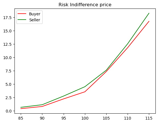
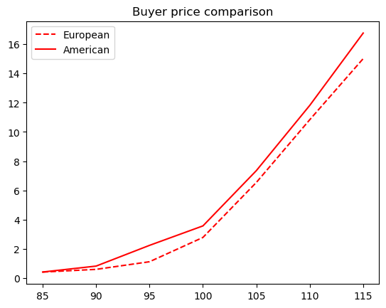
To illustrate the the results, we will consider a specific example along the lines of [45, Section 3] which allows for the direct comparison to the European option example considered there. We assume a classical American put option claim $\hat{\xi}$, thus the discounted claim is $\xi_{t}=\bigl{(}e^{-rt}K-S_{t}\bigr{)}^{+}$, and use distorted entropic risk measures, given by the driver

$$g\bigl{(}z_{1},z_{2}\bigr{)}:=\frac{\gamma}{2}\Bigl{(}z_{1}^{2}+z_{2}^{2}\Bigr{)}+\eta\gamma z_{1}z_{2}+\frac{\eta^{2}\gamma}{2}z_{2}^{2}=\frac{\gamma}{2}\Bigl{(}\bigl{(}z_{1}+\eta z_{2}\bigr{)}^{2}+z_{2}^{2}\Bigr{)}.$$

This driver represents in the case $\eta=0$ a classic entropic risk measure (equivalent to exponential utility) with risk tolerance parameter $\gamma$; the term $\eta$ introduces an additional volatility risk premium. The Fenchel-Legendre transform is given by

$$g^{*}\bigl{(}z_{1},z_{2}\bigr{)}:=\frac{1}{2\gamma}\Bigl{(}z_{1}^{2}-\eta z_{1}z_{2}-\frac{\gamma}{2}z_{2}^{2}\Bigr{)}.$$

As stochastic volatility model we choose the arctangent model

$\displaystyle dS_{t}$ $\displaystyle=\bigl{(}\mu-r\bigr{)}S_{t}\,dt+\sigma(V_{t})S_{t}\,dW_{1,t},\quad S_{0}=s,$
$\displaystyle\sigma(y)$ $\displaystyle=\frac{a}{\pi}\Bigl{(}\arctan(y-1)+\frac{\pi}{2}\Bigr{)}+b,$
$\displaystyle dV_{t}$ $\displaystyle=\alpha\bigl{(}m-V_{t}\bigr{)}\,dt+\nu\sqrt{2\alpha}\Bigl{(}\rho\,dW_{1,t}+\sqrt{1-\rho^{2}}\,dW_{2,t}\Bigr{)},\quad Y_{0}=y.$

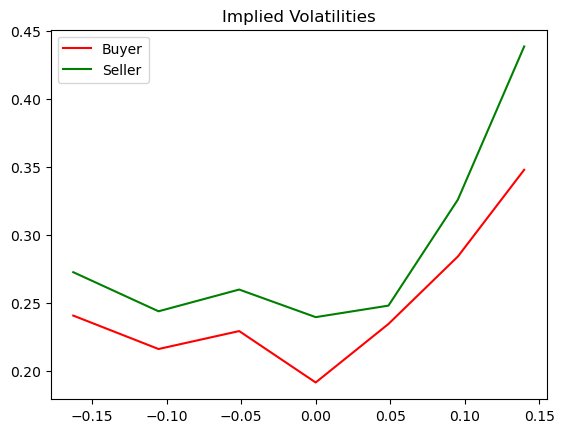
To display the results, we use the market convention to plot in addition to prices (European) implied volatilities by inverting the Black–Scholes formula. We choose as parameters

$\displaystyle r$ $\displaystyle=0.02,\,\mu=0.08,\,a=0.7,\,b=0.03,\,s=100,\,m=0,\,\alpha=5,\,\nu=1,\,\rho=-0.2,\,y=.15,$
$\displaystyle\gamma$ $\displaystyle=1,\,\eta=0.2,\,T=0.25.$

For the hyperparameters of the neural network, we use adaptive epochs, namely 1000 in the beginning and 300 for the last 5 steps, at a batch size of 1100 and a learning rate of 0.01, and we use $N=10$ time steps. We are calculating the prices and the implied volatility for strikes from $K=85$ to $K=115$ in steps of $5$ and plot them against strikes resp. log-moneyness, see Figure 1. We note as comparison that the initial volatility of the stock is $y\approx 15\%$ while the mean-reversion level is $\sigma(m)\approx 20.50\%$.

Refer to caption
Refer to caption
Refer to caption
Figure 1: Left panel: Buyer’s and seller’s prices of American options in terms of strikes. Middle panel: Implied volatility of buyer’s and seller’s prices of American options in terms of log-moneyness. Right panel: Prices of buyer’s prices of European and American options in terms of strikes.

5 Conclusion

Indifference pricing is an important mechanism to establish reasonable reservation prices for buyers and sellers of derivative claims. The current paper explains how this can be done for American-style claims using residual risk after hedging as indifference price mechanism, a choice that is driven by both, the availability of a comprehensive mathematical framework (risk measures and BSDEs) as well as the prevalence of risk measures in industrial practice (as compared to utility-based concepts).

The main contribution of the paper is twofold: On the one hand we provide a general and detailed setup for risk-indifference pricing of American style contingent claims; on the other hand we show how in the case of market incompleteness due to stochastic volatility, the risk-indifference price can be expressed through BSDE-R-BSDEs, backward stochastic differential equations in which the reflection boundary is given itself by a backward stochastic differential equation, reflecting the risk of the position between exercise and maturity. As an add-on, we show how the arising BSDE-R-BSDEs can be solved numerically using deep learning methods and illustrate this on a specific example.

References

  • [1] Beatrice Acciaio and Irina Penner. Dynamic risk measures. In Advanced mathematical methods for finance, pages 1–34. Springer, Heidelberg, 2011.
  • [2] Philippe Artzner, Freddy Delbaen, Jean-Marc Eber, and David Heath. Coherent measures of risk. Math. Finance, 9(3):203–228, 1999.
  • [3] Pauline Barrieu and Nicole El Karoui. Optimal derivatives design under dynamic risk measures. In Mathematics of finance, volume 351 of Contemp. Math., pages 13–25. Amer. Math. Soc., Providence, RI, 2004.
  • [4] Pauline Barrieu and Nicole El Karoui. Pricing, hedging and optimally designing derivatives via minimization of risk measures. In R. Carmona, editor, Indifference Pricing, pages 77–146. Princeton University Press, 2009.
  • [5] Erhan Bayraktar, Yu-Jui Huang, and Zhou Zhou. On hedging American options under model uncertainty. SIAM J. Financial Math., 6(1):425–447, 2015.
  • [6] Erhan Bayraktar and Zhou Zhou. On controller-stopper problems with jumps and their applications to indifference pricing of American options. SIAM J. Financial Math., 5(1):20–49, 2014.
  • [7] Tomasz R. Bielecki, Igor Cialenco, and Marcin Pitera. A survey of time consistency of dynamic risk measures and dynamic performance measures in discrete time: LM-measure perspective. Probab. Uncertain. Quant. Risk, 2:Paper No. 3, 52, 2017.
  • [8] Jocelyne Bion-Nadal and Giulia Di Nunno. Fully-dynamic risk-indifference pricing and no-good-deal bounds. SIAM J. Financial Math., 11(2):620–658, 2020.
  • [9] René Carmona, editor. Indifference pricing. Theory and applications. Princeton Series in Financial Engineering. Princeton University Press, Princeton, NJ, 2009.
  • [10] Patrick Cheridito, Freddy Delbaen, and Michael Kupper. Coherent and convex monetary risk measures for bounded càdlàg processes. Stochastic Process. Appl., 112(1):1–22, 2004.
  • [11] Jared Chessari, Reiichiro Kawai, Yuji Shinozaki, and Toshihiro Yamada. Numerical methods for backward stochastic differential equations: a survey. Probab. Surv., 20:486–567, 2023.
  • [12] Andrea Cosso, Daniele Marazzina, and Carlo Sgarra. American option valuation in a stochastic volatility model with transaction costs. Stochastics, 87(3):518–536, 2015.
  • [13] Anders Damgaard. Computation of reservation prices of options with proportional transaction costs. J. Econom. Dynam. Control, 30(3):415–444, 2006.
  • [14] Mark H. A. Davis, Vassilios G. Panas, and Thaleia Zariphopoulou. European option pricing with transaction costs. SIAM J. Control Optim., 31(2):470–493, 1993.
  • [15] Mark H. A. Davis and Thaleia Zariphopoulou. American options and transaction fees. In Mark H. A. Davis, Darrell Duffie, Wendell H. Fleming, and Steven E. Shreve, editors, Mathematical Finance, pages 47–61. Springer, 1995.
  • [16] Freddy Delbaen and Walter Schachermayer. The mathematics of arbitrage. Springer Finance. Springer-Verlag, Berlin, 2006.
  • [17] Giulia Di Nunno and Emanuela Rosazza Gianin. Fully dynamic risk measures: horizon risk, time-consistency, and relations with BSDEs and BSVIEs. SIAM J. Financial Math., 15(2):399–435, 2024.
  • [18] Weinan E, Jiequn Han, and Arnulf Jentzen. Deep learning-based numerical methods for high-dimensional parabolic partial differential equations and backward stochastic differential equations. Commun. Math. Stat., 5(4):349–380, 2017.
  • [19] Weinan E, Jiequn Han, and Arnulf Jentzen. Algorithms for solving high dimensional PDEs: from nonlinear Monte Carlo to machine learning. Nonlinearity, 35(1):278–310, 2022.
  • [20] N. El Karoui, E. Pardoux, and M. C. Quenez. Reflected backward SDEs and American options. In Numerical methods in finance, volume 13 of Publ. Newton Inst., pages 215–231. Cambridge Univ. Press, Cambridge, 1997.
  • [21] Robert J. Elliott and Tak Kuen Siu. Risk-based indifference pricing under a stochastic volatility model. Commun. Stoch. Anal., 4(1):51–73, 2010.
  • [22] Hans Föllmer and Alexander Schied. Convex measures of risk and trading constraints. Finance Stoch., 6(4):429–447, 2002.
  • [23] Marco Frittelli and Emanuela Rosazza Gianin. Law invariant convex risk measures. In Advances in mathematical economics. Volume 7, volume 7 of Adv. Math. Econ., pages 33–46. Springer, Tokyo, 2005.
  • [24] Chengfan Gao, Siping Gao, Ruimeng Hu, and Zimu Zhu. Convergence of the backward deep BSDE method with applications to optimal stopping problems. SIAM J. Financial Math., 14(4):1290–1303, 2023.
  • [25] Tihomir B. Gyulov and Miglena N. Koleva. Penalty method for indifference pricing of American option in a liquidity switching market. Appl. Numer. Math., 172:525–545, 2022.
  • [26] Jiequn Han, Arnulf Jentzen, and Weinan E. Solving high-dimensional partial differential equations using deep learning. Proc. Natl. Acad. Sci. USA, 115(34):8505–8510, 2018.
  • [27] Stewart D. Hodges and Anthony Neuberger. Optimal replication of contingent claims under transaction costs. Rev. Futures Markets, 8(2):222–239, 1989.
  • [28] John Hull. Risk Management and Financial Institutions. Wiley, United State, 5th edition edition, 2018. includes index.
  • [29] Côme Huré. Numerical Methods and Deep Learning for Stochastic Control Problems and Partial Differential Equations. Theses, Université Paris Diderot (Paris 7), Sorbonne Paris Cité, June 2019.
  • [30] Côme Huré, Huyên Pham, and Xavier Warin. Deep backward schemes for high-dimensional nonlinear PDEs. Math. Comp., 89(324):1547–1579, 2020.
  • [31] Idris Kharroubi. Machine learning approximations for some parabolic partial differential equations. Grad. J. Math., 6(1):1–26, 2021.
  • [32] Diederik P. Kingma and Jimmy Ba. Adam: A method for stochastic optimization. arXiv-preprint 1412.6980, 2017.
  • [33] S. Klöppel and M. Schweizer. Dynamic utility indifference valuation via convex risk measures. NCRR FINRISK working paper No.209. ETH Zürich, 2005. Shorter version published in Math. Finance 17(4):599–627, 2007.
  • [34] M. Kobylanski, J. P. Lepeltier, M. C. Quenez, and S. Torres. Reflected BSDE with superlinear quadratic coefficient. Probab. Math. Statist., 22(1):51–83, 2002.
  • [35] Christoph Kühn. Pricing contingent claims in incomplete markets when the holder can choose among different payoffs. Insurance Math. Econom., 31(2):215–233, 2002.
  • [36] Rohini Kumar. Effect of volatility clustering on indifference pricing of options by convex risk measures. Appl. Math. Finance, 22(1):63–82, 2015.
  • [37] Tim Leung and Ronnie Sircar. Exponential hedging with optimal stopping and application to employee stock option valuation. SIAM J. Control Optim., 48(3):1422–1451, 2009.
  • [38] Tim Leung, Ronnie Sircar, and Thaleia Zariphopoulou. Forward indifference valuation of American options. Stochastics, 84(5-6):741–770, 2012.
  • [39] Marie-Amelie Morlais. Reflected backward stochastic differential equations and a class of non-linear dynamic pricing rule. Stochastics, 85(1):1–26, 2013.
  • [40] Ashkan Nikeghbali. An essay on the general theory of stochastic processes. Probab. Surv., 3:345–412, 2006.
  • [41] A. Oberman and T. Zariphopoulou. Pricing early exercise contracts in incomplete markets. Computational Management Science, 1(1):75–107, 2003.
  • [42] Shige Peng. Nonlinear expectations, nonlinear evaluations and risk measures. In Stochastic methods in finance, volume 1856 of Lecture Notes in Math., pages 165–253. Springer, Berlin, 2004.
  • [43] Emanuela Rosazza Gianin. Risk measures via $g$-expectations. Insurance Math. Econom., 39(1):19–34, 2006.
  • [44] Richard Rouge and Nicole El Karoui. Pricing via utility maximization and entropy. Math. Finance, 10(2):259–276, 2000.
  • [45] Ronnie Sircar and Stephan Sturm. From smile asymptotics to market risk measures. Math. Finance, 25(2):400–425, 2015.
  • [46] Haojie Wang, Han Chen, Agus Sudjianto, Richard Liu, and Qi Shen. Deep learning-based bsde solver for libor market model with application to bermudan swaption pricing and hedging. arXiv-preprint 1807.06622, 2018.
  • [47] Lixin Wu and Min Dai. Pricing jump risk with utility indifference. Quant. Finance, 9(2):177–186, 2009.
  • [48] Mingxin Xu. Risk measure pricing and hedging in incomplete markets. Annals of Finance, 2(1):51–71, January 2006.
  • [49] HuiWen Yan, GeChun Liang, and Zhou Yang. Indifference pricing and hedging in a multiple-priors model with trading constraints. Sci. China Math., 58(4):689–714, 2015.
  • [50] Valeri I. Zakamouline. American option pricing and exercising with transaction costs. J. Comput. Finance, 8(3):81–113, 2005.