SGP-RI: A Real-Time-Trainable and Decentralized IoT Indoor Localization Model Based on Sparse Gaussian Process with Reduced-Dimensional Inputs

Abstract

Internet of Things (IoT) devices are deployed in the filed, there is an enormous amount of untapped potential in local computing on those IoT devices. Harnessing this potential for indoor localization, therefore, becomes an exciting research area. Conventionally, the training and deployment of indoor localization models are based on centralized servers with substantial computational resources. This centralized approach faces several challenges, including the database’s inability to accommodate the dynamic and unpredictable nature of the indoor electromagnetic environment, the model retraining costs, and the susceptibility of centralized servers to security breaches. To mitigate these challenges we aim to amalgamate the offline and online phases of traditional indoor localization methods using a real-time-trainable and decentralized IoT indoor localization model based on Sparse Gaussian Process with Reduced-dimensional Inputs (SGP-RI), where the number and dimension of the input data are reduced through reference point and wireless access point filtering, respectively. The experimental results based on a multi-building and multi-floor static database as well as a single-building and single-floor dynamic database, demonstrate that the proposed SGP-RI model with less than half the training samples as inducing inputs can produce comparable localization performance to the standard Gaussian Process model with the whole training samples. The SGP-RI model enables the decentralization of indoor localization, facilitating its deployment to resource-constrained IoT devices, and thereby could provide enhanced security and privacy, reduced costs, and network dependency. Also, the model’s capability of real-time training makes it possible to quickly adapt to the time-varying indoor electromagnetic environment.

I Introduction

Wi-Fi fingerprinting has emerged as a pivotal technique for indoor localization, leveraging the convenience of existing Wi-Fi infrastructure without the necessity of supplementary hardware. Conventional Wi-Fi fingerprinting consists of an offline phase for the construction of fingerprint databases and the training of a model based on them. This is followed by an online phase for the location estimation of a user or a device using the trained model with newly-measured data at an unknown location [1]. During the offline phase, Wi-Fi fingerprints such as Received Signal Strengths (RSSs), Received Signal Strength Indicators (RSSIs), or Channel State Information are collected to construct databases consisting of training/validation/test datasets, which is quite labor-intensive and time-consuming, spurring an investigation into strategies to alleviate the burdens of constructing fingerprint databases [2, 3]. After the fingerprint database construction a localization algorithm is selected based on the application’s context.

Of many candidates, the advanced machine learning technologies, especially deep learning, have been extensively applied to indoor localization, whose examples are Deep Neural Network (DNN) based methodologies [4], Convolutional Neural Network (CNN) based solutions such as CNNLoc [5], Recurrent Neural Network (RNN) based approaches [6], Transformer based schemes [7], and Graph Neural Network (GNN) based schemes [8] as well as hybrid models combining CNNs with a Transformer architecture [9]. The training of these models requires powerful servers equipped with Graphics Processing Units (GPUs) and considerable amounts of storage space. It is worth noting that despite the reliance on powerful servers, researchers also try to reduce the complexity and training cost of a model by reducing the number of Wireless Access Points (WAPs). For example the latest research used WAP selection network before GNN [8].

After training, these models are employed to furnish indoor localization services, commonly denoted as an online process [1]. Upon a user’s location query, the server utilizes the aforementioned matching algorithms to estimate the user’s most likely location. These algorithms assess the congruence between the user’s newly-measured fingerprint and the stored ones in the database to deduce the location. Subsequently, the system transmits the estimated location data to the user’s device, thereby fulfilling the localization request. This constitutes a fully operational indoor localization service system. As exemplified by the representative models [4, 5, 6, 7, 8, 9], modern indoor localization service systems predominantly rely on intricate centralized models running on servers with high-computational power.

There is a lot of distributed computing power outside centralized servers. At present, the proliferation of network devices has led to a substantial enhancement in both the quantity and computational capabilities of IoT devices, resulting in a notable occurrence of computational redundancy. For instance, numerous WAPs possess a considerable degree of computational power, enabling them to operate Linux-based operating systems such as OpenWrt, which are tailored for routing purposes [10]; these systems are further capable of supporting additional functionalities, such as cloud storage and lightweight server operations, which facilitate traffic-shaping services and the creation of Virtual Private Networks (VPNs). Additionally, devices like the Raspberry Pi serve as a controller for IoT systems, equipped with a comprehensive computational resources, including processors, memory, USB ports, and network interfaces [11]. Therefore, there is a large amount of redundant computational power available on today’s IoT devices. Although it is distributed on different devices and limited in computational power and storage space compared to that of centralized servers, the development of new frameworks and models for indoor localization exploiting the redundant computational power available on distributed IoT devices is an attractive research topic.

Hence, the research objective of this paper is to investigate a decentralized indoor localization framework based on models deployed on IoT devices, which can leverage the redundant computational resources available on IoT devices; the decentralized framework is considered a special case of a distributed one and does not depend on the interaction with other subsystems or the existence of a central server for coordination [12]. By harnessing this untapped computational capacity, an IoT device can offer indoor localization services for a specific area or floor. To enable the decentralized framework, we propose a new real-time-trainable and decentralized IoT indoor localization model based on a Sparse Gaussian Process with Reduced-dimensional Inputs (SGP-RI), where the number and dimension of input data are effectively reduced through Reference Point (RP) and WAP filtering, respectively. Without centralized servers, the decentralized framework enabled by the proposed SGP-RI models, deployed on IoT devices, can provide on-demand indoor localization services even in large-scale multi-building and multi-floor environments.

The major advantages of the decentralized indoor localization based on the SGP-RI models running on IoT devices over the conventional one based on a centralized server can be summarized as follows:

• Reliability: A centralized server under the conventional indoor localization framework is a single point of failure, so its failure could bring down an entire indoor localization system. On the other hand, under the decentralized indoor localization framework, each localization model running on an IoT device handles and stores the localization information of a single floor or part of it, so the impact of one device failure is limited to the corresponding service area.

• Privacy: A centralized server handles location requests from users across all buildings and floors, which could breach the privacy of the users by tracking their locations and/or trajectories. Under the decentralized indoor localization framework, the privacy issue could be limited to a much narrower service area covered by each localization model running on an IoT device.

• Adaptability: Compared to centralized localization models covering the whole service area, a model running on IoT devices is simpler and the corresponding fingerprint database is smaller because they have to cover only a single floor or part of it under the decentralized indoor localization framework, which make it possible to train the model in real time based on the latest data. This enables the model to quickly adapt to the time-varying indoor electromagnetic environment.

The rest of the paper is organized as follows: Section II discusses the challenges in training models on resource-constrained IoT devices. Section III proposes the real-time-trainable IoT indoor localization model based on SGP-RI and the decentralized indoor localization framework based on them, where we discuss the details of Sparse Gaussian Process (SGP) in comparison to standard Gaussian Process (GP), strategies for reducing the numbers of RPs and WAPs, and the generation of inducing inputs for SGP. Section IV details the experimental setup for the indoor localization task and presents the results of the performance evaluation of the proposed model based on SGP-RI in comparison to reference models on both a centralized server and an IoT device. Finally, Section V draws conclusions based on the findings and discussions from the work presented in this paper.

II Challenges in IoT-Based Indoor Localization

A variety of algorithms and techniques have been studied for efficient implementation of indoor localization services based on resource-constrained IoT devices. For example, triangulation using a special implementation of the Angle Of Arrival (AOA) without synchronization was developed for resource-constrained IoT sensors in [13], while efficient solution techniques of trilateration were studied for resource-constrained devices in [12]. Though not specific to indoor localization, in [14] and [15] pre-training methods and new machine learning frameworks were proposed for resource-constrained target platforms, which can be applied to run localization models on IoT devices.

In the case of indoor localization based on Wi-Fi fingerprinting, not only the efficacy of algorithms and models but also the quantity and quality of fingerprint data are critical for localization performance. While data-intensive approaches like Neural Network (NN) models require a substantial amount of training data for higher performance, data-sparse approaches like Bayesian models are capable of being trained with fewer training data for reasonable performance [16]. Given the limited computational resources and storage capacity of resource-constrained IoT devices, therefore, striking the right balance between localization performance and resource utilization, including the amount of data, is of vital importance for IoT-based indoor localization, which makes data-sparse approaches more attractive than data-intensive ones.

As for fingerprint databases, the large numbers of RPs and WAPs in a database do not necessarily guarantee the quality of the database. In [17], it was demonstrated that the spatial distribution of RPs, governed by their inter-spacing and alignment, has a more profound impact on the localization performance than an indiscriminate increase of WAPs and/or RPs. The results suggest that pre-screening of fingerprint databases, which can filter out WAPs and/or RPs not critical for localization, is essential for resource-constrained IoT devices.

The handling of undetected WAPs in Wi-Fi RSSI fingerprint databases is also an important issue. Due to the diverse characteristics of buildings and floors, the number of WAPs detected may vary significantly from one RP to another in large-scale multi-building and multi-floor Wi-Fi fingerprint databases, which results in many gaps in fingerprint databases organized in tabular form like spreadsheets. For instance, the UJIIndoorLoc database [18] indicates the lack of RSSI values from WAPs (i.e., no detection) by using the value of 100; in practice, the values of 100 are replaced by -110 for the continuation of the RSSI values before training a model [4, 19]. The presence of those extrapolated values in databases, however, may adversely affect model performance. GP, for example, imposes strict requirements on the quality and distribution of data. When the dataset is rife with extrapolated values, it may skew the kernel function of GP. Such distortion may bias the model’s interpretation and judgment of the data, potentially resulting in the failure to fit the correct hyperplane. Given the cubic computational complexity of GP, minimizing the number of extrapolated values is particularly crucial when the dataset size is inherently constrained [20]. In general, for non-parametric models including GP, reducing the number of extrapolated values is vital to preserving model performance and efficiency [21]. Though several techniques are proposed to alleviate the difficulties of datasets with gaps (e.g., [22, 23, 24, 25, 26]), most of them are for conventional approaches based on data-intensive NN models running on centralized servers but not for decentralized models based on resource-constrained IoT devices. Consequently, we propose the adoption of the SGP-based model and pre-screening of fingerprint data based on RPs and WAPs as a potential solution to address the aforementioned challenges.

III Real-Time-Trainable Indoor Localization Model Based on SGP

To enable real-time training on resource-constrained IoT devices, we base our indoor localization model on GP regression formulated as a Bayesian linear model, which does not require backpropagation used to train highly-nonlinear NNs. Even without the backpropagation, GP regression still suffers from its cubic scalability with the size of the training dataset. We tackle the issue of poor scalability by approximating GP using SGP with reduced-dimensional inputs (SGP-RI).

III-A From GP to SGP

III-A1 GP

A GP is a stochastic process defined over a continuous domain, which can be denoted as follows [20]:

$$f(\bm{\mathbf{x}})\sim\mathcal{GP}(m(\bm{\mathbf{x}}),k(\bm{\mathbf{x}},\bm{\mathbf{x}}^{\prime})),$$ (1)

where $m(\bm{\mathbf{x}})$ is the mean function and $k(\bm{\mathbf{x}},\bm{\mathbf{x}}^{\prime})$ is the covariance, also called kernel function, evaluated at $\bm{\mathbf{x}}$ and $\bm{\mathbf{x}}^{\prime}$.

Consider a training dataset $\mathcal{D}{=}\{(\bm{\mathbf{x}}_{i},y_{i})\}_{i=1}^{N}$, where $\bm{\mathbf{x}}_{i}$ is a $W$-dimensional column input vector and $y_{i}$ is a scalar output. As we cannot directly observe a function value $f(\bm{\mathbf{x}})$, its observation $y$ can be modeled as follows:

$$y=f(\bm{\mathbf{x}})+\epsilon,$$ (2)

where $\epsilon$ is additive white Gaussian noise with variance $\sigma^{2}$, i.e., $\epsilon{\sim}\mathcal{N}(0,\sigma^{2})$. In Wi-Fi RSSI fingerprinting, $\bm{\mathbf{x}}_{i}$ is a vector of RSSIs from $W$ WAPs measured at the $i$th RP, and $y_{i}$ is one of the coordinates of the $i$th RP, which means that we need two GPs for two-dimensional (2D), single-floor localization. The feature part of the training dataset $\mathcal{D}$ can be represented by an $N{\times}W$ matrix $\bm{\mathbf{X}}{=}[\bm{\mathbf{x}}_{1},\bm{\mathbf{x}}_{2},{\ldots},\bm{\mathbf{x}}_{N}]^{\intercal}$, where each row corresponds to the feature vector of a data point. Likewise, the outputs are collected in an $N$-dimensional column vector $\bm{\mathbf{y}}{=}[y_{1},y_{2},{\ldots},y_{N}]^{\intercal}$.

The predictive distribution of the test outputs $\bm{\mathbf{f}}_{*}$ for test inputs $\bm{\mathbf{X}}_{*}$ is given by

$$p(\bm{\mathbf{f}}_{*}|\bm{\mathbf{X}}_{*},\mathcal{D})=\mathcal{N}(\bm{\mathbf{\mu}}_{*},\bm{\mathbf{\Sigma}}^{2}_{*})$$ (3)

with

$$\bm{\mathbf{\mu}}_{*} =\bm{\mathbf{K}}_{\bm{\mathbf{X}}_{*}\bm{\mathbf{X}}}[\bm{\mathbf{K}}_{\bm{\mathbf{XX}}}+\sigma^{2}\bm{\mathbf{I}}]^{-1}\bm{\mathbf{y}},$$ (4)

$$\bm{\mathbf{\Sigma}}^{2}_{*} =\bm{\mathbf{K}}_{\bm{\mathbf{X}}_{*}\bm{\mathbf{X}}_{*}}-\bm{\mathbf{K}}_{\bm{\mathbf{X}}_{*}\bm{\mathbf{X}}}[\bm{\mathbf{K}}_{\bm{\mathbf{XX}}}+\sigma^{2}\bm{\mathbf{I}}]^{-1}\bm{\mathbf{K}}_{\bm{\mathbf{X}}\bm{\mathbf{X}}_{*}},$$ (5)

where $\bm{\mathbf{K}}_{\bm{\mathbf{XX}}}$, $\bm{\mathbf{K}}_{\bm{\mathbf{X}}\bm{\mathbf{X}}_{*}}$, $\bm{\mathbf{K}}_{\bm{\mathbf{X}}_{*}\bm{\mathbf{X}}}$, and $\bm{\mathbf{K}}_{\bm{\mathbf{X}}_{*}\bm{\mathbf{X}}_{*}}$ are the covariance matrix for the training inputs, the covariance matrix between the training and the test inputs, the covariance matrix between the test and the training inputs, and the covariance matrix for the test inputs, respectively, and $\bm{\mathbf{I}}$ is the identity matrix. (3)–(5) constitute the canonical form of GP regression, and their time complexity is $\mathcal{O}(N^{3})$ with respect to the number of training data $N$, which is dominated by the inversion of $[\bm{\mathbf{K}}_{\bm{\mathbf{XX}}}{+}\sigma^{2}\bm{\mathbf{I}}]$ through Gaussian elimination or Cholesky decomposition [20].

III-A2 SGP

The time complexity of $\mathcal{O}(N^{3})$ makes the application of GP to problems with large datasets impractical. To address the scalability issue, various techniques have been proposed to approximate GP based on SGP, which incorporates a small number $M$ ($M{\ll}N$) of inducing points to reduce the computational complexity of the GP. The primary distinction among SGP models, therefore, lies in the selection of inducing points $\bm{\mathbf{Z}}{=}[\bm{\mathbf{z}}_{1},\bm{\mathbf{z}}_{2},{\ldots},\bm{\mathbf{z}}_{M}]^{\intercal}$ [28].

Once inducing points are selected, we can evaluate the values of $f$ at those inducing points, which are called inducing variables, i.e., $\bm{\mathbf{u}}{=}[u_{1},u_{2},{\ldots},u_{M}]^{\intercal}$, where $u_{i}{=}f(\bm{\mathbf{z}}_{i})$. Variational inference is then employed to construct the approximate posterior distribution based on inducing points and inducing variables, which in turn allows us to derive the approximate posterior distribution of the function values $\bm{\mathbf{f}}_{*}$ at test inputs $\bm{\mathbf{X}}_{*}$.

The posterior distribution of the inducing variables $\bm{\mathbf{u}}$ given the training dataset $\mathcal{D}$ and the inducing points $\bm{\mathbf{Z}}$ is as follows [29]:

$$\begin{multlined}p(\bm{\mathbf{u}}|\mathcal{D},\bm{\mathbf{Z}})=\\ \mathcal{N}(\bm{\mathbf{u}}|\bm{\mathbf{K}}_{\bm{\mathbf{ZZ}}}\bm{\mathbf{Q}}_{\bm{\mathbf{ZZ}}}^{-1}\bm{\mathbf{K}}_{\bm{\mathbf{ZX}}}[\bm{\mathbf{\Lambda}}+\sigma^{2}\bm{\mathbf{I}}]^{-1}\bm{\mathbf{y}},\bm{\mathbf{K}}_{\bm{\mathbf{ZZ}}}\bm{\mathbf{Q}}_{\bm{\mathbf{ZZ}}}^{-1}\bm{\mathbf{K}}_{\bm{\mathbf{ZZ}}}),\end{multlined}p(\bm{\mathbf{u}}|\mathcal{D},\bm{\mathbf{Z}})=\\ \mathcal{N}(\bm{\mathbf{u}}|\bm{\mathbf{K}}_{\bm{\mathbf{ZZ}}}\bm{\mathbf{Q}}_{\bm{\mathbf{ZZ}}}^{-1}\bm{\mathbf{K}}_{\bm{\mathbf{ZX}}}[\bm{\mathbf{\Lambda}}+\sigma^{2}\bm{\mathbf{I}}]^{-1}\bm{\mathbf{y}},\bm{\mathbf{K}}_{\bm{\mathbf{ZZ}}}\bm{\mathbf{Q}}_{\bm{\mathbf{ZZ}}}^{-1}\bm{\mathbf{K}}_{\bm{\mathbf{ZZ}}}),$$ (6)

with

$$\bm{\mathbf{Q}}_{\bm{\mathbf{ZZ}}} =\bm{\mathbf{K}}_{\bm{\mathbf{ZZ}}}+\bm{\mathbf{K}}_{\bm{\mathbf{ZX}}}[\bm{\mathbf{\Lambda}}+\sigma^{2}\bm{\mathbf{I}}]^{-1}\bm{\mathbf{K}}_{\bm{\mathbf{XZ}}},$$ (7)

$$\bm{\mathbf{\Lambda}} =\operatorname*{diag}(\lambda_{1},\ldots,\lambda_{N}),$$ (8)

where

$$\lambda_{i}=[\bm{\mathbf{K}}_{\bm{\mathbf{XX}}}-\bm{\mathbf{K}}_{\bm{\mathbf{XX}}}^{\intercal}\bm{\mathbf{K}}_{\bm{\mathbf{ZZ}}}^{-1}\bm{\mathbf{K}}_{\bm{\mathbf{XX}}}]_{i,i}.$$ (9)

In this case, the predictive distribution of the test outputs $\bm{\mathbf{f}}_{*}$ at test inputs $\bm{\mathbf{X}}_{*}$ given the training dataset $\mathcal{D}$ and the inducing points $\bm{\mathbf{Z}}$, is given by

$$p(\bm{\mathbf{f}}_{*}|\bm{\mathbf{X}}_{*},\mathcal{D},\bm{\mathbf{Z}})=\mathcal{N}(\bm{\mathbf{f}}_{*}|\bm{\mathbf{\tilde{\mu}}}_{*},\bm{\mathbf{\tilde{\Sigma}}}^{2}_{*}),$$ (10)

where

$$\bm{\mathbf{\tilde{\mu}}}_{*} =\bm{\mathbf{K}}_{\bm{\mathbf{X}}_{*}\bm{\mathbf{X}}_{*}}^{\intercal}\bm{\mathbf{Q}}_{\bm{\mathbf{ZZ}}}^{-1}\bm{\mathbf{K}}_{\bm{\mathbf{ZX}}}(\bm{\mathbf{\Lambda}}+\sigma^{2}\bm{\mathbf{I}})\bm{\mathbf{y}},$$ (11)

$$\bm{\mathbf{\tilde{\Sigma}}}^{2}_{*} =\bm{\mathbf{K}}_{\bm{\mathbf{X}}_{*}\bm{\mathbf{X}}_{*}}-\bm{\mathbf{K}}_{\bm{\mathbf{X}}_{*}\bm{\mathbf{X}}_{*}}^{\intercal}(\bm{\mathbf{K}}_{\bm{\mathbf{ZZ}}}^{-1}-\bm{\mathbf{Q}}_{\bm{\mathbf{ZZ}}}^{-1})\bm{\mathbf{K}}_{\bm{\mathbf{X}}_{*}\bm{\mathbf{X}}_{*}}.$$ (12)

The means (i.e., $\bm{\mathbf{\tilde{\mu}}}_{*}$) and the variances (i.e., the diagonal elements of $\bm{\mathbf{\tilde{\Sigma}}}^{2}_{*}$) of the distribution provide the estimates of the test outputs $\bm{\mathbf{f}}_{*}$ and their uncertainties, respectively.

The time complexity of SGP is significantly reduced to $\mathcal{O}(NM^{2})$ compared to $\mathcal{O}(N^{3})$ of GP given $M{\ll}N$ because we can avoid the inversion of the $N{\times}N$ matrix in (4) and (5); the major component is the calculation of $\bm{\mathbf{Q}}_{\bm{\mathbf{ZZ}}}$ in (7) dominated by the matrix multiplication of $\bm{\mathbf{K}}_{\bm{\mathbf{ZX}}}[\bm{\mathbf{\Lambda}}{+}\sigma^{2}\bm{\mathbf{I}}]^{-1}\bm{\mathbf{K}}_{\bm{\mathbf{XZ}}}$, where the complexity of the inversion of the diagonal matrix $[\bm{\mathbf{\Lambda}}{+}\sigma^{2}\bm{\mathbf{I}}]$ is negligible [29].

III-B SGP with Reduced-Dimensional Inputs (SGP-RI)

III-B1 WAP-Based Feature Selection

With SGP based on $M$ inducing variables, we can reduce the computational complexity of the regression to $\mathcal{O}(NM^{2})$. To enable real-time training of and inference with the SGP regression model on resource-constrained IoT devices, we go one step further to reduce the dimensionality of input data (i.e., $W$), which is hardly taken into account in the analysis of computational complexity of GP models in the literature. For example, the complexity of the calculation of the covariance matrix $\bm{\mathbf{K}}_{\bm{\mathbf{ZZ}}}$ in (6) is $\mathcal{O}(M^{2}W)$ because there are $M{\times}M$ elements, each of which depends on two $W$-dimensional vectors. Note that, though the various calculations depending on $W$ are not captured in the computational complexity of SGP regression, they still affect the execution time of a model running on an IoT device.

For dimensionality reduction in indoor localization based on Wi-Fi fingerprinting, we propose a simple, heuristic feature selection scheme to filter out WAPs not providing valuable features for the localization task. First of all, we can filter out WAPs undetectable on a target floor in a large-scale multi-building and multi-floor fingerprint database or WAPs no longer active on a target time slot in a dynamic fingerprint database providing multiple time slices over a long period of time, which are superfluous for the learning process. Then, we can additionally filter out WAPs based on their activities and similarity level, whose details are given in Algorithm 1. Applying Algorithm 1 to the feature matrix $\bm{\mathbf{X}}{\in}\mathbb{R}^{N{\times}W}$, we can reduce its number of columns from $W$ to $V$, where the similarity threshold value in the definition of $\eta$ (i.e., 3) and the comparison threshold of 0.85 for $\eta$ are determined based on the experiments with the two databases discussed in Section IV.

Note that, because the WAP-based feature selection given in Algorithm 1 targets resource-constrained IoT devices, we intentionally limit its complexity during its design. Fig. 1 visually illustrates Algorithm 1 with the RSSIs measured on the Floor 3 of Building 1 of the UJIIndoorLoc database [18] as an example: In this example, the variance of the RSSI vector for WAP223 is found to be greater than that of WAP222. As described in Algorithm 1, we can construct the difference vector $\bm{\mathbf{\Delta}}$ as a vector of element-wise absolute values of the difference between the two RSSI vectors. As shown in Fig. 1, only the RSSI value highlighted by the red circle at the upper right corner is significantly different, so more than $85\%$ of the elements in $\bm{\mathbf{\Delta}}$ are less than 3 (i.e, $\eta{>}0.85$). Next, the index $k$ of the maximum value in $\bm{\mathbf{\Delta}}$ is obtained, and the RSSI values at this index for WAP223 and WAP222 are compared. As indicated by the brighter color of the RSSI sample in the red circle of Fig. 1, the RSSI value of WAP222 is greater, so the column belonging to WAP223 is filtered out.

Data: The feature part $\bm{\mathbf{X}}{\in}\mathbb{R}^{N{\times}W}$ of a training dataset $\mathcal{D}=\left(\bm{\mathbf{X}},\bm{\mathbf{y}}\right)$, where $X_{i,j}$ is the RSSI from $j$th WAP measured at $i$th RP; a target number of columns $V({<}W)$.

Result: A feature part with $V$ columns.

Sort the columns of $\bm{\mathbf{X}}$ based on column-wise variances in a decreasing order;

$c\leftarrow W$;

for $j=1$ to $W{-}1$ do

       $\bm{\mathbf{\Delta}}\leftarrow\big{|}\textnormal{{Column(}}\textnormal{\emph{$\bm{\mathbf{X}},j$}}\textnormal{{)}}-\textnormal{{Column(}}\textnormal{\emph{$\bm{\mathbf{X}},j{+}1$}}\textnormal{{)}}\big{|}$;

        /* element-wise absolute values */

       $\eta\leftarrow\left.\left(\text{\# of elements of $\bm{\mathbf{\Delta}}$ less than or equal to 3}\right)\middle/N\right.$;

       if $\eta=1$ 

             Remove $(j{+}1)$th column from $\bm{\mathbf{X}}$;

             $c\leftarrow c-1$;

            

       else if $\eta\geq 0.85$ 

             $k\leftarrow$ row index of the maximum element of $\bm{\mathbf{\Delta}}$;

             if $X_{k,j}<X_{k,j+1}$ 

                   Remove $j$th column from $\bm{\mathbf{X}}$;

                  

            else

                   Remove $(j{+}1)$th column from $\bm{\mathbf{X}}$;

                  

             end if

            $c\leftarrow c-1$;

            

       end if

      if $c{=}V$ 

             break;

            

       end if

      

end for

Algorithm 1 Feature selection based on WAP RSSI similarity.

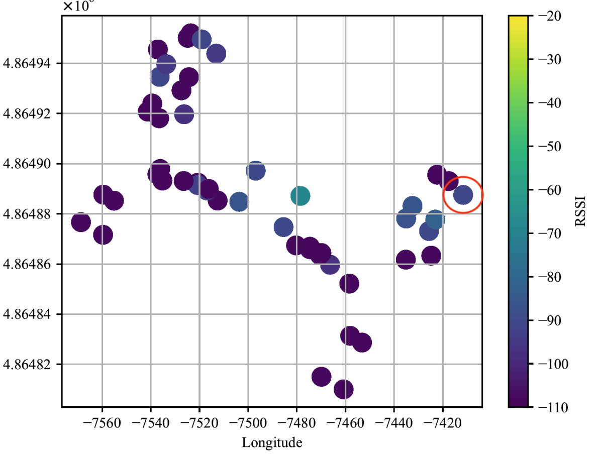
Figure 1: Comparison of RSSIs from (a) WAP222 and (b) WAP223, where the red circle highlights the difference between them.

III-B2 RP-Based Inducing Point Selection

Various SGP algorithms have been proposed for the selection of inducing points, which can be chosen from the original training data or optimized as part of the hyperparameters [28]. For the latter, typically iterative algorithms (e.g, Limited-storage Broyden-Fletcher-Goldfarb-Shanno (L-BFGS) algorithm [30]) are used to maximize an objective function (e.g., marginal likelihood [29]), which is not suitable for resource-constrained IoT devices due to the significant computational overhead. Like the WAP-based feature selection for input dimensionality reduction, we therefore propose a heuristic inducing point selection scheme based on RPs, which is computationally efficient.

Wi-Fi fingerprint databases can be constructed based on diverse RSSI collection methods, i.e., insourcing, crowdsourcing, and their hybrid. In the case of insourcing, participants of a project collect RSSIs at pre-arranged, regularly-spaced (e.g., grid) RPs repeatedly; on the other hand, in the case of crowdsourcing, a large number of volunteers collect RSSIs while moving freely without pre-arranged RPs, resulting in uneven RSSI spatial distributions. As there are multiple RSSIs measured at the same RP (i.e., insourcing) or the RPs located in a small area (i.e., crowdsourcing) whose characteristics are similar to one another, we select only a few of them as inducing inputs.

For computationally-efficient implementation on resource-constrained IoT devices, we divide the covered area into a small rectangular grid and randomly select a certain number of inputs from each grid. The details of the selection of inducing points based on RPs are described in Algorithm 2, where the number of grid cells $L$ and the threshold $\eta$ are design parameters. The algorithm gives the number of inducing points $M{=}|\mathcal{Z}|$, which is less than or equal to $L{\times}\eta$.

Data: A training dataset $\mathcal{\tilde{D}}{=}\{(\bm{\mathbf{x}}_{i},\bm{\mathbf{y}}_{i})\}^{N}_{i=1}$ where $\bm{\mathbf{y}}_{i}$ is the 2D coordinates of the RP for an RSSI vector $\bm{\mathbf{x}}_{i}$; a set of rectangular grid cells $\mathcal{G}{=}\{g_{i}\}^{L}_{i=1}$; a threshold $\eta$ for the maximum number of inputs per grid cell.

Result: A set of inducing points $\mathcal{Z}$.

Initialize subsets $\mathcal{Z}_{l}~{}(l{=}1,{\ldots},L)$ s.t. $x_{i}{\in}\mathcal{Z}_{l}$ if $\bm{\mathbf{y}}_{i}{\in}g_{l}$;

for $l=1$ to $L$ do

      if $|\mathcal{Z}_{l}|{>}\eta$ 

            Remove $|\mathcal{Z}_{l}|{-}\eta$ elements from $\mathcal{Z}_{l}$ randomly;

       end if

      

end for

$\mathcal{Z}{=}\bigcup_{l=1}^{L}\mathcal{Z}_{l}$;

Algorithm 2 Inducing point selection based on RPs.

III-C Decentralized Indoor Localization Framework

As the proposed indoor localization model based on SGP-RI has much lower computational complexity than an indoor localization model based on standard GP with original inputs, it can be deployed and be real-time-trainable on resource-constrained IoT devices, which enables the implementation of decentralized indoor localization based on Wi-Fi fingerprinting.

Fig. 2 shows two different frameworks of indoor localization, i.e., the conventional, two-phase framework based on a centralized server and the newly-proposed, decentralized framework based on models deployed on IoT devices. As shown in Fig. 2 (a), the conventional framework relies on a centralized server and is based on two separate phases of operation, which makes it difficult to adapt to the time-varying nature of fingerprint statistics through frequent retraining of the deployed model. In the newly-proposed framework shown in Fig. 2 (b), the two separate phases of operation are interleaved and tightly integrated into a unified workflow to provide continuous data collection and online instantaneous training thanks to the real-time-trainability of the proposed indoor localization model.

For the proposed indoor localization framework, the floor-level database can be initiated with a limited number of samples from an existing database covering the whole multi-floor buildings under service or constructed with newly-measured samples on-site at deployed IoT devices. Once the indoor localization service is activated, the database is continually expanded and updated through crowdsourcing or by integrating unlabeled samples from the users of the location service (e.g., based on semi-supervised learning [31]).

Note that the advantages of the proposed indoor localization framework over the conventional one are two-fold: First, it can significantly reduce time as well as labor cost for the construction of a database during the online phase of the conventional framework and thereby accelerate the deployment and operation of indoor localization service. Second, through the unified workflow integrating the separate offline and online phases, both model and database under the proposed framework are updated continuously unlike those under the conventional one, which enables location estimation to better reflect the time-varying nature of fingerprint statistics.

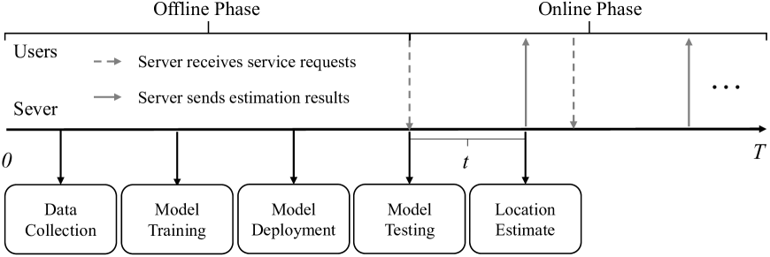
(a)

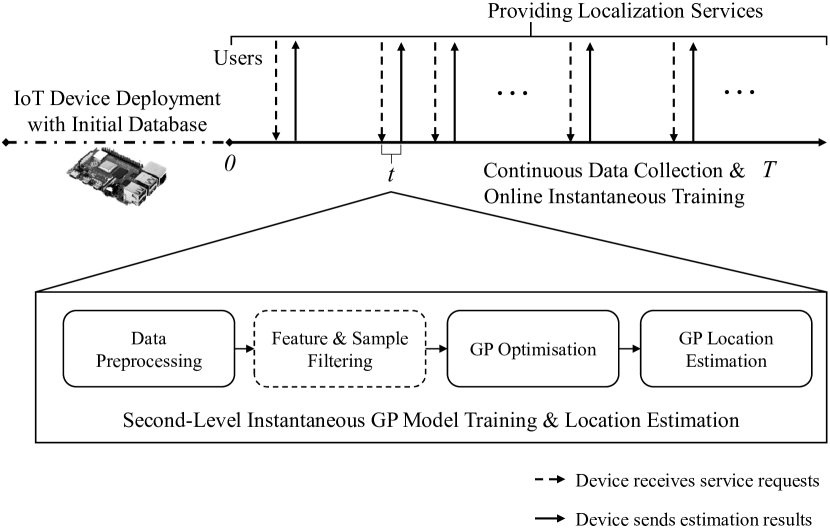
(b)

Figure 2: Comparison of (a) the conventional, two-phase indoor localization framework based on a centralized server and (b) the newly-proposed, decentralized indoor localization framework based on models deployed on IoT devices.

IV Experimental Results

To evaluate the performance and computational and data efficiency of the proposed indoor localization model based on SGP-RI, we carried out a series of experiments for both single-building and single-floor indoor localization with our own Xi’an Jiaotong-Liverpool University (XJTLU) dynamic database [32] and also the multi-building and multi-floor indoor localization with the publicly-available UJIIndoorLoc database [18].

For comparison with reference models under the conventional, two-phase indoor localization framework based on a centralized server, we run models on two distinct platforms: (1) a server equipped with an AMD Ryzen 7 5800X processor, an RTX 3060 Ti GPU, $16\text{\,}\mathrm{GB}$ of RAM, and $1\text{\,}\mathrm{TB}$ of storage, and (2) a Raspberry Pi 4B—as an IoT device—featuring a Cortex-A72 CPU, $4\text{\,}\mathrm{GB}$ of RAM, and $16\text{\,}\mathrm{GB}$ of storage.

As for the performance metrics, we adopted the following:

• 2D error: Two-dimensional localization error in single-building and single-floor indoor localization.

• 3D error: Three-dimensional localization error in multi-building and multi-floor indoor localization.

• Training time: Model training time on a given platform, which is related to the computational efficiency of a model.

• Model sparsity: Percentage ratio of the number of inducing points to the size of the training dataset (i.e., $100{\times}\frac{M}{N}$), which is related to the sparsity of SGP-RI model in approximating GP [29].

Note that the 2D and 3D Errors are related as follows:

$$\text{3D Error}=(1-h_{B})\times p_{B}+(1-h_{F})\times p_{F}+\text{2D Error},$$ (13)

where $h_{B}$ and $h_{F}$ are building and floor hit rates, and $p_{B}$ and $p_{F}$ are penalties for the errors in building and floor identification that are set to $50\text{\,}\mathrm{m}$ and $4\text{\,}\mathrm{m}$, respectively [18].

IV-A Single-Building and Single-Floor Indoor Localization

We select the XJTLU dynamic database [32] for the performance evaluation of localization models in single-building and single-floor indoor localization under dynamic as well as static scenarios, which covers three floors of the International Research Centre located on XJTLU South Campus, whose total area is $1200\text{\,}{\mathrm{m}}^{2}$. The Wi-Fi 2.4/5-$\mathrm{GHz}$ RSSI fingerprints in the database were measured at 101 RPs—i.e., 28, 35, and 38 RPs on the sixth, seventh, and eighth floors, respectively—spaced about $3\text{\,}\mathrm{m}$ from each other over 44 days by not only tens of surveyors using smartphones and laptops for daily measurements but also Raspberry Pi Pico Ws equipped with 2.4-$\mathrm{GHz}$ Wi-Fi interface deployed on the walls for hourly measurements as shown in Fig. 3; 466 WAPs had been detected during the whole measurement period. For the experiments, we split the XJTLU dynamic database into a training dataset based on the data measured during the first 24 days and a test dataset based on the data measured during the remaining 20 days.

Figure 3: RP distribution on the 7th floor of the XJTLU International Research Centre, where the RPs with Raspberry Pi Pico Ws are marked in red [32].

As for the proposed SGP-RI model, we use the Rational Quadratic (RatQuad) kernel [20] for all the experiments:

$$k(\bm{\mathbf{x}}_{i},\bm{\mathbf{x}}_{j})=\left(1+\frac{\|\bm{\mathbf{x}}_{i}-\bm{\mathbf{x}}_{j}\|^{2}}{2\alpha l^{2}}\right)^{-\alpha},$$ (14)

where $\alpha$ is the scale mixture parameter and $l$ is the length-scale [20], whose values are set to 2 and 10, respectively. Note that we can use different kernels with different parameter values for target floors to optimize the localization performance in actual deployment because the performance of GP/SGP-RI models highly depends on the choice of kernels and their parameter values.

For comparative analyses, we also consider reference models during the experiments. For NN-based models, we choose simplified CNN and DNN models tailored for classification, The structure and parameters of DNN and CNN received inspiration from [4] and [5]. Both use Stacked Auto Encoder (SAE) and use, as activation functions, Exponential Linear Unit (ELU) and Rectified Linear Unit (ReLU), respectively. The DNN includes 4 layers for classification (CLS) and the CNN uses Convolution for 1D (Conv1D), the network architectures are summarized in Tables I and II; simple adjustments were also made to take into account database differences. As for conventional algorithms, we consider $k$-Nearest Neighbors ($k$-NN) and Random Forests (RF) [33] for regression, where the number of neighbors for $k$-NN and the number of decision trees are set to 20 and 100, respectively.

TABLE I: DNN network architecture.

Layer	Activation Function	Parameters
SAE Encoder	ELU	465-232-116
SAE Decoder	ELU	116-232-465
CLS Layer 1	ELU	512
CLS Layer 2	ELU	512
CLS Layer 3	ELU	512
CLS Layer 4	ELU	512
Output Layer	-	35

TABLE II: CNN network architecture.

Layer	Description	Parameters
SAE Encoder	ReLU	465-232-116
SAE Decoder	ReLU	116-232-465
Conv1D Layer 1	ReLU	kernel size 22, output channel 99
Conv1D Layer 2	ReLU	kernel size 22, output channel 66
Flatten	-	-
Output Layer	-	35

IV-A1 Experiments Based on The Sever

Before evaluating the realistic performance of the models on the resource-constrained IoT device for the proposed, decentralized indoor localization framework, we first assess their absolute performance on the GPU server with plenty of computational resources for the conventional, two-phase and centralized indoor localization framework.

From the results summarized in Table III, we observe that the proposed SGP-RI model can strike the right balance between localization performance (i.e., 2D Error) and computational efficiency (i.e., Training Time), especially compared to the GP model. In the case of the SGP-RI model with the model sparsity of 25%, for example, we can reduce the training time of the GP model by nearly 75% at the slight increase of 2D error by about 8%, which is still better than those of NN-based models and conventional algorithms. Note that, though computationally highly efficient, RF and $k$-NN algorithms cannot provide decent localization performance unlike the SGP-RI model.

To gain a deeper insight into the error distribution, we generated both Cumulative Distribution Function (CDF) curves for the errors as shown in Fig. 4. Assuming a maximum error tolerance of $5\text{\,}\mathrm{m}$, it was observed that the probability of staying within this tolerance is only achieved when using inducing points larger than $25\%$. Also, the maximum value of the proposed model is less than $15\text{\,}\mathrm{m}$, while the other models have a maximum value of less than $25\text{\,}\mathrm{m}$.

TABLE III: Experimental results based on the server.

Model	2D Error [m]	Training Time [s]	Model Sparsity
GP	5.32	12.79	—
SGP-RI	5.80	6.08	50%
SGP-RI	5.96	5.52	40%
SGP-RI	6.44	5.00	30%
DNN	5.86	17.18*	—
CNN	5.87	12.06*	—
RF	7.00	1.11	—
$k$-NN	7.12	0.07	—

• GPU enabled.

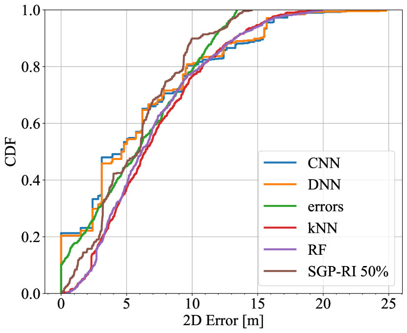
Figure 4: The CDF curve of the 2D Error of the experiment based on sever.

IV-A2 Experiments Based on The IoT System Device

To complete the experiments on IoT system devices, we used a Raspberry Pi 4B to simulate WAPs with redundant arithmetic in the IoT system. Due to the lack of powerful GPU on the Raspberry Pi 4B, we could not train and run the DNN and CNN models. Given the Raspberry Pi’s lack of active cooling and the risk of overheating during prolonged or consecutive testing, all the experiments were conducted in an environment maintained at approximately $25\text{\,}\mathrm{\SIUnitSymbolCelsius}$. Adequate time was allowed for the Raspberry Pi to cool to room temperature before subsequent testing commenced. Please note that fluctuations in training time are strongly influenced by temperature, so orders of magnitude of training time are meaningful, not exact times. In addition, if GP is deployed, a Raspberry Pi 4B with at least $64\text{\,}\mathrm{GB}$ of storage, and active cooling to ensure that operating temperatures are always below $50\text{\,}\mathrm{\SIUnitSymbolCelsius}$ is required, a condition that is inconsistent with other models mentioned in Section IV.

The experimental results based on the Raspberry Pi 4B are summarized in Table IV. Despite the low computational capability on the device, the proposed SGP-RI model successfully completed training within $30\text{\,}\mathrm{s}$ and delivered reliable accuracy. This demonstrates the algorithm’s efficacy in resource-constrained environments, such as IoT devices, where it can maintain efficiency and precision.

TABLE IV: Experimental results based on the IoT system device.

Model	2D Error [m]	Training Time [s]	Model Sparsity
GP*	5.44	96.34	—
SGP-RI	5.84	24.03	50%
SGP-RI	5.96	20.45	40%
SGP-RI	6.50	18.20	30%
RF	7.08	2.62	—
$k$-NN	7.10	1.17	—

• GP’s experiment equipment and requirements differ from those of other models as detailed in Section IV-A2.

IV-A3 Experiments Under A Dynamic Localization Scenario

As demonstrated by the experimental results in Section IV-A2, the real-time-trainability of the proposed SGP-RI model on IoT devices provides the continuous data collection and online instantaneous training under the proposed indoor localization framework shown in Figure 2 (b) and thereby enables the model to adapt to the dynamic and fluctuating indoor electromagnetic environment, which is not possible under the conventional, two-phase indoor localization framework based on a centralized server due to the prohibitive cost of retraining.

To demonstrate the advantage of the proposed indoor localization model and framework over the conventional ones, we simulated the following post-deployment scenario: For the DNN and CNN models, the training dataset is still based on the measurements during the first 24 days, but the test dataset is now divided into four groups of 5-day measurements each, for each of which we calculate the 2D error separately. For the SGP-RI, RF, and $k$-NN models, the initial training dataset is based on the measurements during the first 24 days, but the four groups of the test dataset are sequentially moved from the test dataset to the training dataset, which simulates those models operating under the proposed indoor localization framework based on frequent retraining with new sets of data over time. The results in Table V show that the proposed SGP-RI model provides the best 2D errors over the whole period thanks to its frequent retraining, highlighting its capability to maintain higher localization performance in spite of the environmental changes. It is this adaptability that differentiates the proposed indoor localization model and framework over the conventional ones.

TABLE V: 2D Errors under a dynamic localization scenario.

Model	2D Error for Each Test Period [m]
	1-5	6-10	11-15	16-20
DNN	5.58	5.77	5.96	6.12
CNN	5.72	5.82	6.05	5.89
SGP-RI	5.46	5.42	5.64	5.80
RF	6.76	6.66	6.81	6.82
$k$-NN	6.88	6.68	6.90	7.07

IV-B Multi-Building and Multi-Floor Indoor Localization

In Table VI, we summarize the performance of multi-building and multi-floor indoor localization of the proposed SGP-RI model with the model sparsity of 50% (i.e., “SGP-RI 50%”) as well as that of the reference models in the literature based on the UJIIndoorLoc database, which is the first publicly-available multi-building and multi-floor Wi-Fi RSSI fingerprint database covering the three multi-floor buildings on the University Jaume I (UJI) campus in Castelló de la Plana, Spain [18].

The results in Table VI indicate that the proposed SGP-RI model can also provide indoor localization performance comparable to that of the state-of-the-art models under a multi-building and multi-floor environment.

Note that the 3D errors listed in Table VI should be interpreted as relative indicators of the models’ performance because they are not calculated under the same condition as frequently discussed in the literature (e.g., [4, 27]): The top four models from the 2015 EvAAL/IPIN competition [34] are evaluated based on the training, validation, and test datasets of the UJIIndoorLoc database, the last of which, however, is not publicly available. Therefore, the rest of the models are evaluated based only on the training and validation datasets of the UJIIndoorLoc database.

Also, the calculation of the 3D error under the new decentralized indoor localization framework based on the SGP-RI models deployed on IoT devices is different from that under the conventional, two-phase indoor localization framework based on a model running on a centralized server. Unlike the conventional framework, the proposed framework uses a single IoT device for location service covering a whole or part of a floor, whose location is known during its deployment. Under this decentralized framework, it is assumed that the estimation of the building and floor is based on the RSSIs from IoT devices measured at a user’s device, where the strongest-RSSI IoT device can provide the building and floor information of a user. Considering a large attenuation of Wi-Fi signals from different buildings, we set $h_{B}$, the building hit rate, to 1, which is more or less consistent with the building estimation performance of the state-of-the-art centralized models. As for $h_{F}$, the floor hit rate, it is reasonable to assume that an IoT devices with the strongest-RSSI is located at the same floor as the user or its neighboring floors. Determining $h_{F}$ in a multi-building, multi-floor environment, therefore, can be transformed into a binary (i.e., top and bottom floors) or ternary (i.e., all other floors) classification task. We designed a simple $k$-NN with $k{=}7$ to accomplish the classification task and evaluated the value of $h_{F}$ using the UJIIndoorLoc database, whose average is 80%. More advanced and complex classification algorithms likely result in higher $h_{F}$ values, of course, but it is not feasible for resource-constrained IoT devices.

TABLE VI: Location estimation error based on the UJIIndoorLoc database

	Model	3D Error [m]
EvAAL IPIN 2015 [36]	RTLS@UM	6.20
	ICSL	7.67
	HFTS	9.49
	MOSAIC	11.64
	SGP-RI 50%	6.87
	CDAELoc [35]	7.37
	SALLoc [37]	8.28
	EA-CNN [38]	8.34
	RNN-MOGP Aug [27]	8.42
	RNN [6]	8.62
	CHISEL [39]	8.80
	DNN-DLB [40]	9.07
	Scalable DNN [4]	9.29
	CNNLoc [5]	11.78
	CCpos [41]	12.4

V Conclusions

In this paper we have proposed a real-time-trainable and decentralized IoT indoor localization model based on SGP-RI, which significantly reduces the computational complexity of a GP-based model and thereby can be deployed to, and run on, a resource-constrained IoT system device.

The experimental results, based on both dynamic and static Wi-Fi fingerprint databases, demonstrate the feasibility of the SGP-RI model under the newly-proposed, decentralized indoor localization framework, enabling frequent retraining of deployed models with updated databases to better adapt to the dynamic and fluctuating indoor electromagnetic environment, which is not possible under the conventional, two-phase indoor localization framework based on a centralized server due to the prohibitive cost of retraining. Specifically, the experimental results show that the SGP-RI model can provide comparable localization performance using only a fraction of the entire training dataset with reduced dimensionality and spending less training time. Thanks to its real-time-trainability, the SGP-RI model also exhibits superior long-term stability and resilience to environmental dynamics compared to the conventional, centralized models.

Though we focus on the real-time-trainable IoT indoor localization model based on SGP-RI, it is just our first attempt to enable the decentralized indoor localization framework based on models deployed on IoT devices, which integrates the two separate operational phases of the conventional centralized framework into a unified workflow to provide continuous data collection and online instantaneous training for better adaptation to the time-varying statistics of Wi-Fi RSSI fingerprints. The new indoor localization framework is also suitable for IoT ecosystems, which have been being deployed in the field and integrated into existing Wi-Fi infrastructure, mostly based on centrally-managed WAPs. The proposed framework reduces reliance on a centralized server, which could be a single point of failure, and thereby mitigates service disruptions caused by malicious attacks. This is achieved through multiple models running on IoT devices covering only target floors of the whole service area. It is also important to note that the same IoT devices can be used to automatically collect Wi-Fi RSSI fingerprints as well, which is the case for the construction of our own XJTLU dynamic database [42] and provides a promising solution for the maintenance and update of the Wi-Fi fingerprint databases [43].

Improving the WAP-based feature selection for input dimensionality reduction and the RP-based inducing point selection could be an interesting topic for future work. It is also worth investigating a hybrid indoor localization framework utilizing a centralized server and multiple IoT devices running real-time-trainable models together in order to get the benefits of both centralized and decentralized indoor localization frameworks.

References

- [1] T. Yang, A. Cabani, and H. Chafouk, “A survey of recent indoor localization scenarios and methodologies,” Sensors, vol. 21, no. 23, 2021, (article number: 8086).
- [2] W. Liu, Y. Zhang, Z. Deng, and H. Zhou, “Low-cost indoor wireless fingerprint location database construction methods: A review,” IEEE Access, vol. 11, pp. 37 535–37 545, 2023.
- [3] Y. Tao, L. Zhao, Q. Zhang, and Z. Chen, “Wi-Fi fingerprint database refinement method and performance analysis,” in Proc. 2018 Ubiquitous Positioning, Indoor Navigation and Location-Based Services (UPINLBS), 2018, pp. 1–6.
- [4] K. S. Kim, S. Lee, and K. Huang, “A scalable deep neural network architecture for multi-building and multi-floor indoor localization based on Wi-Fi fingerprinting,” Big Data Analytics, vol. 3, no. 1, Apr 2018. [Online]. Available: http://dx.doi.org/10.1186/s41044-018-0031-2
- [5] X. Song, X. Fan, C. Xiang, Q. Ye, L. Liu, Z. Wang, X. He, N. Yang, and G. Fang, “A novel convolutional neural network based indoor localization framework with WiFi fingerprinting,” IEEE Access, vol. 7, pp. 110 698–110 709, 2019.
- [6] A. E. Ahmed Elesawi and K. S. Kim, “Hierarchical multi-building and multi-floor indoor localization based on recurrent neural networks,” in Proc. 2021 Ninth International Symposium on Computing and Networking Workshops (CANDARW), 2021, pp. 193–196.
- [7] S. M. Nguyen, D. V. Le, and P. J. Havinga, “Seeing the world from its words: All-embracing transformers for fingerprint-based indoor localization,” Pervasive and Mobile Computing, vol. 100, p. 101912, 2024.
- [8] S. Wang, S. Zhang, J. Ma, and O. A. Dobre, “Graph neural network-based wifi indoor localization system with access point selection,” IEEE Internet of Things Journal, pp. 1–1, 2024.
- [9] N. Savin, “Exploring indoor localization with transformer-based models: A CNN-transformer hybrid approach for WiFi fingerprinting,” July 2023. [Online]. Available: http://essay.utwente.nl/96104/
- [10] “OpenWrt - Welcome to the OpenWrt Project, url = https://openwrt.org/start.”
- [11] K. Venkatesh, P. Rajkumar, S. Hemaswathi, and B. Rajalingam, “IoT based home automation using raspberry Pi,” J. Adv. Res. Dyn. Control Syst, vol. 10, no. 7, pp. 1721–1728, 2018.
- [12] Z. Kasmi, N. Guerchali, A. Norrdine, and J. H. Schiller, “Algorithms and position optimization for a decentralized localization platform based on resource-constrained devices,” IEEE Transactions on Mobile Computing, vol. 18, no. 8, pp. 1731–1744, 2019.
- [13] N. Garg and N. Roy, “Sirius: A self-localization system for resource-constrained IoT sensors,” in Proc. 21st Annual International Conference on Mobile Systems, Applications and Services, 2023, pp. 289–302.
- [14] A. Christidis, R. Davies, and S. Moschoyiannis, “Serving machine learning workloads in resource constrained environments: a serverless deployment example,” in in Proc. 2019 IEEE 12th Conference on Service-Oriented Computing and Applications (SOCA), 2019, pp. 55–63.
- [15] B. Sliwa, N. Piatkowski, and C. Wietfeld, “Limits: Lightweight machine learning for IoT systems with resource limitations,” in Proc. 2020 IEEE International Conference on Communications (ICC), 2020, pp. 1–7.
- [16] F. Zhou, K. Lin, A. Ren, D. Cao, Z. Zhang, M. U. Rehman, X. Yang, and A. Alomainy, “RSSI indoor localization through a bayesian strategy,” in Proc. 2017 IEEE 2nd Advanced Information Technology, Electronic and Automation Control Conference (IAEAC), 2017, pp. 1975–1979.
- [17] V. Moghtadaiee and A. G. Dempster, “Design protocol and performance analysis of indoor fingerprinting positioning systems,” Physical Communication, vol. 13, pp. 17–30, 2014.
- [18] J. Torres-Sospedra, R. Montoliu, A. Martínez-Usó, J. P. Avariento, T. J. Arnau, M. Benedito-Bordonau, and J. Huerta, “UJIIndoorLoc: A new multi-building and multi-floor database for WLAN fingerprint-based indoor localization problems,” in Proc. 2014 International Conference on Indoor Positioning and Indoor Navigation (IPIN), 2014, pp. 261–270.
- [19] W. Njima, M. Chafii, A. Chorti, R. M. Shubair, and H. V. Poor, “Indoor localization using data augmentation via selective generative adversarial networks,” IEEE Access, vol. 9, pp. 98 337–98 347, 2021.
- [20] C. E. Rasmussen and C. K. I. Williams, Gaussian Processes for Machine Learning, ser. Adaptive Computation and Machine Learning. MIT Press, 2006.
- [21] D. Tran, R. Ranganath, and D. M. Blei, “The variational gaussian process,” arXiv preprint arXiv:1511.06499, 2015.
- [22] A. Uddin, X. Tao, C.-C. Chou, and D. Yu, “Are missing values important for earnings forecasts? A machine learning perspective,” Quantitative finance, vol. 22, no. 6, pp. 1113–1132, 2022.
- [23] L. O. Joel, W. Doorsamy, and B. S. Paul, “A review of missing data handling techniques for machine learning,” International Journal of Innovative Technology and Interdisciplinary Sciences, vol. 5, no. 3, pp. 971–1005, 2022.
- [24] S. García, J. Luengo, and F. Herrera, Data preprocessing in data mining. Springer, 2015, vol. 72.
- [25] T. Emmanuel, T. Maupong, D. Mpoeleng, T. Semong, B. Mphago, and O. Tabona, “A survey on missing data in machine learning,” Journal of Big data, vol. 8, pp. 1–37, 2021.
- [26] M. K. Hasan, M. A. Alam, S. Roy, A. Dutta, M. T. Jawad, and S. Das, “Missing value imputation affects the performance of machine learning: A review and analysis of the literature (2010–2021),” Informatics in Medicine Unlocked, vol. 27, p. 100799, 2021.
- [27] Z. Tang, S. Li, K. S. Kim, and J. S. Smith, “Multi-dimensional Wi-Fi received signal strength indicator data augmentation based on Multi-Output Gaussian Process for large-scale indoor localization,” Sensors, vol. 24, no. 3, 2024, (article number: 1026). [Online]. Available: https://www.mdpi.com/1424-8220/24/3/1026
- [28] J. Quinonero-Candela and C. E. Rasmussen, “A unifying view of sparse approximate gaussian process regression,” The Journal of Machine Learning Research, vol. 6, pp. 1939–1959, 2005.
- [29] E. Snelson and Z. Ghahramani, “Sparse gaussian processes using pseudo-inputs,” in Advances in Neural Information Processing Systems, Y. Weiss, B. Schölkopf, and J. Platt, Eds., vol. 18. MIT Press, 2005.
- [30] J. Nocedal, “Updating quasi-newton matrices with limited storage,” Mathematics of computation, vol. 35, no. 151, pp. 773–782, 1980.
- [31] S. Li, Z. Tang, K. S. Kim, and J. S. Smith, “Exploiting unlabeled rssi fingerprints in multi-building and multi-floor indoor localization through deep semi-supervised learning based on mean teacher,” in Proc. CANDAR 2023, 2023, pp. 155–160, outstanding paper award.
- [32] Z. Tang, R. Gu, S. Li, K. S. Kim, and J. S. Smith, “Static vs. dynamic databases for indoor localization based on Wi-Fi fingerprinting: A discussion from a data perspective,” in Proc. 2024 International Conference on Artificial Intelligence in Information and Communication (ICAIIC), 2024, pp. 760–765.
- [33] P. Geurts, D. Ernst, and L. Wehenkel, “Extremely randomized trees,” Machine Learning, vol. 63, pp. 3–42, 2006.
- [34] A. Moreira, M. J. Nicolau, F. Meneses, and A. Costa, “Wi-Fi fingerprinting in the real world - RTLS@UM at the EvAAL competition,” in 2015 International Conference on Indoor Positioning and Indoor Navigation (IPIN). IEEE, pp. 1–10. [Online]. Available: http://ieeexplore.ieee.org/document/7346967/
- [35] P. Zhou, H. Wang, R. Gravina, and F. Sun, “WIO-EKF: Extended kalman filtering-based Wi-Fi and inertial odometry fusion method for indoor localization,” IEEE Internet of Things Journal, pp. 1–1, 2024.
- [36] A. Moreira, M. J. a. Nicolau, F. Meneses, and A. Costa, “Wi-Fi fingerprinting in the real world - RTLSUM at the EvAAL competition,” in Proc. 2015 International Conference on Indoor Positioning and Indoor Navigation (IPIN), 2015, pp. 1–10.
- [37] S. L. Ayinla, A. A. Aziz, and M. Drieberg, “SALLoc: An accurate target localization in WiFi-Enabled indoor environments via SAE-ALSTM,” IEEE Access, vol. 12, pp. 19 694–19 710, 2024.
- [38] A. Alitaleshi, H. Jazayeriy, and J. Kazemitabar, “EA-CNN: A smart indoor 3D positioning scheme based on Wi-Fi fingerprinting and deep learning,” Engineering Applications of Artificial Intelligence, vol. 117, p. 105509, 2023.
- [39] L. Wang, S. Tiku, and S. Pasricha, “Chisel: compression-aware high-accuracy embedded indoor localization with deep learning,” IEEE Embedded Systems Letters, vol. 14, no. 1, pp. 23–26, 2021.
- [40] M. Laska and J. Blankenbach, “Deeplocbox: Reliable fingerprinting-based indoor area localization,” Sensors, vol. 21, no. 6, 2021, (article number: 2000). [Online]. Available: https://www.mdpi.com/1424-8220/21/6/2000
- [41] F. Qin, T. Zuo, and X. Wang, “Ccpos: Wifi fingerprint indoor positioning system based on cdae-cnn,” Sensors, vol. 21, no. 4, p. 1114, 2021.
- [42] Z. Zhong, Z. Tang, X. Li, T. Yuan, Y. Yang, W. Meng, Y. Zhang, R. Sheng, N. Grant, C. Ling, X. Huan, K. S. Kim, and S. Lee, “XJTLUIndoorLoc: A new fingerprinting database for indoor localization and trajectory estimation based on Wi-Fi RSS and geomagnetic field,” in Proc. CANDAR’18, Hida Takayama, Japan, Nov. 2018.
- [43] S. Li, Z. Tang, K. S. Kim, and J. S. Smith, “On the use and construction of Wi-Fi fingerprint databases for large-scale multi-building and multi-floor indoor localization: A case study of the UJIIndoorLoc database,” Sensors, vol. 24, no. 12, 2024, (article number: 3827). [Online]. Available: https://doi.org/10.3390/s24123827