HiFAKES: High-frequency synthetic appliance signatures generator for non-intrusive load monitoring
Abstract
The increasing number of electrical appliances in households and the need to reduce energy costs for consumers have led to the growing importance of non-intrusive load monitoring (NILM), or energy disaggregation systems to manage energy efficiency. These systems rely on data-driven methods and require extensive datasets of power consumption over a long period of time. However, the scarcity of datasets negatively impacts the performance of current NILM algorithms. Further, while the vast majority of these datasets are made by collecting low-frequency sampling power consumption patterns, high-frequency datasets, which would significantly improve the accuracy of load identification, are comparatively few due to the time and costs that such data collection entail. As a response to these problems, synthetic datasets have been developed. Existing synthetic datasets for NILM, while useful, typically depend on large training datasets and are evaluated using a single aggregated test metric, which cannot precisely reflect the fidelity, diversity, and novelty of the data. To address this gap, we introduce HiFAKES, a novel physics-informed, training-free generative model designed to produce high-frequency sampling synthetic power signatures. HiFAKES generates synthetic data with superior fidelity and diversity. Indeed, the -precision and -recall indicators are respectively about 2.5 times larger than those for existing models, this makes our proposed model highly effective for NILM applications. HiFAKES operates by generating reference signatures templates based on real appliance signatures data, and by replicating these with some features variations, thus simulating both known and novel appliances. A key advantage of this model is its ability to generate unlimited high-frequency synthetic appliance data from a single training example. The generated data closely mimics real-world power consumption, as demonstrated by comprehensive evaluations, including the so-called 3D metric (-precision, -recall, authenticity) and domain classifier tests. Our generative model HiFAKES is a plug-and-play tool that requires minimal computational resources, thus significantly enhancing synthetic data generation for NILM.
keywords:
NILM , energy disaggregation , power consumption, data analytics, synthetic data, high-frequency dataset, energy in buildings[inst1]department=Center for Digital Engineering,, organization=Skolkovo Institute of Science and Technology,addressline=30 Bolshoy Boulevard, city=Moscow, postcode=121205, country=Russia
[inst2]organization=Monisensa Development LLC,city=Moscow, country=Russia
1 Introduction
The integration of new appliances into daily life, combined with rising electricity costs, is prompting more households to optimize their energy consumption [1, 2]. One effective strategy for optimization is identifying and modifying inefficient behavioral habits that consumers may not be aware of [3]. Providing detailed information on energy usage — ideally at the appliance level — empowers consumers to make informed decisions and take conscious actions to manage their consumption patterns more effectively. Achieving this requires appliance-level monitoring, which can be done either intrusively by installing sensors on each appliance (sub-metering) or non-intrusively from a single metering point [4]. Compared to sub-metering, non-intrusive load monitoring (NILM) is a cost-effective solution that can seamlessly integrate into daily routines and offer valuable feedback to consumers [5].
NILM is a data-driven method for analyzing a household’s total energy consumption to identify active appliances, estimate their energy usage, and detect potential malfunctions [6, 7]. NILM algorithms rely heavily on the availability of comprehensive datasets that include a broad and diverse range of appliances, each with various power consumption patterns. The more extensive and varied these datasets, the more effectively NILM algorithms can identify and analyze appliances usage. NILM typically uses two types of datasets: low- and high-frequency sampling datasets of appliances power consumption signatures [8]. High-frequency datasets provide maximal informational content which can significantly improve the load identification in NILM algorithms [9, 10, 11]. However, collecting such data, especially high-frequency datasets, requires sophisticated hardware and often takes years of data collection. As a result, synthetic data generation has become a fast and reliable alternative.
Synthetic data is the data artificially produced by a generative model, and intends to mimic patterns and the structure of the real data. In the context of appliance power consumption data, they can create realistic synthetic appliance signatures for testing and validating new NILM algorithms under different scenarios, which is particularly useful when real data collection is challenging as it is for high-frequency sampling datasets. So far, only five works exist that have attempted to develop synthetic data generators for NILM: SmartSim [12], AMBAL [13], SHED [14], SynD [15], and PIASG [16]. Among these, SHED and PIASG are designed for both low- and high-frequency data, whereas SmartSim, AMBAL, and SynD are focused exclusively on low-frequency data.
When developing synthetic datasets for NILM, several key points must be addressed: First, how closely the synthetic samples resemble the features of their real-world counterparts (fidelity); Second, if the synthetic dataset offers a variety that truly reflects the full range of real data (diversity); whether the model generates novel, unseen data rather than merely replicating existing samples (generalization/novelty). Fidelity, diversity and generalization are three criteria that need to be optimized simultaneously to ensure the generation of high-quality synthetic datasets.
Existing models tend to combine these criteria into a single evaluation metric, which does not allow for a clear, individual assessment of each criterion and makes the evaluation less interpretable. Moreover, the use of different evaluation metrics further complicates the comparison of these datasets. For instance, some models use distributional similarity metrics such as the Hellinger distance in SynD and Kullback-Leibler divergence in PIASG. These metrics do not explicitly evaluate fidelity, diversity, or novelty individually but instead aggregate them into a single score. Similarly, AMBAL employs the mean absolute percentage error, and SHED visually compares distributions based on autocorrelation, kurtosis, entropy, Laplace scale parameter, and total harmonic distortion (THD). SmartSim, on the other hand, uses metrics such as the F1-score, normalized error in assigned power, and Matthews correlation coefficient to evaluate NILM algorithms trained on their synthetic dataset. While these metrics assess algorithmic performance, they do not directly measure the quality of the synthetic data itself.
In this work, we propose HiFAKES, a novel generative model for NILM data specifically designed to optimize fidelity, diversity, and generalization. HiFAKES is a physics-informed, one-shot generative model capable of producing high-fidelity and diverse signatures for both known and unseen appliances. Our primary contributions are as follows:
-
1.
We conducted a comprehensive analysis of high-frequency real-world datasets, revealing that appliance signatures can be constructed from the two components that we call instantaneous states and amplitude envelopes. This insight has significantly simplified the process of generating power consumption signatures, allowing for gradual modifications of their components — instantaneous states and amplitude envelopes.
-
2.
We developed HiFAKES, a novel physics-informed, one-shot generative model that uses a single training example to produce unlimited high-frequency synthetic appliance data, eliminating the need for extensive training.
-
3.
We presented a seamless and compact theoretical framework that ensures the transparency and reproducibility of the HiFAKES generative model.
-
4.
To the best of our knowledge, for the first time in the field of NILM, we used state-of-the-art domain-agnostic metrics: -precision, -recall, and authenticity to evaluate the fidelity, diversity and generalization of the existing high-frequency synthetic datasets and the one produced by HiFAKES.
-
5.
We achieved up to 2.76 times superior fidelity and 2.5 times superior diversity of the high-frequency datasets generated by HiFAKES compared to the existing generative models for NILM.
-
6.
We made the GitHub repository containing the Python source-code for HiFAKES available for public-access via this link.
The article is organized as follows: Section 2 provides a thorough literature review on existing generative models used in NILM. Section 3 provides an overview of related works, specifically focusing on the existing models for generating high-frequency data. In Section 4, first we provide detail analysis on high frequency data, and the underlying physical principles. Following this, we introduce HiFAKES, our proposed model, elaborating on its novel features, theoretical framework, and implementation details. In Section 5, we present a comprehensive evaluation of HiFAKES, detailing the 3D metric test and domain classifier test. Finally, Section 6 discusses the results, provides a comparative analysis with existing models, and concludes the paper outlining potential future work.
2 Literature review
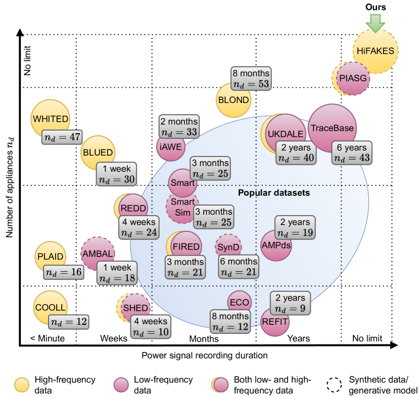
Datasets are essential for advancing NILM research by providing the data necessary for model development and evaluation. Publicly-available datasets for NILM, collected from [17, 18], are shown in Fig. 1, where they are categorized by the number of devices () they monitor and the longest duration of a power consumption signal recording. Notably, a few datasets, such as BLOND [19], WHITED [20], COOLL [21], PLAID [22], and BLUED [23], offer high-frequency data for appliances.
At present, only five synthetic datasets are available for NILM: SynD, AMBAL, and SmartSim, which are designed for low-frequency data, and SHED and PIASG, which generate both high and low-frequency data.
Beyond differences in sampling frequency, synthetic datasets for NILM, like other generative models, can be distinguished based on the amount of data they use and the amount of physical information they incorporate. Generally, there are three types of generative models: data-driven, physics-informed, and physics-based, as depicted in Fig. 2.
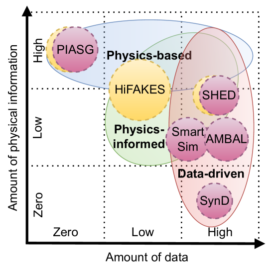
Data-driven generative models primarily depend on large datasets, and they focus on learning patterns from the data. Physics-informed generative models integrate physical principles for their implementation and interpretability. Physics-based generative models principally rely on mathematical models, regardless of the amount of data, but they can only be used when the whole physical process is known [25]. In Fig. 2, we categorized the six synthetic datasets for NILM, including HiFAKES, within this framework to better understand the strengths and limitations of existing works.
SynD is considered a purely data-driven generative model, while SmartSim, AMBAL, and SHED are classified as physics-informed models, and PIASG is categorized as a physics-based model. SmartSim and AMBAL fit predefined appliance models, such as the ON/OFF and ON/OFF Decay/Growth models, to real data. AMBAL is trained on the ECO [26] and Tracebase [27] datasets, while SmartSim is trained on the Smart* [28] dataset. Similarly, SHED employs a universal appliance model that is fitted to three real-world datasets (PLAID, COOLL, and Tracebase). Although the authors of PIASG describe their model as physics-informed, our analysis indicates that it does not utilize real data for generating new signatures but relies solely on a mathematical model. Thus, we classify this model as physics-based. The figure shows that all models, except PIASG, still require substantial real-world data for training. Finally, we categorize our proposed model, HiFAKES, as physics-informed and position it within the current landscape. As illustrated, HiFAKES maximizes the integration of physical information while minimizing dependence on extensive training data compared to the existing physics-informed generative models.
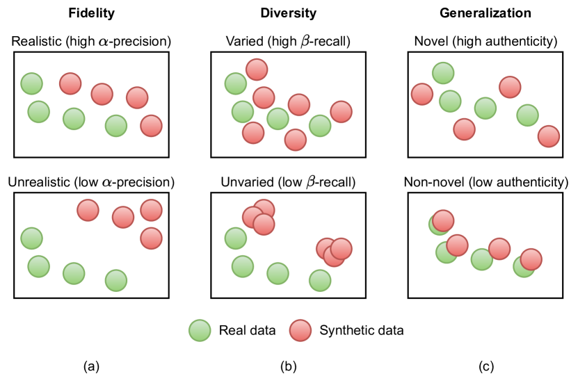
While categorizing these models helps to understand their applicability for NILM, it is crucial to evaluate and compare their quality using universal and interpretable metrics. It must be noted that only high-quality synthetic datasets can effectively substitute for real data in training robust and accurate models. Three key criteria can be used to evaluate the quality of generative models for synthetic datasets: Fidelity, Diversity, and Generalization [29], as illustrated in Fig. 3.
Fidelity
This criterion shows the level of realism and evaluates whether synthetic data points can be easily distinguished from real ones. Noticeable differences indicate that the synthetic data is unrealistic and has lower fidelity. As indicated in Fig. 3(a), the realistic synthetic data preserves the underlying distributions and relationships of the original data.
Diversity
In synthetic datasets, diversity is closely related to the variance of an underlying distribution. A diverse synthetic dataset should exhibit similar variance to that of the real dataset, ensuring that it accurately represents the range of values and the spread of the data. For instance, in Fig. 3(b), in the lower plot, the synthetic data points are overly concentrated in specific areas forming dense clusters, whereas the real ones are not. In this case, the generator fails to capture the broad range of patterns, and values found in the real data.
Generalization
This third criterion evaluates the model’s ability to generate novel data points that extend beyond the original data. This ensures that the synthetic data points are new observations and not mere copies of the training data. As illustrated in Fig. 3, dataset with high novelty have several unique points that are not existing in the real dataset but still follow the same distribution. Synthetic datasets with high novelty can significantly enhance a model’s ability to generalize to unseen real-world data.
However, until recently there were no domain-agnostic (universal) method to assess synthetic datasets with these key criteria as most of the existing evaluation metrics were tailored for synthetic images. In [29] an interpretable probabilistic three-dimensional metric was proposed based on precision-recall analysis [31]: -precision, -recall, and authenticity. This metric enabled comparison of synthetic datasets across various domains. The qualitative interpretation of these three metrics is also indicated in Fig. 3.
Another method to assess the quality of a synthetic dataset is by conducting domain classifier test [32]. The idea is to train a machine learning model to distinguish between real and synthetic signatures. For a high-quality synthetic dataset, it is expected that the model is unable to correctly classify with high confidence both synthetic and real signatures. This evaluation reveals how effectively the synthetic data replicates the hidden characteristics of real-world data. It is important to note that this test is not a replacement for the previously discussed metrics, but rather an additional validation step to confirm the reliability and applicability of synthetic datasets in real-world applications.
3 Overview of related works
Our focus is on a detailed examination of SHED and PIASG as of all the synthetic datasets for NILM, only these two models generate high-frequency data.
The synthetic high-frequency energy disaggregation (SHED) dataset provides a comprehensive generative model for both low- and high-frequency electrical signatures, specifically tailored for commercial buildings. Its methodology involves decomposing appliance electrical current signatures using a semi-non-negative matrix factorization algorithm into a predetermined number of components. This number is chosen to ensure that the signal-to-noise ratio between the actual signature and the residual (the difference between the real and reconstructed signatures) exceeds 50 dB, indicating high-quality reconstruction. The synthetic signatures are then generated by adding Gaussian noise to the reconstructed signatures. This approach facilitates the creation of high-frequency datasets that closely mimic real-world conditions. However, a notable limitation of SHED is its reliance on large training data, which restricts its ability to generate signatures for novel appliances not included in the training set. Additionally, SHED does not directly validate individual appliance signatures. Instead, the total current consumption of the simulated building, computed as the sum of the synthetic signatures, is compared with real-world datasets employing statistical metrics such as auto-correlation, kurtosis, entropy, and total harmonic distortion. This approach leaves ambiguity regarding which properties of the synthetic dataset—fidelity, diversity, or generalization—were specifically validated. Without direct validation of individual appliance signatures, it is unclear how accurately the synthetic data represents the nuanced behaviors of different appliances.
In PIASG, two generative, physics-informed models designed to simulate appliance signatures for both low- and high-frequency NILM datasets were introduced. These models utilize prior knowledge of the physical properties of appliance power consumption to create realistic synthetic data. High-frequency signatures are generated using a mathematical model that incorporates characteristics such as exponential decay of harmonics, phase changes between and radians, variations in the spectrum of AC cycles over time, and exponential decay of transient processes. The core idea involves randomly sampling sets of parameters that control these characteristics, with each set corresponding to a unique synthetic appliance. These parameters are then used as location parameters for predefined statistical distributions (e.g., normal, half-normal). From these distributions, parameters for a predefined number of appliance signatures are sampled. The sampled parameters are then substituted into the universal mathematical model for an appliance to produce authentic appliance signatures. This approach offers significant advantages, including transparent and intuitive control over underlying distributions, the ability to simulate a diverse range of appliances without requiring input data or a training process, and flexibility in generating signatures at different sampling frequencies. Its main limitation is that it is based on a simplified mathematical model, which, while accurately describing publicly available real-world signatures, may not generalize well to other datasets. From an evaluation perspective, the PIASG generative model was validated by comparing synthetic data with real data from public datasets using metrics such as the Kullback-Leibler (KL) divergence to measure the distributional similarity. However, similarly to previous works like SHED, this evaluation does not provide specific values for any of the three criteria—fidelity, diversity, or generalization—but rather offers an aggregated assessment of similarity.
4 Methodology
4.1 Analysis of high-frequency data
High-frequency appliance signatures typically resemble the AC voltage and current consumption patterns illustrated in Fig. 4. These power signatures are sampled above the Nyquist frequency, usually at rates ranging from 1 to 60 kHz. It is important to note that measuring the entire appliance duty cycle at these high sampling frequencies provides maximal informational content, which makes it very promising for NILM applications. Such signatures typically reveal appliance programs (see Figs. 4(g-i)) that correspond to different power consumption regimes (Figs. 4(d-f)), each designed to operate in a specific order. For demonstration purposes, we use short programs, defined as intervals of time during which one regime transitions to another. In this study, we focus on the analysis of AC current consumption as the primary indicator of power consumption patterns.
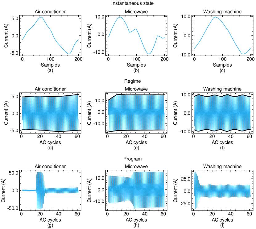
Before designing HiFAKES, we observed that the power consumption patterns of appliance operational modes can be effectively reconstructed using two fundamental components which we call here instantaneous states and amplitude envelopes. The instantaneous state characterizes the power consumption pattern within a single AC cycle, representing the electrical components in use by the appliance at a specific moment (as shown in Figs. 4(a-c)). In contrast, the amplitude envelope illustrates the variation in amplitude across consecutive AC cycles (see black solid lines in Figs. 4(d-f)). The architecture of HiFAKES is based on the two components mentioned above as it simplifies the generative process while enhancing its interpretability through their gradual modifications. In this work, the amplitude envelope is treated as a dimensionless quantity, while the instantaneous state is quantified in amperes, reflecting its direct relationship with electrical current. This is required to ensure consistency when multiplying physical dimensions of the instantaneous state and amplitude envelope.
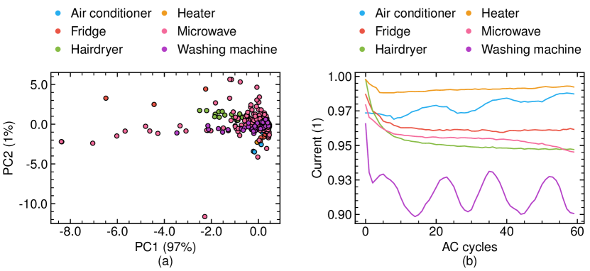
In our analysis of amplitude envelopes derived from real-world data, specifically the PLAID dataset, we employed principal component analysis (PCA) to examine their distribution, as illustrated in Fig. 5(a). The amplitude envelopes were defined by the maximum absolute value of each AC cycle within the power signature of the operational regime. The envelopes’ amplitudes were scaled to 1 prior to PCA. Our results indicate that a single principal component captures 97% of the variance in the original dataset, implying that this component is sufficient for reconstructing the amplitude envelopes. The majority of envelopes display an exponentially decaying pattern, with some converging to a steady state, as observed in appliances like heaters and fridges, while others oscillate around a steady state, as seen in appliances such as washing machines (see Fig. 5(b)). Notably, the amplitude envelope of an air conditioner exhibited oscillating growth over time.
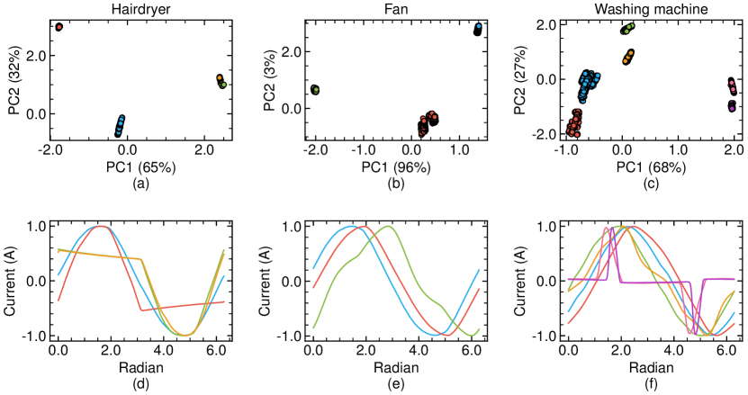
As to AC cycles, we also applied PCA to examine how different operations of the same appliance are reflected in their power signatures. As expected, appliances performing multiple operations generate power signatures that form distinct clusters as shown in Fig. 6. A visual inspection of principal components plotted in a 2D plane reveals that most instantaneous states form dense, convex clusters. One reason for the clusters’ convexity is that a measurement system has imperfections as measuring the power consumption signature of the same device under different conditions often results in slightly different signatures. Whereas this could be true for all the devices, the other reason for the observed convexity is the way how a particular appliance works. For instance, a laptop charger has variations in power consumption based on the workload of its main components such as central processing unit (CPU) and graphical processing unit. Consequently, we used the density-based spatial clustering algorithm of applications with noise (DBSCAN) to automatically identify those clusters. The results indicate that complex devices, such as hairdryers, fans, and washing machines, can have up to six different states. For instance, one washing machine signature (Fig. 6(f)) resembles that of laptop chargers, which is corresponding to the standby mode of the washing machine. The remaining washing machine signatures can be associated with various regimes such as spinning or rinsing.
4.2 HiFAKES: high-frequency synthetic appliance signatures generator
HiFAKES is a physics-informed, one-shot generative model designed to simulate high-frequency signatures for both known and unseen appliances. By physics-informed, we mean that the model seamlessly integrates prior data and physics-based rules. This also includes insights from our analysis of high-frequency data, see Section 4.1. The term one-shot indicates that the model can generate synthetic data from only a single training example given.
4.2.1 Architecture overview
Several key physical principles are embedded within HiFAKES: (i) a program signature can be decomposed into regime signatures; (ii) each regime signature can further be broken down into instantaneous states and amplitude envelopes; (iii) an instantaneous state can be expressed as a linear combination of other states, known or unknown. The principle is consistent with circuit theory, where the current consumption of different components contributes to the aggregate signal of the circuit; and (iv) the instantaneous states and amplitude envelopes associated with a particular regime form convex clusters like those shown in Fig. 6(a-c).
The model operates under the following assumptions: (i) the voltage waveform is purely sinusoidal; (ii) each AC cycle maintains a fixed frequency, indicating no frequency fluctuations; (iii) all AC cycles are synchronized with the ideal voltage at the zero phase; (iv) the current may exhibit jump discontinuities.
The ability to design a one-shot generative model largely stems from these physical principles. Specifically, the idea is that the instantaneous state and amplitude envelope derived from a real appliance signature can be projected in various directions to generate synthetic appliance signatures. This projection essentially involves creating linear combinations of harmonics, in line with principle (iii). The same logic applies to amplitude envelopes, as they are derived from sequences of instantaneous states, which already follow the principle (iii). Consequently, by performing numerous such linear combinations, the model can generate signatures that copy those in real datasets, while also producing entirely new ones.
Thus, the novel and key feature introduced by HiFAKES in the generation of high-frequency signatures is its ability to simulate an unlimited number of appliances using only a single example of a real-world signature. Furthermore, HiFAKES is designed to provide exact change points locations, indicating where one regime transitions to another within a specific appliance program. HiFAKES executes six steps to generate programs of appliances:
-
1.
generating templates for instantaneous states and amplitude envelopes based on a real-world appliance signature.
-
2.
replicating authentic signatures from the given templates.
-
3.
sequencing replicated instantaneous states into signatures of steady-states.
-
4.
enveloping steady-state signatures to obtain signatures of regimes.
-
5.
scaling obtained signatures of regimes to ensure different amplitudes of each regime.
-
6.
assembling programs of appliances by concatenating previously obtained signatures of regimes.
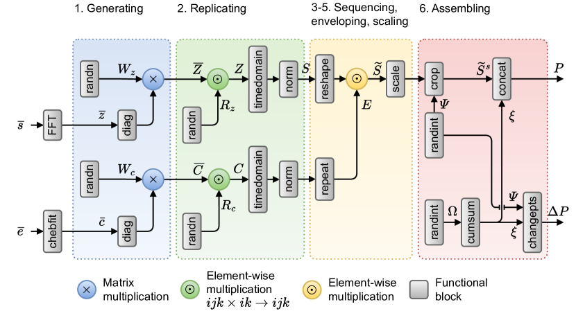
In Fig. 7 we give a diagrammatic representation of the HiFAKES’s architecture. The pseudo-code for the algorithm is listed in Algorithm 3.
In the following subsection, we present the theoretical framework of the proposed generative model.
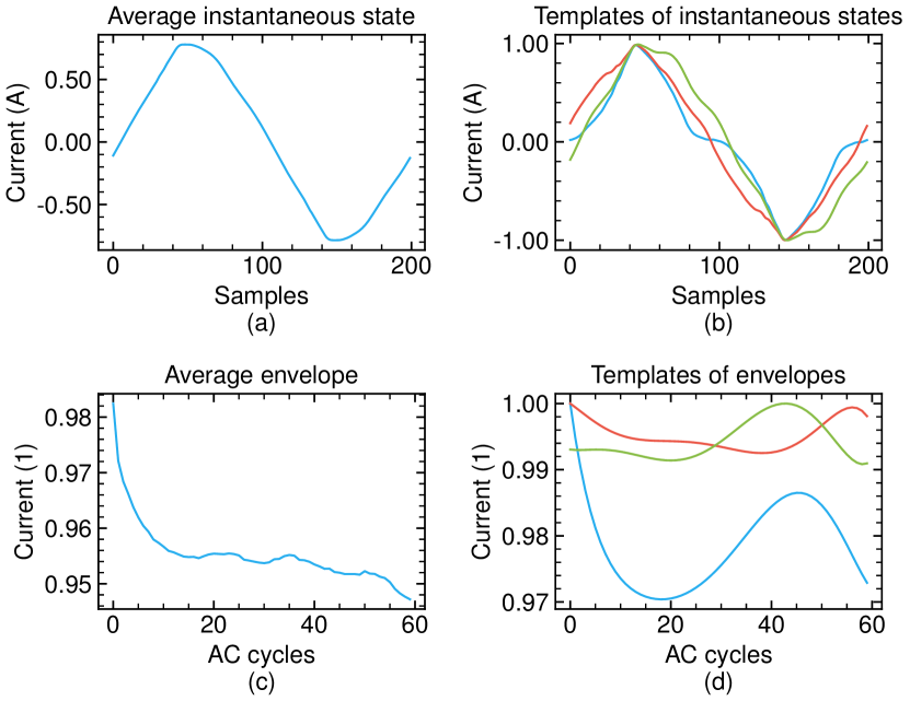
4.2.2 Generating templates for instantaneous states and amplitude envelopes
HiFAKES requires only a single real-world appliance regime signature as a reference to generate a synthetic dataset. In particular, it requires its instantaneous state and amplitude envelope. Depending on the availability of data, these two components can be selected randomly or computed as an average over the given dataset. To cover the variability of signatures in the real-world dataset (), we recommend calculating the average instantaneous state () and the average amplitude envelope ().
Direct computation of these components can be challenging due to several factors: First, frequency fluctuations, i.e., AC cycles have different durations; second, signatures may have varying durations; and third, there may be non-zero mutual phases between any two voltage signals. To address these challenges, we suggest using a frequency-invariant transformation of periodic signals (FITPS) [33]. This transform requires both voltage and current signatures of length and converts them from vectors to matrices, where one dimension corresponds to the number of AC cycles () and the other to the number of samples () within each cycle, i.e., :
| (1) |
where is a set of converted electrical current signatures, where each signature is matrix, and and are voltage and current signatures, respectively. We note that the number should be the same for all signatures. That is, signatures which number of cycles is more than should be split accordingly. Additionally, we normalized all signatures in to the interval. Then, the average instantaneous state () can be computed as:
| (2) |
where is the number of signatures. The amplitude envelope () can be computed as the maximum absolute value of each AC cycle:
| (3) |
Alternatively, both and can be computed from the average signature instead of from the dataset .
The first two steps of the HiFAKES algorithm are performed in the transformed domain to simplify mathematical operations. We apply the fast Fourier transform (FFT) to obtain the spectrum of the reference instantaneous state, denoted as :
| (4) |
Here, is the number of harmonics including the offset. The amplitude envelope can be represented by a polynomial expansion using Chebyshev approximation theorem:
| (5) |
where is the number of Chebyshev polynomials, denotes the Chebyshev coefficients, is the Chebyshev polynomial of order evaluated at a point , and the matrix is pseudo Vandermond matrix. Thus, the transformed domain for the amplitude envelope will be the domain of Chebyshev coefficients. The coefficients can be computed as a solution to the least-squares problem:
| (6) |
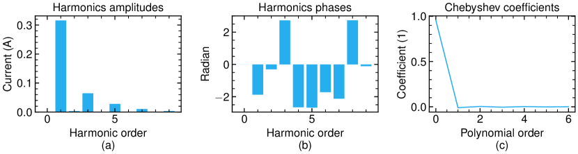
Examples of amplitudes and phases computed from are shown in Fig. 8(a-b), along with the corresponding Chebyshev coefficients in Fig. 8(c).
After computing , it is projected in random directions to generate templates for instantaneous states () (see Fig. 9(a-b) for a visual example):
| (7) |
Here, is a random projection matrix, where represents the number of unique instantaneous states and denotes the number of harmonics. The elements of are complex numbers () with and , where and are the half-normal and normal distributions, respectively. The parameters and represent the location, while and denote the scale of the distributions. Analogously, the templates for amplitude envelopes () can be computed (see Fig. 9(c-d)):
| (8) |
Here, is a random projection matrix. The elements of are defined as , where is the location, and is the scale of the distribution.
The pseudo-code for generating templates for instantaneous states and amplitude envelopes is provided in Algorithm 1.
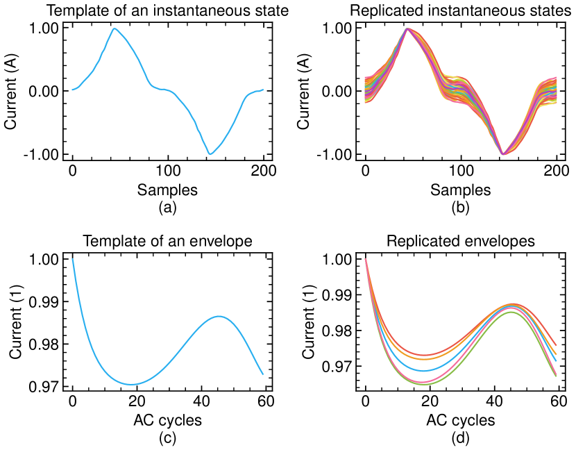
4.2.3 Replicating authentic instantaneous states and amplitude envelopes
Generating a regime signature requires a sequence of enveloped AC cycles, where the cycles and their envelope closely resemble their respective templates. To create such a signature, the instantaneous state template must be replicated according to the number of cycles in the regime. The envelope should then be replicated accordingly. Note that at the replicating stage, we also model the imperfections of the measurement system, which result in several different representations of the actual regime’s signature, as explained in Section 4.1. To account for these variations, we apply multiplicative Gaussian noise to the templates in their respective transformed domains. We recommend vectorizing the computations and obtaining the results in a tensor form (which requires a fixed-size dimension) to efficiently replicate the given templates. For this, we suggest to use the number of cycles () in a program as the size of such dimension so that the total number of replications for instantaneous states is , and for amplitude envelopes, , which is also the number of representations of the actual regime’s signature.
Similarly to step one of HiFAKES’ algorithm, we obtain replicas of instantaneous states as (see Fig. 10(a-b)):
| (9) |
Here, is a random real tensor with elements sampled from the normal distribution . The parameters and control the diversity of the replicated instantaneous states. The indices , , and correspond to the template for the instantaneous state, the replicas, and the harmonics, respectively.
Analogously, replicas of amplitude envelopes can be produced (see Fig. 10(c-d)):
| (10) |
Here, is a random real tensor with elements sampled from the normal distribution . The parameters and control the diversity of the replicated amplitude envelopes. The indices , , and correspond to the template for the amplitude envelope, the replicas, and the Chebyshev polynomial, respectively. In both cases, larger values of the ratio result in higher diversity, and vice versa. The geometrical interpretation of the operations in Eqs. (9) and (10) is that the space around each template is populated with replicated signatures.
Before moving to the next step of the algorithm, HiFAKES transforms instantantaneous states and amplitude envelopes back to the time-domain, and , by using inverse fast Fourier transform (IFFT) and the formula from Eq. (5), respectively:
| (11) |
| (12) |
To ensure that the instantaneous states have unit amplitude, as discussed in Section 4.1, we normalize them as follows:
| (13) |
Since amplitude envelopes should be bounded within , we ensure this by scaling their values to the interval :
| (14) |
where and represent the minimum and maximum values of the vector, respectively, and is computed as:
| (15) |
The pseudo-code for this step is listed in Algorithm 2.
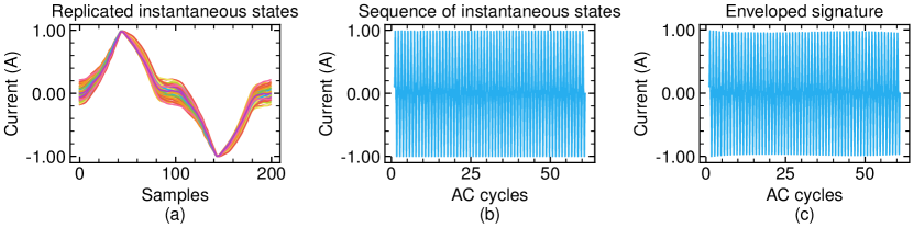
4.2.4 Sequencing, enveloping and scaling
After obtaining the required number of instantaneous states for each regime, the tensor of replicas is reshaped from dimensions to , producing steady-state sequences of cycles for each regime (see Fig. 11(a-b) for illustration).
Since the replicas of amplitude envelopes have a length equal to the number of cycles, , they must be repeated times to match the dimensionality of the instantaneous states in . Specifically, each value of the tensor should be repeated times across the third dimension to obtain a tensor with dimensions :
| (16) |
Thus, the regime signatures () are computed by enveloping the obtained steady-state signatures (see Fig. 11(c)):
| (17) |
Finally, each signature is scaled to simulate real-world regime signatures with varying amplitudes:
| (18) |
Here , where U denotes the uniform distribution, and represent the minimum and maximum amplitudes of the regime, respectively.
4.2.5 Assembling programs
A program, by definition, consists of several regimes. To fit these regimes into a sequence of AC cycles, we introduce a nested set specifying the number of cycles per each regime of each program. E.g., if a program lasts for 50 cycles and consists of three different regimes, then the respective durations of each regime can be 15, 25, 10. Thus, an element of is such that the sum of its elements is , with each subset corresponding to a specific program.
To specify the number of regimes per program, we define the set , which is obtained by sampling integers uniformly from the range , where and represent the minimum and maximum number of regimes in a program, respectively. HiFAKES successively concatenates the number of regimes specified by the variable to generate each program, with each corresponding to a specific program. For example, the signatures of regimes 1 and 2 are concatenated to produce program 1 (see Fig. 12 for illustration), while signatures 3, 4, and 5 are concatenated to form program 2, and so on.
Since each program’s signature has exactly cycles, and the total duration of each regime of a program must be equal to after the concatenation then the regimes durations must be cut off. We cut them according to the values specified in the set multiplied by . Thus, the set of signatures for the program will be:
| (19) |
Here — denotes concatenation across columns of the given matrices i.e., stacking matrices horizontally. denotes -th element of the set , which is unfolded version of the set i.e., elements of are now elements of in the same order as they were in . The function reduces the number of columns of a matrix to .
Finally, HiFAKES computes the change points for the program as:
| (20) |
Here is the cumulative sum set, where the first elements is zero. Change points for all the signatures of -th program are considered as the same.

5 Evaluation
5.1 Reference datasets
To evaluate high-frequency synthetic datasets, we used the following reference datasets: the real-world dataset PLAID, and the synthetic datasets SHED and PIASG. We split the PLAID and the SHED datasets for three subsets containing only: instantaneous states, regimes, and programs. In the Table 1 we collect the statistic on extracted subsets. We filtered all signatures that had at least one AC cycle of 1 ampere to avoid measurement noise. To identify regimes and programs we used the event detector proposed by [34]. PIASG’s subsets for instantaneous states and regimes were generated using the original generative model [16] since it does not support programs generation. We define a regime as a sequence of AC cycles whose amplitude and spectrum does not change more than a predefined threshold. A program is a sequence of AC cycles with at least one of those changes. Using HiFAKES, we generated three corresponding subsets based on the parameters specified in Tables 2 and 3.
| Subset | Dataset name | Number of signatures |
|---|---|---|
| Instantaneous state | PLAID | 32348 |
| PIASG | ||
| SHED | ||
| Regime | PLAID | 582 |
| PIASG | ||
| SHED | ||
| Program | PLAID | 69 |
| SHED |
| Model | |||||||
|---|---|---|---|---|---|---|---|
| Instantaneous state | 99 | 6 | 41 | 789 | 1 | 1, 105 | 1,1 |
| Regime | 291 | 2 | 60 | 1.5, 87 | 1,1 | ||
| Program | 69 | 60 | 16, 53 | 1,2 |
| Model | |||||||||
|---|---|---|---|---|---|---|---|---|---|
|
4.44 | 12.13 | -0.17 | 2.28 | 0.24 | 3.25 | 0.1 | 0.16 | |
| Regime | 2.88 | 1.22 | -0.04 | 0.84 | 0.39 | 1.1 | 0.01 | 0.13 | |
| Program | 0.72 | 7.42 | -0.06 | 2.02 | 1.97 | 4.05 | 0.02 | 0.06 |
5.2 3D metric test (-precision, -recall, authenticity)
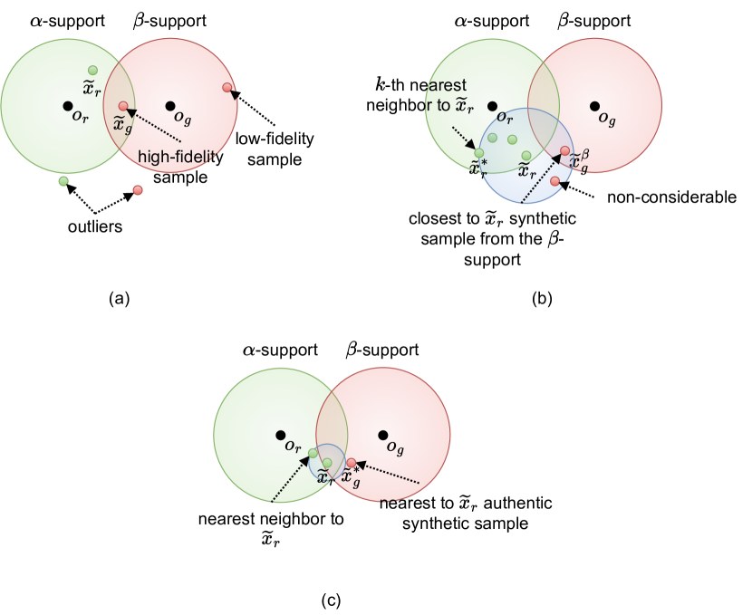
One of the first quantitative metrics named precision and recall for assessing fidelity and diversity of synthetic data with respect to the real data was proposed in [31]. Precision measures how much of the generative distribution can be generated by a part of the real distribution , while recall measures the reverse. In a later work [29], these metrics were generalized to -precision, , and -recall, , which enable inspecting density level sets of real and generative distributions. Additionally, the same work proposed the metric authenticity () to quantify the generalization criteria, thus resulting in a 3D-metric , with higher values indicating better performance.
To compute the -precision and -recall , one should first project the real dataset and the synthetic dataset onto minimum-volume hyper-spheres and , with centers and , respectively. By taking and quantiles of the radii of the mentioned spheres, the estimates of - and -supports can be introduced. Thus, the -support is a concentric Euclidean ball with radius , where is a function that computes the quantile, and is the projection of . The -support is defined in the same fashion i.e., . It is assumed that data points outside of the - or -support are outliers.
Here, we follow the approach given in [35] to project and onto hyper-spheres via feed-forward neural network by minimizing the objective function over the parameters of :
| (21) |
In Table 4 we list all the parameters used for the neural network based on the subset it was trained on. Hence, the -precision is defined as a probability that a synthetic sample resides in the -support:
| (22) |
where is the function that indicates 1 if the condition in the parentheses is true, and 0 otherwise, is the Euclidean distance, and the summation is done over all , and .
| Subsets | # PC |
|
|
Epochs |
|
|||||||
|---|---|---|---|---|---|---|---|---|---|---|---|---|
| Instantaneous state | 2 | {1.18, 1.01} | 2 | 64 | 150 | 4.39 | ||||||
| Regime | {2.34, -5.86} | 64 | 200 | 2.89 | ||||||||
| Program | {6.21, -7.84} | 32 | 200 | 11.47 |
The -recall is defined as a probability that each real sample is locally covered by the nearest synthetic sample from the -support:
| (23) |
where is a synthetic sample belonging to the -support, which is nearest to a real sample . is a Euclidean ball centered at the real sample with a radius equal to the distance to its -th nearest neighbor . The summation is done over all , and .
The authenticity is defined as:
| (24) |
where is the nearest synthetic sample to a real sample , and is the nearest real sample to , and summation is done over all , and .
It is recommended to use integrated metrics -precision and -recall to assess the performance of a generative model in a single number [31] :
| (25) |
where , and . The ideal situation occurs when the real and generative distributions are equal, corresponding to . For a better understanding of the logic behind equations 22, 23 and 24, we provide illustrations for each formula in Fig. 14, respectively. For further details, one can refer to the original paper [29].
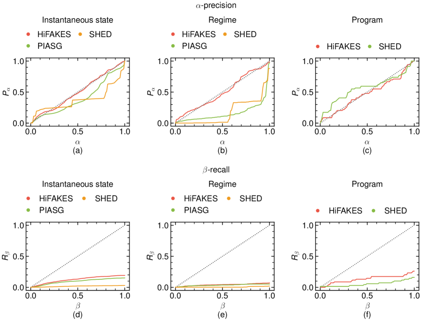
To evaluate the effectiveness of the HiFAKES generative model, we first simulated three subsets of signatures: instantaneous states, regimes, and programs. We then computed 3D metrics for each subset, along with precision () and recall (). To compare the HiFAKES-generated data with reference datasets, we also calculated these metrics for each subset of the reference datasets. The results of our evaluation are summarized in Table 5 and in Fig. 15. Dashed lines in Figs. 15 indicate the ideal scenario.
| Subset | Dataset name | |||||
|---|---|---|---|---|---|---|
| Instantaneous state | HiFAKES | 1.0 | 0.191 | 0.966 | 0.241 | 0.795 |
| PIASG | 0.999 | 0.151 | 0.803 | 0.182 | 0.828 | |
| SHED | 1.0 | 0.03 | 0.686 | 0.025 | 0.935 | |
| Regime | HiFAKES | 0.983 | 0.07 | 0.94 | 0.073 | 0.905 |
| PIASG | 0.973 | 0.052 | 0.32 | 0.06 | 0.933 | |
| SHED | 0.881 | 0.019 | 0.342 | 0 | 0.974 | |
| Program | HiFAKES | 1.0 | 0.261 | 0.929 | 0.26 | 0.681 |
| SHED | 1.0 | 0.159 | 0.806 | 0.104 | 0.884 |
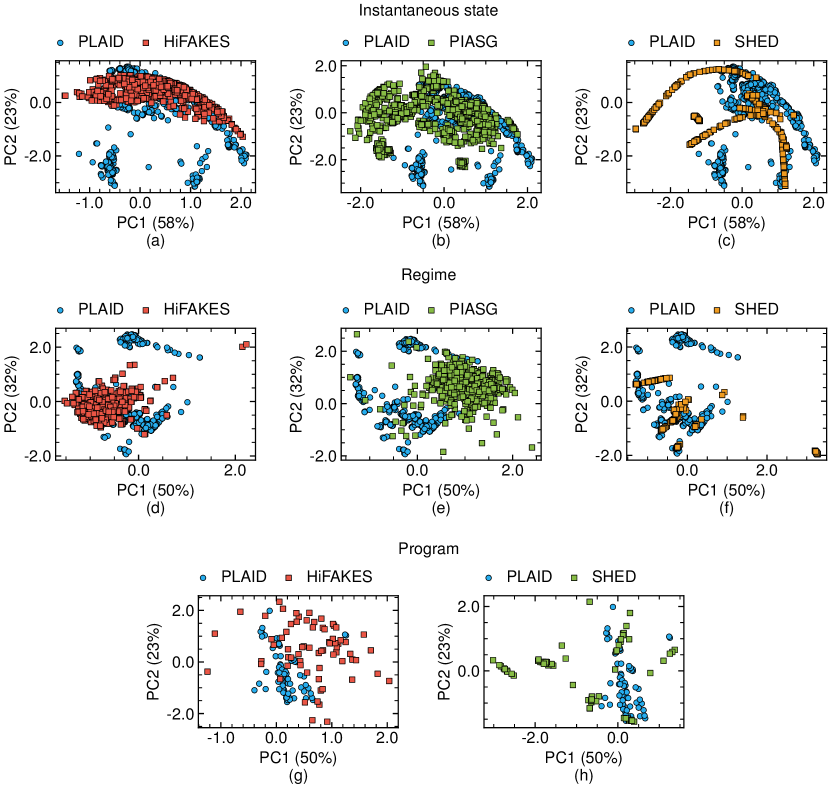
5.3 Domain classifier test
This method involves training a binary classification model to differentiate between real and synthetic signatures [32]. The performance of the model is assessed using the area under the receiver operating characteristic curve (AUC-ROC). An AUC-ROC score of 50% indicates that the model is unable to confidently distinguish between real and synthetic samples, which implies that the synthetic data is of high quality. In contrast, an AUC-ROC score of 100% indicates that the model can perfectly differentiate between real and synthetic signatures, suggesting that the synthetic data is of poor quality.
The domain classifier test was conducted for instantaneous states, regimes, and programs. Each experiment involved obtaining a dataset as a mixture of real and synthetic signatures, computing features, and training and evaluating the classifier. Real signatures were labeled as true positives, while synthetic signatures were labeled as true negatives. The dataset was then split into training and test sets with a 50/50 ratio. Principal components and spherical embeddings were used as features. Two classification models were trained and evaluated using AUC-ROC: linear support vector machines (linear SVM), and the XGBoost implementation of a gradient boosting classifier. The results are summarized in Table 6.
| Subset | Dataset name | AUC-ROC |
| Linear SVM | ||
| Instantaneous state | HiFAKES | 0.51 |
| PIASG | 0.52 | |
| SHED | 0.63 | |
| Regime | HiFAKES | 0.5 |
| PIASG | 0.5 | |
| SHED | 0.5 | |
| Program | HiFAKES | 0.5 |
| SHED | 0.5 | |
| XGBoost | ||
| Instantaneous state | HiFAKES | 0.82 |
| PIASG | 0.85 | |
| SHED | 0.96 | |
| Regime | HiFAKES | 0.86 |
| PIASG | 0.91 | |
| SHED | 0.96 | |
| Program | HiFAKES | 0.66 |
| SHED | 0.8 | |
6 Discussion and concluding remarks
In this work, we introduced HiFAKES, a physics-informed, one-shot generative model that achieves state-of-the-art fidelity, diversity, and generalization. HiFAKES leverages physical principles to enable one-shot data generation while independently controlling each criterion. The model can generate both known and novel appliances from a single electrical current signature or an ”average appliance,” as discussed in Section 4.
Before designing HiFAKES, we analyzed the real-world high-frequency dataset PLAID, and discovered that appliance signatures typically form convex clusters, with each cluster corresponding to a specific state or regime. We hypothesized that the convexity of these clusters results from measurement errors. This insight informed the design of the second stage of the HiFAKES generative model, which focuses on template replication.
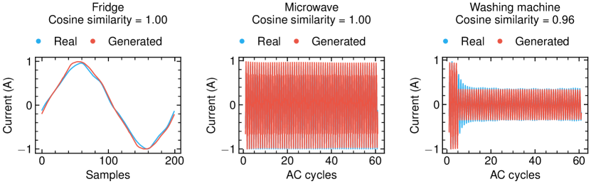
For the first time in the NILM domain, we conducted domain-agnostic tests to evaluate the quality of synthetic datasets: the 3D metric test and the domain classifier test. The 3D metric test demonstrates that HiFAKES significantly outperforms existing generative models in fidelity (with 2.76 times higher -precision) and diversity (with 2.5 times higher -recall). However, HiFAKES faces challenges in generalization, with 10% lower authenticity, meaning it produces signatures that closely resemble existing ones. While this could be a concern for training-dependent models like SynD, it is less problematic for HiFAKES, a training-free, one-shot generative model. In this context, the high -precision combined with lower authenticity metrics underscores the accuracy of the physical principles embedded in HiFAKES, enabling it to generate both known (as shown in Fig. 16) and unseen (as illustrated in Fig. 13 (a,d,g)) appliances from a single example.
It is important to note that the signatures shown in Fig. 16 were not deliberately generated to match the given appliances. Rather, these signatures resulted from random projections of the average instances provided for each subset (instantaneous state, regime, and program). We identified the signatures that closely resemble real ones using a similarity search with the cosine metric. This phenomenon can be explained by examining the first stage of the HiFAKES algorithm, which controls both fidelity and generalization. Fidelity is determined by the provided training example, i.e., the signature, while generalization is influenced by the distribution of values in the projection matrix . Although we recommended sampling these values from half-normal and normal distributions with adjustable parameters, other types of distributions, such as conditional distributions, could also be employed depending on the understanding of the projection mechanics. The question of how to explicitly control generalization through custom distribution design remains open for further investigation.
In the domain classifier test, HiFAKES performs nearly optimally, comparable to SHED and PIASG across all subsets when using a linear classifier. However, when employing a more powerful model like XGBoost, a gradient boosting model, HiFAKES signatures are significantly harder to identify as synthetic compared to other generative models. Notably, the appliance programs generated by HiFAKES are almost indistinguishable from real ones, with the AUC-ROC score only 16% higher than the optimal value.
Given HiFAKES lower generalization ability compared to its predecessors, it may not be the best choice for privacy-sensitive tasks, such as sharing a dataset copy while protecting the original signatures. The risk that HiFAKES might generate synthetic data too similar to the original could raise privacy concerns. In these cases, models like PIASG and SHED, which generate more novel signatures, would be more effective in preserving privacy. These models are better suited for ensuring that shared datasets do not unintentionally reveal sensitive information, making them a safer option for privacy-focused applications.
The signatures generated by HiFAKES can effectively simulate power consumption for simultaneously operating appliances, which is valuable for training NILM models. This can be done by creating linear combinations of the generated signatures using binary coefficients, as each signature already includes its own amplitude. Specifically, a binary matrix with dimensions can be generated, where represents the number of training signatures and indicates the number of appliances operating simultaneously. By multiplying this matrix by the HiFAKES-generated signatures matrix , the desired dataset () can be produced:
| (26) |
This method works because of Kirchoff’s law and the fact that all the generated signatures are assumed to be synchronous with their respective voltage.
The HiFAKES generative model is implemented entirely in Python and is available via the provided link. All experiments were conducted on a personal laptop with an M2 processor and 8GB of RAM. Given hardware, generating 1,000 programs for 20 appliances (50 signatures per appliance), each with a duration of 10 seconds, takes approximately 17 seconds.
CRediT author statement
Ilia Kamyshev Conceptualization, Methodology, Software, Formal analysis, Investigation, Writing - Original Draft, Visualization, Writing - Editing. Sahar Moghimian Hoosh Methodology, Formal analysis, Investigation, Writing - Original Draft, Writing - Review & Editing. Henni Ouerdane: Resources, Writing - Review & Editing, Supervision.
Acknowledgements
The authors acknowledge partial support by the Skoltech program: Skolkovo Institute of Science and Technology – Hamad Bin Khalifa University Joint Projects.
References
- [1] H. Youssef, S. Kamel, M. H. Hassan, L. Nasrat, Optimizing energy consumption patterns of smart home using a developed elite evolutionary strategy artificial ecosystem optimization algorithm, Energy 278 (2023) 127793.
- [2] S. Dai, F. Meng, Q. Wang, X. Chen, Federatednilm: A distributed and privacy-preserving framework for non-intrusive load monitoring based on federated deep learning, in: 2023 International Joint Conference on Neural Networks (IJCNN), IEEE, 2023, pp. 01–08.
- [3] G. Huebner, D. Shipworth, I. Hamilton, Z. Chalabi, T. Oreszczyn, Understanding electricity consumption: A comparative contribution of building factors, socio-demographics, appliances, behaviours and attitudes, Applied energy 177 (2016) 692–702.
- [4] Á. Hernández, A. Ruano, J. Ureña, M. Ruano, J. Garcia, Applications of nilm techniques to energy management and assisted living, IFAC-PapersOnLine 52 (11) (2019) 164–171.
- [5] K.-K. Kee, Y. S. Lim, J. Wong, K. H. Chua, Non-intrusive load monitoring (nilm)–a recent review with cloud computing, in: 2019 IEEE International Conference on Smart Instrumentation, Measurement and Application (ICSIMA), IEEE, 2019, pp. 1–6.
- [6] G. W. Hart, Nonintrusive appliance load monitoring, Proceedings of the IEEE 80 (12) (1992) 1870–1891.
- [7] D. Li, J. Li, X. Zeng, V. Stankovic, L. Stankovic, C. Xiao, Q. Shi, Transfer learning for multi-objective non-intrusive load monitoring in smart building, Applied Energy 329 (2023) 120223.
- [8] M. Kaselimi, E. Protopapadakis, A. Voulodimos, N. Doulamis, A. Doulamis, Towards trustworthy energy disaggregation: A review of challenges, methods, and perspectives for non-intrusive load monitoring, Sensors 22 (15) (2022) 5872.
- [9] C. Klemenjak, A. Reinhardt, L. Pereira, S. Makonin, M. Bergés, W. Elmenreich, Electricity consumption data sets: Pitfalls and opportunities, in: Proceedings of the 6th ACM international conference on systems for energy-efficient buildings, cities, and transportation, 2019, pp. 159–162.
- [10] X. Wu, D. Jiao, L. You, Nonintrusive on-site load-monitoring method with self-adaption, International Journal of Electrical Power & Energy Systems 119 (2020) 105934.
- [11] D. R. Chavan, D. S. More, A. M. Khot, Iedl: Indian energy dataset with low frequency for nilm, Energy Reports 8 (2022) 701–709.
- [12] D. Chen, D. Irwin, P. Shenoy, Smartsim: A device-accurate smart home simulator for energy analytics, in: 2016 IEEE International Conference on Smart Grid Communications (SmartGridComm), IEEE, 2016, pp. 686–692.
- [13] N. Buneeva, A. Reinhardt, Ambal: Realistic load signature generation for load disaggregation performance evaluation, in: 2017 ieee international conference on smart grid communications (smartgridcomm), IEEE, 2017, pp. 443–448.
- [14] S. Henriet, U. Şimşekli, B. Fuentes, G. Richard, A generative model for non-intrusive load monitoring in commercial buildings, Energy and Buildings 177 (2018) 268–278.
- [15] C. Klemenjak, C. Kovatsch, M. Herold, W. Elmenreich, A synthetic energy dataset for non-intrusive load monitoring in households, Scientific data 7 (1) (2020) 108.
- [16] I. Kamyshev, S. M. Hoosh, H. Ouerdane, Physics-informed appliance signatures generator for energy disaggregation, in: 2023 IEEE 7th Conference on Energy Internet and Energy System Integration (EI2), IEEE, 2023, pp. 3591–3596.
- [17] H. K. Iqbal, F. H. Malik, A. Muhammad, M. A. Qureshi, M. N. Abbasi, A. R. Chishti, A critical review of state-of-the-art non-intrusive load monitoring datasets, Electric Power Systems Research 192 (2021) 106921.
- [18] P. A. Schirmer, I. Mporas, Non-intrusive load monitoring: A review, IEEE Transactions on Smart Grid 14 (1) (2022) 769–784.
- [19] T. Kriechbaumer, H.-A. Jacobsen, Blond, a building-level office environment dataset of typical electrical appliances, Scientific data 5 (1) (2018) 1–14.
- [20] M. Kahl, A. U. Haq, T. Kriechbaumer, H.-A. Jacobsen, Whited-a worldwide household and industry transient energy data set, in: 3rd international workshop on non-intrusive load monitoring, 2016, pp. 1–4.
- [21] T. Picon, M. N. Meziane, P. Ravier, G. Lamarque, C. Novello, J.-C. L. Bunetel, Y. Raingeaud, Cooll: Controlled on/off loads library, a public dataset of high-sampled electrical signals for appliance identification, arXiv preprint arXiv:1611.05803 (2016).
- [22] J. Gao, S. Giri, E. C. Kara, M. Bergés, Plaid: a public dataset of high-resoultion electrical appliance measurements for load identification research: demo abstract, in: proceedings of the 1st ACM Conference on Embedded Systems for Energy-Efficient Buildings, 2014, pp. 198–199.
- [23] K. Anderson, A. Ocneanu, D. Benitez, D. Carlson, A. Rowe, M. Berges, Blued: A fully labeled public dataset for event-based non-intrusive load monitoring research, in: Proceedings of the 2nd KDD workshop on data mining applications in sustainability (SustKDD), Vol. 7, ACM New York, 2012, pp. 1–5.
- [24] A. M. Tartakovsky, C. O. Marrero, P. Perdikaris, G. D. Tartakovsky, D. Barajas-Solano, Physics-informed deep neural networks for learning parameters and constitutive relationships in subsurface flow problems, Water Resources Research 56 (5) (2020) e2019WR026731.
- [25] J. Willard, X. Jia, S. Xu, M. Steinbach, V. Kumar, Integrating scientific knowledge with machine learning for engineering and environmental systems, ACM Computing Surveys 55 (4) (2022) 1–37.
- [26] C. Beckel, W. Kleiminger, R. Cicchetti, T. Staake, S. Santini, The eco data set and the performance of non-intrusive load monitoring algorithms, in: Proceedings of the 1st ACM conference on embedded systems for energy-efficient buildings, 2014, pp. 80–89.
- [27] A. Reinhardt, P. Baumann, D. Burgstahler, M. Hollick, H. Chonov, M. Werner, R. Steinmetz, On the accuracy of appliance identification based on distributed load metering data, in: 2012 Sustainable Internet and ICT for Sustainability (SustainIT), IEEE, 2012, pp. 1–9.
- [28] S. Barker, A. Mishra, D. Irwin, E. Cecchet, P. Shenoy, J. Albrecht, et al., Smart*: An open data set and tools for enabling research in sustainable homes, SustKDD, August 111 (112) (2012) 108.
- [29] A. Alaa, B. Van Breugel, E. S. Saveliev, M. van der Schaar, How faithful is your synthetic data? sample-level metrics for evaluating and auditing generative models, in: International Conference on Machine Learning, PMLR, 2022, pp. 290–306.
- [30] P. Eigenschink, T. Reutterer, S. Vamosi, R. Vamosi, C. Sun, K. Kalcher, Deep generative models for synthetic data: A survey, IEEE Access 11 (2023) 47304–47320.
- [31] P. Flach, M. Kull, Precision-recall-gain curves: Pr analysis done right, Advances in neural information processing systems 28 (2015).
- [32] I. E. Livieris, N. Alimpertis, G. Domalis, D. Tsakalidis, An evaluation framework for synthetic data generation models, in: IFIP International Conference on Artificial Intelligence Applications and Innovations, Springer, 2024, pp. 320–335.
- [33] P. Held, S. Mauch, A. Saleh, D. O. Abdeslam, D. Benyoucef, Frequency invariant transformation of periodic signals (fit-ps) for classification in nilm, IEEE Transactions on Smart Grid 10 (5) (2018) 5556–5563.
- [34] B. Völker, M. Pfeifer, P. M. Scholl, B. Becker, Annoticity: A smart annotation tool and data browser for electricity datasets, in: Proceedings of the 5th International Workshop on Non-Intrusive Load Monitoring, 2020, pp. 1–5.
- [35] L. Ruff, R. Vandermeulen, N. Goernitz, L. Deecke, S. A. Siddiqui, A. Binder, E. Müller, M. Kloft, Deep one-class classification, in: International conference on machine learning, PMLR, 2018, pp. 4393–4402.