SORSA: Singular Values and Orthonormal Regularized Singular Vectors Adaptation of Large Language Models

Abstract

The rapid advancement in large language models (LLMs) comes with a significant increase in their parameter size, presenting challenges for adaptation and fine-tuning. Parameter-efficient fine-tuning (PEFT) methods are widely used to adapt LLMs for downstream tasks efficiently. In this paper, we propose Singular Values and Orthonormal Regularized Singular Vectors Adaptation, or SORSA, a novel PEFT method. We introduce a method to analyze the variation of the parameters by performing singular value decomposition (SVD) and discuss and analyze SORSA’s superiority in minimizing the alteration in the SVD aspect. Each SORSA adapter consists of two main parts: trainable principal singular weights $W_{p}=U_{p}\text{diag}(S_{p})V^{\top}_{p}$, and frozen residual weights $W_{r}=U_{r}\text{diag}(S_{r})V^{\top}_{r}$. These parts are initialized by performing SVD on pre-trained weights. Moreover, we implement and analyze an orthonormal regularizer, which we prove could decrease the condition number of $W_{p}$ and allows the optimization to be more efficient. SORSA adapters could be merged during inference, thus eliminating any inference latency. After all, SORSA shows a faster convergence than PiSSA and LoRA in our experiments. On the GSM-8K benchmark, Llama 2 7B adapted using SORSA achieved 56.03% accuracy, surpassing LoRA (42.30%), Full FT (49.05%), and PiSSA (53.07%). On the MATH benchmark, SORSA achieved 10.36% accuracy, outperforming LoRA (5.50%), Full FT (7.22%), and PiSSA (7.44%). We conclude that SORSA offers a new perspective on parameter-efficient fine-tuning, demonstrating remarkable performance. The code is available at https://github.com/Gunale0926/SORSA.

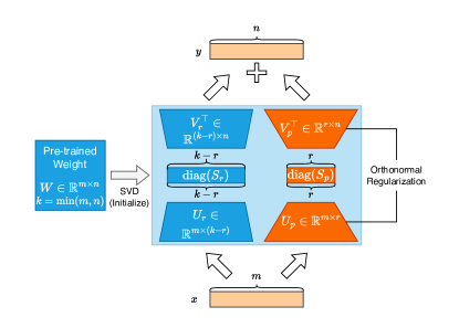
Figure 1: Architecture of a SORSA adapter. We only train parts rendered in orange ($U_{p}$, $\text{diag}(S_{p})$ and $V^{\top}_{p}$), and freeze parts rendered in blue ($U_{r}$, $\text{diag}(S_{r})$ and $V^{\top}_{r}$).

1 Introduction

Pre-trained large language models (LLMs) show remarkable generalization abilities, allowing them to perform various kinds of natural language processing (NLP) tasks (Peng et al., 2024; Touvron et al., 2023; Dubey et al., 2024; Radford et al., 2019; OpenAI, 2023). For specific downstream tasks, full parameter fine-tuning, which continues training all parameters of LLMs on downstream data, is widely used.

However, as the number of parameters in LLMs rapidly increases, full parameter fine-tuning becomes increasingly inefficient. For example, the estimated VRAM requirement for fully fine-tuning Llama 2 7B using Float32 could approach approximately 100 GB, making it unlikely to fully fine-tune the model on a single GPU with current technology. Additionally, the VRAM requirement for fully fine-tuning Llama 2 70B using Float32 exceeds 1 TB (Touvron et al., 2023; Anthony et al., 2023), thus rendering it unfeasible on a single GPU with current technology.

To address these challenges, several parameter-efficient fine-tuning (PEFT) methods (Houlsby et al., 2019; Lester et al., 2021; Hu et al., 2021) have been proposed. These methods enable the training of only a limited number of parameters, which significantly reduces VRAM requirements while achieving comparable or even superior performance to full fine-tuning. For instance, tuning Llama 2 7B in Float32 by LoRA (Hu et al., 2021) with a rank of 128 only takes approximately 60GB VRAM, which allows training on 1 $\times$ NVIDIA A100 (80GB), or even 3 $\times$ NVIDIA RTX 4090 (24GB).

Among those PEFT methods, LoRA (Hu et al., 2021) and its variants (Zhang et al., 2023; Meng et al., 2024; Liu et al., 2024; Dettmers et al., 2024) had become increasingly popular due to their: 1. Low training VRAM requirement 2. No inference latency 3. Versatility in different neuron network architectures.

In this paper, we propose a novel PEFT approach, Singular Values and Orthonormal Regularized Singular Vectors Adaptation, or SORSA. A SORSA adapter has two main parts: principal singular weights $W_{p}=U_{p}\text{diag}(S_{p})V^{\top}_{p}$, and residual weights $W_{r}=U_{r}\text{diag}(S_{r})V^{\top}_{r}$. These two parts are initialized by performing singular value decomposition (SVD) on pre-trained weight. Residual singular values and vectors will be merged into one matrix and frozen while training. We only train principal singular values and vectors with an orthonormal regularizer implemented to keep the orthonormality of $U_{p}$ and $V_{p}^{\top}$. The architecture of a SORSA adapter is illustrated in Figure 1.

Furthermore, we analyze the pattern of variation of singular values and vectors during parameter updating and discuss the different patterns of partial fine-tuning (FT), LoRA, SORSA without regularizer, and SORSA with regularizer concerning singular values and vectors’ updating.

We also provide a comprehensive gradient analysis that provides a mathematical foundation for SORSA. This analysis demonstrates several crucial properties of our method, including the convexity of the regularizer, Lipschitz continuity of the gradient, bounds on the hyperparameter $\gamma$. Moreover, we prove that SORSA improves the condition number of the optimization problem compared to unregularized approaches.

SORSA retains all the benefits of LoRA and its variants while demonstrating remarkable performance compared to PiSSA, LoRA, and full parameter fine-tuning in our experiments.

2 Related Works

Parameter-efficient fine-tuning (PEFT) methods have been developed to address the inefficiency of full parameter fine-tuning for large language models. These methods focus on adapting the model for downstream tasks while updating only a few parameters and keeping most of the model’s weights frozen. This approach significantly reduces the memory and computational requirements during training, especially VRAM.

Adapter-based PEFT is the first type of PEFT, which was initially designed by Houlsby et al. (2019). It introduces additional trainable non-linear blocks into the frozen pre-trained model, which could effectively tune the pre-trained model with a limited amount of trainable parameters. Its variants, e.g., Lin et al. (2020), reduce the number of adapter layers per block, and He et al. (2022) focus on adding adapter modules parallel to existing layers. However, all adapter-based PEFT methods introduce inference latency due to their non-mergeable attribute.

Prompt-based PEFT is also a well-known type of PEFT, which was first proposed in Lester et al. (2021). There are several variants of this work, including Liu et al. (2022); Razdaibiedina et al. (2023). However, they have some inevitable shortcomings, such as potential performance limitations compared to full parameter fine-tuned models, additional inference latency due to expanding the length of the total input to the model, and the complexity of designing effective initialization.

LoRA (Hu et al., 2021) and its variants are the most popular type of PEFT methods. This type of PEFT is popular for its on-par or better performance than full parameter fine-tuning without introducing any inference latency. LoRA could be represented by equation $W=W_{0}+BA$, where $W_{0}\in\mathbb{R}^{m\times n}$ is the pre-trained weight, $A\in\mathbb{R}^{m\times r}$, using Gaussian initialization, and $B\in\mathbb{R}^{r\times n}$, using zero initialization, are low-rank matrices. Its variant, for example, AdaLoRA (Zhang et al., 2023) introduces an SVD decomposition and pruning for least significant singular values for more efficient parameter updating. DoRA (Liu et al., 2024) proposed a novel way to decompose weight into direction and magnitude by $W=\underline{m}\frac{W_{0}+\underline{BA}}{\|W_{0}+\underline{BA}\|_{c}}$, where $\underline{m}$ is initialized by $\underline{m}=\|W_{0}+\underline{BA}\|_{c}$, $\|\cdot\|_{c}$ denotes column-wise norm. The results show that DoRA has a better learning capacity than LoRA. However, DoRA introduced a calculation of norm in every training step, which makes it much more inefficient in training than LoRA. OLoRA (Büyükakyüz, 2024) uses QR decomposition to initialize the LoRA adapters $A$ and $B$, which initializes $B$ as an orthogonal matrix. They discusses the significance of orthonormality in neural networks’ weight (See Section 5 for more details). In their experiments, OLoRA demonstrates faster convergence than LoRA. PiSSA (Meng et al., 2024) decomposes pre-trained weight $W_{0}=U\text{diag}(S)V^{\top}$ by Singular Value Decomposition (SVD), and then splits $W_{0}$ into $W_{pri}$ and $W_{res}$: $W_{pri}=AB$ which is trainable, where $A=U_{[:r]}\text{diag}(S^{\frac{1}{2}}_{[:r]})$ and $B=\text{diag}(S^{\frac{1}{2}}_{[:r]})V^{\top}_{[:r]}$; $W_{res}=U_{[:r,:r]}\text{diag}(S_{[:r]})V^{\top}_{[:r,:]}$ which is frozen. PiSSA results a faster convergence speed and better fitting compared to LoRA. SORSA has a similar architecture to PiSSA, which both conducts SVD and replaces pre-trained weights with residual singular weights. SORSA inherits LoRA and its variants’ benefits, including low training VRAM requirement, no inference burden, and versatility in different architectures.

Other methods. There are also a few efficient adapting methods with unique techniques. For example, GaLore (Zhao et al., 2024) is a memory-efficient PEFT method that reduces VRAM usage by leveraging gradient accumulation and low-rank approximation. Despite its efficiency, GaLore’s complex implementation, involving perform SVD on gradients, adds computational complexity and may face scalability issues for very large models. LISA (Pan et al., 2024) uses a layer-wise importance sampling approach, prioritizing layers that significantly impact model performance, and selectively fine-tune essential parameters.

3 Singular Values and Vectors Analysis

3.1 Singular Value Decomposition

The geometric meaning of SVD can be summarized as follows: for every linear mapping $W:K^{m}\to K^{n}$, the singular value decomposition finds a set of orthonormal bases in both the original space and the image space such that $W$ maps the $i$-th basis vector of $K^{m}$ to a non-negative multiple of the $i$-th basis vector of $K^{n}$, and maps the remaining basis vectors of $K^{m}$ to the zero vector. In other words, the matrix $W$ can be represented as $\Sigma$ on these selected bases, where $\Sigma$ is a diagonal matrix with all non-negative diagonal elements.

According to the meaning of SVD, giving a matrix $W\in\mathbb{R}^{m\times n}$, let $k=\min(m,n)$, we could perform SVD to decompose $W$ by $W=U\text{diag}(S)V^{\top}$. Here, $U\in\mathbb{R}^{m\times k}$ is matrix of left singular vectors and have orthonormal columns, $V\in\mathbb{R}^{n\times k}$ is matrix of right singular vectors and have orthonormal columns, and $S\in\mathbb{R}^{k}$ are singular values $\sigma^{1},\sigma^{2}\ldots\sigma^{k}$ arranged in descending order. $\text{diag}(W)$ denotes a function to form a diagonal matrix from $W$.

3.2 Analysis Method

The study of DoRA (Liu et al., 2024) introduces an analysis method that focuses on the deviation of magnitude and direction ($\Delta M,\Delta D$) during training of full parameter fine-tuning and LoRA (Hu et al., 2021). They discovered that the distinction between full parameter fine-tuning and LoRA likely affects their learning ability difference. Inspired by their methods, we propose a novel method that analyzes the correlation between the deviation of singular values ($\Delta\Sigma$) and singular vectors ($\Delta D$) from pre-trained matrices during updating. Our analysis suggests a significant difference in singular values and vectors’ stability and an updating pattern of partial fine-tuning, LoRA, and SORSA.

The singular value and vector variations between pre-trained weight $W_{0}\in\mathbb{R}^{m\times n}$ and tuned weight $W_{t}\in\mathbb{R}^{m\times n}$, which $t$ denotes the training step, could be defined as follows:

$$\Delta\Sigma_{t}=\frac{\Sigma_{i=1}^{k}\left|\sigma_{t}^{i}-\sigma_{0}^{i}\right|}{k}$$ (1)

Here, $\Delta\Sigma_{t}$ represents singular value variants between $W_{0}$ and $W_{t}$ at training step $t$. $\sigma^{i}_{t}$ denotes the $i$-th element in diagonal of $\Sigma_{t}$, where $\Sigma_{t}$ is decomposed from $W_{t}$ by performing SVD, $k=\min(m,n)$;

$$\Delta U_{t,j}=\left|\langle{\mathbf{u}}_{t}^{j},{\mathbf{u}}_{0}^{j}\rangle\right|$$ (2)

$$\Delta V^{\top}_{t,i}=\left|\langle{\mathbf{v}}_{t}^{i},{\mathbf{v}}_{0}^{i}\rangle\right|$$ (3)

$$\Delta D_{t}=1-\frac{1}{2k}\sum_{i=0}^{k}(\Delta U_{t,i}+\Delta V^{\top}_{t,i})$$ (4)

Here, $k=\min(m,n)$; ${\mathbf{u}}_{t}^{j}$ denotes the $j$-th column vector of matrix $U_{t}$, and ${\mathbf{v}}_{t}^{i}$ denotes the $i$-th row vector of matrix $V_{t}^{\top}$; $\Delta D_{t}\in(0,1)$ represents variation of singular vectors between $W_{0}$ and $W_{t}$ at training step $t$; $U_{t}$ and $V_{t}^{\top}$ are decomposed from $W_{t}$ by performing SVD.

We adopt the analysis on Llama 2 7B (Touvron et al., 2023) using the first 100K data of MetaMathQA (Yu et al., 2024). We test partial fine-tuning, LoRA, and SORSA (with regularizer and without regularizer). See Section B.1 for training details of the analysis.

3.3 Analysis Result

This section analyzes the results of different training methods: partial fine-tuning, LoRA, and SORSA based on the data we collect. The analysis data is illustrated in Figure 2.

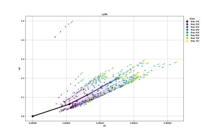
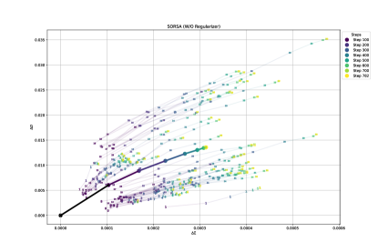
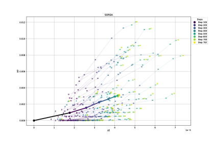
Figure 2: $\Delta D$ and $\Delta\Sigma$ of each trainable parameters during training steps. Numbers in the plot represent layer of the weight. Dots represent mean $\Delta D$ and $\Delta\Sigma$ at specific step.

The partial fine-tuning and LoRA methods analysis show that both methods exhibit significant adjustments in significant vectors $\Delta D$. This substantial alteration disrupts the characteristics of the pre-trained matrix and is likely to affect the model’s generalization ability. Moreover, the updates of all parameters in both partial fine-tuning and LoRA methods show a parallel updating pattern across weights in different layers, which emphasizes a restriction of these methods and may lead to a potentially disruptive modification of the generalization ability.

SORSA with regularizer shows $\Delta D$ and $\Delta\Sigma$ are in a much smaller range than other analysis methods. Moreover, different matrices demonstrated unrelated updating patterns, compared to all parallel-like other three methods, indicating that the updates in the SORSA are less constrained and potentially converge faster. In contrast, SORSA without the orthonormal regularizer exhibits a greater $\Delta D$ and $\Delta\Sigma$ alteration at each training step compared to SORSA with the regularizer. SORSA without regularizer also shows a linear-like updating pattern, similar to LoRA and partial FT. The result verifies the importance of regularizer in maintaining stability and minimizing the deviation from pre-trained matrices during the training process. These updating patterns indicate that SORSA maintains the characteristics of the pre-trained matrix better, thus potentially preserving the model’s generalization ability more effectively. This property allows SORSA adapters to be trained with higher learning rates without showing noticeable over-fitting compared to other tuning methods.

4 SORSA: Singular Value and Orthonormal Regularized Singular Vector Adaptation

According to the definition of SVD in Section 3.1, given a rank $r$ where $r\ll k$, we could perform the low-rank approximation by selecting the first $r$ items on the diagonal of $\Sigma$, which is the first $r$ most significant singular values, and also select the first $r$ columns of $U$ and first $r$ rows of $V^{\top}$, which correspond to the selected singular values. By performing SVD low-rank approximation, we could get a low-rank matrix that preserves the largest significant values and vectors, containing the matrix’s most significant data.

Therefore, for a pre-trained weight $W_{0}\in\mathbb{R}^{m\times n}$, we could split it based on its singular value into principal weight $W_{p}$ and residual weight $W_{r}$, where $W_{p}$ contains the most important part of information of the matrix, and $W_{r}$ contains the least significant part:

$$W_{p}=U_{[:,:r]}\text{diag}(S_{[:r]})V^{\top}_{[:r,:]}\in\mathbb{R}^{m\times n}$$ (5)

$$W_{r}=U_{[:,r:]}\text{diag}(S_{[r:]})V^{\top}_{[r:,:]}\in\mathbb{R}^{m\times n}$$ (6)

Here, $U$ represents the matrix of left singular vectors, $S$ represents the singular values, $\text{diag}(W)$ denotes a function to form a diagonal matrix from $W$, and $V$ represents the matrix of right singular vectors. We use PyTorch (Paszke et al., 2019) syntax to demonstrate matrix selection, where $[:,:r]$ denotes selecting the first $r$ columns of the matrix, and $[r:,:]$ denotes selecting the last $r$ rows of the matrix. We rewrite $U_{[:,:r]}$, $S_{[:r]}$ and $V^{\top}_{[:r,:]}$, which consist $W_{p}$ as $U_{p}$, $S_{p}$ and $V^{\top}_{p}$ for simplicity, and rewrite $U_{[:,r:]}$, $S_{[:r]}$ and $V^{\top}_{[r:,:]}$, which consist $W_{r}$ as $U_{r}$, $S_{r}$ and $V^{\top}_{r}$ correspondingly.

The initialization of $W_{r}$ in SORSA is the same as PiSSA (Meng et al., 2024). Nevertheless, unlike PiSSA which merge $\text{diag}(S_{p})$ with $U_{p}$ and $V^{\top}_{p}$ into $A$ and $B$ by $A=U_{p}\text{diag}(S_{p})^{\frac{1}{2}}$ and $B=\text{diag}(S_{p})^{\frac{1}{2}}V^{\top}_{p}$, SORSA remains $U_{p}$, $S_{p}$, and $V^{\top}_{p}$ in separate matrices. SORSA is defined by Equation 7, which is initially equivalent to the pre-trained weight $W_{0}$.

During training, $W_{r}$ remains frozen, and only $U_{p}$, $S_{p}$, and $V^{\top}_{p}$ are updated.

SORSA is defined as:

$$\text{SORSA}(x):=x(W_{r}+W_{p})=xW_{r}+xU_{p}\text{diag}(S_{p})V^{\top}_{p}$$ (7)

In our implementation, we use a optimized version of SORSA equation which results a much faster computation speed, and could approach to the speed of LoRA. See Appendix A for more details.

We adopt an orthonormal regularizer similar to (Zhang et al., 2023) for $U_{p}$ and $V^{\top}_{p}$. We verify its importance and effectiveness in Section 5.

$${\mathcal{L}}_{reg}=\|U^{\top}_{p}U_{p}-I\|_{F}+\|V^{\top}_{p}V_{p}-I\|_{F}$$ (8)

Where ${\mathcal{L}}_{reg}$ is the orthonormal regularizer loss, the $U_{p}$ and $V^{\top}_{p}$ are each orthonormal vectors in columns and rows, respectively, after initialization due to SVD’s property. The regularizer could keep their orthonormality during training.

Therefore, parameter updating of $W_{p}$ in a SORSA adapter at training step $t$ could be expressed as:

$$W_{p,t+1}= W_{p,t}-\eta_{t}\nabla_{W_{p,t}}{\mathcal{L}}_{train}-\gamma_{t}\nabla_{W_{p,t}}{\mathcal{L}}_{reg}$$ (9)

At training step $t$, $\nabla_{W_{p,t}}{\mathcal{L}}_{train}$ denotes the gradient of ${\mathcal{L}}_{train}$ respect to $W_{p,t}$, and $\nabla_{W_{p,t}}{\mathcal{L}}_{reg}$ denotes the gradient of ${\mathcal{L}}_{reg}$ respect to the orthonormal regularizer loss $W_{p,t}$. $\eta_{t}$ and $\gamma_{t}$ are the learning rate for training loss and regularizer loss at step $t$, respectively.

We update the SORSA as Equation 10 for implementation simplicity.

$$W_{p,t+1}= W_{p,t}-\eta_{t}\left(\nabla_{W_{p,t}}{\mathcal{L}}_{train}+\frac{\gamma}{\eta_{d}}\nabla_{W_{p,t}}{\mathcal{L}}_{reg}\right)$$ (10)

$\eta_{d}$ is the maximum learning rate which is given from the scheduler. This implementation allows us to use only one optimizer and scheduler to deal with two different learning rates separately.

5 Gradient Analysis

In this section, we present a comprehensive mathematical analysis of the SORSA method which mainly focus on the effect of orthonormal regularization. Our investigation elucidates the key optimization properties of SORSA, providing a theoretical foundation for its advantages. We explore four critical aspects: the convexity of the regularizer, the Lipschitz continuity of the gradient, bounds on the hyperparameter $\gamma$, and the impact on the condition number of the optimization problem.

The proofs of the theorems and lemmas, along with additional mathematical details, are provided in Appendix C.

Our analysis reveals fundamental theoretical properties of SORSA, establishing its mathematical soundness and demonstrating its optimization advantages. We prove two key theorems that form the cornerstone of our theoretical framework:

Theorem 1.

The regularizer ${\mathcal{L}}_{reg}$ is convex.

Theorem 2.

The gradient of the regularizer ${\mathcal{L}}_{reg}$ is Lipschitz continuous.

These properties collectively ensure a well-behaved optimization landscape, facilitating stable and efficient training of SORSA adapters.

Building upon these foundational results, we further analyze the bounds of the hyperparameter $\gamma$, a critical factor in the performance of SORSA:

Theorem 3.

For convergence of gradient descent, the learning rate $\eta_{d}$ and regularization parameter $\gamma$ must satisfy:

$$0\leq\gamma<\frac{2}{k\eta_{d}}-L_{train}$$ (11)

This theorem provides crucial guidance for practitioners, offering a clear criterion for selecting appropriate values of $\gamma$ to ensure convergence of the gradient descent process.

To demonstrate the superior optimization properties of SORSA, we present a novel analysis of its condition number, a critical factor in determining convergence speed and stability. Our theoretical investigation reveals a significant improvement in the condition number compared to unregularized approaches, providing a mathematical foundation for SORSA’s enhanced performance.

We begin this analysis by establishing a key lemma that bounds the effect of the orthonormal regularizer on the singular values of the weight matrix:

Lemma 4.

Let $W_{p}^{\text{unreg}}=U_{p}^{\text{unreg}}\text{diag}(S_{p})^{\text{unreg}}(V_{p}^{\text{unreg}})^{\top}$ be the $W_{p}$ only training without using regularizer, and $W_{p}^{\text{reg}}=U_{p}^{\text{reg}}\text{diag}(S_{p})^{\text{reg}}(V_{p}^{\text{reg}})^{\top}$ be the $W_{p}$ training with the regularizer. For each singular value $\sigma_{i}$, the following bound holds:

$$(1-\epsilon)\sigma_{i}^{\text{unreg}}\leq\sigma_{i}^{\text{reg}}\leq(1+\epsilon)\sigma_{i}^{\text{unreg}}$$ (12)

where $\epsilon$ is a small positive constant.

Lemma 4 provides a crucial connection between the regularizer and the singular values. Building on this result, we arrive at our main theorem regarding the condition number:

Theorem 5.

The orthonormal regularizer in SORSA can improve the condition number of the optimization problem over the course of training under certain conditions. Specifically:

At initialization ($t=0$):

$$\frac{\kappa(W_{p}^{\text{reg}})}{\kappa(W_{p}^{\text{unreg}})}=1$$ (13)

When training ($t>0$), while $U_{p}^{\text{unreg}}$ and $(V_{p}^{\text{unreg}})^{\top}$ are more and more deviating from orthonormal, $\kappa(U_{p}^{\text{unreg}})\cdot\kappa((V_{p}^{\text{unreg}})^{\top})$ will increase, and $(1+\delta_{1,t})(1+\delta_{2,t})(\frac{1+\epsilon_{t}}{1-\epsilon_{t}})$ will generally remain $1$ due to the regularization in orthonormality of $U_{p}^{\text{reg}}$ and $(V_{p}^{\text{reg}})^{\top}$. When $\kappa(U_{p}^{\text{unreg}})\cdot\kappa((V_{p}^{\text{unreg}})^{\top})$ becomes greater than $(1+\delta_{1,t})(1+\delta_{2,t})(\frac{1+\epsilon_{t}}{1-\epsilon_{t}})$, the ratio becomes strictly less than 1, indicating an improvement in the condition number.

This theorem quantifies the improvement in the condition number achieved by SORSA, offering an explanation for its fast convergence. The proof leverages the effects of the orthonormal regularization to establish a tight bound on the condition number ratio. This theorem could also shows that training with the regularizer, the distribution of $W_{p}$ will be more evenly distributed due to a smaller ratio between $\sigma_{\max}(W_{p})$ and $\sigma_{\min}(W_{p})$, which means a better training stability.

Moreover, as mentioned in Büyükakyüz (2024), orthonormal matrices in neuron networks could improve gradient flow (Saxe et al., 2014; Arjovsky et al., 2016) and enhanced optimization landscape (Huang et al., 2018; Wisdom et al., 2016), which could also explain SORSA’s superior performance in convergence.

In conclusion, these theorems provide a mathematical foundation for the SORSA method. These theoretical guarantees validate the empirical success of SORSA but also provide valuable insights for future developments in PEFT methods.

6 Empirical Experiments

We conduct comparative experiments on different NLP tasks, including natural language generation (NLG) between SORSA, PiSSA (Meng et al., 2024), LoRA (Hu et al., 2021), and full parameter fine-tuning.

We conducted NLG tests on Llama 2 7B (Touvron et al., 2023), RWKV6 7B (Peng et al., 2024), Mistral 7B v0.1 (Jiang et al., 2023) Gemma 7B (Gemma Team et al., 2024). We trained the models using first 100K data in MetaMathQA (Yu et al., 2024), and evaluated the model on GSM-8K (Cobbe et al., 2021) and MATH (Hendrycks et al., 2021). We also trained the model on first 100K data in CodeFeedback Filtered Instruction (Zheng et al., 2024) dataset and evaluated it on HumanEval (Chen et al., 2021). The training process followed identical setups as the experiments conducted in PiSSA (Meng et al., 2024). All reported values are accuracy. See  Section B.2 for more details and hyperparameters of the training. We quoted some results of PiSSA, LoRA, and full parameter fine-tuning from Meng et al. (2024). For experiments, we conducted part of our experiments on a single NVIDIA A100-SXM4 (80GB) GPU, others on a single NVIDIA H100-SXM4 (80GB) GPU. See Table 1 for the results and Figure 3 for the loss and gradient norm comparison.

Model	Method	Trainable Parameters	GSM-8K	MATH	HumanEval
Llama 2 7B	Full FT	6738M	49.05†	7.22†	21.34†
	LoRA	320M	42.30†	5.50†	18.29†
	PiSSA	320M	53.07†	7.44†	21.95†
	SORSA	320M	56.03	10.36	24.39
RWKV6 7B	LoRA	176M	8.04	7.38	15.24
	PiSSA	176M	32.07	9.42	17.07
	SORSA	176M	45.87	11.32	22.56
Mistral 7B	Full FT	7242M	67.02†	18.60†	45.12†
	LoRA	168M	67.70†	19.68†	43.90†
	PiSSA	168M	72.86†	21.54†	46.95†
	SORSA	168M	73.09	21.86	47.56
Gemma 7B	Full FT	8538M	71.34†	22.74†	46.95†
	LoRA	200M	74.90†	31.28†	53.66†
	PiSSA	200M	77.94†	31.94 †	54.27†
	SORSA	200M	78.09	29.52	55.49

Table 1: Comparing SORSA with other methods on NLG tasks. ^† denotes results from Meng et al. (2024).

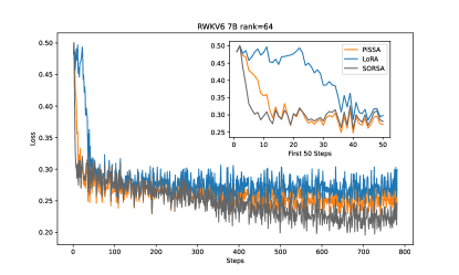
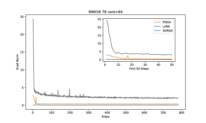
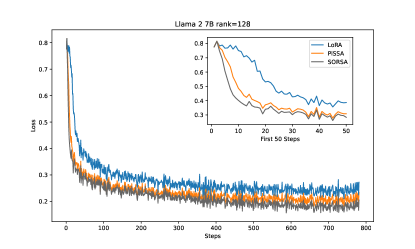
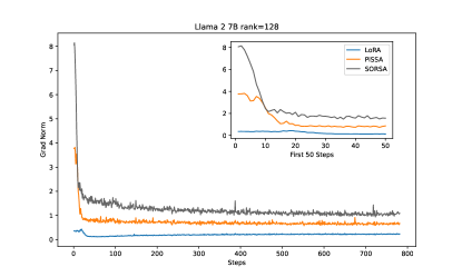
Figure 3: The training loss and gradient norm comparison between SORSA, PiSSA, and LoRA on MetaMathQA training of RWKV6 7B and Llama 2 7B. LoRA and PiSSA curves of Llama 2 7B are from Meng et al. (2024).

The results showed that across all models tested, SORSA generally outperformed other methods. For mathematical evaluations, on Llama 2 7B, SORSA scored 56.03% on GSM-8K and 10.36% on MATH, significantly outperforming other methods; For the RWKV6 7B model, SORSA achieved 45.87% accuracy on GSM-8K and 11.32% on MATH, surpassing both PiSSA and LoRA; On Mistral 7B, SORSA reached 73.09% on GSM-8K and 21.86% on MATH, slightly edging out competitors; With Gemma 7B, while SORSA’s MATH score of 29.52% was lower than LoRA and PiSSA, it still led on GSM-8K with 78.09%. Moreover, on coding evaluations, SORSA consistently achieved the highest HumanEval scores across other tuning methods, demonstrating its effectiveness on diverse natural language tasks. Noticeably, RWKV6 7B using LoRA performed extremely below our expectation in GSM-8K test. We believe this may be due to our prompt for mathematical tests (See Section B.2 for more details) are inconsistent with the model’s original prompt, causing LoRA to fail in learning this prompting behavior.

The Figure 3 reveals that while SORSA and PiSSA exhibit nearly identical loss curves at the beginning, and even a little bit higher than PiSSA on RWKV-6 training. However, when training step approximately $t>300$, SORSA continues to maintain the decrease of its loss steadily. In contrast, LoRA and PiSSA shows a deceleration in its loss reduction. This supports Theorem 5, confirming that SORSA consistently outperforms both LoRA and PiSSA, especially at later stages of training.

However, due to the limitation of computing resources, we only trained and benchmarked a small number of tasks.

7 Conclusion

In this paper, we introduced SORSA, a novel parameter-efficient fine-tuning (PEFT) method designed to enhance the adaptation of large language models (LLMs) for downstream tasks. SORSA utilizes singular value decomposition (SVD) to split pre-trained weights into principal and residual components, only training the principal singular values and vectors while freezing the residuals. We implemented an orthonormal regularizer to maintain the orthonormality of singular vectors during training, ensuring efficient parameter updates and preserving the integrity of singular values.

Our experiments demonstrated that SORSA outperforms existing PEFT methods, such as LoRA and PiSSA, in both convergence speed and accuracy on the NLG tasks. Specifically, Llama 2 7B, tuned with SORSA, achieved significant improvements in the GSM-8K and MATH benchmarks, highlighting the effectiveness of our approach.

We adopted singular values and vectors analysis, comparing SORSA with partial FT and LoRA, and we find SORSA’s superiority in preserving the pre-trained weight’s singular values and vectors during training. This suggests an explanation for SORSA’s supreme performance demonstrated in the experiment. We also show the significance of the orthonormal regularizer through analysis.

Our gradient analysis provided a mathematical foundation for SORSA, demonstrating its convexity, Lipschitz continuity, and the crucial role of the regularizer in improving the optimization landscape. This theoretical framework not only explains SORSA’s empirical superior performance but also offers valuable insights for future developments in adaptive learning algorithms.

SORSA retains the advantages of LoRA and variants, including low training VRAM requirements, no inference latency, and versatility across different neural network architectures. By offering a more efficient fine-tuning mechanism, SORSA presents a promising direction for future research and application in the field of LLMs.

Overall, SORSA gives a new perspective on parameter-efficient fine-tuning, showcasing exceptional efficiency and robust performance. It not only outperforms existing methods like LoRA and PiSSA in several downstream tasks but also maintains the practical benefits of low VRAM requirements, no inference latency, and ease of implementation. This innovative approach offers a promising direction for future research and practical applications in adapting pre-trained models, making it a pivotal development in the field.

8 Future Work

While SORSA demonstrates substantial improvements over existing PEFT methods, there are several avenues for future work to enhance its capabilities further and extend its applicability:

• Comparison Between Different Rank: Find how the performance of SORSA varies with different ranks. This investigation would help determine the optimal rank for various tasks and model sizes, potentially revealing a trade-off between computational efficiency and model performance.

• Extended Evaluation: Conduct broader evaluations of SORSA across different areas of benchmarks on models with more diverse sizes. This may able to provide a more comprehensive understanding of SORSA’s performance and versatility.

• Catastrophic Forgetting: Compare the performance of some general benchmarks like MMLU (Hendrycks et al., 2020) before and after models are adapted by SORSA in specific down-stream tasks in order to research whether SORSA could perform better than full-parameter fine-tuning, LoRA (Hu et al., 2021) or PiSSA (Meng et al., 2024) on preventing catastrophic forgetting.

• Quantization: Investigate the application of quantization techniques to SORSA similar to the approach of QLoRA (Dettmers et al., 2024) and QPiSSA (Meng et al., 2024). Quantization aims to reduce the memory footprint and computational requirements, making it feasible to deploy on devices with limited computational resources. By combining the benefits of quantization with the efficient fine-tuning capabilities of SORSA, quantization of SORSA may able to efficiently provides powerful models, which could eventually facilitate AI for a broader range of practical applications.

By pursuing these directions, future work can build on the foundation laid by SORSA, pushing the boundaries of PEFT and enhancing the adaptability and performance of large language models across a wide range of applications. This will enable the development of more versatile downstream models, potentially expanding the impact of Machine Learning into more fields and becoming an integral part of people’s everyday lives.

9 Impact Statement

In this paper, we introduced an innovative PEFT method in the area of Machine Learning. Our approach significantly streamlined the model’s tuning process, particularly for large-scale models, addressing both computational efficiency and environmental sustainability. As we push the boundaries of what is possible with Machine Learning, it is essential to consider the broader impacts of these advancements on both the environment and ethical standards within the field.

9.1 Environmental Impact

SORSA optimizes model tuning for large-scale models, reducing VRAM consumption by over 50% when adapting the Llama 3 70B Dubey et al. (2024) model than full parameter fine-tuning. This significant reduction in hardware resource requirements also suggests a less energy consumption compared to full parameter fine-tuning methods. By enhancing efficiency, our approach could significantly contributes to reducing the carbon footprint of Machine Learning operations.

9.2 Ethical Concerns

The PEFT method, while efficient, raises critical ethical concerns regarding the security of built-in safety measures in AI models. As demonstrated in Lermen & Rogers-Smith (2024), subversive fine-tuning techniques can bypass safety training intended to prevent the generation of harmful content. The ease and affordability of such methods underscore the vulnerability of safety protocols. It is imperative to develop robust safeguards that keep pace with technological advancements, ensuring that efficiency gains in model tuning do not compromise the ethical use of AI.

10 Acknowledgment

We would like to extend our gratitude to Prof. Jianyong Wang from Tsinghua University and the Computer Science Department of the Advanced Project Research Laboratory of Tsinghua University High School for providing the endorsement to the research.

Appendix A Faster SORSA Adapters

According to the definition of SORSA from Equation 7, because $\text{diag}(S_{p})$ is always a diagonal matrix, it is equivalent to:

$$\text{SORSA}(x)=xW_{r}+x(U_{p}\odot S_{p})V_{p}^{\top}$$ (14)

Where $\odot$ denotes element-wise multiplication, and $\text{diag}(W)$ denotes the diagonal elements of the matrix $W$.

This transformation allows us to reduce the computational complexity of SORSA adapters. In the original form, we have to perform twice matrix multiplications. However, in the Equation 14, we only have one matrix multiplication, and one element-wise multiplication. The time complexity of element-wise multiplication is $O(m^{2})$, which is much less than matrix multiplication’s complexity $O(m^{3})$. Therefore, while $\lim_{m\to\infty}$, the computation speed of SORSA adapters will be same as LoRA and PiSSA.

We performed a benchmark using PyTorch (Paszke et al., 2019) on a NVIDIA H100 SXM4 (80GB) GPU backed with CUDA, and Apple M2Pro CPU, in order to test the computation time between these two methods. See Figure 4 to see our results.

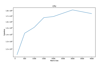
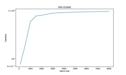
Figure 4: Benchmark between two equations of SORSA

Appendix B Experiments Details

B.1 Analysis

For the singular values and vectors analysis in Section 3, we applied partial fine-tuning, LoRA and SORSA (with and without orthonormal regularizer) on Llama 2 7B (Touvron et al., 2023) model, training with the first 100K data in MetaMathQA (Yu et al., 2024) dataset. We only calculated the loss on the response part. The models are trained with TF32 & BF16 (Wang & Kanwar, 2019) mix precision. See Table 2 for hyperparameters.

We used AdamW (Loshchilov & Hutter, 2018) optimizer and cosine annealing scheduler in training. In the analysis, LoRA and SORSA were only applied to q_proj and v_proj matrices, respectively. For Partial FT, we set model’s q_proj and v_proj matrices to trainable.

We also found we should only perform SVD for analysis using CPU, in order to get the precise analysis data.

Model	Llama 2 7B
Method	Partial FT	LoRA	SORSA (w/o reg)	SORSA
Training
Mix-Precision	TF32&BF16	TF32&BF16	TF32&BF16	TF32&BF16
Epoch	1	1	1	1
Batch Size	128	128	128	128
Max Length	512	512	512	512
Weight Decay	0	0	0	0
Warm-up Ratio	0.03	0.03	0.03	0.03
Learning Rate	2e-5	2e-5	2e-5	3e-5
Grad Clip	False	False	False	False
SORSA $\gamma$	N/A	N/A	0	5e-4
Rank	N/A	128	128	128

Table 2: Hyperparameters for the analysis

B.2 NLG Experiments

For our NLG tasks, we adapted Llama 2 7B (Touvron et al., 2023), RWKV6 7B (Peng et al., 2024), Mistral 7B v0.1 (Jiang et al., 2023) Gemma 7B (Gemma Team et al., 2024). models by SORSA. For GSM-8K (Cobbe et al., 2021) and MATH (Hendrycks et al., 2021) evaluations, we trained those models with the first 100K data in MetaMathQA (Yu et al., 2024) dataset. For HumanEval (Chen et al., 2021) evaluation, we use the first 100K data in CodeFeedback Filtered Instruction(Zheng et al., 2024) dataset.

We used AdamW (Loshchilov & Hutter, 2018) optimizer and cosine annealing scheduler in training. SORSA adapters were applied on all linear matrices in every layer. We only calculated the loss on the response part. The models are loaded in FP32, and trained with TF32 & BF16 mix precision. In our experiments, we selected a higher learning rate for SORSA compared to other methods to counterbalance the negative effect of orthonormal regularizer on optimizing toward lower training loss. See Table 3 for hyperparameters. See LABEL:lst:math for the prompt we used in GSM-8K and MATH evaluations, and LABEL:lst:humaneval for the prompt we used for HumanEval tests.

Model	Llama 2 7B	Mistral 7B	Gemma 7B	RWKV6 7B	RWKV6 7B
Method	SORSA	SORSA	SORSA	SORSA	LoRA PiSSA
Training
Mix-Precision	TF32&BF16	TF32&BF16	TF32&BF16	TF32&BF16	TF32&BF16
Epoch	1	1	1	1	1
Batch Size	128	128	128	128	128
Max Length	512	512	512	512	512
Weight Decay	0	0	0	0	0
Warm-up Ratio	0.03	0.03	0.03	0.03	0.03
Learning Rate	3e-5	3e-5	3e-5	3e-5	2e-5
Grad Clip	1.0	1.0	1.0	1.0	1.0
SORSA $\gamma$	4e-4	4e-4	4e-4	4e-4	N/A
Rank	128	64	64	64	64
Evaluating
Precision	BF16	BF16	BF16	FP32	FP32
Sampling	False
Top-P	1.0
Max Length	GSM-8K: 1024 MATH: 2048 HumanEval: 2048

Table 3: Hyperparameters of training on models for GSM-8K and MATH

⬇

1Below is an instruction that describes a task. Write a response that appropriately completes the request.

2

3### Instruction:

4{question}

5

6### Response: Let’s think step by step.

Listing 1: Prompt used for GSM-8K and MATH.

⬇

1@@ Instruction

2Here is the given code to do completion:

3‘‘‘python

4{question}

5‘‘‘

6

7Please continue to complete the function with python programming language. You are not allowed to modify the given code and do the completion only.

8

9Please return all completed codes in one code block.

10This code block should be in the following format:

11’’’python

12# Your codes here

13’’’

14

15@@ Response

Listing 2: Prompt used for HumanEval evaluation.

Appendix C Proofs

See 1

Proof.

We prove this in two steps:

First, we show that $f(U_{p})=\|U^{\top}_{p}U_{p}-I\|_{F}$ is convex. Then, we prove that $g(V_{p})=\|V_{p}V^{\top}_{p}-I\|_{F}$ is convex.

Since the sum of convex functions is convex, this will establish the convexity of ${\mathcal{L}}_{reg}$.

Let $U_{p},W\in\mathbb{R}^{m\times r}$. The Hessian of $f$ at $U_{p}$ in the direction $W$ is given by:

$$\begin{split}\nabla^{2}f(U_{p})[W,W]&=\lim_{\epsilon\to 0}\frac{1}{\epsilon^{2}}\Big{(}f(U_{p}+\epsilon W)-2f(U_{p})+f(U_{p}-\epsilon W)\Big{)}\\ &=\lim_{\epsilon\to 0}\frac{1}{\epsilon^{2}}\Big{(}\|(U_{p}+\epsilon W)^{\top}(U_{p}+\epsilon W)-I\|_{F}\\ &\quad-2\|U^{\top}_{p}U_{p}-I\|_{F}+\|(U_{p}-\epsilon W)^{\top}(U_{p}-\epsilon W)-I\|_{F}\Big{)}\\ &=\lim_{\epsilon\to 0}\frac{1}{\epsilon^{2}}\Big{(}\|U^{\top}_{p}U_{p}+\epsilon(U^{\top}_{p}W+W^{\top}U_{p})+\epsilon^{2}W^{\top}W-I\|_{F}\\ &\quad-2\|U^{\top}_{p}U_{p}-I\|_{F}+\|U^{\top}_{p}U_{p}-\epsilon(U^{\top}_{p}W+W^{\top}U_{p})+\epsilon^{2}W^{\top}W-I\|_{F}\Big{)}\\ &=2\|W^{\top}W\|_{F}\end{split}$$ (15)

Since $\|W^{\top}W\|_{F}\geq 0$ for all $W$, we have $\nabla^{2}f(U_{p})[W,W]\geq 0$, which proves that $f$ is convex.

The proof for $g(V_{p})$ follows the same steps as for $f(U_{p})$, leading to the same conclusion.

Therefore, both $f(U_{p})$ and $g(V_{p})$ are convex, and consequently, ${\mathcal{L}}_{reg}$ is convex. ∎

See 2

Proof.

To prove Lipschitz continuity, we need to show that there exists a constant $L>0$ such that for any two pairs of matrices $(U_{1},V_{1})$ and $(U_{2},V_{2})$:

$$|{\mathcal{L}}_{reg}(U_{1},V_{1})-{\mathcal{L}}_{reg}(U_{2},V_{2})|\leq L(\|U_{1}-U_{2}\|_{F}+\|V_{1}-V_{2}\|_{F})$$ (16)

Let’s break this down into two parts:

First, consider $|\|U_{1}^{\top}U_{1}-I\|_{F}-\|U_{2}^{\top}U_{2}-I\|_{F}|$:

$$\begin{split}|\|U_{1}^{\top}U_{1}-I\|_{F}-\|U_{2}^{\top}U_{2}-I\|_{F}|&\leq\|(U_{1}^{\top}U_{1}-I)-(U_{2}^{\top}U_{2}-I)\|_{F}\\ &=\|U_{1}^{\top}U_{1}-U_{2}^{\top}U_{2}\|_{F}\\ &=\|U_{1}^{\top}U_{1}-U_{1}^{\top}U_{2}+U_{1}^{\top}U_{2}-U_{2}^{\top}U_{2}\|_{F}\\ &\leq\|U_{1}^{\top}(U_{1}-U_{2})\|_{F}+\|(U_{1}^{\top}-U_{2}^{\top})U_{2}\|_{F}\\ &\leq\|U_{1}^{\top}\|_{F}\|U_{1}-U_{2}\|_{F}+\|U_{1}-U_{2}\|_{F}\|U_{2}\|_{F}\\ &\leq(\|U_{1}\|_{F}+\|U_{2}\|_{F})\|U_{1}-U_{2}\|_{F}\end{split}$$ (17)

Here, we’ve used the triangle inequality and the sub-multiplicative property of the Frobenius norm.

Similarly for $V$:

$$|\|V_{1}^{\top}V_{1}-I\|_{F}-\|V_{2}^{\top}V_{2}-I\|_{F}|\leq(\|V_{1}\|_{F}+\|V_{2}\|_{F})\|V_{1}-V_{2}\|_{F}$$ (18)

Combining these results:

$$\begin{split}|{\mathcal{L}}_{reg}(U_{1},V_{1})-{\mathcal{L}}_{reg}(U_{2},V_{2})|&\leq(\|U_{1}\|_{F}+\|U_{2}\|_{F})\|U_{1}-U_{2}\|_{F}\\ &\quad+(\|V_{1}\|_{F}+\|V_{2}\|_{F})\|V_{1}-V_{2}\|_{F}\\ &\leq\max(\|U_{1}\|_{F}+\|U_{2}\|_{F},\|V_{1}\|_{F}+\|V_{2}\|_{F})\\ &\quad\cdot(\|U_{1}-U_{2}\|_{F}+\|V_{1}-V_{2}\|_{F})\end{split}$$ (19)

Let $L_{reg}=\max(\|U_{1}\|_{F}+\|U_{2}\|_{F},\|V_{1}\|_{F}+\|V_{2}\|_{F})$. This $L$ is finite because the Frobenius norms of $U$ and $V$ are bounded (they represent orthonormal matrices in the ideal case).

Therefore, we have shown that:

$$|{\mathcal{L}}_{reg}(U_{1},V_{1})-{\mathcal{L}}_{reg}(U_{2},V_{2})|\leq L_{reg}(\|U_{1}-U_{2}\|_{F}+\|V_{1}-V_{2}\|_{F})$$ (20)

This proves that ${\mathcal{L}}_{reg}$ is Lipschitz continuous with Lipschitz constant $L_{reg}$. ∎

See 3

Proof.

For gradient descent to converge while the $\eta_{t}=\eta_{d}$, we need:

$$\eta_{d}<\frac{2}{L}=\frac{2}{L_{train}+\frac{\gamma}{\eta_{d}}L_{reg}}$$ (21)

Rearranging this inequality:

$$\begin{split}\eta_{d}(L_{train}+\frac{\gamma}{\eta_{d}}L_{reg})&<2\\ \eta_{d}L_{train}+\gamma L_{reg}&<2\\ \gamma L_{reg}&<2-\eta_{d}L_{train}\\ \gamma&<\frac{2-\eta_{d}L_{train}}{L_{reg}}\end{split}$$ (22)

We can assume that the regularizer’s gradients scale with $\eta_{d}$ , meaning that larger updating step (due to a larger $\eta_{d}$) will lead to greater deviations from orthonormality, which increases $L_{reg}$. Conversely, smaller steps lead to a more gradual progression towards orthonormality, which reduces $L_{reg}$. Therefore, we could assume $L_{reg}\propto\eta_{d}$. Moreover, the $\gamma$ must not be negative or the regularization term would impact negatively on the purposes it is supposed to have. Therefore, we can rewrite the inequality as:

$$0\leq\gamma<\frac{2}{k\eta_{d}}-L_{train}$$ (23)

This establishes the upper bound for $\gamma$. ∎

See 4

Proof.

First, let’s consider the effect of the orthonormal regularizer. The regularizer aims to make $U_{p}^{\top}U_{p}\approx I$ and $V_{p}V_{p}^{\top}\approx I$. We can quantify this approximation as:

$$\|\nabla_{W_{p}}{\mathcal{L}}_{reg}\|_{F}\leq\epsilon_{\nabla}$$ (24)

where $\epsilon_{\nabla}>0$ is a small constant.

Now, let’s consider the difference between $W_{p}^{\text{unreg}}$ and $W_{p}^{\text{reg}}$:

$$\|W_{p}^{\text{reg}}-W_{p}^{\text{unreg}}\|_{F}=\gamma\|\nabla_{W_{p}}{\mathcal{L}}_{reg}\|_{F}=\gamma\epsilon_{\nabla}$$ (25)

Now, we can use Weyl’s inequality (Weyl, 1912), which states that for matrices A and B:

$$|\sigma_{i}(A+B)-\sigma_{i}(A)|\leq\|B\|_{2}\leq\|B\|_{F}$$ (26)

Applying this to our case, with $A=W_{p}^{\text{unreg}}$ and $B=W_{p}^{\text{reg}}-W_{p}^{\text{unreg}}$:

$$|\sigma_{i}^{\text{reg}}-\sigma_{i}^{\text{unreg}}|\leq\|W_{p}^{\text{reg}}-W_{p}^{\text{unreg}}\|_{F}\leq\gamma\epsilon_{\nabla}$$ (27)

Let $\epsilon=\gamma\epsilon_{\nabla}$. Then we have:

$$-\epsilon\leq\sigma_{i}^{\text{reg}}-\sigma_{i}^{\text{unreg}}\leq\epsilon$$ (28)

Rearranging this inequality gives us our desired bound:

$$(1-\epsilon)\sigma_{i}^{\text{unreg}}\leq\sigma_{i}^{\text{reg}}\leq(1+\epsilon)\sigma_{i}^{\text{unreg}}$$ (29)

∎

See 5

Proof.

Let $W_{p}=U_{p}\text{diag}(S_{p})V_{p}^{\top}$ be the principal part of the singular value decomposition approximation of $W$. The condition number is given by:

$$\kappa(W_{p})=\frac{\sigma_{\max}(W_{p})}{\sigma_{\min}(W_{p})}$$ (30)

where $\sigma_{\max}$ and $\sigma_{\min}$ are the maximum and minimum singular values of $W_{p}$.

At initialization ($t=0$): Due to SVD initialization, $U_{p}$ and $V_{p}^{\top}$ are perfectly orthonormal, so:

$$\kappa(U_{p}^{\text{unreg}})=\kappa((V_{p}^{\text{unreg}})^{\top})=\kappa(U_{p}^{\text{reg}})=\kappa((V_{p}^{\text{reg}})^{\top})=1$$ (31)

And $\epsilon_{0}=0$, $\delta_{1,0}=\delta_{2,0}=0$. Therefore:

$$\frac{\kappa(W_{p}^{\text{reg}})}{\kappa(W_{p}^{\text{unreg}})}=\frac{\kappa(\text{diag}(S_{p})^{\text{reg}})}{\kappa(\text{diag}(S_{p})^{\text{unreg}})}=1$$ (32)

During training ($t>0$): As training progresses, $U_{p}$ and $V_{p}^{\top}$ deviate from orthonormality in the unregularized case. We quantify this deviation:

$$\|U_{p}^{\top}U_{p}-I\|_{F}\leq\epsilon_{1,t}$$ (33)

$$\|V_{p}^{\top}V_{p}-I\|_{F}\leq\epsilon_{2,t}$$ (34)

where $\epsilon_{1,t},\epsilon_{2,t}>0$ increase over time t.

For the regularized matrices, we can bound their condition numbers:

$$\kappa(U_{p}^{\text{reg}})\leq 1+\delta_{1,t}$$ (35)

$$\kappa(V_{p}^{\text{reg}})\leq 1+\delta_{2,t}$$ (36)

where $\delta_{1,t},\delta_{2,t}$ are small positive numbers that remain bounded due to the regularization.

From the Lemma 4, we arrive at:

$$\begin{split}\frac{(1+\delta_{1,t})(1+\delta_{2,t})(\frac{1-\epsilon_{t}}{1+\epsilon_{t}})}{\kappa(U_{p}^{\text{unreg}})\cdot\kappa((V_{p}^{\text{unreg}})^{\top})}\leq\frac{\kappa(W_{p}^{\text{reg}})}{\kappa(W_{p}^{\text{unreg}})}\leq\frac{(1+\delta_{1,t})(1+\delta_{2,t})(\frac{1+\epsilon_{t}}{1-\epsilon_{t}})}{\kappa(U_{p}^{\text{unreg}})\cdot\kappa((V_{p}^{\text{unreg}})^{\top})}\end{split}$$ (37)

As training continues, in the unregularized case, $\kappa(U_{p,\text{unreg}})$ and $\kappa(V_{p,\text{unreg}}^{\top})$ tend to increase as $U_{p}$ and $V_{p}^{\top}$ deviate further from orthonormality. On the other hand, $(1+\delta_{1,t})(1+\delta_{2,t})(\frac{1+\epsilon_{t}}{1-\epsilon_{t}})$ will approach to 1 because of the reinforcement in orthonormality. Therefore, $\exists c>0$, while $t>c$:

$$\kappa(U_{p}^{\text{unreg}})\cdot\kappa((V_{p}^{\text{unreg}})^{\top})>(1+\delta_{1,t})(1+\delta_{2,t})(\frac{1+\epsilon_{t}}{1-\epsilon_{t}})$$ (38)

will hold true.

Therefore, while $t>c$, we have:

$$\frac{\kappa(W_{p}^{\text{reg}})}{\kappa(W_{p}^{\text{unreg}})}<1$$ (39)

indicating an improvement in the condition number. ∎

References

- Anthony et al. (2023) Quentin Anthony, Stella Biderman, and Hailey Schoelkopf. Transformer math 101, April 2023. URL https://blog.eleuther.ai/transformer-math/.
- Arjovsky et al. (2016) Martin Arjovsky, Amar Shah, and Yoshua Bengio. Unitary evolution recurrent neural networks. In Maria Florina Balcan and Kilian Q. Weinberger (eds.), Proceedings of the 33rd international conference on machine learning, volume 48 of Proceedings of machine learning research, pp. 1120–1128, New York, New York, USA, June 2016. PMLR. URL https://proceedings.mlr.press/v48/arjovsky16.html.
- Büyükakyüz (2024) Kerim Büyükakyüz. OLoRA: Orthonormal Low-Rank Adaptation of Large Language Models, June 2024. URL https://arxiv.org/abs/2406.01775v1.
- Chen et al. (2021) Mark Chen, Jerry Tworek, Heewoo Jun, Qiming Yuan, Henrique Ponde de Oliveira Pinto, Jared Kaplan, Harri Edwards, Yuri Burda, Nicholas Joseph, Greg Brockman, Alex Ray, Raul Puri, Gretchen Krueger, Michael Petrov, Heidy Khlaaf, Girish Sastry, Pamela Mishkin, Brooke Chan, Scott Gray, Nick Ryder, Mikhail Pavlov, Alethea Power, Lukasz Kaiser, Mohammad Bavarian, Clemens Winter, Philippe Tillet, Felipe Petroski Such, Dave Cummings, Matthias Plappert, Fotios Chantzis, Elizabeth Barnes, Ariel Herbert-Voss, William Hebgen Guss, Alex Nichol, Alex Paino, Nikolas Tezak, Jie Tang, Igor Babuschkin, Suchir Balaji, Shantanu Jain, William Saunders, Christopher Hesse, Andrew N. Carr, Jan Leike, Josh Achiam, Vedant Misra, Evan Morikawa, Alec Radford, Matthew Knight, Miles Brundage, Mira Murati, Katie Mayer, Peter Welinder, Bob McGrew, Dario Amodei, Sam McCandlish, Ilya Sutskever, and Wojciech Zaremba. Evaluating Large Language Models Trained on Code, July 2021. URL http://arxiv.org/abs/2107.03374. arXiv:2107.03374 [cs].
- Cobbe et al. (2021) Karl Cobbe, Vineet Kosaraju, Mohammad Bavarian, Mark Chen, Heewoo Jun, Lukasz Kaiser, Matthias Plappert, Jerry Tworek, Jacob Hilton, Reiichiro Nakano, Christopher Hesse, and John Schulman. Training Verifiers to Solve Math Word Problems, November 2021. URL http://arxiv.org/abs/2110.14168. arXiv:2110.14168 [cs].
- Dettmers et al. (2024) Tim Dettmers, Artidoro Pagnoni, Ari Holtzman, and Luke Zettlemoyer. QLoRA: Efficient Finetuning of Quantized LLMs. Advances in Neural Information Processing Systems, 36, 2024. URL https://proceedings.neurips.cc/paper_files/paper/2023/hash/1feb87871436031bdc0f2beaa62a049b-Abstract-Conference.html.
- Dubey et al. (2024) Abhimanyu Dubey, Abhinav Jauhri, Abhinav Pandey, Abhishek Kadian, Ahmad Al-Dahle, Aiesha Letman, Akhil Mathur, Alan Schelten, Amy Yang, Angela Fan, Anirudh Goyal, Anthony Hartshorn, Aobo Yang, Archi Mitra, Archie Sravankumar, Artem Korenev, Arthur Hinsvark, Arun Rao, Aston Zhang, Aurelien Rodriguez, Austen Gregerson, Ava Spataru, Baptiste Roziere, Bethany Biron, Binh Tang, Bobbie Chern, Charlotte Caucheteux, Chaya Nayak, Chloe Bi, Chris Marra, Chris McConnell, Christian Keller, Christophe Touret, Chunyang Wu, Corinne Wong, Cristian Canton Ferrer, Cyrus Nikolaidis, Damien Allonsius, Daniel Song, Danielle Pintz, Danny Livshits, David Esiobu, Dhruv Choudhary, Dhruv Mahajan, Diego Garcia-Olano, Diego Perino, Dieuwke Hupkes, Egor Lakomkin, Ehab AlBadawy, Elina Lobanova, Emily Dinan, Eric Michael Smith, Filip Radenovic, Frank Zhang, Gabriel Synnaeve, Gabrielle Lee, Georgia Lewis Anderson, Graeme Nail, Gregoire Mialon, Guan Pang, Guillem Cucurell, Hailey Nguyen, Hannah Korevaar, Hu Xu, Hugo Touvron, Iliyan Zarov, Imanol Arrieta Ibarra, Isabel Kloumann, Ishan Misra, Ivan Evtimov, Jade Copet, Jaewon Lee, Jan Geffert, Jana Vranes, Jason Park, Jay Mahadeokar, Jeet Shah, Jelmer van der Linde, Jennifer Billock, Jenny Hong, Jenya Lee, Jeremy Fu, Jianfeng Chi, Jianyu Huang, Jiawen Liu, Jie Wang, Jiecao Yu, Joanna Bitton, Joe Spisak, Jongsoo Park, Joseph Rocca, Joshua Johnstun, Joshua Saxe, Junteng Jia, Kalyan Vasuden Alwala, Kartikeya Upasani, Kate Plawiak, Ke Li, Kenneth Heafield, Kevin Stone, Khalid El-Arini, Krithika Iyer, Kshitiz Malik, Kuenley Chiu, Kunal Bhalla, Lauren Rantala-Yeary, Laurens van der Maaten, Lawrence Chen, Liang Tan, Liz Jenkins, Louis Martin, Lovish Madaan, Lubo Malo, Lukas Blecher, Lukas Landzaat, Luke de Oliveira, Madeline Muzzi, Mahesh Pasupuleti, Mannat Singh, Manohar Paluri, Marcin Kardas, Mathew Oldham, Mathieu Rita, Maya Pavlova, Melanie Kambadur, Mike Lewis, Min Si, Mitesh Kumar Singh, Mona Hassan, Naman Goyal, Narjes Torabi, Nikolay Bashlykov, Nikolay Bogoychev, Niladri Chatterji, Olivier Duchenne, Onur Çelebi, Patrick Alrassy, Pengchuan Zhang, Pengwei Li, Petar Vasic, Peter Weng, Prajjwal Bhargava, Pratik Dubal, Praveen Krishnan, Punit Singh Koura, Puxin Xu, Qing He, Qingxiao Dong, Ragavan Srinivasan, Raj Ganapathy, Ramon Calderer, Ricardo Silveira Cabral, Robert Stojnic, Roberta Raileanu, Rohit Girdhar, Rohit Patel, Romain Sauvestre, Ronnie Polidoro, Roshan Sumbaly, Ross Taylor, Ruan Silva, Rui Hou, Rui Wang, Saghar Hosseini, Sahana Chennabasappa, Sanjay Singh, Sean Bell, Seohyun Sonia Kim, Sergey Edunov, Shaoliang Nie, Sharan Narang, Sharath Raparthy, Sheng Shen, Shengye Wan, Shruti Bhosale, Shun Zhang, Simon Vandenhende, Soumya Batra, Spencer Whitman, Sten Sootla, Stephane Collot, Suchin Gururangan, Sydney Borodinsky, Tamar Herman, Tara Fowler, Tarek Sheasha, Thomas Georgiou, Thomas Scialom, Tobias Speckbacher, Todor Mihaylov, Tong Xiao, Ujjwal Karn, Vedanuj Goswami, Vibhor Gupta, Vignesh Ramanathan, Viktor Kerkez, Vincent Gonguet, Virginie Do, Vish Vogeti, Vladan Petrovic, Weiwei Chu, Wenhan Xiong, Wenyin Fu, Whitney Meers, Xavier Martinet, Xiaodong Wang, Xiaoqing Ellen Tan, Xinfeng Xie, Xuchao Jia, Xuewei Wang, Yaelle Goldschlag, Yashesh Gaur, Yasmine Babaei, Yi Wen, Yiwen Song, Yuchen Zhang, Yue Li, Yuning Mao, Zacharie Delpierre Coudert, Zheng Yan, Zhengxing Chen, Zoe Papakipos, Aaditya Singh, Aaron Grattafiori, Abha Jain, Adam Kelsey, Adam Shajnfeld, Adithya Gangidi, Adolfo Victoria, Ahuva Goldstand, Ajay Menon, Ajay Sharma, Alex Boesenberg, Alex Vaughan, Alexei Baevski, Allie Feinstein, Amanda Kallet, Amit Sangani, Anam Yunus, Andrei Lupu, Andres Alvarado, Andrew Caples, Andrew Gu, Andrew Ho, Andrew Poulton, Andrew Ryan, Ankit Ramchandani, Annie Franco, Aparajita Saraf, Arkabandhu Chowdhury, Ashley Gabriel, Ashwin Bharambe, Assaf Eisenman, Azadeh Yazdan, Beau James, Ben Maurer, Benjamin Leonhardi, Bernie Huang, Beth Loyd, Beto De Paola, Bhargavi Paranjape, Bing Liu, Bo Wu, Boyu Ni, Braden Hancock, Bram Wasti, Brandon Spence, Brani Stojkovic, Brian Gamido, Britt Montalvo, Carl Parker, Carly Burton, Catalina Mejia, Changhan Wang, Changkyu Kim, Chao Zhou, Chester Hu, Ching-Hsiang Chu, Chris Cai, Chris Tindal, Christoph Feichtenhofer, Damon Civin, Dana Beaty, Daniel Kreymer, Daniel Li, Danny Wyatt, David Adkins, David Xu, Davide Testuggine, Delia David, Devi Parikh, Diana Liskovich, Didem Foss, Dingkang Wang, Duc Le, Dustin Holland, Edward Dowling, Eissa Jamil, Elaine Montgomery, Eleonora Presani, Emily Hahn, Emily Wood, Erik Brinkman, Esteban Arcaute, Evan Dunbar, Evan Smothers, Fei Sun, Felix Kreuk, Feng Tian, Firat Ozgenel, Francesco Caggioni, Francisco Guzmán, Frank Kanayet, Frank Seide, Gabriela Medina Florez, Gabriella Schwarz, Gada Badeer, Georgia Swee, Gil Halpern, Govind Thattai, Grant Herman, Grigory Sizov, Guangyi, Zhang, Guna Lakshminarayanan, Hamid Shojanazeri, Han Zou, Hannah Wang, Hanwen Zha, Haroun Habeeb, Harrison Rudolph, Helen Suk, Henry Aspegren, Hunter Goldman, Ibrahim Damlaj, Igor Molybog, Igor Tufanov, Irina-Elena Veliche, Itai Gat, Jake Weissman, James Geboski, James Kohli, Japhet Asher, Jean-Baptiste Gaya, Jeff Marcus, Jeff Tang, Jennifer Chan, Jenny Zhen, Jeremy Reizenstein, Jeremy Teboul, Jessica Zhong, Jian Jin, Jingyi Yang, Joe Cummings, Jon Carvill, Jon Shepard, Jonathan McPhie, Jonathan Torres, Josh Ginsburg, Junjie Wang, Kai Wu, Kam Hou U, Karan Saxena, Karthik Prasad, Kartikay Khandelwal, Katayoun Zand, Kathy Matosich, Kaushik Veeraraghavan, Kelly Michelena, Keqian Li, Kun Huang, Kunal Chawla, Kushal Lakhotia, Kyle Huang, Lailin Chen, Lakshya Garg, Lavender A, Leandro Silva, Lee Bell, Lei Zhang, Liangpeng Guo, Licheng Yu, Liron Moshkovich, Luca Wehrstedt, Madian Khabsa, Manav Avalani, Manish Bhatt, Maria Tsimpoukelli, Martynas Mankus, Matan Hasson, Matthew Lennie, Matthias Reso, Maxim Groshev, Maxim Naumov, Maya Lathi, Meghan Keneally, Michael L. Seltzer, Michal Valko, Michelle Restrepo, Mihir Patel, Mik Vyatskov, Mikayel Samvelyan, Mike Clark, Mike Macey, Mike Wang, Miquel Jubert Hermoso, Mo Metanat, Mohammad Rastegari, Munish Bansal, Nandhini Santhanam, Natascha Parks, Natasha White, Navyata Bawa, Nayan Singhal, Nick Egebo, Nicolas Usunier, Nikolay Pavlovich Laptev, Ning Dong, Ning Zhang, Norman Cheng, Oleg Chernoguz, Olivia Hart, Omkar Salpekar, Ozlem Kalinli, Parkin Kent, Parth Parekh, Paul Saab, Pavan Balaji, Pedro Rittner, Philip Bontrager, Pierre Roux, Piotr Dollar, Polina Zvyagina, Prashant Ratanchandani, Pritish Yuvraj, Qian Liang, Rachad Alao, Rachel Rodriguez, Rafi Ayub, Raghotham Murthy, Raghu Nayani, Rahul Mitra, Raymond Li, Rebekkah Hogan, Robin Battey, Rocky Wang, Rohan Maheswari, Russ Howes, Ruty Rinott, Sai Jayesh Bondu, Samyak Datta, Sara Chugh, Sara Hunt, Sargun Dhillon, Sasha Sidorov, Satadru Pan, Saurabh Verma, Seiji Yamamoto, Sharadh Ramaswamy, Shaun Lindsay, Shaun Lindsay, Sheng Feng, Shenghao Lin, Shengxin Cindy Zha, Shiva Shankar, Shuqiang Zhang, Shuqiang Zhang, Sinong Wang, Sneha Agarwal, Soji Sajuyigbe, Soumith Chintala, Stephanie Max, Stephen Chen, Steve Kehoe, Steve Satterfield, Sudarshan Govindaprasad, Sumit Gupta, Sungmin Cho, Sunny Virk, Suraj Subramanian, Sy Choudhury, Sydney Goldman, Tal Remez, Tamar Glaser, Tamara Best, Thilo Kohler, Thomas Robinson, Tianhe Li, Tianjun Zhang, Tim Matthews, Timothy Chou, Tzook Shaked, Varun Vontimitta, Victoria Ajayi, Victoria Montanez, Vijai Mohan, Vinay Satish Kumar, Vishal Mangla, Vítor Albiero, Vlad Ionescu, Vlad Poenaru, Vlad Tiberiu Mihailescu, Vladimir Ivanov, Wei Li, Wenchen Wang, Wenwen Jiang, Wes Bouaziz, Will Constable, Xiaocheng Tang, Xiaofang Wang, Xiaojian Wu, Xiaolan Wang, Xide Xia, Xilun Wu, Xinbo Gao, Yanjun Chen, Ye Hu, Ye Jia, Ye Qi, Yenda Li, Yilin Zhang, Ying Zhang, Yossi Adi, Youngjin Nam, Yu, Wang, Yuchen Hao, Yundi Qian, Yuzi He, Zach Rait, Zachary DeVito, Zef Rosnbrick, Zhaoduo Wen, Zhenyu Yang, and Zhiwei Zhao. The Llama 3 Herd of Models, August 2024. URL http://arxiv.org/abs/2407.21783. arXiv:2407.21783 [cs].
- Gemma Team et al. (2024) Gemma Team, Thomas Mesnard, Cassidy Hardin, Robert Dadashi, Surya Bhupatiraju, Shreya Pathak, Laurent Sifre, Morgane Rivière, Mihir Sanjay Kale, Juliette Love, Pouya Tafti, Léonard Hussenot, Pier Giuseppe Sessa, Aakanksha Chowdhery, Adam Roberts, Aditya Barua, Alex Botev, Alex Castro-Ros, Ambrose Slone, Amélie Héliou, Andrea Tacchetti, Anna Bulanova, Antonia Paterson, Beth Tsai, Bobak Shahriari, Charline Le Lan, Christopher A. Choquette-Choo, Clément Crepy, Daniel Cer, Daphne Ippolito, David Reid, Elena Buchatskaya, Eric Ni, Eric Noland, Geng Yan, George Tucker, George-Christian Muraru, Grigory Rozhdestvenskiy, Henryk Michalewski, Ian Tenney, Ivan Grishchenko, Jacob Austin, James Keeling, Jane Labanowski, Jean-Baptiste Lespiau, Jeff Stanway, Jenny Brennan, Jeremy Chen, Johan Ferret, Justin Chiu, Justin Mao-Jones, Katherine Lee, Kathy Yu, Katie Millican, Lars Lowe Sjoesund, Lisa Lee, Lucas Dixon, Machel Reid, Maciej Mikuła, Mateo Wirth, Michael Sharman, Nikolai Chinaev, Nithum Thain, Olivier Bachem, Oscar Chang, Oscar Wahltinez, Paige Bailey, Paul Michel, Petko Yotov, Rahma Chaabouni, Ramona Comanescu, Reena Jana, Rohan Anil, Ross McIlroy, Ruibo Liu, Ryan Mullins, Samuel L. Smith, Sebastian Borgeaud, Sertan Girgin, Sholto Douglas, Shree Pandya, Siamak Shakeri, Soham De, Ted Klimenko, Tom Hennigan, Vlad Feinberg, Wojciech Stokowiec, Yu-hui Chen, Zafarali Ahmed, Zhitao Gong, Tris Warkentin, Ludovic Peran, Minh Giang, Clément Farabet, Oriol Vinyals, Jeff Dean, Koray Kavukcuoglu, Demis Hassabis, Zoubin Ghahramani, Douglas Eck, Joelle Barral, Fernando Pereira, Eli Collins, Armand Joulin, Noah Fiedel, Evan Senter, Alek Andreev, and Kathleen Kenealy. Gemma: Open Models Based on Gemini Research and Technology, April 2024. URL http://arxiv.org/abs/2403.08295. arXiv:2403.08295 [cs].
- He et al. (2022) Junxian He, Chunting Zhou, Xuezhe Ma, Taylor Berg-Kirkpatrick, and Graham Neubig. Towards a Unified View of Parameter-Efficient Transfer Learning, February 2022. URL http://arxiv.org/abs/2110.04366. arXiv:2110.04366 [cs].
- Hendrycks et al. (2020) Dan Hendrycks, Collin Burns, Steven Basart, Andy Zou, Mantas Mazeika, Dawn Song, and Jacob Steinhardt. Measuring Massive Multitask Language Understanding. In International Conference on Learning Representations, October 2020. URL https://openreview.net/forum?id=d7KBjmI3GmQ.
- Hendrycks et al. (2021) Dan Hendrycks, Collin Burns, Saurav Kadavath, Akul Arora, Steven Basart, Eric Tang, Dawn Song, and Jacob Steinhardt. Measuring Mathematical Problem Solving With the MATH Dataset. In Thirty-fifth Conference on Neural Information Processing Systems Datasets and Benchmarks Track (Round 2), August 2021. URL https://openreview.net/forum?id=7Bywt2mQsCe.
- Houlsby et al. (2019) Neil Houlsby, Andrei Giurgiu, Stanislaw Jastrzebski, Bruna Morrone, Quentin De Laroussilhe, Andrea Gesmundo, Mona Attariyan, and Sylvain Gelly. Parameter-Efficient Transfer Learning for NLP. In International conference on machine learning, pp. 2790–2799. PMLR, 2019. URL http://proceedings.mlr.press/v97/houlsby19a.html.
- Hu et al. (2021) Edward J. Hu, Yelong Shen, Phillip Wallis, Zeyuan Allen-Zhu, Yuanzhi Li, Shean Wang, Lu Wang, and Weizhu Chen. LoRA: Low-Rank Adaptation of Large Language Models. In International Conference on Learning Representations, October 2021. URL https://openreview.net/forum?id=nZeVKeeFYf9.
- Huang et al. (2018) Lei Huang, Xianglong Liu, Bo Lang, Adams Yu, Yongliang Wang, and Bo Li. Orthogonal Weight Normalization: Solution to Optimization Over Multiple Dependent Stiefel Manifolds in Deep Neural Networks. Proceedings of the AAAI Conference on Artificial Intelligence, 32(1), April 2018. ISSN 2374-3468, 2159-5399. doi: 10.1609/aaai.v32i1.11768. URL https://ojs.aaai.org/index.php/AAAI/article/view/11768.
- Jiang et al. (2023) Albert Q. Jiang, Alexandre Sablayrolles, Arthur Mensch, Chris Bamford, Devendra Singh Chaplot, Diego de las Casas, Florian Bressand, Gianna Lengyel, Guillaume Lample, Lucile Saulnier, Lélio Renard Lavaud, Marie-Anne Lachaux, Pierre Stock, Teven Le Scao, Thibaut Lavril, Thomas Wang, Timothée Lacroix, and William El Sayed. Mistral 7B, October 2023. URL http://arxiv.org/abs/2310.06825. arXiv:2310.06825 [cs].
- Lermen & Rogers-Smith (2024) Simon Lermen and Charlie Rogers-Smith. LoRA Fine-tuning Efficiently Undoes Safety Training in Llama 2-Chat 70B. In ICLR 2024 Workshop on Secure and Trustworthy Large Language Models, April 2024. URL https://openreview.net/forum?id=Y52UbVhglu.
- Lester et al. (2021) Brian Lester, Rami Al-Rfou, and Noah Constant. The Power of Scale for Parameter-Efficient Prompt Tuning. In Proceedings of the 2021 Conference on Empirical Methods in Natural Language Processing, pp. 3045–3059. arXiv, 2021. arXiv:2104.08691 [cs].
- Lin et al. (2020) Zhaojiang Lin, Andrea Madotto, and Pascale Fung. Exploring Versatile Generative Language Model Via Parameter-Efficient Transfer Learning. In Trevor Cohn, Yulan He, and Yang Liu (eds.), Findings of the Association for Computational Linguistics: EMNLP 2020, pp. 441–459, Online, November 2020. Association for Computational Linguistics. doi: 10.18653/v1/2020.findings-emnlp.41. URL https://aclanthology.org/2020.findings-emnlp.41.
- Liu et al. (2024) Shih-yang Liu, Chien-Yi Wang, Hongxu Yin, Pavlo Molchanov, Yu-Chiang Frank Wang, Kwang-Ting Cheng, and Min-Hung Chen. DoRA: Weight-Decomposed Low-Rank Adaptation. In Forty-first International Conference on Machine Learning, June 2024. URL https://openreview.net/forum?id=3d5CIRG1n2&referrer=%5Bthe%20profile%20of%20Chien-Yi%20Wang%5D(%2Fprofile%3Fid%3D~Chien-Yi_Wang1).
- Liu et al. (2022) Xiao Liu, Kaixuan Ji, Yicheng Fu, Weng Lam Tam, Zhengxiao Du, Zhilin Yang, and Jie Tang. P-Tuning v2: Prompt Tuning Can Be Comparable to Fine-tuning Universally Across Scales and Tasks, March 2022. URL http://arxiv.org/abs/2110.07602. arXiv:2110.07602 [cs].
- Loshchilov & Hutter (2018) Ilya Loshchilov and Frank Hutter. Decoupled Weight Decay Regularization. In International Conference on Learning Representations, 2018. URL https://openreview.net/forum?id=Bkg6RiCqY7.
- Meng et al. (2024) Fanxu Meng, Zhaohui Wang, and Muhan Zhang. PiSSA: Principal Singular Values and Singular Vectors Adaptation of Large Language Models, April 2024. URL http://arxiv.org/abs/2404.02948. arXiv:2404.02948 [cs].
- OpenAI (2023) OpenAI. GPT-4 Technical Report, March 2023. URL http://arxiv.org/abs/2303.08774. arXiv:2303.08774 [cs].
- Pan et al. (2024) Rui Pan, Xiang Liu, Shizhe Diao, Renjie Pi, Jipeng Zhang, Chi Han, and Tong Zhang. LISA: Layerwise Importance Sampling for Memory-Efficient Large Language Model Fine-Tuning. arXiv preprint arXiv:2403.17919, 2024. URL https://arxiv.org/abs/2403.17919.
- Paszke et al. (2019) Adam Paszke, Sam Gross, Francisco Massa, Adam Lerer, James Bradbury, Gregory Chanan, Trevor Killeen, Zeming Lin, Natalia Gimelshein, Luca Antiga, Alban Desmaison, Andreas Kopf, Edward Yang, Zachary DeVito, Martin Raison, Alykhan Tejani, Sasank Chilamkurthy, Benoit Steiner, Lu Fang, Junjie Bai, and Soumith Chintala. PyTorch: An Imperative Style, High-Performance Deep Learning Library. In Advances in Neural Information Processing Systems, volume 32. Curran Associates, Inc., 2019. URL https://proceedings.neurips.cc/paper/2019/hash/bdbca288fee7f92f2bfa9f7012727740-Abstract.html.
- Peng et al. (2024) Bo Peng, Daniel Goldstein, Quentin Anthony, Alon Albalak, Eric Alcaide, Stella Biderman, Eugene Cheah, Teddy Ferdinan, Haowen Hou, Przemysław Kazienko, Kranthi Kiran GV, Jan Kocoń, Bartłomiej Koptyra, Satyapriya Krishna, Ronald McClelland Jr., Niklas Muennighoff, Fares Obeid, Atsushi Saito, Guangyu Song, Haoqin Tu, Stanisław Woźniak, Ruichong Zhang, Bingchen Zhao, Qihang Zhao, Peng Zhou, Jian Zhu, and Rui-Jie Zhu. Eagle and Finch: RWKV with Matrix-Valued States and Dynamic Recurrence, April 2024. URL http://arxiv.org/abs/2404.05892. arXiv:2404.05892 [cs].
- Radford et al. (2019) Alec Radford, Jeffrey Wu, Rewon Child, David Luan, Dario Amodei, and Ilya Sutskever. Language Models are Unsupervised Multitask Learners, 2019.
- Razdaibiedina et al. (2023) Anastasia Razdaibiedina, Yuning Mao, Rui Hou, Madian Khabsa, Mike Lewis, Jimmy Ba, and Amjad Almahairi. Residual Prompt Tuning: Improving Prompt Tuning with Residual Reparameterization, May 2023. URL http://arxiv.org/abs/2305.03937. arXiv:2305.03937 [cs].
- Saxe et al. (2014) Andrew M. Saxe, James L. McClelland, and Surya Ganguli. Exact solutions to the nonlinear dynamics of learning in deep linear neural networks, February 2014. URL http://arxiv.org/abs/1312.6120. arXiv:1312.6120 [cond-mat, q-bio, stat].
- Touvron et al. (2023) Hugo Touvron, Louis Martin, Kevin Stone, Peter Albert, Amjad Almahairi, Yasmine Babaei, Nikolay Bashlykov, Soumya Batra, Prajjwal Bhargava, Shruti Bhosale, Dan Bikel, Lukas Blecher, Cristian Canton Ferrer, Moya Chen, Guillem Cucurull, David Esiobu, Jude Fernandes, Jeremy Fu, Wenyin Fu, Brian Fuller, Cynthia Gao, Vedanuj Goswami, Naman Goyal, Anthony Hartshorn, Saghar Hosseini, Rui Hou, Hakan Inan, Marcin Kardas, Viktor Kerkez, Madian Khabsa, Isabel Kloumann, Artem Korenev, Punit Singh Koura, Marie-Anne Lachaux, Thibaut Lavril, Jenya Lee, Diana Liskovich, Yinghai Lu, Yuning Mao, Xavier Martinet, Todor Mihaylov, Pushkar Mishra, Igor Molybog, Yixin Nie, Andrew Poulton, Jeremy Reizenstein, Rashi Rungta, Kalyan Saladi, Alan Schelten, Ruan Silva, Eric Michael Smith, Ranjan Subramanian, Xiaoqing Ellen Tan, Binh Tang, Ross Taylor, Adina Williams, Jian Xiang Kuan, Puxin Xu, Zheng Yan, Iliyan Zarov, Yuchen Zhang, Angela Fan, Melanie Kambadur, Sharan Narang, Aurelien Rodriguez, Robert Stojnic, Sergey Edunov, and Thomas Scialom. Llama 2: Open Foundation and Fine-Tuned Chat Models, July 2023. URL http://arxiv.org/abs/2307.09288. arXiv:2307.09288 [cs].
- Wang & Kanwar (2019) Shibo Wang and Pankaj Kanwar. BFloat16: The secret to high performance on Cloud TPUs, August 2019. URL https://cloud.google.com/blog/products/ai-machine-learning/bfloat16-the-secret-to-high-performance-on-cloud-tpus.
- Weyl (1912) Hermann Weyl. Das asymptotische Verteilungsgesetz der Eigenwerte linearer partieller Differentialgleichungen (mit einer Anwendung auf die Theorie der Hohlraumstrahlung). Mathematische Annalen, 71(4):441–479, December 1912. ISSN 0025-5831, 1432-1807. doi: 10.1007/BF01456804. URL http://link.springer.com/10.1007/BF01456804.
- Wisdom et al. (2016) Scott Wisdom, Thomas Powers, John Hershey, Jonathan Le Roux, and Les Atlas. Full-Capacity Unitary Recurrent Neural Networks. In Advances in Neural Information Processing Systems, volume 29. Curran Associates, Inc., 2016. URL https://proceedings.neurips.cc/paper_files/paper/2016/hash/d9ff90f4000eacd3a6c9cb27f78994cf-Abstract.html.
- Yu et al. (2024) Longhui Yu, Weisen Jiang, Han Shi, Jincheng Yu, Zhengying Liu, Yu Zhang, James Kwok, Zhenguo Li, Adrian Weller, and Weiyang Liu. MetaMath: Bootstrap Your Own Mathematical Questions for Large Language Models. In The Twelfth International Conference on Learning Representations, 2024. URL https://openreview.net/forum?id=N8N0hgNDRt.
- Zhang et al. (2023) Qingru Zhang, Minshuo Chen, Alexander Bukharin, Pengcheng He, Yu Cheng, Weizhu Chen, and Tuo Zhao. Adaptive Budget Allocation for Parameter-Efficient Fine-Tuning. In The Eleventh International Conference on Learning Representations, 2023. URL https://openreview.net/forum?id=lq62uWRJjiY.
- Zhao et al. (2024) Jiawei Zhao, Zhenyu Zhang, Beidi Chen, Zhangyang Wang, Anima Anandkumar, and Yuandong Tian. GaLore: Memory-Efficient LLM Training by Gradient Low-Rank Projection. In Forty-first International Conference on Machine Learning, June 2024. URL https://openreview.net/forum?id=hYHsrKDiX7.
- Zheng et al. (2024) Tianyu Zheng, Ge Zhang, Tianhao Shen, Xueling Liu, Bill Yuchen Lin, Jie Fu, Wenhu Chen, and Xiang Yue. OpenCodeInterpreter: Integrating Code Generation with Execution and Refinement, February 2024. URL http://arxiv.org/abs/2402.14658. arXiv:2402.14658 [cs].