Signatures of topology in generic transport measurements for Rarita-Schwinger-Weyl semimetals

Abstract

We investigate how the signatures of the topological properties of the bandstructures for nodal-point semimetals are embedded in the response coefficients, arising in two distinct experimental set-ups, by taking the Rarita-Schwinger-Weyl semimetal as an example. The first scenario involves the computation of third-rank tensors representing second-order response coefficients, relating the charge/thermal current densities to the combined effects of the gradient of the chemical potential and an external electric field/temperature gradient. On the premises that internode scatterings can be ignored, the relaxation-time approximation leads to a quantized value for the nonvanishing components of each of these nonlinear response tensors, characterizing a single untilted RSW node. Furthermore, the final expressions turn out to be insensitive to the specific values of the chemical potential and the temperature. The second scenario involves computing the magnetoelectric conductivity under the action of collinear electric ($\mathbf{E}$) and magnetic ($\mathbf{B}$) fields, representing a planar Hall set-up. In particular, our focus is in bringing out the dependence of the linear-in-$|\mathbf{B}|$ parts of the conductivity tensor on the intrinsic topological properties of the bandstructure, which are nonvanishing only in the presence of a nonzero tilt in the energy spectrum.

I Introduction

Three-dimensional (3d) topological semimetals [1, 2, 3, 4] form the gapless cousins of the topological insulators, possessing a gapless spectrum, which a gap-opening implying a topological phase transition. Weyl semimetals (WSMs) exemplify such topological phases, forming an intermediate state in the transition from metals to insulators, in which the conduction and the valence bands touch only at discrete points. This leads to the emergence of zero band-gap and singular points in the Brillouin zone (BZ), known as nodal points, where the density-of-states vanish exactly. The nodal are topologically stable as they cannot be fully gapped out by perturbations that are small (in magnitude) and local in momentum space, such that the bulk gap remains intact sufficiently away from the band-crossing points. The stability of the nodal points and, consequently, the gaplessness of the semimetallic phases are ensured by the fact these points act as the sources/sinks of topological charges (leading to the noting of defective or singular points). Although the topological charges are determined by the electronic bandstructure of the material, often they are not directly measurable. However, two experimentally-accessible and exploitable properties that appear are:

1. Quantized response in various transport measurements that depend on the intrinsic Berry curvature (BC) of the bandstructures. Some examples include circular dichroism [5, 6], circular photogalvanic effect [7, 8, 9, 10], and Magnus Hall effect [11, 12, 13].

2. Fermi arcs surface states at the two-dimensional (2d) surface BZ [3].

Although not in the form of a quantized response, the signatures of BC are very much present in numerous other transport properties, such as intrinsic anomalous Hall effect [14, 15, 16], planar Hall effects [17, 18, 19, 20, 21, 22, 23, 24, 25, 26, 27, 28, 29, 30, 31, 32, 33, 34, 35, 36], magneto-optical conductivity with strong (quantizing) magnetic field [37, 38, 39], transmission of quasiparticles across barriers/wells of electric potential [40, 41, 42, 43, 44].

In the WSMs [1, 2], we encounter twofold band-crossing singularities, with each band having an isotropic linear-in-momentum dispersion in the vicinity of the nodal point. The 230 space groups in nonrelativistic condensed matter physics allows the possibility of richer bandstructures in the form symmetry-protected multifold band-crossings [45]. The simplest case is the one where each band exhibits an isotropic linear-in-momentum dispersion, akin to the WSMs. In general, the effective low-energy Hamiltonian of such a system is captured by $\sim\mathbf{k}\cdot\bm{\mathcal{S}}$, where $\bm{\mathcal{S}}$ is the vector operator comprising the three components of the angular momentum in the spin-$\varsigma$ representation of the SO(3) group. This stems from the $(2\,\varsigma+1)$ bands touching at the nodal point, resulting in the itinerant electronic degrees of freedom represented by quasiparticles with pseudospin quantum numbers equalling $\varsigma$. The terminology of “pseudospin” is used in order to clearly demarcate it as a quantum number distinct from the relativistic spin of an electron. While WSMs feature $\varsigma=1/2$, the poster child for multifold cases is the Rarita-Schwinger-Weyl (RSW) semimetal [45, 46, 47, 48, 49, 50, 51, 5, 52, 13, 44, 53, 36], having pseudospin-3/2 (i.e., fourfold band-crossings). This nomenclature is inspired by the fact that in the branch of theoretical high-energy physics, the Rarita-Schwinger (RS) equation describes the field equation of elementary particles with the relativistic spin of 3/2, which naturally arise in supergravity models [54]. Albeit, these higher-spin fermionic particles appear neither in the standard model of particle physics, nor has been detected experimentally. The RSW semimetals thus present a nonrelativistic analogoue of the elusive RS fermions in the context of solid-state systems.

Let us now elaborate on the origins of the BC and the quantized-response phenonmena in widely different experimental settings. The topological properties of a crystalline bandstructure are inferred by treating the BZ as a closed manifold. A nodal-point semimetal is endowed with a nontrivial topology when the nodes demarcate point-like topological defects, mathematically quantified as the locations of the BC monopoles [55, 4]. The charge of a BC monopole, therefore, is a topological charge, whose sign assigns a chirality $\chi$ to the node, with $\chi=+1$ and $\chi=-1$ labelling the so-called right-moving and left-moving chiral quasiparticles, respectively. The physical picture thus represents that a positively-charged (negatively-charged) monopole acts as a source (sink) for the BC flux lines. The singular points always appear in pairs, with each pair having opposite values of $\chi$, thus satisfying the Nielson-Ninomiya theorem [56]. Here, we will adopt the widely-used convention of assigning $\chi=1$ to the bands with negative energy (with respect to the band-crossing point). Using all the above definitions, we find that the monopole charge of a specific band is computed by employing the familiar Gauss’s law, where we integrate the BC flux over a closed 2d surface enclosing the point-defect. If we project on to the space of a pair of bands with the same magnitide of the pseudospin magnetic quantum numbers, we get a two-level system — the Chern number ($\mathcal{C}$) represents a wrapping number of the map from the 2d closed surface (topologically equivalent to $S^{2}$) to the Bloch sphere ($S^{2}$), given by the elements of the second homotopy group $\Pi_{2}(S^{2})=\mathbb{Z}$. Thus the monopole charges are equivalent to the Chern numbers, when interpreted as the wrapping numbers of the defects. Our aim in this paper is to unravel some transport coefficients for the RSW nodes, which show a quantized nature, being proportional to $\mathcal{C}$, thus revealing the nature of the underlying topology. In this context, it is necessary to point out that the four bands at a single RSW node have Chern numbers $\pm 1$ and $\pm 3$, which sum up to a net monopole charge of magnitude 4 (considering either the two upper or the two lower bands). Therefore, while a WSM-node harbours a Berry monopole charge of magnitude unity, an RSW hosts a net monopole charge of a higher-integer value. In this paper, we will show how these higher values of charges may show up as quantized response in various experimental set-ups. In fact, the signatures of the existence of RSW quasiparticles are believed to be reflected by the large values of the topological charges detected in a range of materials, such as $\mathrm{CoSi}$ [57], $\mathrm{RhSi}$ [58], $\mathrm{AlPt}$ [59], and $\mathrm{PdBiSe}$ [60].

In this paper, we consider the quantization associated with two distinct experimental set-ups:

1. Nonlinear transport under the effect of an external electric field (and/or temperature gradient) and the gradient of the chemical potential, constituting a response of electrochemical (or thermochemical) nature [61]. Here, we dub the associated electrical and thermal conductivity tensors as the electrochemical response (ECR) and thermochemical response (TCR), respectively. For a single untilted node of WSM, the ECR has been shown to take quantized values for temperature $T$ equalling zero [61]. However, there were various shortcomings in their steps to derive the form of the response, which we will clarify in the course of our computations. Moreover, we will show the quantized nature of both the ECR and the TCR considering at a generic temperature (albeit with $T\ll 1$) for the fourfold nodal point of the RSW, which is a multiband generalization of the WSM case.

2. Components of the magnetoelectric conductivity under the action of electric ($\mathbf{E}$) and magnetic ($\mathbf{B}$) fields, applied parallel to each other, constituting a planar Hall set-up. Here, we will demonstrate the quantized nature of the linear-in-$B$ parts of the linear-response tensor, arising from the the four bands of an RSW node.

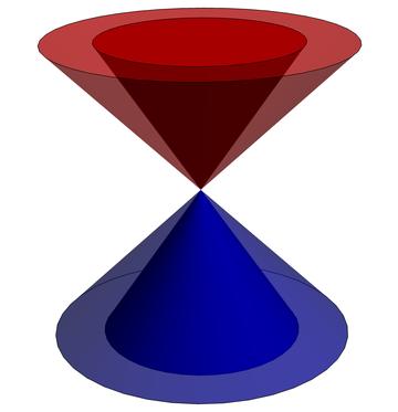
Figure 1: Schematics of the dispersions of the four bands at a single untilted node of an RSW semimetal. Each band takes a conical shape when the energy eigenvalues are plotted against the $k_{x}k_{y}$-, $k_{y}k_{z}$-, or $k_{z}k_{x}$-plane.

The paper is organized as follows. In Sec. II, we outline the form of the low-energy effective Hamiltonian in the vicinity of an RSW node and, also, show the expressions for various topological quantities. Sec. III is devoted to the review of the semiclassical Boltzmann equations. While Sec. IV deals with the nonlinear response coefficients dubbed as ECR and TCR, Sec. V focusses on the linear response associated with the magnetoelectric conductivity. In the end, we wrap up with a summary and outlook in Sec. VI. The appendices are devoted to elaborating on some the details of the intermediate steps, necessary to derive the final expressions shown in the main text. In all our expressions, we resort to using the natural units, which implies that the reduced Planck’s constant ($\hbar$), the speed of light ($c$), and the Boltzmann constant ($k_{B}$) are each set to unity.

II Model

With the help of group-theoretic symmetry analysis and first principles calculations, it has been shown that seven space groups may host fourfold band-crossing points [45] at high symmetry points of the BZ. Nearly 40 candidate materials have also been identified that can host the resulting RSW quasiparticles. The usual method of linearizing the $\mathbf{k}\cdot\mathbf{p}$ Hamiltonian about such a degeneracy point provides us with the low-energy effective continuum Hamiltonian, valid in the vicinity of the node. The explicit form of this Hamiltonian, for a single node with chirality $\chi$, is given by

$$\mathcal{H}(\mathbf{k})=\zeta\,v_{0}\,k_{z}+\chi\,v_{0}\left(k_{x}\,{\mathcal{J}}_{x}+k_{y}\,{\mathcal{J}}_{y}+k_{z}\,{\mathcal{J}}_{z}\right),$$ (1)

where $\bm{\mathcal{J}}=\{{\mathcal{J}}_{x},\,{\mathcal{J}}_{y},\,{\mathcal{J}}_{z}\}$ represents the vector operator whose three components comprise the the angular momentum operators in the spin-$3/2$ representation of the SO(3) group. We choose the commonly-used representation where

$${\mathcal{J}}_{x}=\begin{pmatrix}0&\frac{\sqrt{3}}{2}&0&0\\ \frac{\sqrt{3}}{2}&0&1&0\\ 0&1&0&\frac{\sqrt{3}}{2}\\ 0&0&\frac{\sqrt{3}}{2}&0\end{pmatrix},\quad{\mathcal{J}}_{y}=\begin{pmatrix}0&\frac{-i\,\sqrt{3}}{2}&0&0\\ \frac{i\,\sqrt{3}}{2}&0&-i&0\\ 0&i&0&\frac{-i\,\sqrt{3}}{2}\\ 0&0&\frac{i\,\sqrt{3}}{2}&0\end{pmatrix},\quad{\mathcal{J}}_{z}=\begin{pmatrix}\frac{3}{2}&0&0&0\\ 0&\frac{1}{2}&0&0\\ 0&0&-\frac{1}{2}&0\\ 0&0&0&-\frac{3}{2}\end{pmatrix}.$$ (2)

Our convention is such that the pair of conjugate nodes are separated along the $k_{z}$-direction. The energy eigenvalues are found to be

$$\varepsilon_{s}(k)=s\,v_{0}\,k\,,\quad s\in\left\{\pm\frac{1}{2},\pm\frac{3}{2}\right\},$$ (3)

where $k=\sqrt{k_{x}^{2}+k_{y}^{2}+k_{z}^{2}}$. Hence, each of four bands has an isotropic linear-in-momentum dispersion (cf. Fig. 1). The signs of “$+$” and “$-$” give us the dispersion relations for the conduction and valence bands, respectively. The corresponding group velocities of the quasiparticles are given by

$$\bm{v}_{s}(\mathbf{k}) =\nabla_{\mathbf{k}}\varepsilon_{s}(\mathbf{k})=\frac{s\,v_{0}\,\mathbf{k}}{k}+\eta\,v_{0}\,{\mathbf{\hat{k}_{z}}}\,.$$ (4)

II.1 Properties with topological origins

A nontrivial topology of the bandstructure of the RSW semimetals gives wise to the BC and the orbital magnetic moment (OMM), using the starting expressions of [62]

$${\mathbf{\Omega}}_{s}(\mathbf{k}) =i\,\langle\nabla_{\mathbf{k}}\psi_{s}({\mathbf{k}})|\,\crossproduct\,|\nabla_{\mathbf{k}}\psi_{s}({\mathbf{k}})\rangle\text{ and }\mathbf{m}_{s}(\mathbf{k})=-\,\frac{e}{2}\,\text{Im}\left[\langle\nabla_{\mathbf{k}}\psi_{s}|\crossproduct\left(\mathcal{H}{(\mathbf{k})}-\varepsilon_{s}(\mathbf{k})\right)|\nabla_{\mathbf{k}}\psi_{s}\rangle\right],$$ (5)

respectively. Here, $|\psi_{s}({\mathbf{k}})\rangle$ denotes the eigenfunction for the $s^{\rm th}$ band at the node with chirality $\chi$, and $e$ denotes the magnitude of the charge of a single electron. Evaluating these expressions for the RSW node described by $\mathcal{H}(\mathbf{k})$, we get

$${\mathbf{\Omega}}_{s}(\mathbf{k}) =-\,\frac{\chi\,s\,\mathbf{k}}{k^{3}}\text{ and }\mathbf{m}_{s}(\mathbf{k})=-\,\frac{e\,\chi\,v_{0}\,\mathcal{G}_{s}\,\mathbf{k}}{k^{2}}\,,\text{ with }\mathcal{G}_{\pm\frac{3}{2}}=\frac{3}{4}\text{ and }\mathcal{G}_{\pm\frac{1}{2}}=\frac{7}{4}\,.$$ (6)

Since $\mathbf{\Omega}_{s}(\mathbf{k})$ and $\mathbf{m}_{s}(\mathbf{k})$ are the intrinsic properties of the bandstructure, they depend only on the wavefunctions. Clearly, they are related as

$$\mathbf{m}_{s}(\mathbf{k})=\frac{e\,v_{0}\,\mathcal{G}_{s}\,k}{s}\,{\mathbf{\Omega}}_{s}(\mathbf{k})\,.$$ (7)

We observe that, unlike the BC, the OMM does not depend on the sign of the energy dispersion.

The OMM behaves exactly like the electron spin, because, on applying a magnetic field $\mathbf{B}$, it couples to the field through a Zeeman-like term, quantified by

$$\zeta_{s}({\mathbf{k}}) =-\,\mathbf{m}_{s}(\mathbf{k})\cdot\mathbf{B}=e\,\chi\,v_{0}\,\mathcal{G}_{s}\,\frac{\mathbf{k}\cdot\mathbf{B}}{k^{2}}\,.$$ (8)

Therefore, we have

$$\xi_{s}({\mathbf{k}}) =\varepsilon_{s}(\mathbf{k})+\zeta_{s}(\mathbf{k})\,,\quad\bm{w}_{s}(\mathbf{k})=\bm{v}_{s}(\mathbf{k})+\bm{u}_{s}(\mathbf{k})\,,\quad\bm{u}_{s}(\mathbf{k})=\nabla_{\mathbf{k}}\zeta_{s}(\mathbf{k})=e\,\chi\,v_{0}\,\mathcal{G}_{s}\,\frac{\mathbf{B}-2\,\hat{{\mathbf{k}}}\left(\hat{{\mathbf{k}}}\cdot\mathbf{B}\right)}{k^{2}}\,,$$ (9)

where $\xi_{s}({\mathbf{k}})$ and $\bm{w}_{s}(\mathbf{k})$ are the OMM-modified energy and band velocity of the quasiparticles, respectively. With the usual usage of notations, $\hat{\mathbf{k}}$ is the unit vector along $\mathbf{k}$. The full rotational isotropy of the Fermi surface, for each band of the RSW node, is broken by the inclusion of the OMM corrections.

II.2 Chern numbers

Using Eq. (6), the Chern number for the $s^{\rm th}$ band can be evaluated as

$$\mathcal{C}_{s}=\frac{1}{2\,\pi}\int_{S}d\mathbf{S}\cdot{\mathbf{\Omega}}_{s}\,,$$ (10)

where $S$ denotes a closed surface enclosing the $\mathbf{k}=\mathbf{0}$ point and $d\mathbf{S}$ denotes the outwardly-directed area vector for an infinitesimal patch on $S$. Exploiting the spherical symmetry of the Fermi surfaces for the bands of an isotropic RSW node, we can choose $S$ to be the surface of a unit sphere. Expressing in terms of the spherical polar coordinates, we use $k_{x}=\sin\theta\cos\phi$, $k_{y}=\sin\theta\sin\phi\sin\theta$, and $k_{z}=\cos\theta$, which gives us $d\mathbf{S}=\sin\theta\,d\theta\,d\phi\,{\mathbf{\hat{k}}}$. This leads to

$$\mathcal{C}_{s}=-\,\frac{\chi\,s}{2\,\pi}\int_{S}d\theta\,d\phi\sin\theta=-\,2\,\chi\,s\,.$$ (11)

III Response using the Boltzmann equations

In this section, we will review the semiclassical Boltzmann equation (BE) formalism used in our earlier papers, viz. [34, 32, 36], which is the widely-used framework for determining the transport coefficients in the regime of small deviations from the equilibrium quasiparticle distribution. If there is an externally-applied magnetic field $\mathbf{B}$, then we will we assume that it is of small in magnitude, associated with a small cyclotron frequency $\omega_{c}=e\,B/(m^{*}\,c)$ (where $m^{*}$ is the effective mass with the magnitude $\sim 0.11\,m_{e}$ [63], with $m_{e}$ denoting the electron mass). This condition is necessary when we want to focus on the regime where quantized Landau levels need not be considered, given by the inequality $\hbar\,\omega_{c}\ll\mu$, where $\mu$ is the chemical potential cutting the energy band(s), thus defining the Fermi-energy level. Here, we will approximate the form of the collision integral with a relaxation time ($\tau$), which is a momentum-independent phenomenological parameter. Furthermore, we will focus on the limit when only internode scatterings dominate in the collision processes, such that $\tau$ corresponds exclusively to the intranode scattering time. Hence, it is sufficient to derive the relevant expressions for a single node, whose chirality is denoted by $\chi$.

For a 3d system, we define the Fermi-Dirac distribution function $f_{s}(\mathbf{r},\mathbf{k},t)$ for the quasiparticles occupying a Bloch band labelled by the index $s$, with the crystal momentum $\mathbf{k}$ and dispersion $\varepsilon_{s}(\mathbf{k})$, such that

$$dN_{s}=g_{s}\,f_{s}(\mathbf{r},\mathbf{k},t)\,\frac{d^{3}\mathbf{k}}{(2\,\pi)^{3}}\,d^{3}\mathbf{r}$$ (12)

is the number of particles occupying an infinitesimal phase space volume of $dV_{p}=\frac{d^{3}\mathbf{k}}{(2\,\pi)^{3}}\,d^{3}\mathbf{r}$, centered at $\left\{\mathbf{r},\mathbf{k}\right\}$ at time $t$. Here, $g_{s}$ denotes the degeneracy of the band. We define the OMM-corrected dispersion and the corresponding modified Bloch velocity as

$$\xi_{s}({\mathbf{k}})=\varepsilon_{s}(\mathbf{k})+\zeta_{s}(\mathbf{k})\text{ and }\bm{w}_{s}(\mathbf{k})=\nabla_{\mathbf{k}}\varepsilon_{s}(\mathbf{k})+\nabla_{\mathbf{k}}\zeta_{s}(\mathbf{k})\,,$$ (13)

respectively.

It is convenient to introduce a combined electrochemical potential $\Phi(\mathbf{r})+\frac{\mu(\mathbf{r})}{e}$, giving rise to a generalized (external) force field defined by

$$\bm{\mathcal{E}}(\mathbf{r})=-\nabla_{\mathbf{r}}\left[\Phi(\mathbf{r})+\frac{\mu(\mathbf{r})}{e}\right],\,\quad\mathbf{E}=-\nabla_{\mathbf{r}}\Phi\,,$$ (14)

where $\Phi(\mathbf{r})$ is the scalar potential. The Hamilton’s equations of motion for the quasiparticles, under the influence of a static electrochemical potential and a static magnetic ($\mathbf{B}$) field, are given by [64, 65, 66]

$$\dot{\mathbf{r}} =\nabla_{\mathbf{k}}\,\xi_{s}-\dot{\mathbf{k}}\,\crossproduct\,\mathbf{\Omega}_{s}\text{ and }\dot{\mathbf{k}}=-\,e\left(\bm{\mathcal{E}}+\dot{\mathbf{r}}\,\crossproduct\,{\mathbf{B}}\right)$$

$$\Rightarrow\,\dot{\mathbf{r}} =\mathcal{D}_{s}\left[\bm{w}_{s}+e\left(\bm{\mathcal{E}}\crossproduct\mathbf{\Omega}_{s}\right)+e\,(\mathbf{\Omega}_{s}\cdot\bm{w}_{s})\,\mathbf{B}\right]\text{ and }\dot{\mathbf{k}}=-\,e\,\mathcal{D}_{s}\left[\bm{\mathcal{E}}+\left(\bm{w}_{s}\crossproduct{\mathbf{B}}\right)+e\left(\bm{\mathcal{E}}\cdot{\mathbf{B}}\right)\mathbf{\Omega}_{s}\right].$$ (15)

where $-\,e$ is the charge carried by each quasiparticle. Furthermore,

$$\mathcal{D}_{s}=\frac{1}{1+\,e\left(\mathbf{B}\cdot\mathbf{\Omega}_{s}\right)}$$ (16)

is the factor which modifies the phase volume element from $dV_{p}$ to $(\mathcal{D}_{s})^{-1}\,dV_{p}$, such that the Liouville’s theorem (in the absence of collisions) continues to hold in the presence of a nonzero BC [67, 68, 69, 70]. Putting everything together, the BE for the quasiparticles takes the form [71, 21]

$$\mathcal{D}_{s}\,\left[\partial_{t}+\left\{\bm{w}_{s}+e\,\bm{\mathcal{E}}\crossproduct\mathbf{\Omega}_{s}+e\left({\mathbf{\Omega}}_{s}\cdot\bm{w}_{s}\right)\mathbf{B}\right\}\cdot\nabla_{\mathbf{r}}-e\left(\bm{\mathcal{E}}+\bm{w}_{s}\crossproduct{\mathbf{B}}\right)\cdot\nabla_{\mathbf{k}}-e^{2}\left(\bm{\mathcal{E}}\cdot{\mathbf{B}}\right)\Omega_{s}\cdot\nabla_{\mathbf{k}}\right]f_{s}=I_{\rm coll}\,.$$ (17)

which results from the Liouville’s equation in the presence of scattering events. On the right-hand side, $I_{\rm coll}$ denotes the collision integral, which corrects the Liouville’s equation, taking into account the collisions of the quasiparticles. We would like to point out that the term represented by $\nabla_{\mathbf{r}}\mu$ was missed in Ref. [61], which demonstrated the quantized ECR in Weyl semimetals.

Let the contributions to the average DC electric and thermal current densities from the quasiparticles, associated with the band $s$ at the node with chirality $\chi$, be ${\mathbf{J}}_{s}$ and ${\mathbf{J}}^{{\rm th}}_{s}$, respectively. The linear-response matrix, which relates the resulting generalized current densities to the driving electric potential gradient and temperature gradient, is expressed as

$$\begin{bmatrix}\left(J_{s}\right)_{a}\vspace{0.2 cm}\\ \left({J}_{s}^{{\rm th}}\right)_{a}\end{bmatrix} =\sum\limits_{b}\begin{bmatrix}\left(\sigma_{s}\right)_{ab}&\left(\alpha_{s}\right)_{ab}\vspace{0.2 cm}\\ T\left(\alpha_{s}\right)_{ab}&\left(\ell_{s}\right)_{ab}\end{bmatrix}\begin{bmatrix}E_{b}\vspace{0.2 cm}\\ -\,{\partial_{b}T}\end{bmatrix},$$ (18)

where $\{a,b\}\in\{x,\,y,\,z\}$ indicates the Cartesian components of the current density vectors and the response tensors in 3d. The symbols $\sigma_{s}$ and $\alpha_{s}$ represents the magnetoelectric conductivity and the magnetothermoelectric conductivity tensors, respectively. The latter determines the Peltier ($\Pi_{s}$), Seebeck ($S_{s}$), and Nernst coefficients. The third tensor $\ell$ represents the linear response relating the thermal current density to the temperature gradient, at a vanishing electric field. $S$ , $\Pi$, and the magnetothermal coefficient tensor $\kappa$ (which provides the coefficients between the heat current density and the temperature gradient at vanishing electric current) are related as [64, 34]:

$$\left(S_{s}\right)_{ab}=\sum\limits_{i^{\prime}}\left(\sigma_{s}\right)^{-1}_{aa^{\prime}}\left(\alpha_{s}\right)_{a^{\prime}b}\,,\quad\left(\Pi_{s}\right)_{ab}=T\sum\limits_{a^{\prime}}\left(\alpha_{s}\right)_{aa^{\prime}}\left(\sigma_{s}\right)^{-1}_{a^{\prime}b}\,,\quad\left(\kappa_{s}\right)_{ab}=\left(\ell_{s}\right)_{ab}-T\sum\limits_{a^{\prime},\,b^{\prime}}\left(\alpha_{s}\right)_{aa^{\prime}}\left(\sigma_{s}\right)^{-1}_{a^{\prime}b^{\prime}}\left(\alpha_{s}\right)_{b^{\prime}b}\,.$$ (19)

Since $\ell_{s}$ determines the first term in the magnetothermal coefficient tensor $\kappa_{s}$, here we will loosely refer to $\ell$ itself as the magnetothermal coefficient.

The explicit form of the dc charge current current density is given by [72, 62]

$${\mathbf{J}}_{s}^{\rm tot} =-\,e\,g_{s}\int\frac{d^{3}\mathbf{k}}{(2\,\pi)^{3}}\,D_{s}^{-1}\,\dot{\mathbf{r}}\,f_{s}(\mathbf{r},\mathbf{k})+\mathbf{\nabla}_{\mathbf{r}}\times\mathbf{M}_{s}(\mathbf{r})\,,\quad\mathbf{M}_{s}(\mathbf{r})=g_{s}\int\frac{d^{3}\mathbf{k}}{(2\,\pi)^{3}}\,D_{s}^{-1}\,\mathbf{m}_{s}(\mathbf{k})\,f_{s}(\mathbf{r},\mathbf{k})\,,$$ (20)

where $\mathbf{M}_{s}(\mathbf{r})$ is the magnetization density. As discussed earlier, $\mathbf{m}_{s}(\mathbf{k})$ represents the the orbital magnetic moment, which generically describes the rotation of a wavepacket around its center of mass. The contribution from the magnetic moments to the local current density must be subtracted out in the transport current, because the magnetization current cannot be measured by conventional transport experiments [73]. Therefore, the transport current is defined by ${\mathbf{J}}_{s}={\mathbf{J}}_{s}^{\rm tot}-g_{s}\mathbf{\nabla}_{\mathbf{r}}\times\int\frac{d^{3}\mathbf{k}}{(2\,\pi)^{3}}\,D_{s}^{-1}\,\mathbf{m}_{s}(\mathbf{k})\,f_{s}(\mathbf{r},\mathbf{k})$, leading to

$${\mathbf{J}}_{s}=-\,e\,g_{s}\int\frac{d^{3}\mathbf{k}}{(2\,\pi)^{3}}\,D_{s}^{-1}\,\dot{\mathbf{r}}\,f_{s}(\mathbf{r},\mathbf{k})\,.$$ (21)

In an analogous way, the transport heat current is captured by [72]

$$\mathbf{J}^{\rm th}_{s}=g_{s}\int\frac{d^{3}\mathbf{k}}{(2\,\pi)^{3}}\,(\mathcal{D}_{s})^{-1}\,\dot{\mathbf{r}}\,\left(\xi_{s}-\mu\right)f_{s}^{\chi}(\mathbf{r},\mathbf{k})\,.$$ (22)

Plugging in the expressions shown in in Eq. (III), we get

$${\mathbf{J}}_{s} =-\,e\,g_{s}\int\frac{d^{3}\mathbf{k}}{(2\,\pi)^{3}}\,\left[\bm{w}_{s}+e\left(\bm{\mathcal{E}}\crossproduct\mathbf{\Omega}_{s}\right)+e\left(\mathbf{\Omega}_{s}\cdot\bm{w}_{s}\right)\mathbf{B}\right]\,f_{s}(\mathbf{r},\mathbf{k})$$

$$\text{and }\mathbf{J}^{\rm th}_{s} =g_{s}\int\frac{d^{3}\mathbf{k}}{(2\,\pi)^{3}}\left[\bm{w}_{s}+e\left(\bm{\mathcal{E}}\crossproduct\mathbf{\Omega}_{s}\right)+e\left(\mathbf{\Omega}_{s}\cdot\bm{w}_{s}\right)\mathbf{B}\right]\left(\xi_{s}-\mu\right)f_{s}(\mathbf{r},\mathbf{k})\,.$$ (23)

Under the relaxation-time approximation, the collision integral takes the form of

$$I_{\rm coll}=\frac{f^{(0)}_{s}(\mathbf{r},\mathbf{k})-f_{s}(\mathbf{r},\mathbf{k},t)}{\tau}\,,$$ (24)

where the time-independent distribution function

$$f^{(0)}_{s}(\mathbf{r},\mathbf{k})\equiv f_{0}\big{(}\xi_{s}(\mathbf{k}),\mu,T(\mathbf{r})\big{)}=\frac{1}{1+\exp[\frac{\xi_{s}(\mathbf{k})-\mu}{T(\mathbf{r})}]}\,,$$ (25)

describes a local equilibrium situation at the subsystem centred at position $\mathbf{r}$, at the local temperature $T(\mathbf{r})$, and with a spatially uniform chemical potential $\mu$. The gradients of the equilibrium distribution function evaluate to

$${\nabla}_{\mathbf{k}}\,f_{0}(\xi_{s})=\bm{w}_{s}\,f^{\prime}_{0}(\xi_{s})\text{ and }{\nabla}_{\mathbf{r}}\,f_{0}(\xi_{s})=-\left[{\nabla}_{\mathbf{r}}\mu+\left(\xi_{s}-{\mu}\right)\frac{{\nabla}_{\mathbf{r}}T}{T}\right]f^{\prime}_{0}(\xi_{s}),$$ (26)

where the“prime” superscript is used to indicate partial-differentiation with respect to the variable shown within the brackets [for example, $f_{0}^{\prime}(u)\equiv\partial_{u}f_{0}(u)$]. Henceforth, we set $g_{s}=1$, ignoring the degeneracy due to electron’s spin.

In order to obtain a solution to the full BE, for small time-independent values of $\mathbf{E}$, $\nabla_{\mathbf{r}}T$, and $\nabla_{\mathbf{r}}\mu$, we assume a small deviation from the equilibrium distribution of the quasiparticles, such that

$$f_{s}(\mathbf{r},\mathbf{k},t)\equiv f_{s}(\mathbf{r},\mathbf{k})=f_{0}+\delta f_{s}(\mathbf{r},\mathbf{k})\,.$$ (27)

Here, we have not included any explicit time-dependence in $\delta f_{s}(\mathbf{r},\mathbf{k})$ because the applied fields and gradients are static. Furthermore, we have suppressed showing explicitly the dependence of $f_{0}$ on $\xi_{s}(\mathbf{k})$, $\mu$, and $T(\mathbf{r})$. We now parametrize the deviation as $\delta f_{s}(\mathbf{r},\mathbf{k})=\sum\limits_{p=1}^{\infty}\epsilon^{p}\,f_{s}^{(p)}$, where $\epsilon\in[0,1]$ is the perturbative parameter having the same order of smallness as the external perturbations $\mathbf{E}$, $\nabla_{\mathbf{r}}T$, and $\nabla_{\mathbf{r}}\mu$. Since $\epsilon$ is used solely for bookkeeping purpose (to track the order in the degree of smallness), we will set $\epsilon=1$ at the end of the calculations after we solve for $\delta f_{s}(\mathbf{r},\mathbf{k})$ recursively, order by order in increasing powers of $\epsilon$.

IV Quantization in nonlinear response

In this section, we will quantized nature of the ECR and the TCR, associated with the electric and thermal currents, respectively, as explained in the introduction.

IV.1 Electrochemical response

For computing the ECR, we set $\mathbf{B}$ and $\nabla_{\mathbf{r}}T$ to zero. The electrochemical charge-current density, which shows a quadratic dependence on the probe fields $\mathbf{E}$ and $\nabla_{\mathbf{r}}\mu$, is given by the expression

$${\bar{J}}^{s}_{a}=\vartheta^{s}_{abc}\,\partial_{b}\mu\,E_{c}\,,$$ (28)

where $\vartheta_{abc}$ is a rank-three conductivity tensor (associated with the node with chirality $\chi$). The dependence of the electric current on the the probe fields at second order is the reason why we call the response to be nonlinear. In order to compute $\vartheta_{abc}$, we need to solve for $\delta f_{s}(\mathbf{r},\mathbf{k})$ upto second order in $\epsilon$. In other words, we use the expression

$$f_{s}(\mathbf{r},\mathbf{k})=f_{0}(\varepsilon_{s})+\epsilon\,f_{s}^{(1)}(\varepsilon_{s})+\epsilon^{2}\,f_{s}^{(2)}(\varepsilon_{s})\,,$$ (29)

and set $\epsilon=1$. The solutions turn out to be

$$f_{s}^{(1)}(\varepsilon_{s})=e\,\tau\left({\bm{v}}_{s}\cdot\mathbf{E}\right)f_{0}^{\prime}(\varepsilon_{s})\,,\quad f_{s}^{(2)}(\varepsilon_{s})=e\,\tau\left[\left(\bm{\mathcal{E}}\times\mathbf{\Omega}_{s}\right)\cdot{\nabla}_{\mathbf{r}}\mu\right]\,f_{0}^{\prime}(\varepsilon_{s})=e\,\tau\left[\left(\mathbf{E}\times\mathbf{\Omega}_{s}\right)\cdot{\nabla}_{\mathbf{r}}\mu\right]\,f_{0}^{\prime}(\varepsilon_{s})\,.$$ (30)

Due to the missing of the term $\nabla_{\mathbf{r}}\mu$ in the BE by the authors Ref. [61] [cf. Eq. (17)], our solutions differ from theirs.

Plugging in the solution in Eq. (III), we obtain

$${\mathbf{J}}_{s} =-\,e\int\frac{d^{3}\mathbf{k}}{(2\,\pi)^{3}}\left[e\left(\bm{\mathcal{E}}\times\mathbf{\Omega}_{s}\right)\left\{f_{0}(\varepsilon_{s})+f_{s}^{(1)}(\varepsilon_{s})\right\}+\bm{v}_{s}\left\{f_{0}(\varepsilon_{s})+f_{s}^{(2)}(\varepsilon_{s})\right\}\right]$$

$$=-\,e\int\frac{d^{3}\mathbf{k}}{(2\,\pi)^{3}}\left[\left(e\,\mathbf{E}-\nabla_{\mathbf{r}}\mu\right)\times\mathbf{\Omega}_{s}\left\{f_{0}(\varepsilon_{s})+e\,\tau\left({\bm{v}}_{s}\cdot\mathbf{E}\right)f_{0}^{\prime}(\varepsilon_{s})\right\}+\bm{v}_{s}\left\{f_{0}(\varepsilon_{s})+e\,\tau\left(\left(\mathbf{E}\times\mathbf{\Omega}_{s}\right)\cdot{\nabla}_{\mathbf{r}}\mu\right)f_{0}^{\prime}(\varepsilon_{s})\right\}\right]$$

$$=-\,e\int\frac{d^{3}\mathbf{k}}{(2\,\pi)^{3}}\left[\bm{v}_{s}\,f_{0}(\varepsilon_{s})+e\left(\bm{\mathcal{E}}\times\mathbf{\Omega}_{s}\right)f_{0}(\varepsilon_{s})\right]$$

$$\,\quad-\,e^{2}\,\tau\int\frac{d^{3}\mathbf{k}}{(2\,\pi)^{3}}\left[\left(e\,\mathbf{E}-\nabla_{\mathbf{r}}\mu\right)\times\mathbf{\Omega}_{s}\left({\bm{v}}_{s}\cdot\mathbf{E}\right)+\bm{v}_{s}\left\{\left(\mathbf{E}\times\mathbf{\Omega}_{s}\right)\cdot{\nabla}_{\mathbf{r}}\mu\right\}\right]f_{0}^{\prime}(\varepsilon_{s})\,.$$ (31)

The second line in the final expression is second-order in the probe fields. The part of the total current density (${\mathbf{J}}_{s}^{\rm tot}$), proportional to the quadratic combinations of the form $E_{a}\,\partial_{b}\mu$, is captured by

$${\bar{\mathbf{J}}}^{s} =\mathbf{J}^{(s,1)}+\mathbf{J}^{(s,2)}+\mathbf{J}^{(s,3)}\,,$$ (32)

where

$$\mathbf{J}^{(s,1)} =e^{2}\,\tau\int\frac{d^{3}\mathbf{k}}{(2\,\pi)^{3}}\left({\nabla}_{\mathbf{r}}\mu\crossproduct\mathbf{\Omega}_{s}\right)\left(\bm{v}_{s}\cdot\mathbf{E}\right)f^{\prime}_{0}(\varepsilon_{s})\,,\quad\mathbf{J}^{(s,2)}=-\,e^{2}\,\tau\int\frac{d^{3}\mathbf{k}}{(2\,\pi)^{3}}\,\bm{v}_{s}\left[\left(\mathbf{E}\crossproduct\mathbf{\Omega}_{s}\right)\cdot{\nabla}_{\mathbf{r}}\mu\right]f^{\prime}_{0}(\varepsilon_{s})\,,$$

$$\mathbf{J}^{(s,3)} =\frac{e^{2}\,\tau\,\mathcal{G}_{s}}{s^{2}}\int\frac{d^{3}\mathbf{k}}{(2\,\pi)^{3}}\,\varepsilon_{s}\left(\bm{v}_{s}\cdot\mathbf{E}\right)\left(\mathbf{\Omega}_{s}\crossproduct{\nabla}_{\mathbf{r}}\mu\right)f^{\prime\prime}_{0}(\varepsilon_{s})\,.$$ (33)

Here, $\mathbf{J}^{(3)}_{s}$ represents the part arising from the magnetization density. We include it here, although it does not contribute to transport measurements, to outline its quantized nature (in the absence of tilt). On analyzing the form of $\mathbf{J}^{(s,2)}$, we find that a nonzero response is obtained when $\mathbf{E}$ is oriented perpendicular to $\nabla_{\mathbf{r}}\mu$, and only the component of $\mathbf{\Omega}_{s}$, which is perpendicular to both $\mathbf{E}$ and $\nabla_{\mathbf{r}}\mu$, will contribute. Now, for an untilted RSW node, we find that $\mathbf{v}_{s}\propto\mathbf{\Omega}_{s}\propto{\mathbf{\hat{k}}}$. This immediately tells us that the integral will give a nonzero answer only from the component of $\mathbf{\Omega}_{s}$ which is parallel to the currrent density, i.e., ${J}^{(s,2)}_{a}\propto\epsilon_{abc}\int d^{3}{\mathbf{k}}\left(v_{s}\right)_{a}\left(\Omega_{s}\right)_{a}\,\partial_{b}\mu\,E_{c}$. An analogous argument for $\mathbf{J}^{(s,1)}$ tells us that ${J}^{(s,1)}_{a}\propto\epsilon_{abc}\int d^{3}{\mathbf{k}}\left(v_{s}\right)_{a}\left(\Omega_{s}\right)_{a}\,\partial_{b}\mu\,E_{c}$.

The corresponding components of the third-rank conductivity tensors are given by

$$\vartheta_{abc}^{(s,1)}=e^{2}\,\tau\sum_{d}\int\frac{d^{3}\mathbf{k}}{(2\,\pi)^{3}}\,\epsilon_{abd}\left(v_{s}\right)_{c}\left(\Omega_{s}\right)_{d}\,f^{\prime}_{0}(\varepsilon_{s})\,,\quad\vartheta_{abc}^{(s,2)}=-\,e^{2}\,\tau\sum_{d}\int\frac{d^{3}\mathbf{k}}{(2\,\pi)^{3}}\,\epsilon_{bcd}\left(v_{s}\right)_{a}\left(\Omega_{s}\right)_{d}\,f^{\prime}_{0}(\varepsilon_{s})\,,\quad$$

$$\vartheta_{abc}^{(s,3)}=\frac{e^{2}\,\tau\,\mathcal{G}_{s}}{s^{2}}\sum_{d}\int\frac{d^{3}\mathbf{k}}{(2\,\pi)^{3}}\,\varepsilon_{s}\,\epsilon_{adb}\left(v_{s}\right)_{c}\left(\Omega_{s}\right)_{d}f^{\prime\prime}_{0}(\varepsilon_{s})\,.$$ (34)

For an untilted RSW node, we find that $\mathbf{v}_{s}\propto\mathbf{\Omega}_{s}\propto{\mathbf{\hat{k}}}$. This immediately tells us that the integral must be proportional to (1) $\delta_{cd}$ for $\vartheta_{abc}^{(s,1)}$ and $\vartheta_{abc}^{(s,3)}$; (2) $\delta_{ad}$ for $\vartheta_{abc}^{(s,2)}$. This gets rid of the summation over $d$, leading to

$$\vartheta_{abc}^{(s,1)}=e^{2}\,\tau\int\frac{d^{3}\mathbf{k}}{(2\,\pi)^{3}}\,\epsilon_{abc}\left(v_{s}\right)_{c}\left(\Omega_{s}\right)_{c}\,f^{\prime}_{0}(\varepsilon_{s})\,,\quad\vartheta_{abc}^{(s,2)}=-\,e^{2}\,\tau\int\frac{d^{3}\mathbf{k}}{(2\,\pi)^{3}}\,\epsilon_{abc}\left(v_{s}\right)_{a}\left(\Omega_{s}\right)_{a}\,f^{\prime}_{0}(\varepsilon_{s})\,,\quad$$

$$\vartheta_{abc}^{(s,3)}=-\,\frac{e^{2}\,\tau\,\mathcal{G}_{s}}{s^{2}}\int\frac{d^{3}\mathbf{k}}{(2\,\pi)^{3}}\,\varepsilon_{s}\,\epsilon_{abc}\left(v_{s}\right)_{c}\left(\Omega_{s}\right)_{c}f^{\prime\prime}_{0}(\varepsilon_{s})\,.$$ (35)

We employ the coordinate transformations of

$$k_{x}=\frac{\tilde{\varepsilon}\cos\phi\sin\theta}{s\,v_{0}}\,,\quad k_{y}=\frac{\tilde{\varepsilon}\sin\phi\sin\theta}{s\,v_{0}}\,,\text{ and }k_{z}=\,\frac{\tilde{\varepsilon}\cos\theta}{s\,v_{0}}\,.$$ (36)

Using Eqs. (11), (A), (67), and (68), we get

$$I_{1}(s,\chi) \equiv\int\frac{d^{3}\mathbf{k}}{(2\,\pi)^{3}}\left(v_{s}\right)_{a}\left(\Omega_{s}\right)_{a}\,f^{\prime}_{0}(\tilde{\varepsilon}_{s})=\frac{\mathcal{C}_{s}}{3\times(2\,\pi)^{2}}\int d\epsilon\,f^{\prime}_{0}(\tilde{\varepsilon})=-\,\frac{\mathcal{C}_{s}}{3\times(2\,\pi)^{2}}\,\Upsilon_{1}(\mu,T)$$

and

$$I_{2}(s,\chi) \equiv\int\frac{d^{3}\mathbf{k}}{(2\,\pi)^{3}}\,\varepsilon_{s}\left(v_{s}\right)_{a}\left(\Omega_{s}\right)_{a}\,f^{\prime\prime}_{0}(\varepsilon_{s})=\frac{\mathcal{C}_{s}}{3\times(2\,\pi)^{2}}\int d\tilde{\varepsilon}\,\tilde{\varepsilon}\,f^{\prime\prime}_{0}(\tilde{\varepsilon})=\frac{\mathcal{C}_{s}}{3\times(2\,\pi)^{2}}\,\Upsilon_{0}(\mu,T)=-\,I_{1}(s,\chi)\,.$$ (38)

Plugging these in, we find the final expressions as follows:

$$\vartheta_{abc}^{(s,1)}=-\vartheta_{abc}^{(s,2)}=\epsilon_{abc}\,e^{2}\,\tau\,I_{1}(s,\chi)\,,\quad\vartheta_{abc}^{(s,3)}=\frac{e^{2}\,\tau\,\mathcal{G}_{s}}{s^{2}}\,\epsilon_{abc}\,I_{1}(s,\chi)\,.$$ (39)

Therefore, each of the response coefficients is proportional to the Chern number, irrespective of the values of $\mu$ and $T$, and, hence, show a completely quantized nature. It is important to note that for nonzero tilt, although the leading-order terms (on expanding in $\eta\ll 1$) take the quantized forms as shown above, nonzero subleading terms are generated, which are $\eta$-dependent.

IV.2 Thermochemical response

For computing the TCR, we set $\mathbf{B}$ and $\mathbf{E}$ to zero. The electrochemical current density, which shows a quadratic dependence on the probe fields $\mathbf{E}$ and $\nabla_{\mathbf{r}}\mu$, is given by the expression

$${\bar{J}}^{\rm th,s}_{a}=\varphi^{s}_{abc}\,\partial_{b}\mu\left(-\,\partial_{c}T\right),$$ (40)

where $\varphi_{abc}$ is a rank-three thermal-conductivity tensor (associated with the node with chirality $\chi$). The dependence of the thermal current on the the probe fields at second order is the reason why this response is nonlinear. In order to compute $\variation\phi_{abc}$, we solve for $\delta f_{s}(\mathbf{r},\mathbf{k})$ upto second order in $\epsilon$, by using the expression

$$f_{s}(\mathbf{r},\mathbf{k})=f_{0}(\varepsilon_{s})+\epsilon\,f_{s}^{(1)}(\varepsilon_{s})+\epsilon^{2}\,f_{s}^{(2)}(\varepsilon_{s})\,,$$ (41)

and setting $\epsilon=1$. The solutions turn out to be

$$f_{s}^{(1)}(\varepsilon_{s})=\frac{\tau\left(\varepsilon_{s}-\mu\right)}{T}\left({\bm{v}}_{s}\cdot\nabla_{\mathbf{r}}T\right)f_{0}^{\prime}(\varepsilon_{s})\,,\quad f_{s}^{(2)}(\varepsilon_{s})=\frac{\tau\left(\varepsilon_{s}-\mu\right)}{T}\left[\left(\nabla_{\mathbf{r}}T\times\mathbf{\Omega}_{s}\right)\cdot{\nabla}_{\mathbf{r}}\mu\right]\,f_{0}^{\prime}(\varepsilon_{s})\,.$$ (42)

Analogous to the ECR case, the part of the total thermal current density, proportional to the quadratic combinations of the form $-\,\partial_{a}T\,\partial_{b}\mu$, is captured by

$${\bar{\mathbf{J}}}^{{\rm th},s} =\mathbf{J}^{{\rm th},(s,1)}+\mathbf{J}^{{\rm th},(s,2)}+\mathbf{J}^{{\rm th},(s,3)}\,,$$ (43)

where

$$\mathbf{J}^{{\rm th},(s,1)} =-\,\frac{\tau}{T}\int\frac{d^{3}\mathbf{k}}{(2\,\pi)^{3}}\left(\varepsilon_{s}-\mu\right)^{2}\left({\nabla}_{\mathbf{r}}\mu\crossproduct\mathbf{\Omega}_{s}\right)\left(\bm{v}_{s}\cdot{\nabla}_{\mathbf{r}}T\right)f^{\prime}_{0}(\varepsilon_{s})\,,$$

$$\mathbf{J}^{{\rm th},(s,2)} =\frac{\tau}{T}\int\frac{d^{3}\mathbf{k}}{(2\,\pi)^{3}}\left(\varepsilon_{s}-\mu\right)^{2}\left[\bm{v}_{s}\left({\nabla}_{\mathbf{r}}T\crossproduct\mathbf{\Omega}_{s}\right)\cdot{\nabla}_{\mathbf{r}}\mu\right]f^{\prime}_{0}(\varepsilon_{s})\,,$$

$$\mathbf{J}^{{\rm th},(s,3)} =-\,\frac{\tau\,\mathcal{G}_{s}}{s^{2}\,T}\int\frac{d^{3}\mathbf{k}}{(2\,\pi)^{3}}\left(\varepsilon_{s}-\mu\right)\varepsilon_{s}\left(\bm{v}_{s}\cdot\,{\nabla}_{\mathbf{r}}T\right)\left(\mathbf{\Omega}_{s}\crossproduct{\nabla}_{\mathbf{r}}\mu\right)\left[(\varepsilon_{s}-\mu)\,f^{\prime\prime}_{0}(\varepsilon_{s})+f^{\prime}_{0}(\varepsilon_{s})\right].$$ (44)

Here, $\mathbf{J}^{{\rm th},(s,3)}$ represents the part arising from the magnetization density.

The corresponding components of the third-rank thermal conductivity tensors are given by

$$\varphi_{abc}^{(s,1)} =\frac{\tau}{T}\sum_{d}\int\frac{d^{3}\mathbf{k}}{(2\,\pi)^{3}}\,\left(\varepsilon_{s}-\mu\right)^{2}\epsilon_{abd}\left(v_{s}\right)_{c}\left(\Omega_{s}\right)_{d}f^{\prime}_{0}(\varepsilon_{s})\,,$$

$$\varphi_{abc}^{(s,2)} =-\,\frac{\tau}{T}\sum_{d}\int\frac{d^{3}\mathbf{k}}{(2\,\pi)^{3}}\left(\varepsilon_{s}-\mu\right)^{2}\,\epsilon_{bcd}\left(v_{s}\right)_{a}\left(\Omega_{s}\right)_{d}f^{\prime}_{0}(\varepsilon_{s})\,,$$

$$\varphi_{abc}^{(s,3)} =\frac{\tau\,\mathcal{G}_{s}}{\,T\,s^{2}}\sum_{d}\int\frac{d^{3}\mathbf{k}}{(2\pi)^{3}}\left(\varepsilon_{s}-\mu\right)\varepsilon_{s}\,\epsilon_{adb}\left(v_{s}\right)_{c}\left(\Omega_{s}\right)_{d}\left[(\varepsilon_{s}-\mu)\,f^{\prime\prime}_{0}(\varepsilon_{s})+f^{\prime}_{0}(\varepsilon_{s})\right].$$ (45)

The relations $\mathbf{v}_{s}\propto\mathbf{\Omega}_{s}\propto{\mathbf{\hat{k}}}$ for an untilted node again constrain the integrals to be proportional to (1) $\delta_{cd}$ for $\varphi_{abc}^{(s,1)}$ and $\varphi_{abc}^{(s,3)}$; (2) $\delta_{ad}$ for $\varphi_{abc}^{(s,2)}$. These lead to

$$\varphi_{abc}^{(s,1)} =\frac{\tau}{T}\int\frac{d^{3}\mathbf{k}}{(2\,\pi)^{3}}\left(\varepsilon_{s}-\mu\right)^{2}\epsilon_{abc}\left(v_{s}\right)_{c}\left(\Omega_{s}\right)_{c}f^{\prime}_{0}(\varepsilon_{s})\,,$$

$$\varphi_{abc}^{(s,2)} =-\,\frac{\tau}{T}\int\frac{d^{3}\mathbf{k}}{(2\,\pi)^{3}}\left(\varepsilon_{s}-\mu\right)^{2}\,\epsilon_{abc}\left(v_{s}\right)_{a}\left(\Omega_{s}\right)_{a}f^{\prime}_{0}(\varepsilon_{s})\,,$$

$$\varphi_{abc}^{(s,3)} =-\,\frac{\tau\,\mathcal{G}_{s}}{\,T\,s^{2}}\int\frac{d^{3}\mathbf{k}}{(2\pi)^{3}}\left(\varepsilon_{s}-\mu\right)\varepsilon_{s}\,\epsilon_{abc}\left(v_{s}\right)_{c}\left(\Omega_{s}\right)_{c}\left[(\varepsilon_{s}-\mu)\,f^{\prime\prime}_{0}(\varepsilon_{s})+f^{\prime}_{0}(\varepsilon_{s})\right].$$ (46)

Employing Eqs. (36), (11), (A), (67), and (68), we get

$$I_{3}(s,\chi) \equiv\int\frac{d^{3}\mathbf{k}}{(2\,\pi)^{3}}\left(\varepsilon_{s}-\mu\right)^{2}\left(v_{s}\right)_{a}\left(\Omega_{s}\right)_{a}\,f^{\prime}_{0}(\varepsilon_{s})=-\,\frac{\chi\,s}{3\times(2\,\pi)^{3}}\int d\tilde{\varepsilon}\left(\tilde{\varepsilon}-\mu\right)^{2}f^{\prime}_{0}(\tilde{\varepsilon})\int d\theta\,d\phi\sin\theta$$

$$=\frac{\mathcal{C}_{s}}{3\times(2\,\pi)^{2}}\int d\epsilon\left({\tilde{\varepsilon}}^{2}-2\,\tilde{\varepsilon}\,\mu+\mu^{2}\right)f^{\prime}_{0}(\tilde{\varepsilon})$$

$$=\frac{\mathcal{C}_{s}}{3\times(2\,\pi)^{2}}\left[-\,\Upsilon_{2}(\mu,T)+2\,\mu\,\Upsilon_{1}(\mu,T)-\mu^{2}\,\Upsilon_{0}(\mu,T)\right]$$

$$=-\,\frac{\pi^{2}\,T^{2}\,\mathcal{C}_{s}}{9\times(2\,\pi)^{2}}=\frac{\pi^{2}\,T^{2}}{3}\,I_{1}(s,\chi)$$ (47)

and

$$I_{4}(s,\chi) \equiv\int\frac{d^{3}\mathbf{k}}{(2\pi)^{3}}\,\varepsilon_{s}\left(v_{s}\right)_{a}\left(\Omega_{s}\right)_{a}\left[\left(\varepsilon_{s}-\mu\right)^{2}f^{\prime\prime}_{0}(\varepsilon_{s})+\left(\varepsilon_{s}-\mu\right)f^{\prime}_{0}(\varepsilon_{s})\right]$$

$$=\frac{\mathcal{C}_{s}}{3\times(2\,\pi)^{2}}\int d\epsilon\left[\left(\epsilon^{3}-2\,\mu\,\epsilon^{2}+\mu^{2}\,\epsilon\right)f^{\prime\prime}_{0}(\epsilon)+\left(\epsilon^{2}-\mu\,\epsilon\right)f^{\prime}_{0}(\epsilon)\right]$$

$$=\frac{\mathcal{C}_{s}}{3\times(2\,\pi)^{2}}\left[3\,\Upsilon_{2}(\mu,T)-4\,\mu\,\Upsilon_{1}(\mu,T)+\mu^{2}\,\Upsilon_{0}(\mu,T)-\Upsilon_{2}(\mu,T)+\mu\,\Upsilon_{1}(\mu,T)\right]$$

$$=\frac{\mathcal{C}_{s}}{3\times(2\,\pi)^{2}}\left[2\,\Upsilon_{2}(\mu,T)-2\,\mu^{2}\right]=-\,\frac{2\,\pi^{2}\,T^{2}}{3}\,I_{1}(s,\chi)\,.$$ (48)

Plugging these in, we find the final expressions as follows:

$$\varphi_{abc}^{(s,1)}=-\varphi_{abc}^{(s,2)}=\epsilon_{abc}\,\frac{\pi^{2}\,T}{3}\,\tau\,I_{1}\,,\quad\varphi_{abc}^{(s,3)}=\frac{2\,\pi^{2}\,T}{3}\,\frac{\tau\,\mathcal{G}_{s}}{s^{2}}\,\epsilon_{abc}\,I_{1}(s,\chi)\,.$$ (49)

Clearly, the results are quantized only at a fixed value of $T$, as the overall response increases linearly with increasing $T$.

From the results, we find that

$$\vartheta_{abc}^{(s,i)}=\frac{3\,e^{2}}{\pi^{2}\,T}\,\varphi_{abc}^{(s,i)}$$ (50)

is satisfied for $i=1$ and $i=3$, which embodies the Wiedemann-Franz law [64]. However, $\vartheta_{abc}^{(s,3)}=\frac{3\,e^{2}}{2\,\pi^{2}\,T}\,\varphi_{abc}^{(s,3)}$. This is fine because the Wiedemann-Franz law is primarily applicable for linear response, and it is not universally valid in the nonlinear regimes (see, for example [74]). Similar to the ECR case, for nonzero tilt, in addition to the leading-order terms (on expanding in $\eta\ll 1$) taking the quantized forms as shown above, $\eta$-dependent terms are generated.

V Magnetoelectric conductivity

In a planar Hall set-up, the magnetoelectric conductivity tensor is obtained from Eq. (III), with the solution (see Ref. [36] for detailed derivations)

$$f_{s}(\mathbf{k}) =f_{0}(\xi_{s})+\delta f_{s}(\mathbf{k})\,,\quad\delta f_{s}(\mathbf{k})=\left[-f_{0}^{\prime}(\xi_{s})\right]g_{s}(\mathbf{k})\,,\quad\frac{g_{s}(\mathbf{k})}{e\,\tau}=-\,\sum_{n=0}^{\infty}\left(e\,\tau\,\mathcal{D}_{s}\right)^{n}\hat{L}^{n}\left[\mathcal{D}^{\chi}_{s}\,\left(\bm{w}^{\chi}_{s}+\bm{W}^{\chi}_{s}\right)\cdot\mathbf{E}\right],$$ (51)

where

$$\hat{L}=(\bm{w}^{\chi}_{s}\crossproduct\mathbf{B})\cdot\nabla_{\mathbf{k}}$$ (52)

is referred to as the Lorentz operator (because it includes the classical effect due to the Lorentz force).

Here, we will consider that case when $\bm{E}$ and $\bm{B}$ are parallel to each other (see Ref. [75] for the same set-up applied to WSMs). Therefore, if $\mathbf{E}$ is applied along the unit vector $\hat{\mathbf{e}}_{E}$, such that $\mathbf{E}=E\,\hat{\mathbf{e}}_{E}$, we have $\mathbf{B}=B\,\hat{\mathbf{e}}_{E}$ and $\zeta_{s}=-\left(m_{s}\right)_{b}\,B=e\,\chi\,v_{0}\,\mathcal{G}_{s}\,\frac{k_{b}\,B}{k^{2}}$ [cf. Eq. (8)]. Here, we are interested in finding the form of the part of the magnetoelectric conductivity tensor, denoted by $\left(\sigma_{s}^{\rm lin}\right)_{ab}$, which is linear-in-$B$. Expressing the corresponding part of the current as

$$J^{{\rm lin},s}_{a}=\left(\sigma_{s}^{\rm lin}\right)_{ab}\,E^{b}\,,$$ (53)

let us define a third-rank tensor

$$\left(\varsigma_{s}^{\rm lin}\right)^{c}_{\;\;ab}=\frac{\partial\left(\sigma_{s}^{\rm lin}\right)_{ab}}{\partial B_{c}}\,.$$ (54)

For our scenario with $\mathbf{E}\parallel\mathbf{B}$, we will be dealing with the vector defined as

$$\varsigma^{s}_{a}=\sum_{b,c}\left(\varsigma_{s}^{\rm lin}\right)^{c}_{\;\;ab}\,\delta^{b}_{\;\;c}=\sum_{b}\left(\varsigma_{s}^{\rm lin}\right)^{b}_{\;\;ab}\,.$$ (55)

From the analysis elaborated on in Appendix B, $\varsigma_{a}$ is given by

$$\varsigma^{s}_{a}=\varsigma_{a}^{(s,1)}+\varsigma_{a}^{(s,2)}+\varsigma_{a}^{(s,3)}+\varsigma_{a}^{(s,4)}+\varsigma_{a}^{(s,5)}\,,$$ (56)

where

$$\varsigma_{a}^{(s,1)} =e^{3}\,\tau\sum_{b}\int\frac{d^{3}\mathbf{k}}{(2\,\pi)^{3}}\left(v_{s}\right)_{a}\left(v_{s}\right)^{b}\left(\Omega_{s}\right)_{b}f^{\prime}_{0}(\varepsilon_{s})=e^{3}\,\tau\int\frac{d^{3}\mathbf{k}}{(2\,\pi)^{3}}\left(v_{s}\right)_{a}\left(\bm{v}_{s}\cdot\mathbf{\Omega}_{s}\right)f^{\prime}_{0}(\varepsilon_{s})\,,$$

$$\varsigma_{a}^{(s,2)} =-\,e^{3}\,\tau\sum_{b}\left(1+\delta_{ab}\right)\int\frac{d^{3}\mathbf{k}}{(2\,\pi)^{3}}\left(v_{s}\right)_{a}\left(\bm{v}_{s}\cdot\mathbf{\Omega}_{s}\right)f^{\prime}_{0}(\varepsilon_{s})=-4\,\varsigma_{a}^{(s,1)}\,,$$

$$\varsigma_{a}^{(s,3)} =e^{2}\,\tau\sum_{b}\int\frac{d^{3}\mathbf{k}}{(2\,\pi)^{3}}\left(v_{s}\right)_{a}\left[\partial_{k_{b}}\left(m_{s}\right)_{b}\right]f^{\prime}_{0}(\varepsilon_{s})=\frac{e^{3}\,\tau\,v_{0}\,\mathcal{G}_{s}}{s}\int\frac{d^{3}\mathbf{k}}{(2\,\pi)^{3}}\left(v_{s}\right)_{a}\left[\nabla_{\mathbf{k}}\cdot\left(k\,\mathbf{\Omega}_{s}\right)\right]f^{\prime}_{0}(\varepsilon_{s})\;[\text{since }\mathbf{m}_{s}(\mathbf{k})=\frac{e\,v_{0}\,\mathcal{G}_{s}\,k}{s}\,{\mathbf{\Omega}}_{s}(\mathbf{k})]\,,\quad$$

$$\varsigma_{a}^{(s,4)} =e^{2}\,\tau\sum_{b}\int\frac{d^{3}\mathbf{k}}{(2\,\pi)^{3}}\left(v_{s}\right)^{b}\left[\partial_{k^{a}}\left(m_{s}\right)_{b}\right]f^{\prime}_{0}(\varepsilon_{s})=\frac{e^{3}\,\tau\,v_{0}\,\mathcal{G}_{s}}{s}\int\frac{d^{3}\mathbf{k}}{(2\,\pi)^{3}}\left[\bm{v}_{s}\cdot\partial_{k_{a}}(k\,\mathbf{\Omega}_{s})\right]f^{\prime}_{0}(\varepsilon_{s})\,,$$

$$\varsigma_{a}^{(s,5)} =e^{2}\,\tau\sum_{b}\int\frac{d^{3}\mathbf{k}}{(2\,\pi)^{3}}\left(v_{s}\right)_{a}\left(v_{s}\right)^{b}\left(m_{s}\right)_{b}f^{\prime\prime}_{0}(\varepsilon_{s})=\frac{e^{3}\,\tau\,v_{0}\,\mathcal{G}_{s}}{s}\int\frac{d^{3}\mathbf{k}}{(2\,\pi)^{3}}\left(v_{s}\right)_{a}k\left(\bm{v}_{s}\cdot\mathbf{\Omega}_{s}\right)f^{\prime\prime}_{0}(\varepsilon_{s})\,.$$ (57)

While $\varsigma_{a}^{(s,1)}$ and $\varsigma_{a}^{(s,2)}$ represent the parts arising purely from the BC (i.e., with no contribution from the OMM), $\varsigma_{a}^{(s,3)}$, $\varsigma_{a}^{(s,4)}$, and $\varsigma_{a}^{(s,5)}$ are the terms which go to zero if OMM is neglected.

For $\eta=0$, the linear-in-$B$ parts go to zero, which is expected because, according to the Onsager-Casimir reciprocity relations [76, 77, 78, 33], terms containing odd powers of $B$ cannot arise in this situation. However, in the presence of a nonzero tilt, the conditions are relaxed, making it possible for the existence of linear-in-$B$ terms [33].

Below, we elucidate the final expressions:

1. Noting that $\bm{v}_{s}\cdot\mathbf{\Omega}_{s}=-\,\frac{\chi\,v_{0}\,s}{k^{2}}\left(s+\eta\cos\theta\right)$, we obtain

   $$\varsigma_{a}^{(s,1)} =-\,\delta_{za}\,\chi\,v_{0}\,s\,e^{3}\,\tau\int\frac{d^{3}\mathbf{k}}{(2\,\pi)^{3}}\left(\eta+s\cos\theta\right)\frac{s+\eta\cos\theta}{k^{2}}\,f^{\prime}_{0}(\varepsilon_{s})=-\,\frac{\delta_{za}\,\eta\,v_{0}\,e^{3}\,\tau\,\mathcal{C}_{s}}{4\,\pi^{2}\,s^{2}}\,.$$ (58)

2. Noting that $\nabla_{\mathbf{k}}\cdot\left(k\,\mathbf{\Omega}_{s}\right)=-\,3\,\chi\,s/k^{2},$ we obtain

   $$\varsigma_{a}^{(s,3)} =-\,\frac{3\,\delta_{za}\,\chi\,e^{3}\,\tau\,v_{0}^{2}\,\mathcal{G}_{s}}{(2\,\pi)^{3}}\int d^{3}\mathbf{k}\,\frac{\eta+s\cos\theta}{k^{2}}\,f^{\prime}_{0}(\varepsilon_{s})$$

   $$=-\,\frac{3\,\delta_{za}\,\chi\,e^{3}\,\tau\,v_{0}^{2}\,\mathcal{G}_{s}}{(2\,\pi)^{2}}\int d\theta\int d\tilde{\varepsilon}\,\frac{\tilde{\varepsilon}^{2}\,\sin\theta}{s^{3}\,v_{0}^{3}}\,\frac{\eta+s\cos\theta}{k^{2}}\,\frac{s\,f_{0}^{\prime}(\tilde{\varepsilon})}{s+\eta\cos\theta}$$

   $$=-\,\frac{3\,\delta_{za}\,\chi\,v_{0}\,e^{3}\,\tau\,\mathcal{G}_{s}}{2\,\pi^{2}}\,\frac{\left(s^{2}-\eta^{2}\right)\tanh^{-1}\big{(}\frac{\eta}{s}\big{)}-\eta\,s}{\eta^{2}}\text{ for }\eta<s\,.$$ (59)

3. Noting that $\bm{v}_{s}\cdot\partial_{k_{a}}(k\,\mathbf{\Omega}_{s})=-\,\chi\,s\left(v_{s}\right)_{a}/k^{2},$ we obtain

   $$\varsigma_{a}^{(s,4)} =-\,\frac{\delta_{za}\,\chi\,s\,e^{3}\,\tau\,v_{0}\,\mathcal{G}_{s}}{s}\int\frac{d^{3}\mathbf{k}}{(2\,\pi)^{3}}\,\frac{\left(v_{s}\right)_{z}}{k^{2}}f^{\prime}_{0}(\varepsilon_{s})=\frac{\varsigma_{a}^{(s,3)}}{3}\,.$$ (60)

4. Noting that $\bm{v}_{s}\cdot\mathbf{\Omega}_{s}=-\,\frac{\chi\,v_{0}\,s}{k^{2}}\left(s+\eta\cos\theta\right)$, we obtain

   $$\varsigma_{a}^{(s,5)} =-\,\delta_{za}\,\chi\,e^{3}\,\tau\,v_{0}^{3}\,\mathcal{G}_{s}\int\frac{d^{3}\mathbf{k}}{(2\,\pi)^{3}}\left(\eta+s\cos\theta\right)\frac{s+\eta\cos\theta}{k}\,f^{\prime\prime}_{0}(\varepsilon_{s})=-\,\frac{\varsigma_{a}^{(s,3)}}{3}\,.$$ (61)

We find that all the above expressions go to zero for $\eta=0$, validating our arguments that the linear-in-$B$ terms do not survive in the limit of zero tilt. Since all the answers are proportional to either $\mathcal{C}_{s}$ or $\mathcal{G}_{s}$, and is robust against a variation in $\mu$ and $T$, this reflects a quantized response.

VI Summary and future perspectives

In this paper, we have considered the response coefficients in two distinct experimental set-ups, with the intent of identifying clear signatures of the topological freatures of the bandstructures of nodal-point semimetals, by taking RSW semimetal as an example. In the first case, the response is nonlinear in nature, arising under the combined effects of an external electric field (and/or temperature gradient) and the gradient of the chemical potential. When internode scatterings can be ignored, the relaxation-time approximation leads to the ECR and TCR taking a quantized value for a single untilted RSW node, insensitive to the specific values of the chemical potential and the temperature. The second case investigates the linear-response coefficient in the form of the magnetoelectric conductivity under the action of collinear electric and magnetic fields, resulting in a planar Hall set-up. In particular, we have considered the nature of the linear-in-$B$ parts of the conductivity tensor, which are nonvanishing only in the presence of a nonzero tilt. We find that the components show a quantized nature with coefficients which are functions of $\eta$.

The advantage of considering RSW semimetals is that it provides a richer structure for demonstrating the topological features contained in the response coefficients, compared to the WSMs, because of the fact that the former consists of four bands (rather than just two). Basically, each band has its distinct topological features, reflected by the band-dependent values of the BC and the OMM. Through our band-dependent results for the relevant response coefficients, we have, thus, succeeded in chalking out the signatures of these individual bands. In the future, it will be worthwhile to calculate the behaviour of the response coefficients in situations where internode scatterings cannot be ignored [36]. Furthermore, it will be interesting to investigate the effects of anisotropy/disorder [5, 6, 79] and/or strong interactions on the quantized nature of the response [10].

Appendix A Useful integrals

In the main text, we have to deal with integrals of the form:

$$\mathcal{I}=\int\frac{d^{3}{\bf{k}}}{(2\pi)^{3}}\,F({\bf{k}},\xi_{s})\,f_{0}^{\prime}(\xi_{s})\,,$$ (62)

where $\xi_{s}=\varepsilon_{s}(\mathbf{k})+\zeta_{s}(\mathbf{k})$. We switch to the spherical polar coordinates such that

$$k_{x}=\frac{\tilde{\varepsilon}\cos\phi\sin\theta}{s\,v_{0}}\,,\quad k_{y}=\frac{\tilde{\varepsilon}\sin\phi\sin\theta}{s\,v_{0}}\,,\quad k_{z}=\frac{\tilde{\varepsilon}\cos\theta}{s\,v_{0}}\,,$$ (63)

where $\tilde{\varepsilon}\in[0,\infty)$, $\phi\in[0,2\pi)$, and $\theta\in[0,\pi]$. The Jacobian of the transformation is $\mathcal{J}(\tilde{\varepsilon},\theta)=\frac{\tilde{\varepsilon}^{2}\sin\theta}{s^{3}\,v_{0}^{3}}$. This leads to

$$\int_{-\infty}^{\infty}d^{3}\mathbf{k}\rightarrow\int_{0}^{\infty}d\tilde{\varepsilon}\int_{0}^{2\,\pi}d\phi\int_{0}^{\pi}d\theta\,\mathcal{J}(\tilde{\varepsilon},\theta)\text{ and }\xi_{s}(\mathbf{k})\rightarrow\xi_{s}(\tilde{\varepsilon},\theta)=\tilde{\varepsilon}\,\Lambda_{s}(\theta),\text{ with }\Lambda_{s}(\theta)=1+\frac{\eta\cos{\theta}}{s}\,.$$ (64)

Since we have chosen the tilting direction with respect to the $z$-axis, the dispersion does not depend on $\phi$. Hence, we can perform the $\phi$-integration easily, after which $I$ can be written in the following schematic form:

$$\mathcal{I} =\int_{0}^{\infty}d\varepsilon\int_{0}^{\pi}d\theta\,\mathcal{I}_{1}(\varepsilon,\theta)\,f^{\prime}_{0}(\xi_{s})\,.$$ (65)

where $\mathcal{I}_{1}(\varepsilon,\theta)$ is the function obtained after the $\phi$-integration.

In our computations, the $\tilde{\varepsilon}$- and $\theta$-dependent parts of the integrand are decoupled. Hence, let us discuss some generic identities for these two kinds of integrals. For the $\tilde{\varepsilon}$-integration, we encounter integrals of the forms $\int_{0}^{\infty}d\tilde{\varepsilon}\,{\tilde{\varepsilon}}^{n}\,\,f^{\prime}_{0}(\xi_{s})$ and $\int_{0}^{\infty}d\tilde{\varepsilon}\,\tilde{\varepsilon}^{n}\,\frac{\partial^{{\lambda}+1}\,f_{0}(\xi_{s})}{\partial\xi_{s}^{{\lambda}+1}}$, where $\{n,\lambda\}\in\{0,\,\mathbb{Z}^{+}\}$. Applying the Sommerfeld expansion [64], we get

$$\int_{0}^{\infty}d\tilde{\varepsilon}\,\tilde{\varepsilon}^{n}\,\,f^{\prime}_{0}(\xi_{s})=-\int_{0}^{\infty}d\tilde{\varepsilon}\,\tilde{\varepsilon}^{n}\,\frac{\beta\,e^{\beta(\xi_{s}-\mu)}}{\left[1+e^{\beta\,\left(\xi_{s}-\mu\right)}\right]^{2}}=-\frac{1}{\Lambda_{s}^{n+1}(\theta)}\int_{0}^{\infty}d{\tilde{\varepsilon}}\,{\tilde{\varepsilon}}^{n}\frac{\beta\,e^{\beta\,(\tilde{\varepsilon}-\mu)}}{(1+e^{\beta\,(\tilde{\varepsilon}-\mu)})^{2}}\ =-\,\frac{\Upsilon_{n}(\mu,T)}{\Lambda^{n+1}_{s}(\theta)}\,,$$

where

$$\Upsilon_{n}(\mu,T)=\mu^{n}\left[1+\frac{\pi^{2}\,T^{2}\,n\,(n-1)}{6\,\mu^{2}}+\frac{7\,\pi^{2}\,T^{4}\,n\,(n-3)\,(n-2)\,(n-1)}{360\,\,\mu^{4}}+\order{\left({\frac{\mu}{T}}\right)^{-6}}\right],$$ (67)

which is valid in the regime $\beta\,\mu\gg 1$ (or $\mu\gg T$ in the natural units). It is easy to show that [35, 36], for higher-order derivatives, we have the relation

$$\int_{0}^{\infty}d\tilde{\varepsilon}\,\tilde{\varepsilon}^{n}\,(-1)^{{\lambda}+1}\,\frac{\partial^{{\lambda}+1}\,f_{0}(\tilde{\varepsilon})}{\partial\tilde{\varepsilon}^{{\lambda}+1}}=\frac{n!}{(n-{\lambda})!}\,\frac{\Upsilon_{n-{\lambda}}(\mu,T)}{{\Lambda_{s}^{n+1}(\theta)}}\,.$$ (68)

For the $\theta$-integration, we use the identity

$$\int_{0}^{\pi}d\theta\,\frac{\left(\sin{\theta}\right)^{m}\left(\cos{\theta}\right)^{n}}{(s+\eta\cos{\theta})^{l}}=\int_{-1}^{1}dt\,\frac{\left(1-t^{2}\right)^{\frac{m-1}{2}}\,t^{n}}{(s+\eta\,t)^{l}}$$

$$=\frac{\sqrt{\pi}\,\,\Gamma(\frac{m+1}{2})}{4\,s^{l}}\Bigg{[}2\,\left\{(-1)^{n}+1\right\}\,\Gamma\Big{(}\frac{n+1}{2}\Big{)}\,\,_{3}\tilde{F}_{2}\Big{(}\frac{n+1}{2},\frac{l+1}{2},\frac{l}{2};\frac{1}{2},\frac{1}{2}(m+n+2);\frac{\eta^{2}}{s^{2}}\Big{)}$$

$$\hskip 78.24507pt+\frac{\eta\,l}{s}\left\{(-1)^{n}-1\right\}\,\Gamma\Big{(}\frac{n}{2}+1\Big{)}\,_{3}\tilde{F}_{2}\Big{(}\frac{n+2}{2},\frac{l+1}{2},\frac{l+2}{2};\frac{3}{2},\frac{m+n+3}{2};\frac{\eta^{2}}{s^{2}}\Big{)}\Bigg{]}\,,$$ (69)

where ${}_{n_{1}}\tilde{F}_{n_{2}}\big{(}\{a_{1},\ldots,a_{n_{1}}\};\{b_{1},\ldots,b_{n_{2}}\};X\big{)}$ is the regularized hypergeometric function [80].

Appendix B Linear-in-$B$ parts of magnetoelectric conductivity

In this appendix, we outline the forms of the various components of the magnetoelectric conductivity tensor, involving the linear-in-$B$ parts, for the planar Hall set-up with $\mathbf{E}$ and $\mathbf{B}$ aligned parallel to each other (discussed in Sec. V).

B.1 Intrinsic anomalous-Hall part

From the term proportional to $({\mathbf{E}}\crossproduct\mathbf{\Omega}_{s})$ in the integrand of Eq. (III), we get the linear-response current density as

$${\mathbf{J}}^{{\text{AH}}}_{s} =-\,e^{2}\int\frac{d^{3}\mathbf{k}}{(2\,\pi)^{3}}\,\left[({\mathbf{E}}\crossproduct\mathbf{\Omega}_{s})\right]\,f_{0}(\xi_{s})\,,$$ (70)

which gives the intrinsic anomalous Hall term. Using $f_{0}(\xi_{s})=f_{0}(\varepsilon_{s})+\zeta_{s}\,f^{\prime}_{0}(\varepsilon_{s})+\order{B^{2}}$, we get

$$(\sigma^{{\text{AH}}}_{s})_{ab} =-\,e^{2}\,\epsilon_{abc}\int\frac{d^{3}{\mathbf{k}}}{(2\,\pi)^{3}}\,(\Omega_{s})^{c}\left[f_{0}(\varepsilon_{s})+\zeta_{s}\,f_{0}^{\prime}(\varepsilon_{s})+\order{B^{2}}\right],$$ (71)

whose diagonal components are automatically zero because of the Levi-Civita symbol. A nonzero OMM may generate $B$-dependent terms in $(\sigma^{{\text{AH}}}_{s})_{ab}$.

For $\eta=0$, the contribution from the first term vanishes identically. For $\eta\neq 0$, although we get nonzero components from this first term, they are $B$-independent and does not contribute to $\varsigma^{s}_{a}$. Let us consider the second term in the integrand, which is proportional to $\zeta_{s}\,f_{0}^{\prime}(\varepsilon_{s})$. First let us assume that $\hat{\mathbf{e}}_{E}=\hat{\mathbf{x}}$, which involves setting $\zeta_{s}=e\,\chi\,v_{0}\,\mathcal{G}_{s}\,{k_{x}\,B}/{k^{2}}$. The corresponding contribution to

1. $(\sigma^{{\text{AH}}}_{s})_{yx}$ is

   $$t_{yx}\equiv-\,e^{3}\,\chi\,v_{0}\,\mathcal{G}_{s}\,B\,\epsilon_{yxz}\int\frac{d^{3}{\mathbf{k}}}{(2\,\pi)^{3}}\,(\Omega_{s})^{z}\,\frac{k_{x}}{k^{2}}\,f_{0}^{\prime}(\varepsilon_{s})=0\,;$$ (72)

2. $(\sigma^{{\text{AH}}}_{s})_{zx}$ is

   $$t_{zx}\equiv-\,e^{3}\,\chi\,v_{0}\,\mathcal{G}_{s}\,B\,\epsilon_{zxy}\int\frac{d^{3}{\mathbf{k}}}{(2\,\pi)^{3}}\,(\Omega_{s})^{y}\,\frac{k_{x}}{k^{2}}\,f_{0}^{\prime}(\varepsilon_{s})=0\,.$$ (73)

Invoking the rotation symmetry of the dispersion about the $k_{x}k_{y}$-plane, we infer that, for $\hat{\mathbf{e}}_{E}=\hat{\mathbf{y}}$, we have $t_{xy}=t_{zy}=0$. Next, let us assume that $\hat{\mathbf{e}}_{E}=\hat{\mathbf{z}}$, which involves setting $\zeta_{s}=e\,\chi\,v_{0}\,\mathcal{G}_{s}\,{k_{z}\,B}/{k^{2}}$. The corresponding contribution to

1. $(\sigma^{{\text{AH}}}_{s})_{xz}$ is

   $$t_{xz}\equiv-\,e^{3}\,\chi\,v_{0}\,\mathcal{G}_{s}\,B\,\epsilon_{xzy}\int\frac{d^{3}{\mathbf{k}}}{(2\,\pi)^{3}}\,(\Omega_{s})^{y}\,\frac{k_{z}}{k^{2}}\,f_{0}^{\prime}(\varepsilon_{s})=0\,;$$ (74)

2. $(\sigma^{{\text{AH}}}_{s})_{yz}$ is

   $$t_{yz}\equiv-\,e^{3}\,\chi\,v_{0}\,\mathcal{G}_{s}\,B\,\epsilon_{yzx}\int\frac{d^{3}{\mathbf{k}}}{(2\,\pi)^{3}}\,(\Omega_{s})^{x}\,\frac{k_{z}}{k^{2}}\,f_{0}^{\prime}(\varepsilon_{s})=0\,.$$ (75)

B.2 Lorentz-force contribution

The leading-order contribution from the Lorentz-force part is obtained by picking up the $n=1$ term in the expression for $g_{s}$ [shown in Eq. (51)], i.e., by using

$$\delta f^{\chi}_{s}(\mathbf{k})=e^{2}\,\tau^{2}\,\mathcal{D}_{s}\,f_{0}^{\prime}(\xi_{s})\,\hat{L}\left[\mathcal{D}_{s}\left(\bm{w}_{s}+\bm{W}_{s}\right)\cdot\mathbf{E}\right].$$ (76)

This leads to the conductivity [36]

$$(\sigma_{s}^{\rm LF})_{ab}=-\,\epsilon_{bdc}\,e^{3}\,\tau^{2}\,s^{3}\,v_{0}^{3}\int\frac{d^{3}\mathbf{k}}{(2\,\pi)^{3}}\,\frac{\mathcal{D}_{s}^{2}}{\varepsilon_{s}^{5}}\,\left[(w_{s})_{a}+(W_{s})_{a}\right]\,\left(\varepsilon_{s}^{2}-\lambda_{s}\right)^{2}\,\frac{B_{c}\,k_{d}\,f^{\prime}_{0}(\xi_{s})}{k}\,,$$

$$\lambda_{s}=2\,\chi\,e\,s\,{\mathcal{G}}_{s}\,v_{0}^{2}\sum_{a^{\prime}}\varrho_{a^{\prime}}{B}_{a^{\prime}}\,,\quad\bm{\varrho}=\cos{\phi}\sin\theta\,{\bm{\hat{x}}}+\sin{\phi}\sin\theta\,{\bm{\hat{y}}}+\cos\theta\,{\bm{\hat{z}}}\,,$$ (77)

where $\theta$ and $\phi$ refer to the polar and azimuthal angles used in the spherical polar coordinate transformation in Eq. (36). Using the same arguments as for the intrinsic anomalous-Hall part, we find that all the linear-in-$B$ components of $(\sigma_{s}^{\rm LF})_{ab}$ vanish.

B.3 Non-anomalous-Hall contribution

The non-anomalous-Hall part of the current is given by [cf. Eq. (III)]

$${\mathbf{\bar{J}}}_{s} =-\,e^{2}\,\tau\int\frac{d^{3}\mathbf{k}}{(2\,\pi)^{3}}\,\left[(\bm{w}_{s}+\bm{W}_{s})\,\mathbf{B}\right]\mathcal{D}_{s}\left[\left(\bm{w}_{s}+\bm{W}_{s}\right)\cdot\mathbf{E}\right]f_{0}^{\prime}(\mathcal{E}_{s})\,,$$ (78)

leading to

$$\left(\bar{\sigma}_{s}\right)_{ab}=-\,e^{2}\,\tau\int\frac{d^{3}\mathbf{k}}{(2\,\pi)^{3}}\,\mathcal{D}_{s}\left[(w_{s})_{a}\,+(W_{s})_{a}\right]\left[(w_{s})_{b}\,+(W_{s})_{b}\right]\,f^{\prime}_{0}(\xi_{s})\,.$$ (79)

We want to compute here the linear-in-$B$ part of ${\bar{\sigma}}_{s}$, after dividing it up as $\sigma^{\text{BC}}_{s}+\sigma^{m}_{s}\,,$ where $\sigma^{\text{BC}}_{s}$ arises solely due to the effect of the BC and survives when OMM is set to zero, and $\sigma^{m}_{s}$ is the one which goes to zero if OMM is ignored.

B.3.1 BC-only part (no OMM)

The BC-only part is given by

$$(\sigma^{\text{BC}}_{s})_{ab} =-\,\frac{e^{3}\,\tau}{(2\,\pi)^{3}}\int d^{3}\mathbf{k}\,\mathcal{M}_{ab}\,f^{\prime}_{0}(\xi_{s})\,,\quad\mathcal{M}_{ab}=\left[-\frac{(v_{s})_{a}\,(v_{s})_{b}}{2}\,\left(\mathbf{\Omega}_{s}\cdot\mathbf{B}\right)+(v_{s})_{a}\left(\mathbf{v}_{s}\cdot\mathbf{\Omega}_{s}\right)B_{b}\right]+a\leftrightarrow b\,.$$ (80)

B.3.2 Part with the integrand proportional to nonzero powers of OMM

In order to actually carry out the integration for this part, it is convenient to express $\mathbf{u}_{s}$ as

$$(u_{s})_{a} =\sum_{b}(\mathcal{U}_{s})_{ab}\,B_{b}\,,\quad\mathcal{U}_{s}=\begin{bmatrix}\Delta_{11}&\Delta_{12}&\Delta_{13}\\ \Delta_{21}&\Delta_{22}&\Delta_{23}\\ \Delta_{31}&\Delta_{32}&\Delta_{33}\end{bmatrix},$$ (81)

where

$$\Delta_{11}(\tilde{\varepsilon},\theta,\phi) =-\,\chi\,e\,\mathcal{G}_{s}\,s^{2}\,v_{0}^{3}\;\frac{\sin^{2}\theta\cos(2\phi)-\cos^{2}\theta}{\tilde{\varepsilon}^{2}}\,,\quad\Delta_{22}(\tilde{\varepsilon},\theta,\phi)=\Delta_{11}(\tilde{\varepsilon},\theta,\frac{\pi}{2}-\phi)\,,$$

$$\Delta_{33}(\tilde{\varepsilon},\theta,\phi) =-\,\Delta_{11}(\tilde{\varepsilon},\theta,0)\,,\quad\Delta_{12}(\tilde{\varepsilon},\theta,\phi)=\Delta_{21}(\tilde{\varepsilon},\theta,\phi)=-\,\chi\,e\,\mathcal{G}_{s}\,s^{2}\,v_{0}^{3}\;\frac{\sin^{2}\theta\,\sin(2\phi)}{\tilde{\varepsilon}^{2}}\,,$$

$$\Delta_{13}(\tilde{\varepsilon},\theta,\phi) =\Delta_{31}(\tilde{\varepsilon},\theta,\phi)=\frac{\Delta_{12}}{\tan{\theta}\sin{\phi}}\,,\quad\Delta_{23}(\tilde{\varepsilon},\theta,\phi)=\Delta_{32}(\tilde{\varepsilon},\theta,\phi)=\frac{\Delta_{12}}{\tan{\theta}\cos{\phi}}\,.$$ (82)

We can now express the relevant part of conductivity as

$$(\sigma^{m}_{s})_{ab}=-\,e^{2}\,\tau\int\frac{d^{3}\mathbf{k}}{(2\,\pi)^{3}}\left[\mathcal{S}_{ab}\,f^{\prime}_{0}(\xi_{s})+\mathcal{P}_{ab}\,f^{\prime\prime}_{0}(\xi_{s})\right],$$

$$\mathcal{S}_{ab}=\left[(v_{s})_{a}\sum_{c}(\mathcal{U}_{s})_{bc}\,B^{c}\right]+a\leftrightarrow b\,,\quad\mathcal{P}_{ab}=\left[-\frac{(v_{s})_{a}\,(v_{s})_{b}}{2}\left(\mathbf{m}_{s}\cdot\mathbf{B}\right)\right]+a\leftrightarrow b\,.$$ (83)

References

- Burkov and Balents [2011] A. A. Burkov and L. Balents, Weyl semimetal in a topological insulator multilayer, Phys. Rev. Lett. 107, 127205 (2011).
- Yan and Felser [2017] B. Yan and C. Felser, Topological materials: Weyl semimetals, Annual Rev. of Condensed Matter Phys. 8, 337 (2017).
- Armitage et al. [2018] N. P. Armitage, E. J. Mele, and A. Vishwanath, Weyl and Dirac semimetals in three-dimensional solids, Rev. Mod. Phys. 90, 015001 (2018).
- Polash et al. [2021] M. M. H. Polash, S. Yalameha, H. Zhou, K. Ahadi, Z. Nourbakhsh, and D. Vashaee, Topological quantum matter to topological phase conversion: Fundamentals, materials, physical systems for phase conversions, and device applications, Materials Science and Engineering: R: Reports 145, 100620 (2021).
- Sekh and Mandal [2022] S. Sekh and I. Mandal, Circular dichroism as a probe for topology in three-dimensional semimetals, Phys. Rev. B 105, 235403 (2022).
- Mandal [2024a] I. Mandal, Signatures of two- and three-dimensional semimetals from circular dichroism, International Journal of Modern Physics B 38, 2450216 (2024a).
- Moore [2018] J. E. Moore, Optical properties of Weyl semimetals, National Science Rev. 6, 206 (2018).
- Guo et al. [2023] C. Guo, V. S. Asadchy, B. Zhao, and S. Fan, Light control with Weyl semimetals, eLight 3, 2 (2023).
- Avdoshkin et al. [2020] A. Avdoshkin, V. Kozii, and J. E. Moore, Interactions remove the quantization of the chiral photocurrent at Weyl points, Phys. Rev. Lett. 124, 196603 (2020).
- Mandal [2020] I. Mandal, Effect of interactions on the quantization of the chiral photocurrent for double-Weyl semimetals, Symmetry 12 (2020).
- Papaj and Fu [2019] M. Papaj and L. Fu, Magnus Hall effect, Phys. Rev. Lett. 123, 216802 (2019).
- Mandal et al. [2020] D. Mandal, K. Das, and A. Agarwal, Magnus Nernst and thermal Hall effect, Phys. Rev. B 102, 205414 (2020).
- Sekh, Sajid and Mandal, Ipsita [2022] Sekh, Sajid and Mandal, Ipsita, Magnus Hall effect in three-dimensional topological semimetals, Eur. Phys. J. Plus 137, 736 (2022).
- Haldane [2004] F. D. M. Haldane, Berry curvature on the Fermi surface: Anomalous Hall effect as a topological Fermi-liquid property, Phys. Rev. Lett. 93, 206602 (2004).
- Goswami and Tewari [2013] P. Goswami and S. Tewari, Axionic field theory of -dimensional Weyl semimetals, Phys. Rev. B 88, 245107 (2013).
- Burkov [2014] A. A. Burkov, Anomalous Hall effect in Weyl metals, Phys. Rev. Lett. 113, 187202 (2014).
- Zhang et al. [2016] S.-B. Zhang, H.-Z. Lu, and S.-Q. Shen, Linear magnetoconductivity in an intrinsic topological Weyl semimetal, New Journal of Phys. 18, 053039 (2016).
- Chen and Fiete [2016] Q. Chen and G. A. Fiete, Thermoelectric transport in double-Weyl semimetals, Phys. Rev. B 93, 155125 (2016).
- Nandy et al. [2017] S. Nandy, G. Sharma, A. Taraphder, and S. Tewari, Chiral anomaly as the origin of the planar Hall effect in Weyl semimetals, Phys. Rev. Lett. 119, 176804 (2017).
- Nandy et al. [2018] S. Nandy, A. Taraphder, and S. Tewari, Berry phase theory of planar Hall effect in topological insulators, Scientific Reports 8, 14983 (2018).
- Das and Agarwal [2019] K. Das and A. Agarwal, Linear magnetochiral transport in tilted type-I and type-II Weyl semimetals, Phys. Rev. B 99, 085405 (2019).
- Das and Agarwal [2020] K. Das and A. Agarwal, Thermal and gravitational chiral anomaly induced magneto-transport in Weyl semimetals, Phys. Rev. Res. 2, 013088 (2020).
- Das et al. [2022] S. Das, K. Das, and A. Agarwal, Nonlinear magnetoconductivity in Weyl and multi-Weyl semimetals in quantizing magnetic field, Phys. Rev. B 105, 235408 (2022).
- Pal et al. [2022a] O. Pal, B. Dey, and T. K. Ghosh, Berry curvature induced magnetotransport in 3D noncentrosymmetric metals, Journal of Phys.: Condensed Matter 34, 025702 (2022a).
- Pal et al. [2022b] O. Pal, B. Dey, and T. K. Ghosh, Berry curvature induced anisotropic magnetotransport in a quadratic triple-component fermionic system, Journal of Phys.: Condensed Matter 34, 155702 (2022b).
- Fu and Wang [2022] L. X. Fu and C. M. Wang, Thermoelectric transport of multi-Weyl semimetals in the quantum limit, Phys. Rev. B 105, 035201 (2022).
- Araki [2020] Y. Araki, Magnetic Textures and Dynamics in Magnetic Weyl Semimetals, Annalen der Physik 532, 1900287 (2020).
- Mizuta and Ishii [2014] Y. P. Mizuta and F. Ishii, Contribution of Berry curvature to thermoelectric effects, Proceedings of the International Conference on Strongly Correlated Electron Systems (SCES2013), JPS Conf. Proc. 3, 017035 (2014).
- Yadav et al. [2022] S. Yadav, S. Fazzini, and I. Mandal, Magneto-transport signatures in periodically-driven Weyl and multi-Weyl semimetals, Physica E Low-Dimensional Systems and Nanostructures 144, 115444 (2022).
- Knoll et al. [2020] A. Knoll, C. Timm, and T. Meng, Negative longitudinal magnetoconductance at weak fields in Weyl semimetals, Phys. Rev. B 101, 201402 (2020).
- Medel Onofre and Martín-Ruiz [2023] L. Medel Onofre and A. Martín-Ruiz, Planar Hall effect in Weyl semimetals induced by pseudoelectromagnetic fields, Phys. Rev. B 108, 155132 (2023).
- Ghosh and Mandal [2024a] R. Ghosh and I. Mandal, Electric and thermoelectric response for Weyl and multi-Weyl semimetals in planar Hall configurations including the effects of strain, Physica E: Low-dimensional Systems and Nanostructures 159, 115914 (2024a).
- Ghosh and Mandal [2024b] R. Ghosh and I. Mandal, Direction-dependent conductivity in planar Hall set-ups with tilted Weyl/multi-Weyl semimetals, Journal of Physics: Condensed Matter 36, 275501 (2024b).
- Mandal and Saha [2024] I. Mandal and K. Saha, Thermoelectric response in nodal-point semimetals, Ann. Phys. (Berlin) (Early View version), 202400016 (2024), arXiv:2309.10763 [cond-mat.mes-hall] .
- Medel Onofre et al. [2024] L. Medel Onofre, R. Ghosh, A. Martín-Ruiz, and I. Mandal, Electric, thermal, and thermoelectric magnetoconductivity for Weyl/multi-Weyl semimetals in planar Hall set-ups induced by the combined effects of topology and strain, arXiv e-prints (2024), arXiv:2405.14844 [cond-mat.mes-hall] .
- Ghosh et al. [2024] R. Ghosh, F. Haidar, and I. Mandal, Linear response in planar Hall and thermal Hall setups for Rarita-Schwinger-Weyl semimetals, arXiv e-prints (2024), arXiv:2408.01422 [cond-mat.mes-hall] .
- Gusynin et al. [2006] V. Gusynin, S. Sharapov, and J. Carbotte, Magneto-optical conductivity in graphene, Journal of Phys.: Condensed Matter 19, 026222 (2006).
- Stålhammar et al. [2020] M. Stålhammar, J. Larana-Aragon, J. Knolle, and E. J. Bergholtz, Magneto-optical conductivity in generic Weyl semimetals, Phys. Rev. B 102, 235134 (2020).
- Yadav et al. [2023] S. Yadav, S. Sekh, and I. Mandal, Magneto-optical conductivity in the type-I and type-II phases of Weyl/multi-Weyl semimetals, Physica B: Condensed Matter 656, 414765 (2023).
- Mandal and Sen [2021] I. Mandal and A. Sen, Tunneling of multi-Weyl semimetals through a potential barrier under the influence of magnetic fields, Phys. Lett. A 399, 127293 (2021).
- Bera and Mandal [2021] S. Bera and I. Mandal, Floquet scattering of quadratic band-touching semimetals through a time-periodic potential well, Journal of Phys. Condensed Matter 33, 295502 (2021).
- Bera et al. [2023] S. Bera, S. Sekh, and I. Mandal, Floquet transmission in Weyl/multi-Weyl and nodal-line semimetals through a time-periodic potential well, Ann. Phys. (Berlin) 535, 2200460 (2023).
- Sinha and Sengupta [2019] D. Sinha and K. Sengupta, Transport across junctions of a weyl and a multi-weyl semimetal, Phys. Rev. B 99, 075153 (2019).
- Mandal [2023] I. Mandal, Transmission and conductance across junctions of isotropic and anisotropic three-dimensional semimetals, European Physical Journal Plus 138, 1039 (2023).
- Bradlyn et al. [2016] B. Bradlyn, J. Cano, Z. Wang, M. G. Vergniory, C. Felser, R. J. Cava, and B. A. Bernevig, Beyond Dirac and Weyl fermions: Unconventional quasiparticles in conventional crystals, Science 353 (2016).
- Liang and Yu [2016] L. Liang and Y. Yu, Semimetal with both Rarita-Schwinger-Weyl and Weyl excitations, Phys. Rev. B 93, 045113 (2016).
- Boettcher [2020] I. Boettcher, Interplay of topology and electron-electron interactions in Rarita-Schwinger-Weyl semimetals, Phys. Rev. Lett. 124, 127602 (2020).
- Link et al. [2020] J. M. Link, I. Boettcher, and I. F. Herbut, -wave superconductivity and Bogoliubov-Fermi surfaces in Rarita-Schwinger-Weyl semimetals, Phys. Rev. B 101, 184503 (2020).
- Isobe and Fu [2016] H. Isobe and L. Fu, Quantum critical points of Dirac electrons in antiperovskite topological crystalline insulators, Phys. Rev. B 93, 241113 (2016).
- Tang et al. [2017] P. Tang, Q. Zhou, and S.-C. Zhang, Multiple types of topological fermions in transition metal silicides, Phys. Rev. Lett. 119, 206402 (2017).
- Mandal [2020] I. Mandal, Transmission in pseudospin-1 and pseudospin-3/2 semimetals with linear dispersion through scalar and vector potential barriers, Physics Letters A 384, 126666 (2020).
- Ma et al. [2021] J.-Z. Ma, Q.-S. Wu, M. Song, S.-N. Zhang, E. Guedes, S. Ekahana, M. Krivenkov, M. Yao, S.-Y. Gao, W.-H. Fan, et al., Observation of a singular Weyl point surrounded by charged nodal walls in ptga, Nature Communications 12, 3994 (2021).
- Mandal [2024b] I. Mandal, Andreev bound states in superconductor-barrier-superconductor junctions of Rarita-Schwinger-Weyl semimetals, Physics Letters A 503, 129410 (2024b).
- Weinberg [2013] S. Weinberg, The quantum theory of fields. Vol. 3: Supersymmetry (Cambridge University Press, 2013).
- Cayssol and Fuchs [2021] J. Cayssol and J. N. Fuchs, Topological and geometrical aspects of band theory, Journal of Physics: Materials 4, 034007 (2021).
- Nielsen and Ninomiya [1981] H. Nielsen and M. Ninomiya, A no-go theorem for regularizing chiral fermions, Phys. Lett. B 105, 219 (1981).
- Takane et al. [2019] D. Takane, Z. Wang, S. Souma, K. Nakayama, T. Nakamura, H. Oinuma, Y. Nakata, H. Iwasawa, C. Cacho, T. Kim, K. Horiba, H. Kumigashira, T. Takahashi, Y. Ando, and T. Sato, Observation of chiral fermions with a large topological charge and associated fermi-arc surface states in cosi, Phys. Rev. Lett. 122, 076402 (2019).
- Sanchez et al. [2019] D. S. Sanchez, I. Belopolski, T. A. Cochran, X. Xu, J.-X. Yin, G. Chang, W. Xie, K. Manna, V. Süß, C.-Y. Huang, et al., Topological chiral crystals with helicoid-arc quantum states, Nature 567, 500 (2019).
- Schröter et al. [2019] N. B. Schröter, D. Pei, M. G. Vergniory, Y. Sun, K. Manna, F. De Juan, J. A. Krieger, V. Süss, M. Schmidt, P. Dudin, et al., Chiral topological semimetal with multifold band crossings and long fermi arcs, Nature Physics 15, 759 (2019).
- Lv et al. [2019] B. Q. Lv, Z.-L. Feng, J.-Z. Zhao, N. F. Q. Yuan, A. Zong, K. F. Luo, R. Yu, Y.-B. Huang, V. N. Strocov, A. Chikina, A. A. Soluyanov, N. Gedik, Y.-G. Shi, T. Qian, and H. Ding, Observation of multiple types of topological fermions in pdbise, Phys. Rev. B 99, 241104 (2019).
- Flores-Calderón and Martín-Ruiz [2021] R. Flores-Calderón and A. Martín-Ruiz, Quantized electrochemical transport in Weyl semimetals, Phys. Rev. B 103, 035102 (2021).
- Xiao et al. [2010] D. Xiao, M.-C. Chang, and Q. Niu, Berry phase effects on electronic properties, Rev. Mod. Phys. 82, 1959 (2010).
- Xiong et al. [2016] J. Xiong, S. Kushwaha, J. Krizan, T. Liang, R. J. Cava, and N. P. Ong, Anomalous conductivity tensor in the Dirac semimetal Na3Bi, EPL (Europhysics Letters) 114, 27002 (2016).
- Ashcroft and Mermin [2011] N. Ashcroft and N. Mermin, Solid State Physics (Cengage Learning, 2011).
- Sundaram and Niu [1999] G. Sundaram and Q. Niu, Wave-packet dynamics in slowly perturbed crystals: Gradient corrections and Berry-phase effects, Phys. Rev. B 59, 14915 (1999).
- Li et al. [2023] L. Li, J. Cao, C. Cui, Z.-M. Yu, and Y. Yao, Planar Hall effect in topological Weyl and nodal-line semimetals, Phys. Rev. B 108, 085120 (2023).
- Son and Spivak [2013] D. T. Son and B. Z. Spivak, Chiral anomaly and classical negative magnetoresistance of Weyl metals, Phys. Rev. B 88, 104412 (2013).
- Xiao et al. [2005] D. Xiao, J. Shi, and Q. Niu, Berry Phase Correction to Electron Density of States in Solids, Phys. Rev. Lett. 95, 137204 (2005).
- Duval et al. [2006] C. Duval, Z. Horváth, P. A. Horvathy, L. Martina, and P. Stichel, Berry phase correction to electron density in solids and “exotic” dynamics, Mod. Phys. Lett. B 20, 373 (2006).
- Son and Yamamoto [2012] D. T. Son and N. Yamamoto, Berry curvature, triangle anomalies, and the chiral magnetic effect in Fermi liquids, Phys. Rev. Lett. 109, 181602 (2012).
- Lundgren et al. [2014] R. Lundgren, P. Laurell, and G. A. Fiete, Thermoelectric properties of Weyl and Dirac semimetals, Phys. Rev. B 90, 165115 (2014).
- Xiao et al. [2006] D. Xiao, Y. Yao, Z. Fang, and Q. Niu, Berry-phase effect in anomalous thermoelectric transport, Phys. Rev. Lett. 97, 026603 (2006).
- Cooper et al. [1997] N. R. Cooper, B. I. Halperin, and I. M. Ruzin, Thermoelectric response of an interacting two-dimensional electron gas in a quantizing magnetic field, Phys. Rev. B 55, 2344 (1997).
- Zeng et al. [2020] C. Zeng, S. Nandy, and S. Tewari, Fundamental relations for anomalous thermoelectric transport coefficients in the nonlinear regime, Phys. Rev. Res. 2, 032066 (2020).
- Li et al. [2024] L. Li, C. Cui, R.-W. Zhang, Z.-M. Yu, and Y. Yao, Planar Hall plateau in magnetic Weyl semimetals, arXiv e-prints (2024), arXiv:2406.11273 [cond-mat.mes-hall] .
- Onsager [1931] L. Onsager, Reciprocal Relations in Irreversible Processes. I., Phys. Rev. 37, 405 (1931).
- Casimir [1945] H. B. G. Casimir, On Onsager’s principle of microscopic reversibility, Rev. Mod. Phys. 17, 343 (1945).
- Jacquod et al. [2012] P. Jacquod, R. S. Whitney, J. Meair, and M. Büttiker, Onsager relations in coupled electric, thermoelectric, and spin transport: The tenfold way, Phys. Rev. B 86, 155118 (2012).
- Mandal and Saha [2020] I. Mandal and K. Saha, Thermopower in an anisotropic two-dimensional Weyl semimetal, Phys. Rev. B 101, 045101 (2020).
- Weisstein [ Inc] E. W. Weisstein, Regularized hypergeometric function, From MathWorld–A Wolfram Web Resource (Wolfram Research, Inc.).