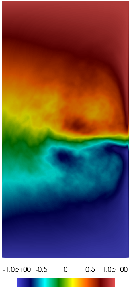
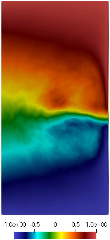
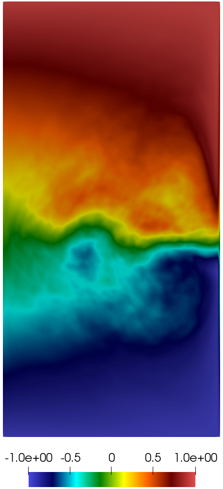
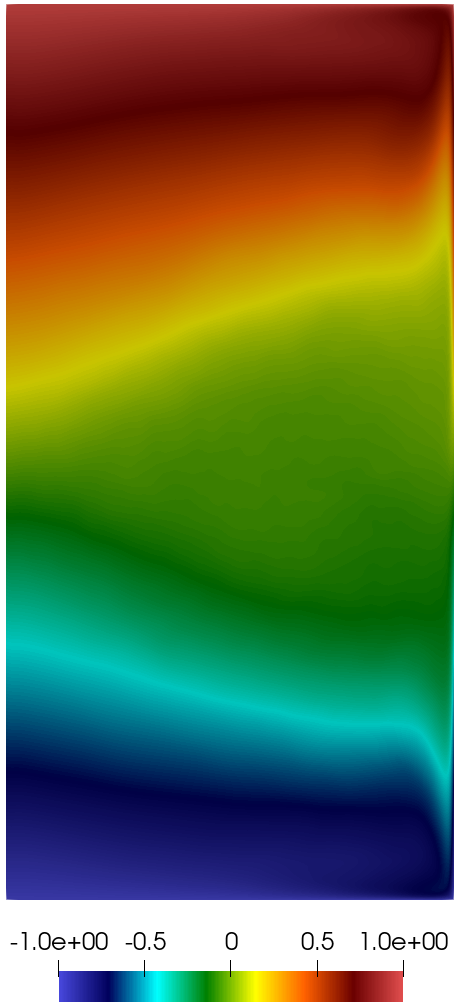
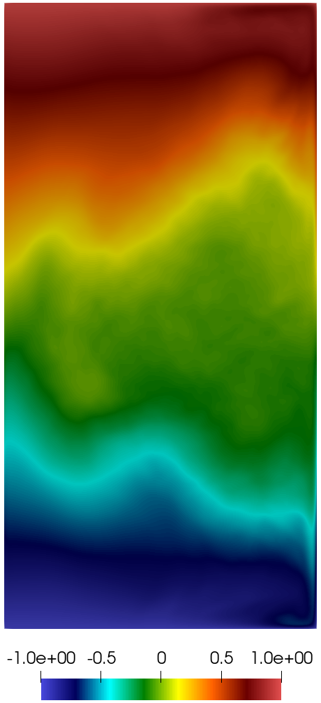
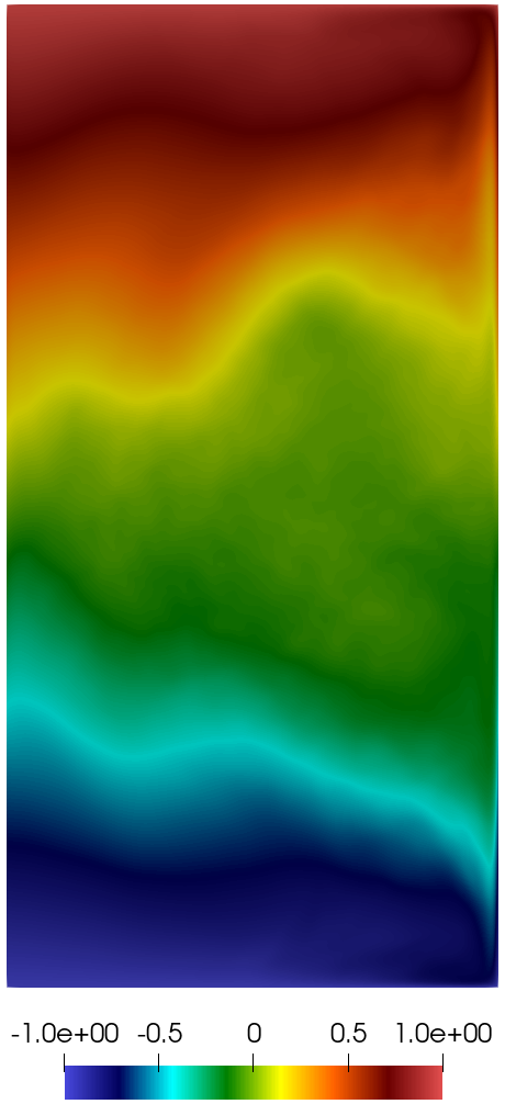
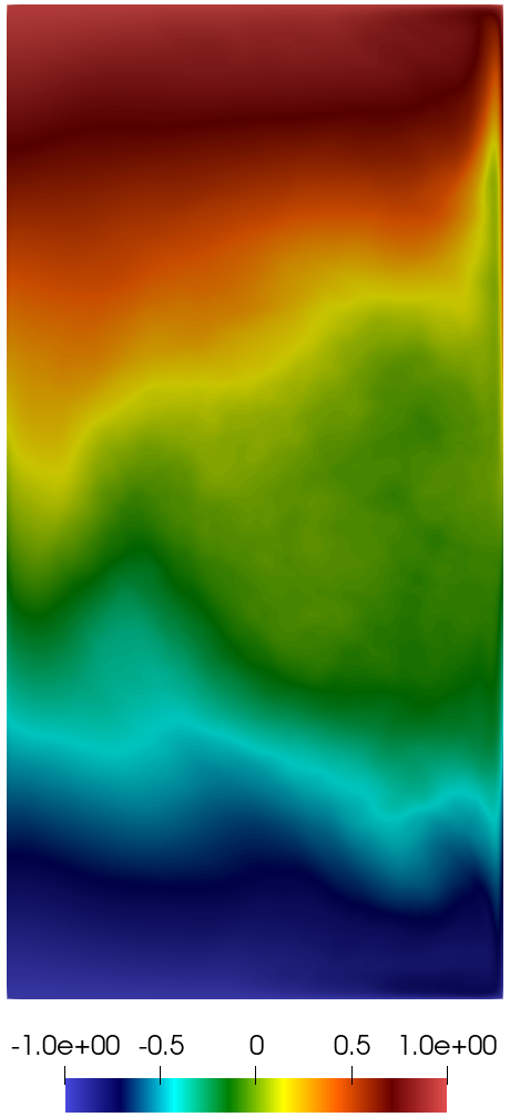
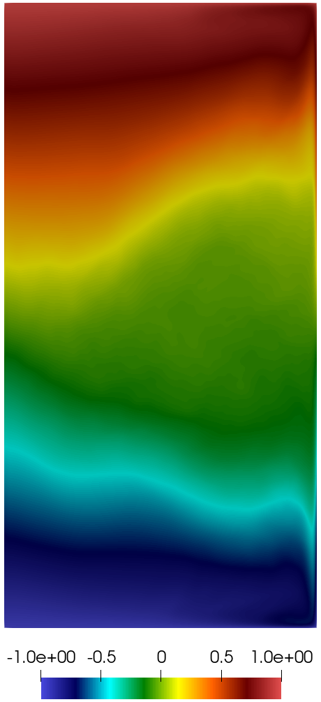
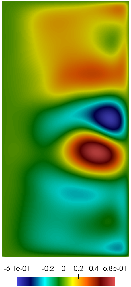
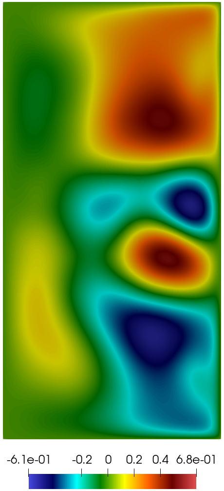
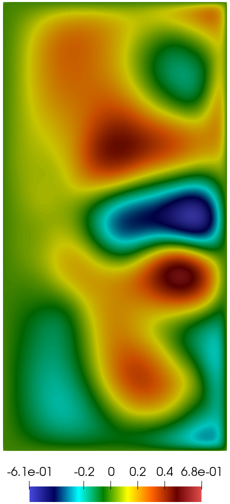
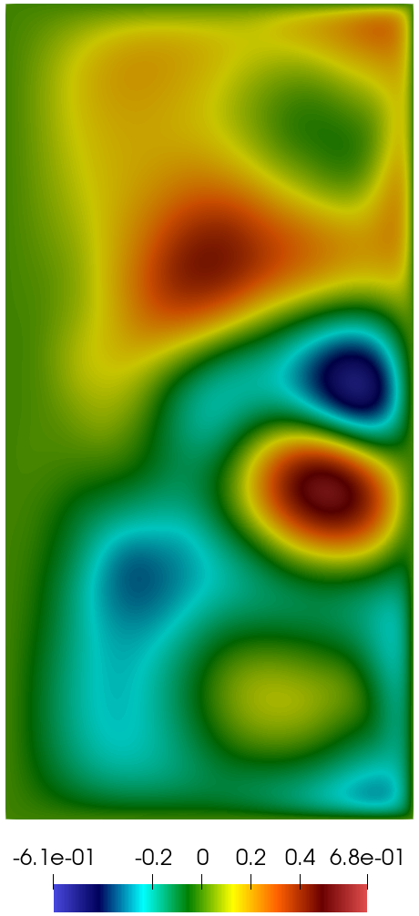
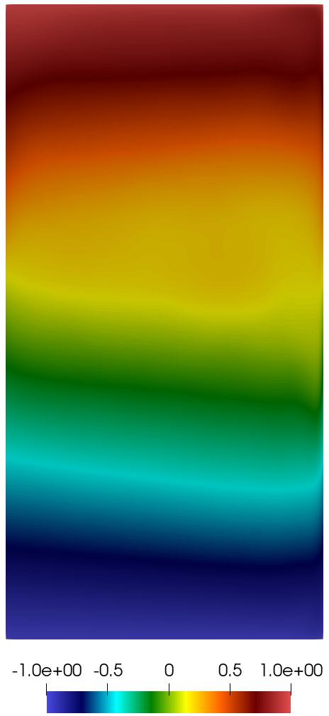
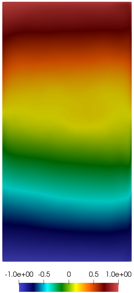
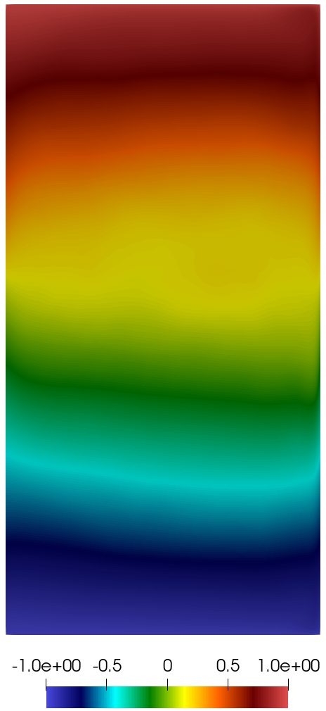
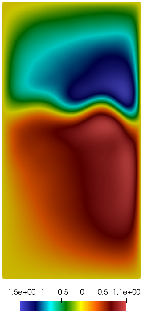
Data-driven reduced order modeling of a two-layer quasi-geostrophic ocean model

Lander Besabe lybesabe@central.uh.edu Michele Girfoglio mgirfogl@sissa.it Annalisa Quaini aquaini@central.uh.edu Gianluigi Rozza grozza@sissa.it SISSA, International School for Advanced Studies, Mathematics Area, mathLab, via Bonomea, Trieste 265 34136, Italy Department of Mathematics, University of Houston, 3551 Cullen Blvd, Houston TX 77204, USA
Abstract

The two-layer quasi-geostrophic equations (2QGE) is a simplified model that describes the dynamics of a stratified, wind-driven ocean in terms of potential vorticity and stream function. Its numerical simulation is plagued by a high computational cost due to the size of the typical computational domain and the need for high resolution to capture the full spectrum of turbulent scales. In this paper, we present a data-driven reduced order model (ROM) for the 2QGE that drastically reduces the computational time to predict ocean dynamics, especially when there are variable physical parameters. The main building blocks of our ROM are: i) proper orthogonal decomposition (POD) and ii) long short-term memory (LSTM) recurrent neural networks. Snapshots data are collected from a high-resolution simulation for part of the time interval of interest and for given parameter values in the case of variable parameters. POD is applied to each field variable to extract the dominant modes and a LSTM model is trained on the modal coefficients associated with the snapshots for each variable. Then, the trained LSTM models predict the modal coefficients for the remaining part of the time interval of interest and for a new parameter value. To illustrate the predictive performance of our POD-LSTM ROM and the corresponding time savings, we consider an extension of the so-called double-gyre wind forcing test. We show that the POD-LSTM ROM is accurate in predicting both time-averaged fields and time-dependent quantities (modal coefficients, enstrophy, and kinetic energy), even when retaining only 10-20% of the singular value energy of the system. The computational speed up for the prediction is about up to 1E+07 compared to a finite volume based full order method.

keywords:
Two-layer quasi-geostrophic equations , Large-scale ocean circulation , Reduced order modeling , Proper orthogonal decomposition , Long short-term memory architecture

1 Introduction

Ocean flows are notorious for being computationally costly to simulate for several reasons, which include the size of the domain (surface area of the order of 1E+06 Km2 and depth of up to 11 Km), the wide spectra of spatial scales, and the need for long time integration to observe long term flow behavior. The spectra of spatial scales depend on the flow regime that is typically characterized by two non-dimensional numbers: the Reynolds number Re𝑅𝑒Re, which is the ratio between the inertial and the viscous forces; and the Rossby number Ro𝑅𝑜Ro, which is the ratio between the inertial force and the Coriolis force. When Re𝑅𝑒Re is large and Ro𝑅𝑜Ro is small, as is typical for ocean flows, the smallest spatial scales are particularly small and thus can only be resolved by extremely fine computational mesh, which are costly.

In order to reduce the computational cost, assumptions are introduced at the modeling level. Since the ocean depth is much smaller than its horizontal length, one can replace the incompressible Navier-Stokes equations with the shallow water equations, which are obtained from the Navier-Stokes equations by averaging on the vertical coordinate. By assuming hydrostatic and geostrophic balance, i.e., very small Ro𝑅𝑜Ro, one can further simplify the shallow water equations to get the single-layer quasi-geostrophic equations (QGE), also known as the barotropic vorticity equations. While the QGE are a widely used model for ocean dynamics, they do not take into account the fact that the ocean is a stratified fluid due to differences in temperature and salinity which result into varying densities. Thus, a slightly more realistic model comes from adding the effect of stratification, which leads to the two-layer quasi-geostrophic equations (2QGE). We note that, although the 2QGE is a simplified model of the ocean, it is still rather complex and computationally expensive when Re𝑅𝑒Re grows large and Ro𝑅𝑜Ro grows small.

When the flow depends on parameters (e.g., Re𝑅𝑒Re, Ro𝑅𝑜Ro, layers depths) known to vary in a given range, as is the case for ocean flows, reduced order modeling (ROM) can be applied to radically reduce the computational time. In broad terms, ROMs are inexpensive surrogates for expensive models. The surrogate is constructed by extracting the dominant system dynamics from selected high-resolution simulations using, e.g., Proper Orthogonal Decomposition (POD) [1, 2]. This computationally intensive initial phase, called offline, is performed once and for all. The expense incurred in this construction process is then amortized over many surrogate solutions. In this second phase, called online, the cheap surrogate solutions can be computed in different ways, e.g., projection methods (e.g., [3]), interpolation (e.g., [4]), or machine learning techniques (e.g., [5]). If projection methods are applied, the ROM is called intrusive, otherwise it is called non-intrusive. ROMs are widely used in many query contexts in fields ranging ranging from structural mechanics [6, 7, 8, 9] to biomedical [10, 11, 12, 13, 14, 15] and naval engineering [16, 17, 18, 19]. See, e.g., [20, 21, 22, 23, 24, 25, 26] for reviews on ROM.

Much interesting work has been done on the construction of intrusive and non-intrusive ROMs for the single-layer QGE. One of the earliest works on this topic [27] constructs a ROM for the QGE using POD to generate the reduced space for vorticity and Galerkin projection for the online phase. Large eddy simulation inspired closure models are utilized to stabilize this projection-based ROM. In [28], two methodologies to capture the unresolved modes (i.e., the modes discarded during the offline phase) are introduced, both based on data-driven corrections. It is shown that these corrections significantly improve the accuracy of the standard POD-Galerkin projection ROM. A hybrid ROM approach for the QGE that uses a convex combination of Galerkin projection and extreme learning machine models is introduced in [29]. In [30] a non-intrusive ROM is constructed by using short-term memory-based (LSTM) architecture trained on the modal coefficients of the high-resolution simulations performed offline. A similar approach to [30], but with LSTM replaced with dynamic mode decomposition [31], is explored in [32]. The only work that applied ROM to a 2QGE model, specifically the stochastic 2QGE, is [33], which levereges a truncated spectral expansion of the baroclinic-barotropic components of the 2QGE for the analysis of the statistical response of the model with respect to important physical quantities.

In this paper, we develop a non-intrusive (also called data-driven) ROM for the 2QGE that uses POD for the generation of a basis for the reduced order space in the offline phase and a simple LSTM architecture to find the coefficients for the reduced basis functions to obtain the ROM approximation of each variable in the online phase. Our approach could be seen as an extension of the methodology in [30] to the 2QGE. However, unlike [30], where POD is applied only to the snapshots matrix for the vorticity, we apply POD to generate different bases for vorticity and stream function. We show that this leads to improved accuracy. For a classical benchmark that displays a very large range of fluctuating spatial and temporal scales, we show that our ROM is not only accurate but extremely efficient, with up to 1E+07 speed up factor in the predictive phase.

The rest of the paper is organized as follows. Sec. 2 describes the 2QGE model. Sec. 3 presents the time and space discretization of the model and the segregated algorithm used to obtain the high-resolution solutions in the offline phase. Sec. 4 presents the details of our POD-LSTM ROM. Sec. 5 discusses the numerical results obtained for an extension of the double-wind gyre forcing benchmark. Conclusions are outlined in Sec. 6.

2 Governing equations

We consider an ocean composed of two layers, each with uniform depth, density, and temperature. These layers, which are called isopycnals, occupy a two-dimensional fixed spatial domain Ω=[x0,xf]×[L/2,L/2]Ωsubscript𝑥0subscript𝑥𝑓𝐿2𝐿2\Omega=[x_{0},x_{f}]\times[-L/2,L/2]. We will call layer 1 the top layer. We assume that the depths of the layers, H1subscript𝐻1H_{1} and H2subscript𝐻2H_{2}, are much smaller than the meridional length L𝐿L. The 2QGE describe the dynamics of these two layers, under some simplifying assumptions. We refer the reader to, e.g., [34, 35, 36, 37, 38], for a thorough description of such assumptions.

Below, we state the 2QGE in non-dimensional form. For this purpose, we need to introduce some notation. Let y𝑦y be the non-dimensional vertical coordinate in the 2D domain and δ=H1H1+H2𝛿subscript𝐻1subscript𝐻1subscript𝐻2\delta=\frac{H_{1}}{H_{1}+H_{2}} the aspect ratio of the depths of the isopycnal layers. We denote with σ𝜎\sigma the friction coefficient at the bottom of the ocean and with ν𝜈\nu the eddy viscosity coefficient. The 2QGE model linearizes the Coriolis frequency f𝑓f as follows: f=f0+βy𝑓subscript𝑓0𝛽𝑦f=f_{0}+\beta y, where f0subscript𝑓0f_{0} is the local Earth rotation rate at y=0𝑦0y=0, which is the center of the basin, and β𝛽\beta is the gradient of the Coriolis frequency. In the non-dimensionalization process, the Rossby number Ro𝑅𝑜Ro, the Reynolds number Re𝑅𝑒Re, and the Froude number Fr𝐹𝑟Fr appear in the model. They are defined as

Re=ULν,Ro=UβL2,Fr=f02UgβH,formulae-sequence𝑅𝑒𝑈𝐿𝜈formulae-sequence𝑅𝑜𝑈𝛽superscript𝐿2𝐹𝑟superscriptsubscript𝑓02𝑈superscript𝑔𝛽𝐻Re=\frac{UL}{\nu},\quad Ro=\frac{U}{\beta L^{2}},\quad Fr=\frac{f_{0}^{2}U}{g^{\prime}\beta H},

where U𝑈U is the characteristic velocity scale, H=H1+H2𝐻subscript𝐻1subscript𝐻2H=H_{1}+H_{2} is the total ocean depth, g=gΔρ/ρ1superscript𝑔𝑔Δ𝜌subscript𝜌1g^{\prime}=g\Delta\rho/\rho_{1} is the reduced gravity, g𝑔g being the gravitational constant, ΔρΔ𝜌\Delta\rho the density difference between the two layers, and ρ1subscript𝜌1\rho_{1} is the density of the top layer. Finally, let (0,T]0𝑇(0,T] be a time interval of interest. The non-dimensional 2QGE read: find potential vorticities qlsubscript𝑞𝑙q_{l} and stream functions ψlsubscript𝜓𝑙\psi_{l}, for l=1,2𝑙12l=1,2, such that in Ω×(0,T]Ω0𝑇\Omega\times(0,T]:

q1t+((×𝚿1)q1)+FrReδΔ(ψ2ψ1)1ReΔq1=F,subscript𝑞1𝑡subscript𝚿1subscript𝑞1𝐹𝑟𝑅𝑒𝛿Δsubscript𝜓2subscript𝜓11𝑅𝑒Δsubscript𝑞1𝐹\displaystyle\frac{\partial q_{1}}{\partial t}+\nabla\cdot\left(\left(\nabla\times\mbox{\boldmath{$\Psi$}}_{1}\right)q_{1}\right)+\frac{Fr}{Re\leavevmode\nobreak\ \delta}\Delta(\psi_{2}-\psi_{1})-\frac{1}{Re}\Delta q_{1}=F, (1)
q2t+((×𝚿2)q2)+FrRe(1δ)Δ(ψ1ψ2)+σΔψ21ReΔq2=0,subscript𝑞2𝑡subscript𝚿2subscript𝑞2𝐹𝑟𝑅𝑒1𝛿Δsubscript𝜓1subscript𝜓2𝜎Δsubscript𝜓21𝑅𝑒Δsubscript𝑞20\displaystyle\frac{\partial q_{2}}{\partial t}+\nabla\cdot\left(\left(\nabla\times\mbox{\boldmath{$\Psi$}}_{2}\right)q_{2}\right)+\frac{Fr}{Re\leavevmode\nobreak\ (1-\delta)}\Delta(\psi_{1}-\psi_{2})+\sigma\Delta\psi_{2}-\frac{1}{Re}\Delta q_{2}=0, (2)
q1=RoΔψ1+y+Frδ(ψ2ψ1),subscript𝑞1𝑅𝑜Δsubscript𝜓1𝑦𝐹𝑟𝛿subscript𝜓2subscript𝜓1\displaystyle q_{1}=Ro\Delta\psi_{1}+y+\frac{Fr}{\delta}\left(\psi_{2}-\psi_{1}\right), (3)
q2=RoΔψ2+y+Fr1δ(ψ1ψ2),subscript𝑞2𝑅𝑜Δsubscript𝜓2𝑦𝐹𝑟1𝛿subscript𝜓1subscript𝜓2\displaystyle q_{2}=Ro\Delta\psi_{2}+y+\frac{Fr}{1-\delta}\left(\psi_{1}-\psi_{2}\right), (4)

where 𝚿l=(0,0,ψl)subscript𝚿𝑙00subscript𝜓𝑙\mbox{\boldmath{$\Psi$}}_{l}=(0,0,\psi_{l}) and F𝐹F is forcing coming from the wind. More details on this model can be found in, e.g., [39, 40, 41, 42, 43, 44].

Following [40], we prescribe free-slip and impenetrable boundary conditions and start the system from a rest state, i.e., we impose the following boundary and initial conditions:

ψl=0,subscript𝜓𝑙0\displaystyle\psi_{l}=0, on Ω×(0,T),on Ω0𝑇\displaystyle\quad\mbox{on }\partial\Omega\times(0,T), (5)
ql=y,subscript𝑞𝑙𝑦\displaystyle q_{l}=y, on Ω×(0,T),on Ω0𝑇\displaystyle\quad\mbox{on }\partial\Omega\times(0,T), (6)
ql(x,y)=ql0=y,subscript𝑞𝑙𝑥𝑦superscriptsubscript𝑞𝑙0𝑦\displaystyle q_{l}(x,y)=q_{l}^{0}=y, in Ω×{0},in Ω0\displaystyle\quad\mbox{in }\Omega\times\{0\}, (7)

for l=1,2𝑙12l=1,2.

3 Full Order Method

Let us start with the time discretization of problem (1)-(4). Let Δt=T/NΔ𝑡𝑇𝑁\Delta t={T}/{N}, where N𝑁N\in\mathbb{N}, tn=t0+nΔtsubscript𝑡𝑛subscript𝑡0𝑛Δ𝑡t_{n}=t_{0}+n\Delta t, for n=1,,N𝑛1𝑁n=1,\dots,N, and denote by fnsuperscript𝑓𝑛f^{n} the approximation of the quantity f𝑓f at time tnsubscript𝑡𝑛t_{n}. Using Backward Difference Formula of order 1, the time-discrete problem reads: given the initial condition ql0=ql(t0)superscriptsubscript𝑞𝑙0subscript𝑞𝑙subscript𝑡0q_{l}^{0}=q_{l}(t_{0}), solve for (qln+1,ψln+1)superscriptsubscript𝑞𝑙𝑛1superscriptsubscript𝜓𝑙𝑛1(q_{l}^{n+1},\psi_{l}^{n+1}) for l=1,2𝑙12l=1,2 and n0𝑛0n\geq 0:

1Δtq1n+1+((×𝚿1n)q1n+1)+FrReδΔ(ψ2n+1ψ1n+1)1ReΔq1n+1=b1n+1,1Δ𝑡superscriptsubscript𝑞1𝑛1superscriptsubscript𝚿1𝑛superscriptsubscript𝑞1𝑛1𝐹𝑟𝑅𝑒𝛿Δsuperscriptsubscript𝜓2𝑛1superscriptsubscript𝜓1𝑛11𝑅𝑒Δsuperscriptsubscript𝑞1𝑛1superscriptsubscript𝑏1𝑛1\displaystyle\frac{1}{\Delta t}q_{1}^{n+1}+\nabla\cdot\left(\left(\nabla\times\mbox{\boldmath{$\Psi$}}_{1}^{n}\right)q_{1}^{n+1}\right)+\frac{Fr}{Re\leavevmode\nobreak\ \delta}\Delta\left(\psi_{2}^{n+1}-\psi_{1}^{n+1}\right)-\frac{1}{Re}\Delta q_{1}^{n+1}=b_{1}^{n+1}, (8)
RoΔψ1n+1+y+Frδ(ψ2n+1ψ1n+1)=q1n+1,𝑅𝑜Δsuperscriptsubscript𝜓1𝑛1𝑦𝐹𝑟𝛿superscriptsubscript𝜓2𝑛1superscriptsubscript𝜓1𝑛1superscriptsubscript𝑞1𝑛1\displaystyle Ro\Delta\psi_{1}^{n+1}+y+\frac{Fr}{\delta}\left(\psi_{2}^{n+1}-\psi_{1}^{n+1}\right)=q_{1}^{n+1}, (9)
1Δtq2n+1+((×𝚿2n)q2n+1)+FrRe(1δ)Δ(ψ1n+1ψ2n+1)1ReΔq2n+1,1Δ𝑡superscriptsubscript𝑞2𝑛1superscriptsubscript𝚿2𝑛superscriptsubscript𝑞2𝑛1𝐹𝑟𝑅𝑒1𝛿Δsuperscriptsubscript𝜓1𝑛1superscriptsubscript𝜓2𝑛11𝑅𝑒Δsuperscriptsubscript𝑞2𝑛1\displaystyle\frac{1}{\Delta t}q_{2}^{n+1}+\nabla\cdot\left(\left(\nabla\times\mbox{\boldmath{$\Psi$}}_{2}^{n}\right)q_{2}^{n+1}\right)+\frac{Fr}{Re\leavevmode\nobreak\ (1-\delta)}\Delta\left(\psi_{1}^{n+1}-\psi_{2}^{n+1}\right)-\frac{1}{Re}\Delta q_{2}^{n+1},
+σΔψ2n+1=b2n+1𝜎Δsuperscriptsubscript𝜓2𝑛1superscriptsubscript𝑏2𝑛1\displaystyle\quad+\sigma\Delta\psi_{2}^{n+1}=b_{2}^{n+1} (10)
RoΔψ2n+1+y+Fr1δ(ψ1n+1ψ2n+1)=q2n+1,𝑅𝑜Δsuperscriptsubscript𝜓2𝑛1𝑦𝐹𝑟1𝛿superscriptsubscript𝜓1𝑛1superscriptsubscript𝜓2𝑛1superscriptsubscript𝑞2𝑛1\displaystyle Ro\Delta\psi_{2}^{n+1}+y+\frac{Fr}{1-\delta}\left(\psi_{1}^{n+1}-\psi_{2}^{n+1}\right)=q_{2}^{n+1}, (11)

where b1n+1=F+q1n/Δtsuperscriptsubscript𝑏1𝑛1𝐹superscriptsubscript𝑞1𝑛Δ𝑡b_{1}^{n+1}=F+q_{1}^{n}/\Delta t and b2n+1=q2n/Δtsuperscriptsubscript𝑏2𝑛1superscriptsubscript𝑞2𝑛Δ𝑡b_{2}^{n+1}=q_{2}^{n}/\Delta t. Note that we have linearized the convective terms in (8) and (10) with a first-order extrapolation. The choice of the BDF1 scheme for time discretization is out of convenience. Of course, other discretization schemes are possible. See, e.g., [45], where we used the BDF2 scheme for the single layer quasi-geostrophic equations.

To contain the computational cost, we adopt a segregated algorithm to solve problem (8)-(11). The algorithm is as follows: given (qln,ψln)superscriptsubscript𝑞𝑙𝑛superscriptsubscript𝜓𝑙𝑛(q_{l}^{n},\psi_{l}^{n}), at time tn+1subscript𝑡𝑛1t_{n+1} perform the following steps:

  • -

    Step 1: find the potential vorticity of the top layer q1n+1superscriptsubscript𝑞1𝑛1q_{1}^{n+1} such that

    1Δtq1n+1+((×𝚿1n)q1n+1)1ReΔq1n+1=b1n+1FrReδΔ(ψ2nψ1n).1Δ𝑡superscriptsubscript𝑞1𝑛1superscriptsubscript𝚿1𝑛superscriptsubscript𝑞1𝑛11𝑅𝑒Δsuperscriptsubscript𝑞1𝑛1superscriptsubscript𝑏1𝑛1𝐹𝑟𝑅𝑒𝛿Δsuperscriptsubscript𝜓2𝑛superscriptsubscript𝜓1𝑛\displaystyle\frac{1}{\Delta t}q_{1}^{n+1}+\nabla\cdot\left(\left(\nabla\times\mbox{\boldmath{$\Psi$}}_{1}^{n}\right)q_{1}^{n+1}\right)-\frac{1}{Re}\Delta q_{1}^{n+1}=b_{1}^{n+1}-\frac{Fr}{Re\leavevmode\nobreak\ \delta}\Delta\left(\psi_{2}^{n}-\psi_{1}^{n}\right). (12)
  • -

    Step 2: find the stream function of the top layer ψ1n+1superscriptsubscript𝜓1𝑛1\psi_{1}^{n+1} such that:

    RoΔψ1n+1+yFrδψ1n+1=q1n+1Frδψ2n.𝑅𝑜Δsuperscriptsubscript𝜓1𝑛1𝑦𝐹𝑟𝛿superscriptsubscript𝜓1𝑛1superscriptsubscript𝑞1𝑛1𝐹𝑟𝛿superscriptsubscript𝜓2𝑛Ro\Delta\psi_{1}^{n+1}+y-\frac{Fr}{\delta}\psi_{1}^{n+1}=q_{1}^{n+1}-\frac{Fr}{\delta}\psi_{2}^{n}. (13)
  • -

    Step 3: find the potential vorticity of the bottom layer q2n+1superscriptsubscript𝑞2𝑛1q_{2}^{n+1} such that:

    1Δtq2n+1+((×𝚿2n)q2n+1)1ReΔq2n+1=b2n+1σΔψ2n1Δ𝑡superscriptsubscript𝑞2𝑛1superscriptsubscript𝚿2𝑛superscriptsubscript𝑞2𝑛11𝑅𝑒Δsuperscriptsubscript𝑞2𝑛1superscriptsubscript𝑏2𝑛1𝜎Δsuperscriptsubscript𝜓2𝑛\displaystyle\frac{1}{\Delta t}q_{2}^{n+1}+\nabla\cdot\left(\left(\nabla\times\mbox{\boldmath{$\Psi$}}_{2}^{n}\right)q_{2}^{n+1}\right)-\frac{1}{Re}\Delta q_{2}^{n+1}=b_{2}^{n+1}-\sigma\Delta\psi_{2}^{n}
    FrRe(1δ)Δ(ψ1n+1ψ2n).𝐹𝑟𝑅𝑒1𝛿Δsuperscriptsubscript𝜓1𝑛1superscriptsubscript𝜓2𝑛\displaystyle\quad-\frac{Fr}{Re\leavevmode\nobreak\ (1-\delta)}\Delta\left(\psi_{1}^{n+1}-\psi_{2}^{n}\right). (14)
  • -

    Step 4: find the stream function of the bottom layer ψ2n+1superscriptsubscript𝜓2𝑛1\psi_{2}^{n+1} such that:

    RoΔψ2n+1+yFr1δψ2n+1=q2n+1Fr1δψ1n+1.𝑅𝑜Δsuperscriptsubscript𝜓2𝑛1𝑦𝐹𝑟1𝛿superscriptsubscript𝜓2𝑛1superscriptsubscript𝑞2𝑛1𝐹𝑟1𝛿superscriptsubscript𝜓1𝑛1Ro\Delta\psi_{2}^{n+1}+y-\frac{Fr}{1-\delta}\psi_{2}^{n+1}=q_{2}^{n+1}-\frac{Fr}{1-\delta}\psi_{1}^{n+1}. (15)

The advantage of this algorithm is that it decouples the computation of each variable.

For the space discretization of eq. (12)–(15), we adopt a Finite Volume (FV) discretization. To begin, we partition the computational domain ΩΩ\Omega into NCsubscript𝑁𝐶N_{C} control volumes with Ωi,i=1,,NCformulae-sequencesubscriptΩ𝑖𝑖1subscript𝑁𝐶\Omega_{i},i=1,\dots,N_{C}, such that iΩi=Ωsubscript𝑖subscriptΩ𝑖Ω\bigcup_{i}\Omega_{i}=\Omega and ΩiΩj=subscriptΩ𝑖subscriptΩ𝑗\Omega_{i}\cap\Omega_{j}=\emptyset for all ij𝑖𝑗i\neq j. Let AjsubscriptA𝑗\textbf{A}_{j} denote the surface vector of each face of the control volume, i.e., the surface area of the face multiplied by the outward normal. The FV approximation is obtained by integrating the 2QGE in space and applying the Gauss divergence theorem:

1Δtq1,kn+1+jϕ1,jnq1,kn+1,j1Rej(q1,kn+1)jAj=b1,kn+1FrReδj((ψ2,knψ1,kn))jAj1Δ𝑡superscriptsubscript𝑞1𝑘𝑛1subscript𝑗superscriptsubscriptitalic-ϕ1𝑗𝑛superscriptsubscript𝑞1𝑘𝑛1𝑗1𝑅𝑒subscript𝑗subscriptsuperscriptsubscript𝑞1𝑘𝑛1𝑗subscriptA𝑗superscriptsubscript𝑏1𝑘𝑛1𝐹𝑟𝑅𝑒𝛿subscript𝑗subscriptsuperscriptsubscript𝜓2𝑘𝑛superscriptsubscript𝜓1𝑘𝑛𝑗subscriptA𝑗\displaystyle\frac{1}{\Delta t}q_{1,k}^{n+1}+\sum_{j}\phi_{1,j}^{n}q_{1,k}^{n+1,j}-\frac{1}{Re}\sum_{j}\left(\nabla q_{1,k}^{n+1}\right)_{j}\cdot\textbf{A}_{j}=b_{1,k}^{n+1}-\frac{Fr}{Re\leavevmode\nobreak\ \delta}\sum_{j}\left(\nabla(\psi_{2,k}^{n}-\psi_{1,k}^{n})\right)_{j}\cdot\textbf{A}_{j} (16)
Roj(ψ1,kn+1)jAj+yk+Frδ(ψ2,knψ1,kn+1)=q1,kn+1,𝑅𝑜subscript𝑗subscriptsuperscriptsubscript𝜓1𝑘𝑛1𝑗subscriptA𝑗subscript𝑦𝑘𝐹𝑟𝛿superscriptsubscript𝜓2𝑘𝑛superscriptsubscript𝜓1𝑘𝑛1superscriptsubscript𝑞1𝑘𝑛1\displaystyle Ro\sum_{j}\left(\nabla\psi_{1,k}^{n+1}\right)_{j}\cdot\textbf{A}_{j}+y_{k}+\frac{Fr}{\delta}\left(\psi_{2,k}^{n}-\psi_{1,k}^{n+1}\right)=q_{1,k}^{n+1}, (17)
1Δtq2,kn+1+jϕ2,jnq2,kn+1,j1Rej(q2,kn+1)jAj=b2,kn+11Δ𝑡superscriptsubscript𝑞2𝑘𝑛1subscript𝑗superscriptsubscriptitalic-ϕ2𝑗𝑛superscriptsubscript𝑞2𝑘𝑛1𝑗1𝑅𝑒subscript𝑗subscriptsuperscriptsubscript𝑞2𝑘𝑛1𝑗subscriptA𝑗superscriptsubscript𝑏2𝑘𝑛1\displaystyle\frac{1}{\Delta t}q_{2,k}^{n+1}+\sum_{j}\phi_{2,j}^{n}q_{2,k}^{n+1,j}-\frac{1}{Re}\sum_{j}\left(\nabla q_{2,k}^{n+1}\right)_{j}\cdot\textbf{A}_{j}=b_{2,k}^{n+1}
+(FrRe(1δ)σ)j(ψ2,kn)jAjFrRe(1δ)j(ψ1,kn+1)jAj,𝐹𝑟𝑅𝑒1𝛿𝜎subscript𝑗subscriptsuperscriptsubscript𝜓2𝑘𝑛𝑗subscriptA𝑗𝐹𝑟𝑅𝑒1𝛿subscript𝑗subscriptsuperscriptsubscript𝜓1𝑘𝑛1𝑗subscriptA𝑗\displaystyle\quad+\left(\frac{Fr}{Re\leavevmode\nobreak\ (1-\delta)}-\sigma\right)\sum_{j}(\nabla\psi_{2,k}^{n})_{j}\cdot\textbf{A}_{j}-\frac{Fr}{Re\leavevmode\nobreak\ (1-\delta)}\sum_{j}\left(\nabla\psi_{1,k}^{n+1}\right)_{j}\cdot\textbf{A}_{j}, (18)
Roj(ψ2,kn+1)jAj+ykFr1δψ2,kn+1=q2,kn+1Fr1δψ1,kn+1,𝑅𝑜subscript𝑗subscriptsuperscriptsubscript𝜓2𝑘𝑛1𝑗subscriptA𝑗subscript𝑦𝑘𝐹𝑟1𝛿superscriptsubscript𝜓2𝑘𝑛1superscriptsubscript𝑞2𝑘𝑛1𝐹𝑟1𝛿superscriptsubscript𝜓1𝑘𝑛1\displaystyle Ro\sum_{j}\left(\nabla\psi_{2,k}^{n+1}\right)_{j}\cdot\textbf{A}_{j}+y_{k}-\frac{Fr}{1-\delta}\psi_{2,k}^{n+1}=q_{2,k}^{n+1}-\frac{Fr}{1-\delta}\psi_{1,k}^{n+1}, (19)

where ql,ksubscript𝑞𝑙𝑘q_{l,k} and ψl,ksubscript𝜓𝑙𝑘\psi_{l,k} are the average potential vorticity and average stream function of layer l𝑙l over the control volume ΩksubscriptΩ𝑘\Omega_{k}, ql,kjsuperscriptsubscript𝑞𝑙𝑘𝑗q_{l,k}^{j} is the potential vorticity associated to the centroid of the j𝑗j-th face and normalized by the volume of ΩksubscriptΩ𝑘\Omega_{k}, bl,ksubscript𝑏𝑙𝑘b_{l,k} is the average discrete forcing, and yksubscript𝑦𝑘y_{k} is the vertical coordinate of the centroid of the control volume ΩksubscriptΩ𝑘\Omega_{k}. For the discretization of the convective terms in (16) and (18), we have introduced:

ϕl,j=(×𝚿l,j)Aj with 𝚿l,j=(0,0,ψl,j)T,subscriptitalic-ϕ𝑙𝑗subscript𝚿𝑙𝑗subscriptA𝑗subscript with 𝚿𝑙𝑗superscript00subscript𝜓𝑙𝑗𝑇\phi_{l,j}=\left(\nabla\times\mbox{\boldmath{$\Psi$}}_{l,j}\right)\cdot\textbf{A}_{j}\text{ with }\mbox{\boldmath{$\Psi$}}_{l,j}=(0,0,\psi_{l,j})^{T}, (20)

which is calculated through a linear interpolation over neighboring cells using a central difference scheme which is of second-order. Also the diffusive terms are approximated using a second order central differencing scheme. For further information on the numerical scheme, we refer the reader to [46, 47].

It was shown in [39] that the numerical scheme presented in this section yields stable and accurate numerical solutions if the mesh is fine enough, i.e., mesh size h<δMsubscript𝛿𝑀h<\delta_{M} where δMsubscript𝛿𝑀\delta_{M} is the Munk scale defined as:

δM=LRoRe3.subscript𝛿𝑀𝐿3𝑅𝑜𝑅𝑒\displaystyle\delta_{M}=L\,\sqrt[3]{\dfrac{Ro}{Re}}. (21)

If one wishes to attain a stable solution with a coarse mesh, i.e., with size h>δMsubscript𝛿𝑀h>\delta_{M}, additional artificial dissipation needs to be introduced in the the system as shown in, e.g., [40, 39].

Lastly, we note that all numerical simulations are executed using GEA [48, 49], an open-source software package which is built upon C++ finite volume library OpenFOAM® [50].

4 Reduced Order Model

This section discusses the main building blocks of our data-driven reduced order model for the 2QGE: proper orthogonal decomposition (POD) and the long short-term memory (LSTM) architecture.

Let us consider first the case where time is the only parameter. We assume that the solution (ql,ψl),l=1,2formulae-sequencesubscript𝑞𝑙subscript𝜓𝑙𝑙12(q_{l},\psi_{l}),l=1,2, of the system (1)–(4) can be written as follows

ql(t,𝒙)qlr(t,𝒙)subscript𝑞𝑙𝑡𝒙superscriptsubscript𝑞𝑙𝑟𝑡𝒙\displaystyle q_{l}(t,\boldsymbol{x})\approx q_{l}^{r}(t,\boldsymbol{x}) =q~l(𝒙)+i=1Nqlrαl,i(t)φl,i(𝒙),absentsubscript~𝑞𝑙𝒙superscriptsubscript𝑖1superscriptsubscript𝑁subscript𝑞𝑙𝑟subscript𝛼𝑙𝑖𝑡subscript𝜑𝑙𝑖𝒙\displaystyle=\widetilde{q}_{l}(\boldsymbol{x})+\sum_{i=1}^{N_{q_{l}}^{r}}\alpha_{l,i}(t)\varphi_{l,i}(\boldsymbol{x}), (22)
ψl(t,𝒙)ψlr(t,𝒙)subscript𝜓𝑙𝑡𝒙superscriptsubscript𝜓𝑙𝑟𝑡𝒙\displaystyle\psi_{l}(t,\boldsymbol{x})\approx\psi_{l}^{r}(t,\boldsymbol{x}) =ψ~l(𝒙)+i=1Nψlrβl,i(t)ξl,i(𝒙),absentsubscript~𝜓𝑙𝒙superscriptsubscript𝑖1superscriptsubscript𝑁subscript𝜓𝑙𝑟subscript𝛽𝑙𝑖𝑡subscript𝜉𝑙𝑖𝒙\displaystyle=\widetilde{\psi}_{l}(\boldsymbol{x})+\sum_{i=1}^{N_{\psi_{l}}^{r}}\beta_{l,i}(t)\xi_{l,i}(\boldsymbol{x}), (23)

where qlrsuperscriptsubscript𝑞𝑙𝑟q_{l}^{r} and ψlrsuperscriptsubscript𝜓𝑙𝑟\psi_{l}^{r} are the reduced order approximations and q~lsubscript~𝑞𝑙\widetilde{q}_{l} and ψ~lsubscript~𝜓𝑙\widetilde{\psi}_{l} are the time-averaged potential vorticity and stream function for each layer computed by

q~l(𝒙)=1Ntp=1Ntql(tp,𝒙),ψ~l(𝒙)=1Ntp=1Ntψl(tp,𝒙).formulae-sequencesubscript~𝑞𝑙𝒙1superscript𝑁𝑡superscriptsubscript𝑝1superscript𝑁𝑡subscript𝑞𝑙subscript𝑡𝑝𝒙subscript~𝜓𝑙𝒙1superscript𝑁𝑡superscriptsubscript𝑝1superscript𝑁𝑡subscript𝜓𝑙subscript𝑡𝑝𝒙\widetilde{q}_{l}(\boldsymbol{x})=\frac{1}{N^{t}}\sum_{p=1}^{N^{t}}q_{l}(t_{p},\boldsymbol{x}),\quad\widetilde{\psi}_{l}(\boldsymbol{x})=\frac{1}{N^{t}}\sum_{p=1}^{N^{t}}\psi_{l}(t_{p},\boldsymbol{x}). (24)

Next, we consider the case where there are physical parameters of interest (e.g., the aspect ratio δ𝛿\delta, friction coefficient σ𝜎\sigma, etc.) that vary in a given range. Let us collect all such parameters in a vector 𝝁𝝁\mu belonging to parameter space 𝒟𝒟\mathbf{\mathcal{D}}. We assume that, for a given 𝝁𝝁\mu, the solution (ql,ψl),l=1,2formulae-sequencesubscript𝑞𝑙subscript𝜓𝑙𝑙12(q_{l},\psi_{l}),l=1,2, of the system (1)–(4) can be written as follows

ql(t,𝒙,𝝁)qlr(t,𝒙,𝝁)subscript𝑞𝑙𝑡𝒙𝝁superscriptsubscript𝑞𝑙𝑟𝑡𝒙𝝁\displaystyle q_{l}(t,\boldsymbol{x},\mbox{\boldmath{$\mu$}})\approx q_{l}^{r}(t,\boldsymbol{x},\mbox{\boldmath{$\mu$}}) =q~l0(𝒙)+i=1Nqlrαl,i(t,𝝁)φl,i(𝒙),absentsuperscriptsubscript~𝑞𝑙0𝒙superscriptsubscript𝑖1superscriptsubscript𝑁subscript𝑞𝑙𝑟subscript𝛼𝑙𝑖𝑡𝝁subscript𝜑𝑙𝑖𝒙\displaystyle=\widetilde{q}_{l}^{0}(\boldsymbol{x})+\sum_{i=1}^{N_{q_{l}}^{r}}\alpha_{l,i}(t,\mbox{\boldmath{$\mu$}})\varphi_{l,i}(\boldsymbol{x}), (25)
ψl(t,𝒙,𝝁)ψlr(t,𝒙,𝝁)subscript𝜓𝑙𝑡𝒙𝝁superscriptsubscript𝜓𝑙𝑟𝑡𝒙𝝁\displaystyle\psi_{l}(t,\boldsymbol{x},\mbox{\boldmath{$\mu$}})\approx\psi_{l}^{r}(t,\boldsymbol{x},\mbox{\boldmath{$\mu$}}) =ψ~l0(𝒙)+i=1Nψlrβl,i(t,𝝁)ξl,i(𝒙),absentsuperscriptsubscript~𝜓𝑙0𝒙superscriptsubscript𝑖1superscriptsubscript𝑁subscript𝜓𝑙𝑟subscript𝛽𝑙𝑖𝑡𝝁subscript𝜉𝑙𝑖𝒙\displaystyle=\widetilde{\psi}_{l}^{0}(\boldsymbol{x})+\sum_{i=1}^{N_{\psi_{l}}^{r}}\beta_{l,i}(t,\mbox{\boldmath{$\mu$}})\xi_{l,i}(\boldsymbol{x}), (26)

where, again, qlrsuperscriptsubscript𝑞𝑙𝑟q_{l}^{r} and ψlrsuperscriptsubscript𝜓𝑙𝑟\psi_{l}^{r} are the reduced order approximations, while q~l0superscriptsubscript~𝑞𝑙0\widetilde{q}_{l}^{0} and ψ~l0superscriptsubscript~𝜓𝑙0\widetilde{\psi}_{l}^{0} are zero-th order approximations of q~l(𝒙,𝝁)subscript~𝑞𝑙𝒙𝝁\widetilde{q}_{l}(\boldsymbol{x},\mbox{\boldmath{$\mu$}}) and ψ~l(𝒙,𝝁)subscript~𝜓𝑙𝒙𝝁\widetilde{\psi}_{l}(\boldsymbol{x},\mbox{\boldmath{$\mu$}}). See Sec. 4.1 for more details on this.

Sec. 4.1 describes how to find the reduced basis functions φl,isubscript𝜑𝑙𝑖\varphi_{l,i} in (22),(25) and ξl,isubscript𝜉𝑙𝑖\xi_{l,i} in (23), (26), and the cardinalities Nqlrsuperscriptsubscript𝑁subscript𝑞𝑙𝑟N_{q_{l}}^{r} and Nψlrsuperscriptsubscript𝑁subscript𝜓𝑙𝑟N_{\psi_{l}}^{r} of the reduced bases. Sec. 4.2 explains how we find coefficients αl,isubscript𝛼𝑙𝑖\alpha_{l,i} in (22),(25) and βl,isubscript𝛽𝑙𝑖\beta_{l,i} in (23),(26) for any new value of t𝑡t and 𝝁𝝁\mu.

4.1 Construction of the POD bases for the reduced spaces

Let us start again from the case where time is the only parameter. The solutions associated to the sampling of the time interval {tp}p=1Ntsuperscriptsubscriptsubscript𝑡𝑝𝑝1superscript𝑁𝑡\{t_{p}\}_{p=1}^{N^{t}}, also called snapshots, will be used to generate a basis for the reduced spaces via POD. The reader interested in learning about the mathematics, applications, and variations of POD is referred to, e.g., [51, 52, 53, 54, 26]. Below, we describe how we use POD to find the reduced basis functions.

From the snapshots, we compute the fluctuations from the time-averaged fields defined by

ql(tp,𝒙)superscriptsubscript𝑞𝑙subscript𝑡𝑝𝒙\displaystyle q_{l}^{\prime}(t_{p},\boldsymbol{x}) =ql(tp,𝒙)q~l(𝒙),absentsubscript𝑞𝑙subscript𝑡𝑝𝒙subscript~𝑞𝑙𝒙\displaystyle=q_{l}(t_{p},\boldsymbol{x})-\widetilde{q}_{l}(\boldsymbol{x}), (27)
ψl(tp,𝒙)superscriptsubscript𝜓𝑙subscript𝑡𝑝𝒙\displaystyle\psi_{l}^{\prime}(t_{p},\boldsymbol{x}) =ψl(tp,𝒙)ψ~l(𝒙),absentsubscript𝜓𝑙subscript𝑡𝑝𝒙subscript~𝜓𝑙𝒙\displaystyle=\psi_{l}(t_{p},\boldsymbol{x})-\widetilde{\psi}_{l}(\boldsymbol{x}), (28)

for l=1,2𝑙12l=1,2 and p=1,,Nt𝑝1superscript𝑁𝑡p=1,\dots,N^{t}. The time-averaged fields are computed as in (24). Let Nhsubscript𝑁N_{h} be the number of degrees of freedom for the FOM solution. Fluctuations (27) and (28) are collected in snapshot matrices. For Φ{ql,ψl}Φsuperscriptsubscript𝑞𝑙superscriptsubscript𝜓𝑙\Phi\in\{q_{l}^{\prime},\psi_{l}^{\prime}\}, l=1,2𝑙12l=1,2, the snapshot matrix 𝒮ΦNh×Ntsubscript𝒮Φsuperscriptsubscript𝑁superscript𝑁𝑡\mathbf{\mathcal{S}}_{\Phi}\in\mathbb{R}^{N_{h}\times N^{t}} is given by

𝒮Φ=[Φ(t1),,Φ(tNt)].subscript𝒮ΦΦsubscript𝑡1Φsubscript𝑡superscript𝑁𝑡\mathbf{\mathcal{S}}_{\Phi}=\left[\Phi(t_{1}),\dots,\Phi(t_{N^{t}})\right]. (29)

Singular value decomposition (SVD) is applied to matrix 𝒮Φsubscript𝒮Φ\mathbf{\mathcal{S}}_{\Phi} for Φ{ql,ψl}Φsuperscriptsubscript𝑞𝑙superscriptsubscript𝜓𝑙\Phi\in\{q_{l}^{\prime},\psi_{l}^{\prime}\}, l=1,2𝑙12l=1,2:

𝒮Φ=𝒰Φ𝚺Φ𝒱ΦTsubscript𝒮Φsubscript𝒰Φsubscript𝚺Φsuperscriptsubscript𝒱Φ𝑇\mathbf{\mathcal{S}}_{\Phi}=\mathbf{\mathcal{U}}_{\Phi}\mathbf{\mbox{\boldmath{$\Sigma$}}}_{\Phi}\mathbf{\mathcal{V}}_{\Phi}^{T} (30)

where 𝒰ΦNh×Ntsubscript𝒰Φsuperscriptsubscript𝑁superscript𝑁𝑡\mathbf{\mathcal{U}}_{\Phi}\in\mathbb{R}^{N_{h}\times N^{t}} and 𝒱ΦNt×Nhsubscript𝒱Φsuperscriptsuperscript𝑁𝑡subscript𝑁\mathbf{\mathcal{V}}_{\Phi}\in\mathbb{R}^{N^{t}\times N_{h}} are matrices whose columns are the left and right singular vectors of 𝒮Φsubscript𝒮Φ\mathbf{\mathcal{S}}_{\Phi}, respectively, and 𝚺ΦNt×Ntsubscript𝚺Φsuperscriptsuperscript𝑁𝑡superscript𝑁𝑡\mathbf{\mbox{\boldmath{$\Sigma$}}}_{\Phi}\in\mathbb{R}^{N^{t}\times N^{t}} is the diagonal matrix whose diagonal entries are the singular values σΦisuperscriptsubscript𝜎Φ𝑖\sigma_{\Phi}^{i} of 𝒮Φsubscript𝒮Φ\mathbf{\mathcal{S}}_{\Phi} arranged in descending order. The POD basis functions are the first NΦrsuperscriptsubscript𝑁Φ𝑟N_{\Phi}^{r} left singular vectors in 𝒰Φsubscript𝒰Φ\mathbf{\mathcal{U}}_{\Phi}, where NΦrsuperscriptsubscript𝑁Φ𝑟N_{\Phi}^{r} is chosen such that for a user-defined threshold 0<δΦ<10subscript𝛿Φ10<\delta_{\Phi}<1:

i=1NΦrσΦii=1NtσΦiδΦ.superscriptsubscript𝑖1superscriptsubscript𝑁Φ𝑟superscriptsubscript𝜎Φ𝑖superscriptsubscript𝑖1superscript𝑁𝑡superscriptsubscript𝜎Φ𝑖subscript𝛿Φ\frac{\sum_{i=1}^{N_{\Phi}^{r}}\sigma_{\Phi}^{i}}{\sum_{i=1}^{N^{t}}\sigma_{\Phi}^{i}}\geq\delta_{\Phi}. (31)

Eq. (31) means that by selecting the first NΦrsuperscriptsubscript𝑁Φ𝑟N_{\Phi}^{r} POD modes as basis functions we retain a user-defined fraction (δΦsubscript𝛿Φ\delta_{\Phi}) of the singular value energy of the system. We will denote with 𝒰Φ,NΦrsubscript𝒰Φsuperscriptsubscript𝑁Φ𝑟\mathbf{\mathcal{U}}_{\Phi,N_{\Phi}^{r}} the matrix consisting of the first NΦrsuperscriptsubscript𝑁Φ𝑟N_{\Phi}^{r} columns of 𝒰Φsubscript𝒰Φ\mathbf{\mathcal{U}}_{\Phi}. The reduced basis space is the span of the columns of 𝒰Φ,NΦrsubscript𝒰Φsuperscriptsubscript𝑁Φ𝑟\mathbf{\mathcal{U}}_{\Phi,N_{\Phi}^{r}}, which represent the most dominant spatial structures from each field of interest. Obviously, one succeeds in generating a reduced basis if NΦrNtmuch-less-thansuperscriptsubscript𝑁Φ𝑟superscript𝑁𝑡N_{\Phi}^{r}\ll N^{t}, i.e., if with a small number of POD modes one can capture reasonably well the system dynamics.

Now that we have the basis functions, we can use eq. (22)–(23) to approximate the snapshots:

ql(tp,𝒙)qlr(tp,𝒙)subscript𝑞𝑙subscript𝑡𝑝𝒙superscriptsubscript𝑞𝑙𝑟subscript𝑡𝑝𝒙\displaystyle q_{l}(t_{p},\boldsymbol{x})\approx q_{l}^{r}(t_{p},\boldsymbol{x}) =q~l(𝒙)+i=1Nqlrαl,i(tp)φl,i(𝒙),absentsubscript~𝑞𝑙𝒙superscriptsubscript𝑖1superscriptsubscript𝑁subscript𝑞𝑙𝑟subscript𝛼𝑙𝑖subscript𝑡𝑝subscript𝜑𝑙𝑖𝒙\displaystyle=\widetilde{q}_{l}(\boldsymbol{x})+\sum_{i=1}^{N_{q_{l}}^{r}}\alpha_{l,i}(t_{p})\varphi_{l,i}(\boldsymbol{x}), (32)
ψl(tp,𝒙)ψlr(tp,𝒙)subscript𝜓𝑙subscript𝑡𝑝𝒙superscriptsubscript𝜓𝑙𝑟subscript𝑡𝑝𝒙\displaystyle\psi_{l}(t_{p},\boldsymbol{x})\approx\psi_{l}^{r}(t_{p},\boldsymbol{x}) =ψ~l(𝒙)+i=1Nψlrβl,i(tp)ξl,i(𝒙),absentsubscript~𝜓𝑙𝒙superscriptsubscript𝑖1superscriptsubscript𝑁subscript𝜓𝑙𝑟subscript𝛽𝑙𝑖subscript𝑡𝑝subscript𝜉𝑙𝑖𝒙\displaystyle=\widetilde{\psi}_{l}(\boldsymbol{x})+\sum_{i=1}^{N_{\psi_{l}}^{r}}\beta_{l,i}(t_{p})\xi_{l,i}(\boldsymbol{x}), (33)

for l=1,2𝑙12l=1,2 and p=1,,Nt𝑝1superscript𝑁𝑡p=1,\dots,N^{t}, where the coefficients αl,i(tp)subscript𝛼𝑙𝑖subscript𝑡𝑝\alpha_{l,i}(t_{p}) and βl,i(tp)subscript𝛽𝑙𝑖subscript𝑡𝑝\beta_{l,i}(t_{p}) for each time instant tpsubscript𝑡𝑝t_{p} are the entries of p𝑝p-th column of matrix 𝒞Φ=𝒰Φ,NΦrT𝒮ΦNΦr×Ntsubscript𝒞Φsuperscriptsubscript𝒰Φsuperscriptsubscript𝑁Φ𝑟𝑇subscript𝒮Φsuperscriptsuperscriptsubscript𝑁Φ𝑟subscript𝑁𝑡\mathbf{\mathcal{C}}_{\Phi}=\mathbf{\mathcal{U}}_{\Phi,N_{\Phi}^{r}}^{T}\mathbf{\mathcal{S}}_{\Phi}\in\mathbb{R}^{N_{\Phi}^{r}\times N_{t}}.

The next subsection explains how we find coefficients αl,isubscript𝛼𝑙𝑖\alpha_{l,i} and βl,isubscript𝛽𝑙𝑖\beta_{l,i} for times that do not belong to partition {tp}p=1Ntsuperscriptsubscriptsubscript𝑡𝑝𝑝1superscript𝑁𝑡\{t_{p}\}_{p=1}^{N^{t}}.

Remark 4.1.

An alternative to the generation of separate POD bases for vorticities and stream functions is to apply POD only to the snapshot matrices of the vorticities to get basis functions φl,isubscript𝜑𝑙𝑖\varphi_{l,i}. Then, the reduced basis functions for the stream functions are obtained from solving Poisson problems:

Δξl,i=φl,i,Δsubscript𝜉𝑙𝑖subscript𝜑𝑙𝑖\Delta\xi_{l,i}=-\varphi_{l,i}, (34)

for i=1,,Nqlr𝑖1superscriptsubscript𝑁subscript𝑞𝑙𝑟i=1,...,N_{q_{l}}^{r} and l=1,2𝑙12l=1,2. Then, using linearity argument, one only needs to compute the modal coefficients once per time step for the vorticities and use them for the reconstruction and prediction of the stream functions too. This means that eq. (22)-(23) become

ql(t,𝒙)qlr(t,𝒙)subscript𝑞𝑙𝑡𝒙superscriptsubscript𝑞𝑙𝑟𝑡𝒙\displaystyle q_{l}(t,\boldsymbol{x})\approx q_{l}^{r}(t,\boldsymbol{x}) =q~l(𝒙)+i=1Nqlrαl,i(t)φl,i(𝒙),absentsubscript~𝑞𝑙𝒙superscriptsubscript𝑖1superscriptsubscript𝑁subscript𝑞𝑙𝑟subscript𝛼𝑙𝑖𝑡subscript𝜑𝑙𝑖𝒙\displaystyle=\widetilde{q}_{l}(\boldsymbol{x})+\sum_{i=1}^{N_{q_{l}}^{r}}\alpha_{l,i}(t)\varphi_{l,i}(\boldsymbol{x}), (35)
ψl(t,𝒙)ψlr(t,𝒙)subscript𝜓𝑙𝑡𝒙superscriptsubscript𝜓𝑙𝑟𝑡𝒙\displaystyle\psi_{l}(t,\boldsymbol{x})\approx\psi_{l}^{r}(t,\boldsymbol{x}) =ψ~l(𝒙)+i=1Nqlrαl,i(t)ξl,i(𝒙).absentsubscript~𝜓𝑙𝒙superscriptsubscript𝑖1superscriptsubscript𝑁subscript𝑞𝑙𝑟subscript𝛼𝑙𝑖𝑡subscript𝜉𝑙𝑖𝒙\displaystyle=\widetilde{\psi}_{l}(\boldsymbol{x})+\sum_{i=1}^{N_{q_{l}}^{r}}\alpha_{l,i}(t)\xi_{l,i}(\boldsymbol{x}). (36)

This strategy has been used for the single layer quasi-geostrophic equations in [30, 28, 29, 32, 55].

If, in addition to time, there are variable physical parameters 𝝁𝝁\mu, we need to sample 𝒟×(0,T]𝒟0𝑇\mathbf{\mathcal{D}}\times(0,T]. For this, we collect the solutions associated to partition {𝝁k}k=1Nd×{tp}p=1Ntsuperscriptsubscriptsubscript𝝁𝑘𝑘1superscript𝑁𝑑superscriptsubscriptsubscript𝑡𝑝𝑝1superscript𝑁𝑡\{\mbox{\boldmath{$\mu$}}_{k}\}_{k=1}^{N^{d}}\times\{t_{p}\}_{p=1}^{N^{t}} of 𝒟×(0,T]𝒟0𝑇\mathbf{\mathcal{D}}\times(0,T]. From the snapshots, we compute the fluctuations from the time-averaged fields defined by

ql(tp,𝒙,𝝁k)superscriptsubscript𝑞𝑙subscript𝑡𝑝𝒙subscript𝝁𝑘\displaystyle q_{l}^{\prime}(t_{p},\boldsymbol{x},\mbox{\boldmath{$\mu$}}_{k}) =ql(tp,𝒙,𝝁k)q~(𝒙,𝝁k),absentsubscript𝑞𝑙subscript𝑡𝑝𝒙subscript𝝁𝑘~𝑞𝒙subscript𝝁𝑘\displaystyle=q_{l}(t_{p},\boldsymbol{x},\mbox{\boldmath{$\mu$}}_{k})-\widetilde{q}(\boldsymbol{x},\mbox{\boldmath{$\mu$}}_{k}), (37)
ψl(tp,𝒙,𝝁k)superscriptsubscript𝜓𝑙subscript𝑡𝑝𝒙subscript𝝁𝑘\displaystyle\psi_{l}^{\prime}(t_{p},\boldsymbol{x},\mbox{\boldmath{$\mu$}}_{k}) =ψl(tp,𝒙,𝝁k)ψ~(𝒙,𝝁k),absentsubscript𝜓𝑙subscript𝑡𝑝𝒙subscript𝝁𝑘~𝜓𝒙subscript𝝁𝑘\displaystyle=\psi_{l}(t_{p},\boldsymbol{x},\mbox{\boldmath{$\mu$}}_{k})-\widetilde{\psi}(\boldsymbol{x},\mbox{\boldmath{$\mu$}}_{k}), (38)

for l=1,2𝑙12l=1,2, k=1,,Nd𝑘1superscript𝑁𝑑k=1,\dots,N^{d}, and p=1,,Nt𝑝1superscript𝑁𝑡p=1,\dots,N^{t}. Let Ns=Nd×Ntsubscript𝑁𝑠superscript𝑁𝑑superscript𝑁𝑡N_{s}=N^{d}\times N^{t}. Fluctuations (37) and (38) are stored in snapshot matrices 𝒮ΦNh×Nssubscript𝒮Φsuperscriptsubscript𝑁subscript𝑁𝑠\mathbf{\mathcal{S}}_{\Phi}\in\mathbb{R}^{N_{h}\times N_{s}}:

𝒮Φ=[Φ(𝝁1,t1),,Φ(𝝁1,tNt),,Φ(𝝁Nd,tNt)],subscript𝒮ΦΦsubscript𝝁1subscript𝑡1Φsubscript𝝁1subscript𝑡superscript𝑁𝑡Φsubscript𝝁superscript𝑁𝑑subscript𝑡superscript𝑁𝑡\mathbf{\mathcal{S}}_{\Phi}=\left[\Phi(\mbox{\boldmath{$\mu$}}_{1},t_{1}),\dots,\Phi(\mbox{\boldmath{$\mu$}}_{1},t_{N^{t}}),\dots,\Phi(\mbox{\boldmath{$\mu$}}_{N^{d}},t_{N^{t}})\right], (39)

for Φ{ql,ψl}Φsuperscriptsubscript𝑞𝑙superscriptsubscript𝜓𝑙\Phi\in\{q_{l}^{\prime},\psi_{l}^{\prime}\}, l=1,2𝑙12l=1,2. At this point, the procedure is the same as in the case of time as the only parameter, i.e., one applies SVD and retains the first NΦrsuperscriptsubscript𝑁Φ𝑟N_{\Phi}^{r} left singular vectors according to criterion (31) to generate the POD basis. With that, one uses (25)-(26) to approximate the snapshots:

ql(tp,𝒙,𝝁k)qlr(tp,𝒙,𝝁k)subscript𝑞𝑙subscript𝑡𝑝𝒙subscript𝝁𝑘superscriptsubscript𝑞𝑙𝑟subscript𝑡𝑝𝒙subscript𝝁𝑘\displaystyle q_{l}(t_{p},\boldsymbol{x},\mbox{\boldmath{$\mu$}}_{k})\approx q_{l}^{r}(t_{p},\boldsymbol{x},\mbox{\boldmath{$\mu$}}_{k}) =q~l(𝒙,𝝁k)+i=1Nqlrαl,i(tp,𝝁k)φl,i(𝒙),absentsubscript~𝑞𝑙𝒙subscript𝝁𝑘superscriptsubscript𝑖1superscriptsubscript𝑁subscript𝑞𝑙𝑟subscript𝛼𝑙𝑖subscript𝑡𝑝subscript𝝁𝑘subscript𝜑𝑙𝑖𝒙\displaystyle=\widetilde{q}_{l}(\boldsymbol{x},\mbox{\boldmath{$\mu$}}_{k})+\sum_{i=1}^{N_{q_{l}}^{r}}\alpha_{l,i}(t_{p},\mbox{\boldmath{$\mu$}}_{k})\varphi_{l,i}(\boldsymbol{x}), (40)
ψl(tp,𝒙,𝝁k)ψlr(tp,𝒙,𝝁k)subscript𝜓𝑙subscript𝑡𝑝𝒙subscript𝝁𝑘superscriptsubscript𝜓𝑙𝑟subscript𝑡𝑝𝒙subscript𝝁𝑘\displaystyle\psi_{l}(t_{p},\boldsymbol{x},\mbox{\boldmath{$\mu$}}_{k})\approx\psi_{l}^{r}(t_{p},\boldsymbol{x},\mbox{\boldmath{$\mu$}}_{k}) =ψ~l(𝒙,𝝁k)+i=1Nψlrβl,i(tp,𝝁k)ξl,i(𝒙),absentsubscript~𝜓𝑙𝒙subscript𝝁𝑘superscriptsubscript𝑖1superscriptsubscript𝑁subscript𝜓𝑙𝑟subscript𝛽𝑙𝑖subscript𝑡𝑝subscript𝝁𝑘subscript𝜉𝑙𝑖𝒙\displaystyle=\widetilde{\psi}_{l}(\boldsymbol{x},\mbox{\boldmath{$\mu$}}_{k})+\sum_{i=1}^{N_{\psi_{l}}^{r}}\beta_{l,i}(t_{p},\mbox{\boldmath{$\mu$}}_{k})\xi_{l,i}(\boldsymbol{x}), (41)

for l=1,2𝑙12l=1,2, k=1,,Nd𝑘1superscript𝑁𝑑k=1,\dots,N^{d}, and p=1,,Nt𝑝1superscript𝑁𝑡p=1,\dots,N^{t}, where the coefficients αl,i(tp,𝝁k)subscript𝛼𝑙𝑖subscript𝑡𝑝subscript𝝁𝑘\alpha_{l,i}(t_{p},\mbox{\boldmath{$\mu$}}_{k}) and βl,i(tp,𝝁k)subscript𝛽𝑙𝑖subscript𝑡𝑝subscript𝝁𝑘\beta_{l,i}(t_{p},\mbox{\boldmath{$\mu$}}_{k}) for each time instant tpsubscript𝑡𝑝t_{p} and parameter 𝝁ksubscript𝝁𝑘\mbox{\boldmath{$\mu$}}_{k} are computed in the same way as when time is the only parameter.

For a time t𝑡t and parameter 𝝁𝝁\mu not in the sampling set {𝝁k}k=1Nd×{tp}p=1Ntsuperscriptsubscriptsubscript𝝁𝑘𝑘1superscript𝑁𝑑superscriptsubscriptsubscript𝑡𝑝𝑝1superscript𝑁𝑡\{\mbox{\boldmath{$\mu$}}_{k}\}_{k=1}^{N^{d}}\times\{t_{p}\}_{p=1}^{N^{t}}, we need to find q~l0superscriptsubscript~𝑞𝑙0\widetilde{q}_{l}^{0} and ψ~l0superscriptsubscript~𝜓𝑙0\widetilde{\psi}_{l}^{0} in (25)-(26), together with coefficients αl,isubscript𝛼𝑙𝑖\alpha_{l,i} and βl,isubscript𝛽𝑙𝑖\beta_{l,i}. The zero-th order approximations q~l0superscriptsubscript~𝑞𝑙0\widetilde{q}_{l}^{0} and ψ~l0superscriptsubscript~𝜓𝑙0\widetilde{\psi}_{l}^{0} are simply given by

q~l0(𝒙)=1Ntp=1Ntql(tp,𝒙,𝝁c),ψ~l0(𝒙)=1Ntp=1Ntψl(tp,𝒙,𝝁c),formulae-sequencesuperscriptsubscript~𝑞𝑙0𝒙1superscript𝑁𝑡superscriptsubscript𝑝1superscript𝑁𝑡subscript𝑞𝑙subscript𝑡𝑝𝒙subscript𝝁𝑐superscriptsubscript~𝜓𝑙0𝒙1superscript𝑁𝑡superscriptsubscript𝑝1superscript𝑁𝑡subscript𝜓𝑙subscript𝑡𝑝𝒙subscript𝝁𝑐\widetilde{q}_{l}^{0}(\boldsymbol{x})=\frac{1}{N^{t}}\sum_{p=1}^{N^{t}}q_{l}(t_{p},\boldsymbol{x},\mbox{\boldmath{$\mu$}}_{c}),\quad\widetilde{\psi}_{l}^{0}(\boldsymbol{x})=\frac{1}{N^{t}}\sum_{p=1}^{N^{t}}\psi_{l}(t_{p},\boldsymbol{x},\mbox{\boldmath{$\mu$}}_{c}), (42)

where 𝝁csubscript𝝁𝑐\mbox{\boldmath{$\mu$}}_{c} is the sample in {𝝁k}k=1Ndsuperscriptsubscriptsubscript𝝁𝑘𝑘1superscript𝑁𝑑\{\mbox{\boldmath{$\mu$}}_{k}\}_{k=1}^{N^{d}} closest to 𝝁𝝁\mu in the Euclidean norm. How to find coefficients αl,isubscript𝛼𝑙𝑖\alpha_{l,i} and βl,isubscript𝛽𝑙𝑖\beta_{l,i} is explained in the next subsection.

4.2 The data-driven ROM based on LSTM

We develop a data-driven ROM using a deep learning technique [56] that performs well in the prediction of a time-series behavior: a type of recurrent neural network (RNN) called long short-term memory. The LSTM architecture was introduced in [57] to resolve the problem of vanishing or exploding gradients that RNNs often encounter [58]. The main mechanisms of the LSTM architecture are gating activation functions and cell states that serve as the memory of the network. It is thanks to the gating functions that vanishing gradients are avoided, while the fact that the gradient of the cell states is bounded by 111 avoids exploding gradients [59]. Without incurring into gradient problems, the LSTM learns long term behavior better than regular RNNs.

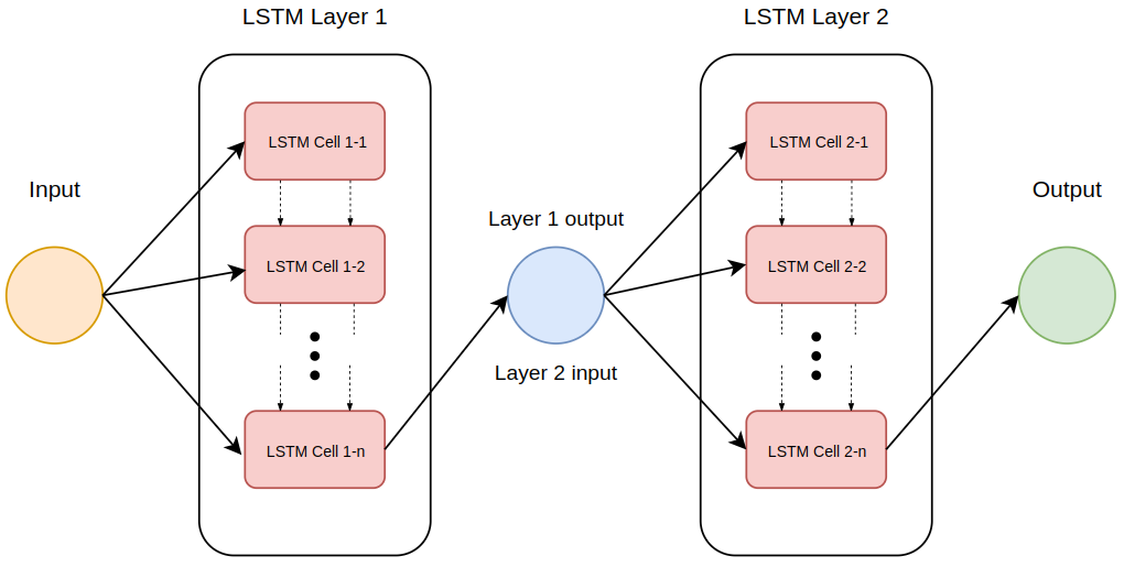
Like any RNN, LSTM contains recurrent layers and neurons. Within these layers, there are memory blocks, also called LSTM cells. An illustration of a LSTM network with two layers and n𝑛n memory blocks in each layer is shown as an example in Fig. 1. Every layer is its own network, which means that if we have two layers the input of the second layer is the output of the first layer, with the option to pass them through an activation function before passing it to the next layer.
Refer to caption
Figure 1: Illustration of an LSTM architecture with 2 layers and n𝑛n cells (or memory blocks) in each layer.

Before explaining how each cell in Fig. 1 works, we specify the input and output of our LSTM network. In order to do that, we need to introduce one important hyperparameter: the lookback window σLsubscript𝜎𝐿\sigma_{L}, which indicates how many steps in the history of the data series the LSTM considers, both in training and prediction. Let us consider the reduced space for the potential vorticity in layer l𝑙l as representative. For simplicity of notation, we denote with N𝑁N the number of retained modes Nqlrsuperscriptsubscript𝑁subscript𝑞𝑙𝑟N_{q_{l}}^{r}. For a given time tpsubscript𝑡𝑝t_{p} and parameter vector 𝝁ksubscript𝝁𝑘\mbox{\boldmath{$\mu$}}_{k}, we store the time information tp,,tpσL+1subscript𝑡𝑝subscript𝑡𝑝subscript𝜎𝐿1t_{p},\dots,t_{p-\sigma_{L}+1}, parameter vector 𝝁ksubscript𝝁𝑘\mbox{\boldmath{$\mu$}}_{k}, and coefficients αl,i(tp)subscript𝛼𝑙𝑖subscript𝑡𝑝\alpha_{l,i}(t_{p}) in (32) in a σL×(N+Nd+1)subscript𝜎𝐿𝑁superscript𝑁𝑑1\sigma_{L}\times(N+N^{d}+1) matrix

[𝝁ktpαl,1(tp)αl,N(tp)𝝁ktpσL+1αl,1(tpσL+1)αl,N(tpσL+1)].delimited-[]subscript𝝁𝑘subscript𝑡𝑝subscript𝛼𝑙1subscript𝑡𝑝subscript𝛼𝑙𝑁subscript𝑡𝑝subscript𝝁𝑘subscript𝑡𝑝subscript𝜎𝐿1subscript𝛼𝑙1subscript𝑡𝑝subscript𝜎𝐿1subscript𝛼𝑙𝑁subscript𝑡𝑝subscript𝜎𝐿1\left[\begin{array}[]{ccccc}\mbox{\boldmath{$\mu$}}_{k}&t_{p}&\alpha_{l,1}(t_{p})&\cdots&\alpha_{l,N}(t_{p})\\ \vdots&\vdots&\vdots&\ddots&\vdots\\ \mbox{\boldmath{$\mu$}}_{k}&t_{p-\sigma_{L}+1}&\alpha_{l,1}(t_{p-\sigma_{L}+1})&\cdots&\alpha_{l,N}(t_{p-\sigma_{L}+1})\end{array}\right]. (43)

Through the LSTM architecture, we aim to match the training matrix (43), i.e., the input at time tpsubscript𝑡𝑝t_{p} and for parameter vector 𝝁ksubscript𝝁𝑘\mbox{\boldmath{$\mu$}}_{k}, to the corresponding output training vector [αl,1(tp+1),,αl,K(tp+1)]subscript𝛼𝑙1subscript𝑡𝑝1subscript𝛼𝑙𝐾subscript𝑡𝑝1\left[\alpha_{l,1}(t_{p+1}),\dots,\alpha_{l,K}(t_{p+1})\right], i.e., the coefficients for the reduced order approximation at time tp+1subscript𝑡𝑝1t_{p+1}. Below, we explain how each cell in Fig. 1 works.

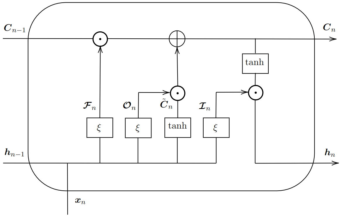
The generic LSTM cell, denoted with n𝑛n, manages the flow of training/testing data by selectively adding information through the input gate 𝓘nsubscript𝓘𝑛\mbox{\boldmath{$\mathbf{\mathcal{I}}$}}_{n}, forgetting some of such data in the forget gate 𝓕nsubscript𝓕𝑛\mbox{\boldmath{$\mathbf{\mathcal{F}}$}}_{n}, and then passing them through the next cell (n+1𝑛1n+1) through the output gate 𝓞nsubscript𝓞𝑛\mbox{\boldmath{$\mathbf{\mathcal{O}}$}}_{n}. For simplicity, let us denote the cell input with 𝒙nsubscript𝒙𝑛\mbox{\boldmath{$x$}}_{n}, which comes from either the input of the network or an intermediate input as shown in Fig. 1. The generic cell n𝑛n takes as input also the output of the preceding cell 𝒉n1subscript𝒉𝑛1\mbox{\boldmath{$h$}}_{n-1}, which can be interpreted as the short term memory of the network. See Fig. 1. Let us denote with [𝒉n1,𝒙n]subscript𝒉𝑛1subscript𝒙𝑛\left[\mbox{\boldmath{$h$}}_{n-1},\mbox{\boldmath{$x$}}_{n}\right] the concatenation of 𝒉n1subscript𝒉𝑛1\mbox{\boldmath{$h$}}_{n-1} and 𝒙nsubscript𝒙𝑛\mbox{\boldmath{$x$}}_{n}. We have

𝓘nsubscript𝓘𝑛\displaystyle\mbox{\boldmath{$\mathbf{\mathcal{I}}$}}_{n} =ξ(WI[𝒉n1,𝒙n]+𝒃I),absent𝜉subscript𝑊𝐼subscript𝒉𝑛1subscript𝒙𝑛subscript𝒃𝐼\displaystyle=\xi\left(W_{I}\left[\mbox{\boldmath{$h$}}_{n-1},\mbox{\boldmath{$x$}}_{n}\right]+\mbox{\boldmath{$b$}}_{I}\right),
𝓕nsubscript𝓕𝑛\displaystyle\mbox{\boldmath{$\mathbf{\mathcal{F}}$}}_{n} =ξ(WF[𝒉n1,𝒙n]+𝒃F),absent𝜉subscript𝑊𝐹subscript𝒉𝑛1subscript𝒙𝑛subscript𝒃𝐹\displaystyle=\xi\left(W_{F}\left[\mbox{\boldmath{$h$}}_{n-1},\mbox{\boldmath{$x$}}_{n}\right]+\mbox{\boldmath{$b$}}_{F}\right),
𝓞nsubscript𝓞𝑛\displaystyle\mbox{\boldmath{$\mathbf{\mathcal{O}}$}}_{n} =ξ(WO[𝒉n1,𝒙n]+𝒃O),absent𝜉subscript𝑊𝑂subscript𝒉𝑛1subscript𝒙𝑛subscript𝒃𝑂\displaystyle=\xi\left(W_{O}\left[\mbox{\boldmath{$h$}}_{n-1},\mbox{\boldmath{$x$}}_{n}\right]+\mbox{\boldmath{$b$}}_{O}\right),

where ξ𝜉\xi is the sigmoid function with range in (0,1)01(0,1), WIsubscript𝑊𝐼W_{I}, WFsubscript𝑊𝐹W_{F}, and WOsubscript𝑊𝑂W_{O} are matrices of weights, while 𝒃Isubscript𝒃𝐼\mbox{\boldmath{$b$}}_{I}, 𝒃Fsubscript𝒃𝐹\mbox{\boldmath{$b$}}_{F}, and 𝒃Osubscript𝒃𝑂\mbox{\boldmath{$b$}}_{O} are vectors of biases. The cell output 𝒉nsubscript𝒉𝑛\mbox{\boldmath{$h$}}_{n} is computed as

𝒉nsubscript𝒉𝑛\displaystyle\mbox{\boldmath{$h$}}_{n} =𝓞ntanh(𝑪n),absentdirect-productsubscript𝓞𝑛subscript𝑪𝑛\displaystyle=\mbox{\boldmath{$\mathbf{\mathcal{O}}$}}_{n}\odot\tanh\left(\mbox{\boldmath{$C$}}_{n}\right),

where direct-product\odot is the Hadamard product and 𝑪nsubscript𝑪𝑛\mbox{\boldmath{$C$}}_{n} is the cell state given by

𝑪nsubscript𝑪𝑛\displaystyle\mbox{\boldmath{$C$}}_{n} =𝓕n𝑪n1+𝓘n𝑪~n,absentdirect-productsubscript𝓕𝑛subscript𝑪𝑛1direct-productsubscript𝓘𝑛subscript~𝑪𝑛\displaystyle=\mbox{\boldmath{$\mathbf{\mathcal{F}}$}}_{n}\odot\mbox{\boldmath{$C$}}_{n-1}+\mbox{\boldmath{$\mathbf{\mathcal{I}}$}}_{n}\odot\widetilde{\mbox{\boldmath{$C$}}}_{n},

with 𝑪~nsubscript~𝑪𝑛\widetilde{\mbox{\boldmath{$C$}}}_{n} representing the updated cell state

𝑪~nsubscript~𝑪𝑛\displaystyle\widetilde{\mbox{\boldmath{$C$}}}_{n} =tanh(WC[𝒉n1,𝒙n]+𝒃C).absentsubscript𝑊𝐶subscript𝒉𝑛1subscript𝒙𝑛subscript𝒃𝐶\displaystyle=\tanh\left(W_{C}\left[\mbox{\boldmath{$h$}}_{n-1},\mbox{\boldmath{$x$}}_{n}\right]+\mbox{\boldmath{$b$}}_{C}\right).

Here, WCsubscript𝑊𝐶W_{C} is a matrix of weights and 𝒃Csubscript𝒃𝐶\mbox{\boldmath{$b$}}_{C} is a vector of biases. The cell state 𝑪nsubscript𝑪𝑛\mbox{\boldmath{$C$}}_{n} flows through the network passing some linear operations and can be seen as the long term memory of the network. See Fig. 2. A schematic diagram of an LSTM cell as described above is shown in Fig. 3. For a detailed discussion on the architecture and mathematics behind LSTM networks, see, e.g., [60].

Refer to caption
Figure 2: Connections among adjacent LSTM cells.
Refer to caption
Figure 3: Schematic diagram of an LSTM cell.

Above, we have explained how the LSTM network for the potential vorticity in layer l𝑙l works. We will call that network qlsubscriptsubscript𝑞𝑙\mathbf{\mathcal{M}}_{q_{l}}, l=1,2𝑙12l=1,2. The LSTM network for the stream function in layer l𝑙l, denoted with ψlsubscriptsubscript𝜓𝑙\mathbf{\mathcal{M}}_{\psi_{l}}, will be built analogously, using the same lookback window σLsubscript𝜎𝐿\sigma_{L}.

5 Numerical Results

To assess the performance of POD-LSTM ROM presented in Sec. 4 in terms of both reconstruction and prediction, we consider an extension [39] of the so-called double-wind gyre forcing experiment, which is a classical benchmark for new numerical models of geophysical flows [61, 62, 63, 64, 65, 45, 66, 27, 67].

The computational domain for this benchmark is Ω=[0,1]×[1,1]Ω0111\Omega=[0,1]\times[-1,1] and the forcing term in (1) is F=sin(πy)𝐹𝜋𝑦F=\sin(\pi y). For the FOM, we use a mesh size h=1/2561256h=1/256 which is about 3 times smaller than the Munk scale for the chosen value of eddy viscosity ν=155𝜈155\nu=155 m2s-1. The time step is set to Δt=2.5E05Δ𝑡2.5E05\Delta t=2.5\mathrm{E}-05. We collect snapshots over time interval [10,50]1050[10,50] every 0.10.10.1 unit of time, i.e., 401 snapshots for each variable (q1,q2,ψ1,superscriptsubscript𝑞1superscriptsubscript𝑞2superscriptsubscript𝜓1q_{1}^{\prime},q_{2}^{\prime},\psi_{1}^{\prime}, and ψ2superscriptsubscript𝜓2\psi_{2}^{\prime}), and build the corresponding POD reduced spaces as explained in Sec. 4.1.

In Sec. 5.1, we fix all the physical parameters, keeping time as the only parameter. Specifically, we set

Ro=0.001, Re=450, Fr=0.1, σ=0.005, and δ=0.5.formulae-sequence𝑅𝑜0.001formulae-sequence 𝑅𝑒450formulae-sequence 𝐹𝑟0.1formulae-sequence 𝜎0.005 and 𝛿0.5Ro=0.001,\text{ }Re=450,\text{ }Fr=0.1,\text{ }\sigma=0.005,\text{ and }\delta=0.5. (44)

With the POD-LSTM ROM, we will reconstruct the time-averaged quantities q~lsubscript~𝑞𝑙\widetilde{q}_{l} and ψ~lsubscript~𝜓𝑙\widetilde{\psi}_{l}, l=1,2𝑙12l=1,2, during the [10,50]1050[10,50] time interval to evaluate its performance in system identification. Additionally, we will use the POD-LSTM ROM to predict the same quantities over (50,100]50100(50,100]. We will also consider two metrics to evaluate the system identification and the prediction:

  • -

    a root mean square error for the field Φ{q1,q2,ψ1,ψ2}Φsubscript𝑞1subscript𝑞2subscript𝜓1subscript𝜓2\Phi\in\{q_{1},q_{2},\psi_{1},\psi_{2}\} [30]:

    εΦ(1)=1NxNyi=1Nxj=1Ny|Φ~i,jFOMΦ~i,jROM|2,superscriptsubscript𝜀Φ11subscript𝑁𝑥subscript𝑁𝑦superscriptsubscript𝑖1subscript𝑁𝑥superscriptsubscript𝑗1𝑁𝑦superscriptsuperscriptsubscript~Φ𝑖𝑗FOMsuperscriptsubscript~Φ𝑖𝑗ROM2\varepsilon_{\Phi}^{(1)}=\sqrt{\frac{1}{N_{x}N_{y}}\sum_{i=1}^{N_{x}}\sum_{j=1}^{Ny}\absolutevalue{\widetilde{\Phi}_{i,j}^{\text{FOM}}-\widetilde{\Phi}_{i,j}^{\text{ROM}}}^{2}}, (45)

    where Nxsubscript𝑁𝑥N_{x} and Nysubscript𝑁𝑦N_{y} are the number of cells in the x𝑥x and y𝑦y directions, respectively, Φ~FOMsuperscript~ΦFOM\widetilde{\Phi}^{\text{FOM}} and Φ~ROMsuperscript~ΦROM\widetilde{\Phi}^{\text{ROM}} are the time-averaged fields ΦΦ\Phi computed by the FOM and POD-LSTM, respectively;

  • -

    the relative L2superscript𝐿2L^{2} error:

    εΦ(2)=Φ~FOMΦ~ROML2(Ω)Φ~FOML2(Ω).superscriptsubscript𝜀Φ2subscriptnormsuperscript~ΦFOMsuperscript~ΦROMsuperscript𝐿2Ωsubscriptnormsuperscript~ΦFOMsuperscript𝐿2Ω\varepsilon_{\Phi}^{(2)}=\frac{\norm{\widetilde{\Phi}^{\text{FOM}}-\widetilde{\Phi}^{\text{ROM}}}_{L^{2}(\Omega)}}{\norm{\widetilde{\Phi}^{\text{FOM}}}_{L^{2}(\Omega)}}. (46)

In these metrics, the FOM solution is considered to be the true solution.

Finally, we will compare the evolution of enstrophy:

l=12Ωql2𝑑Ω,subscript𝑙12subscriptΩsuperscriptsubscript𝑞𝑙2differential-dΩ\mathcal{E}_{l}=\frac{1}{2}\int_{\Omega}q_{l}^{2}\,d\Omega, (47)

and kinetic energy

El=12Ω(ψlx)2+(ψly)2dΩ,subscript𝐸𝑙12subscriptΩsuperscriptsubscript𝜓𝑙𝑥2superscriptsubscript𝜓𝑙𝑦2𝑑ΩE_{l}=\frac{1}{2}\int_{\Omega}\left(\frac{\partial\psi_{l}}{\partial x}\right)^{2}+\left(\frac{\partial\psi_{l}}{\partial y}\right)^{2}\,d\Omega, (48)

given by FOM and ROM for l=1,2𝑙12l=1,2.

In Sec. 5.2, we perform a parametric study, with the aspect ratio δ𝛿\delta as the variable parameter, in addition to time. We will reconstruct the same quantities and use the same error metrics discussed above.

5.1 Reconstruction and prediction with time as the only parameter

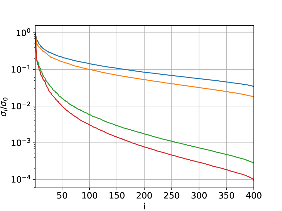
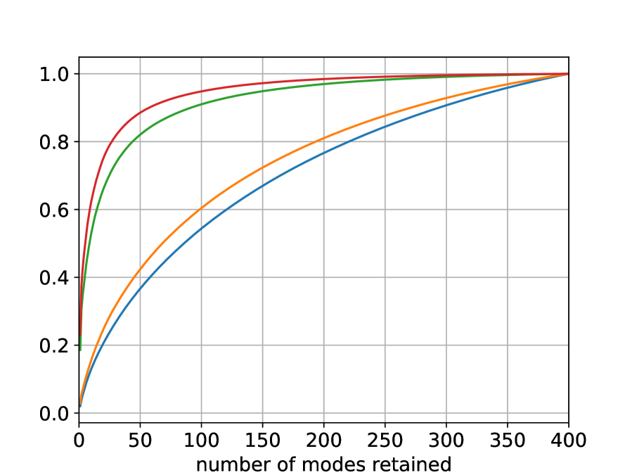
We applied the procedure described in Sec. 4.1 to generate to POD basis, starting from the 401 snapshots saved from the FOM simulation using the parameters specified in (44). The decay of the singular values of the potential vorticity fluctuations and stream function fluctuations in both layers is shown in Fig. 4 (a). We see that in both layers the decay for the potential vorticity fluctuation is much slower than the decay of the stream function fluctuation. The energy accumulation for all the fluctuations is shown in Fig. 4 (b). Typically, one would want to retain 99.99%percent99.9999.99\% of the singular value energy of the system. For this test case, it would mean that we need Nq1r=Nq2r=399superscriptsubscript𝑁subscript𝑞1𝑟superscriptsubscript𝑁subscript𝑞2𝑟399N_{q_{1}}^{r}=N_{q_{2}}^{r}=399, Nψ1r=398superscriptsubscript𝑁subscript𝜓1𝑟398N_{\psi_{1}}^{r}=398, Nψ2r=395superscriptsubscript𝑁subscript𝜓2𝑟395N_{\psi_{2}}^{r}=395. Obviously, these values are not viable since there would likely be no reduction in the computational time when compared to the FOM. If we were to retain only 50%percent5050\% of the energy, the number of basis functions would be reasonable for the stream function fluctuations (Nψ1r=8superscriptsubscript𝑁subscript𝜓1𝑟8N_{\psi_{1}}^{r}=8 and Nψ2r=5superscriptsubscript𝑁subscript𝜓2𝑟5N_{\psi_{2}}^{r}=5) but still too large for the potential vorticity fluctuations (Nq1r=86superscriptsubscript𝑁subscript𝑞1𝑟86N_{q_{1}}^{r}=86 and Nq2r=68superscriptsubscript𝑁subscript𝑞2𝑟68N_{q_{2}}^{r}=68).

Refer to caption
(a) Eigenvalue decay
Refer to caption
(b) Energy accumulation
Refer to caption
Figure 4: (a) Singular value decay and (b) energy accumulation of the potential vorticity fluctuations and stream function fluctuations in both layers.

Concerning the LSTM networks, for q1superscriptsubscript𝑞1q_{1}^{\prime} and q2superscriptsubscript𝑞2q_{2}^{\prime} we choose a single layer with 100100100 cells, while we use 333 hidden layers with 505050 cells each for ψ1superscriptsubscript𝜓1\psi_{1}^{\prime} and ψ2superscriptsubscript𝜓2\psi_{2}^{\prime}. This difference in the networks is due to the fact that, as we shall see, the time-averaged stream functions ψ~1subscript~𝜓1\widetilde{\psi}_{1} and ψ~2subscript~𝜓2\widetilde{\psi}_{2} have more complex patterns than the time-averaged vorticities q~1subscript~𝑞1\widetilde{q}_{1} and q~2subscript~𝑞2\widetilde{q}_{2}. The simpler structure of the patterns in q~1subscript~𝑞1\widetilde{q}_{1} and q~2subscript~𝑞2\widetilde{q}_{2} is such that using more than one layer would lead to overfitting. Concerning the optimization method, following [30] we choose a type of stochastic gradient descent widely used in machine learning [68] called Adam, which optimizes the weights by minimizing the mean square error (MSE). We summarize the hyperparameters for our LSTM networks in Table 1. We have intentionally left out of Table 1 the lookback window σLsubscript𝜎𝐿\sigma_{L} because we will show how the networks are sensitive to it.

Hyperparameters qlsubscriptsubscript𝑞𝑙\mathbf{\mathcal{M}}_{q_{l}} ψlsubscriptsubscript𝜓𝑙\mathbf{\mathcal{M}}_{\psi_{l}}
Number of layers 1 3
Number of cells per layer 100 50
Batch size 8 16
Epochs 500500500 500500500
Activation function tanh\tanh tanh\tanh
Validation 20%percent2020\% 20%percent2020\%
Testing : testing ratio 1:4:141:4 1:4:141:4
Loss function MSE MSE
Optimizer Adam Adam
Learning rate 1E-02 1E-02
Drop out probability - 0.1
Weight decay 1E-05 1E-05
Table 1: Hyperparameters for the LSTM network component of the POD-LSTM ROMs.

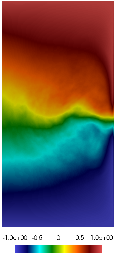
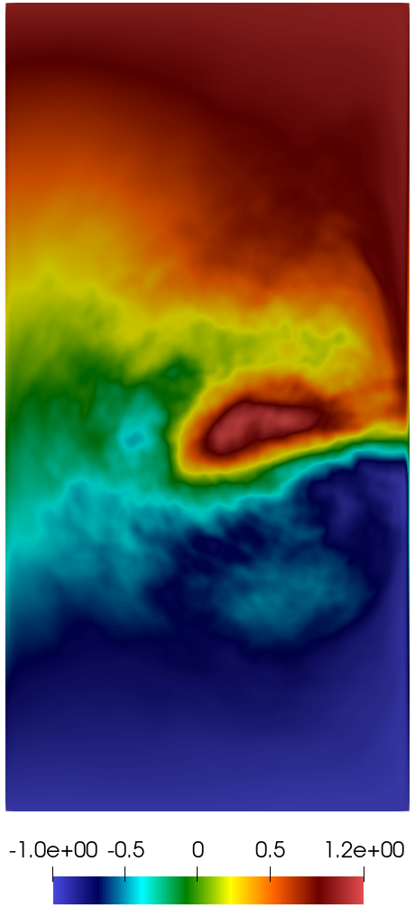
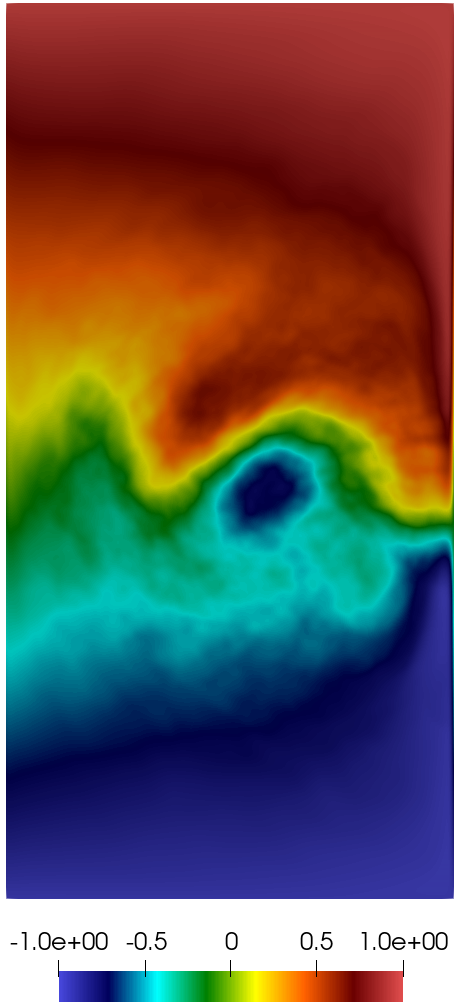
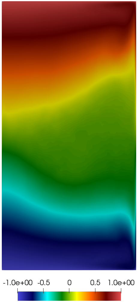
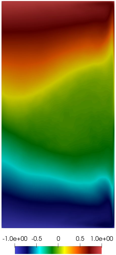
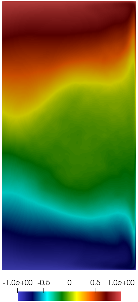
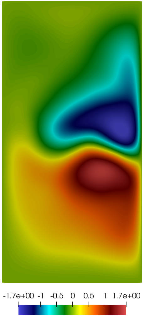
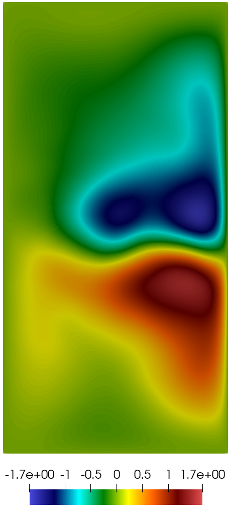
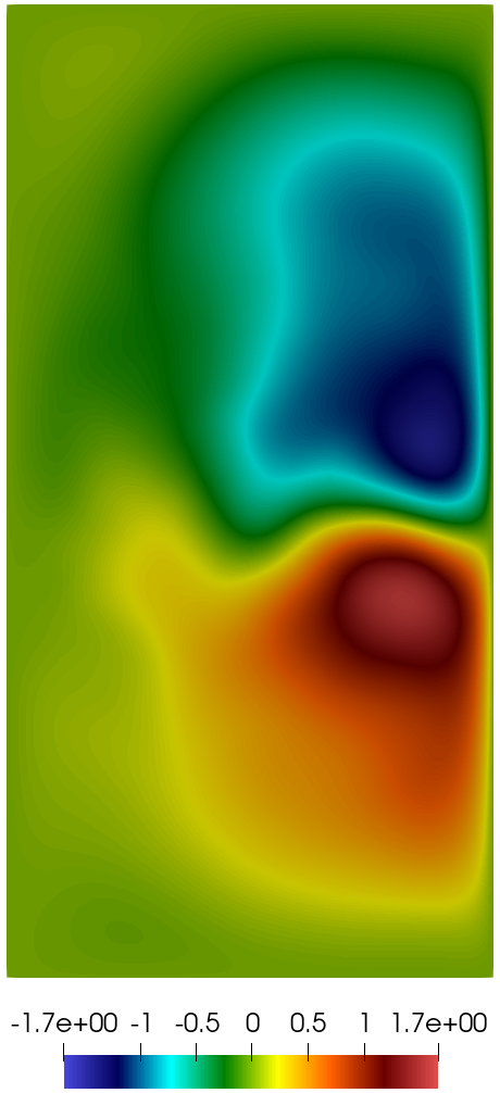
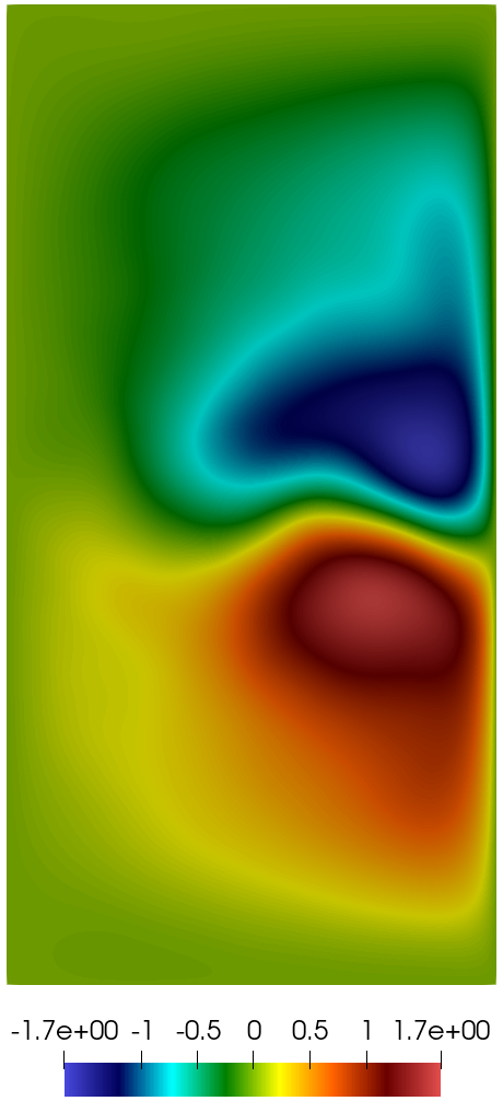
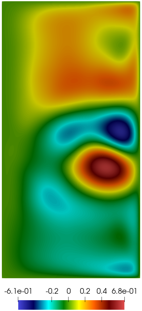
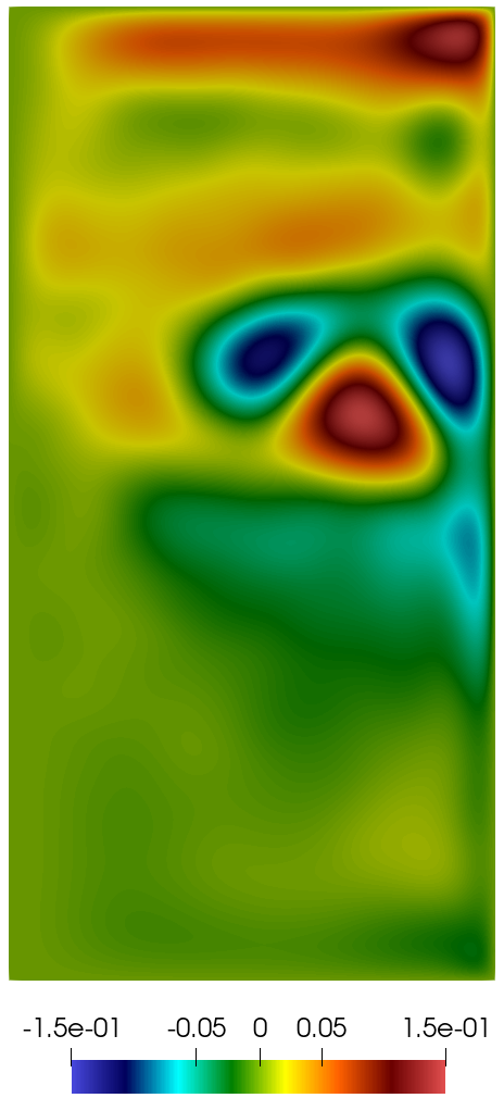
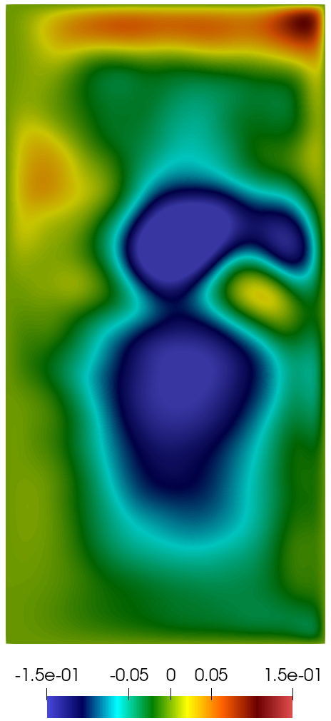
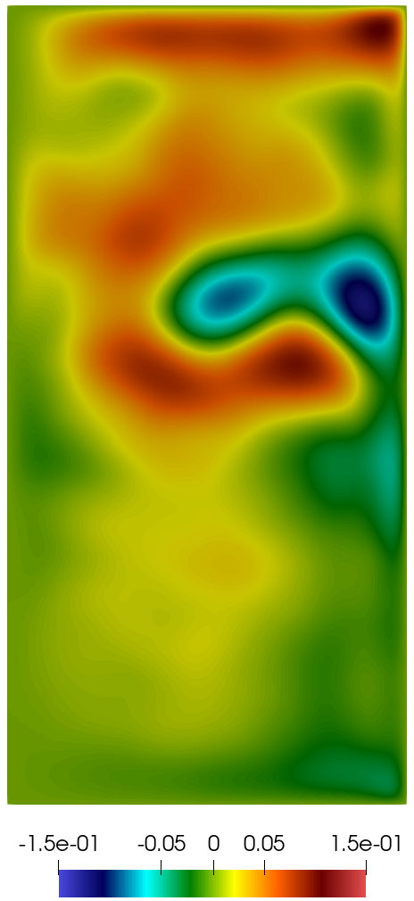
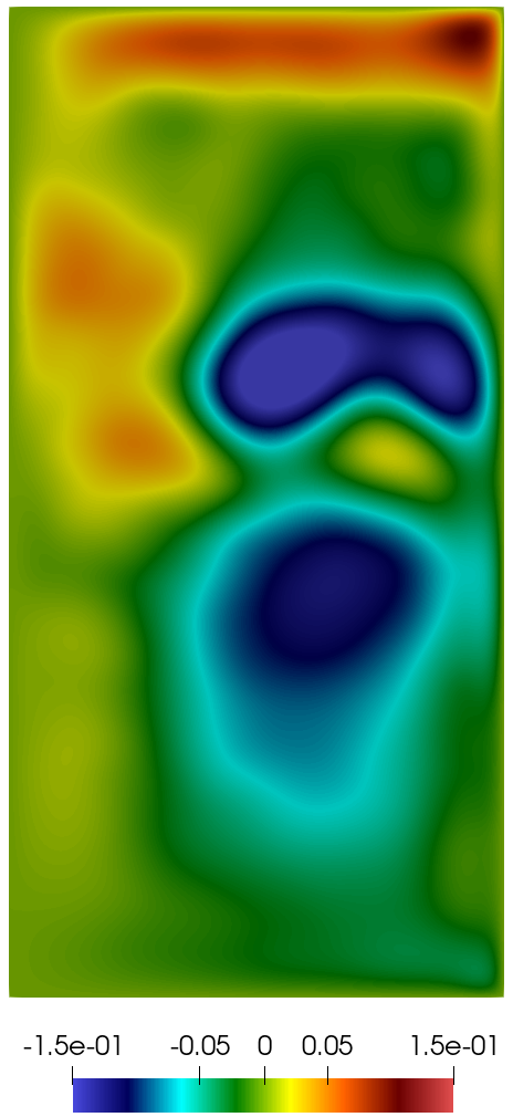
Let us start to assess the predictive performance of the POD-LSTM ROM for the vorticities. In order to prioritize computational time savings, we fix the number of modes to Nq1r=Nq2r=10superscriptsubscript𝑁subscript𝑞1𝑟superscriptsubscript𝑁subscript𝑞2𝑟10N_{q_{1}}^{r}=N_{q_{2}}^{r}=10, which translates to 14%percent1414\% of cumulative energy for q1superscriptsubscript𝑞1q_{1}^{\prime} and 17%percent1717\% for q2superscriptsubscript𝑞2q_{2}^{\prime}. Fig. 5 compares the time-averaged potential vorticity q~lsubscript~𝑞𝑙\widetilde{q}_{l}, l=1,2𝑙12l=1,2, computed over the predictive time interval [50,100]50100[50,100] by the FOM (first column) and the POD-LSTM ROM with different lookback windows (second to fifth columns). The ROM is able to capture the main features of the FOM solution for q~1subscript~𝑞1\widetilde{q}_{1} for all values of the lookback window. However, we see differences in how the ROM predicts the dark green region (small negative values) around the basin center (i.e., y=0𝑦0y=0), with value σL=1subscript𝜎𝐿1\sigma_{L}=1 providing the most accurate reconstruction of the FOM. In the case of q~2subscript~𝑞2\widetilde{q}_{2}, the POD-LSTM ROM struggles to reconstruct the FOM solution with σL=1,2,5subscript𝜎𝐿125\sigma_{L}=1,2,5 which give an incorrect oscillating behavior around the northern and southern regions of the ocean basin. The most accurate prediction of true q~2subscript~𝑞2\widetilde{q}_{2} is given by σL=10subscript𝜎𝐿10\sigma_{L}=10.

FOM σL=1subscript𝜎𝐿1\sigma_{L}=1 σL=2subscript𝜎𝐿2\sigma_{L}=2 σL=5subscript𝜎𝐿5\sigma_{L}=5 σL=10subscript𝜎𝐿10\sigma_{L}=10
q~1subscript~𝑞1\widetilde{q}_{1} Refer to caption Refer to caption Refer to caption Refer to caption Refer to caption
q~2subscript~𝑞2\widetilde{q}_{2} Refer to caption Refer to caption Refer to caption Refer to caption Refer to caption
Figure 5: q~1subscript~𝑞1\widetilde{q}_{1} and q~2subscript~𝑞2\widetilde{q}_{2} computed over the predictive time interval [50,100]50100[50,100] by the FOM (first column) and the POD-LSTM models q1subscriptsubscript𝑞1\mathbf{\mathcal{M}}_{q_{1}} (first row) and q2subscriptsubscript𝑞2\mathbf{\mathcal{M}}_{q_{2}} (second row) for different values of the lookback window σLsubscript𝜎𝐿\sigma_{L} (second to fifth columns).

To quantify the comparison in Fig. 5, Table 2 reports the errors εql(1)superscriptsubscript𝜀subscript𝑞𝑙1\varepsilon_{q_{l}}^{(1)} (45) and εql(2)superscriptsubscript𝜀subscript𝑞𝑙2\varepsilon_{q_{l}}^{(2)} (46), for l=1,2𝑙12l=1,2. Both metrics of accuracy confirm that σL=1subscript𝜎𝐿1\sigma_{L}=1 (resp., σL=10subscript𝜎𝐿10\sigma_{L}=10) provides the most accurate reconstruction of q~1subscript~𝑞1\widetilde{q}_{1} (resp., q~2subscript~𝑞2\widetilde{q}_{2}).

σLsubscript𝜎𝐿\sigma_{L} εq1(1)superscriptsubscript𝜀subscript𝑞11\varepsilon_{q_{1}}^{(1)} εq1(2)superscriptsubscript𝜀subscript𝑞12\varepsilon_{q_{1}}^{(2)} εq2(1)superscriptsubscript𝜀subscript𝑞21\varepsilon_{q_{2}}^{(1)} εq2(2)superscriptsubscript𝜀subscript𝑞22\varepsilon_{q_{2}}^{(2)}
1 2.716E-02 4.024E-02 8.880E-02 8.866E-02
2 7.837E-02 1.162E-01 6.902E-02 6.894E-02
5 4.953E-02 7.340E-02 8.639E-02 8.620E-02
10 7.465E-02 1.107E-01 4.424E-02 4.417E-02
Table 2: Error metrics εql(1)superscriptsubscript𝜀subscript𝑞𝑙1\varepsilon_{q_{l}}^{(1)} (45) and εql(2)superscriptsubscript𝜀subscript𝑞𝑙2\varepsilon_{q_{l}}^{(2)} (46), l=1,2𝑙12l=1,2, for different values of the lookback window σLsubscript𝜎𝐿\sigma_{L}.

So far, we have shown that q1subscriptsubscript𝑞1\mathbf{\mathcal{M}}_{q_{1}} with σL=1subscript𝜎𝐿1\sigma_{L}=1 and q2subscriptsubscript𝑞2\mathbf{\mathcal{M}}_{q_{2}} with σL=10subscript𝜎𝐿10\sigma_{L}=10 give rather accurate predictions of the time-averaged fields q~1subscript~𝑞1\widetilde{q}_{1} and q~2subscript~𝑞2\widetilde{q}_{2}, respectively. Next, we investigate how well they predict the dynamics of the system over the unseen time interval [50,100]50100[50,100]. Let us start with examining the first αl,1subscript𝛼𝑙1\alpha_{l,1} and third αl,3subscript𝛼𝑙3\alpha_{l,3} modal coefficients, l=1,2𝑙12l=1,2, computed using q1subscriptsubscript𝑞1\mathbf{\mathcal{M}}_{q_{1}} and q2subscriptsubscript𝑞2\mathbf{\mathcal{M}}_{q_{2}} with different lookback windows σLsubscript𝜎𝐿\sigma_{L}. We have chosen these coefficients, whose evolution in time is shown in in Fig. 67, because they are representative of all other modal coefficients. For q1subscript𝑞1q_{1}, we see that, although σL=1subscript𝜎𝐿1\sigma_{L}=1 does well in predicting the average, its time-dependent prediction is poor. This is in line with the findings in [30]. As σLsubscript𝜎𝐿\sigma_{L} increases, we see that both the reconstruction (t[10,50]𝑡1050t\in[10,50]) and the prediction (t(50,100]𝑡50100t\in(50,100]) of α1,1subscript𝛼11\alpha_{1,1} and α1,3subscript𝛼13\alpha_{1,3} improves, with σL=10subscript𝜎𝐿10\sigma_{L}=10 providing the most accurate results for both coefficients. Similar conclusions can be drawn for q2subscript𝑞2q_{2} from Fig. 7, i.e., the reconstructive and predictive ability of σL=1subscript𝜎𝐿1\sigma_{L}=1 is also poor and it tends to improve with the widening of the lookback window. Nonetheless, some differences can be noted between Fig. 6 and 7. The oscillations in α2,1subscript𝛼21\alpha_{2,1} and α2,3subscript𝛼23\alpha_{2,3} computed with σL=1subscript𝜎𝐿1\sigma_{L}=1 are more sustained than the oscillations in α1,1subscript𝛼11\alpha_{1,1} and α1,3subscript𝛼13\alpha_{1,3}, while the oscillations in α2,1subscript𝛼21\alpha_{2,1} and α2,3subscript𝛼23\alpha_{2,3} computed with σL=2subscript𝜎𝐿2\sigma_{L}=2 die down for t>80𝑡80t>80. Moreover, we see that the average of the oscillations in α2,3subscript𝛼23\alpha_{2,3} computed with σL=5subscript𝜎𝐿5\sigma_{L}=5 is off for t>70𝑡70t>70 with respect to the true average. We also note that σL=10subscript𝜎𝐿10\sigma_{L}=10 yields the best prediction of both q2subscript𝑞2q_{2} and its time-averaged quantity q~2subscript~𝑞2\widetilde{q}_{2}, while the values of σLsubscript𝜎𝐿\sigma_{L} are different for the first layer: σL=1subscript𝜎𝐿1\sigma_{L}=1 for q1subscript𝑞1q_{1} and σL=10subscript𝜎𝐿10\sigma_{L}=10 for q~1subscript~𝑞1\widetilde{q}_{1}.

Refer to caption
(a) α1,1(t),σL=1subscript𝛼11𝑡subscript𝜎𝐿1\alpha_{1,1}(t),\sigma_{L}=1
Refer to caption
(b) α1,3(t),σL=1subscript𝛼13𝑡subscript𝜎𝐿1\alpha_{1,3}(t),\sigma_{L}=1
Refer to caption
(c) α1,1(t),σL=2subscript𝛼11𝑡subscript𝜎𝐿2\alpha_{1,1}(t),\sigma_{L}=2
Refer to caption
(d) α1,3(t),σL=2subscript𝛼13𝑡subscript𝜎𝐿2\alpha_{1,3}(t),\sigma_{L}=2
Refer to caption
(e) α1,1(t),σL=5subscript𝛼11𝑡subscript𝜎𝐿5\alpha_{1,1}(t),\sigma_{L}=5
Refer to caption
(f) α1,3(t),σL=5subscript𝛼13𝑡subscript𝜎𝐿5\alpha_{1,3}(t),\sigma_{L}=5
Refer to caption
(g) α1,1(t),σL=10subscript𝛼11𝑡subscript𝜎𝐿10\alpha_{1,1}(t),\sigma_{L}=10
Refer to caption
(h) α1,3(t),σL=10subscript𝛼13𝑡subscript𝜎𝐿10\alpha_{1,3}(t),\sigma_{L}=10
Refer to caption
Figure 6: Time evolution of the first α1,1subscript𝛼11\alpha_{1,1} (left) and third α1,3subscript𝛼13\alpha_{1,3} (right) modal coefficients for q1subscript𝑞1q_{1} over the time interval [10,100]10100[10,100] for different values of the lookback window σLsubscript𝜎𝐿\sigma_{L}.
Refer to caption
(a) α2,1(t),σL=1subscript𝛼21𝑡subscript𝜎𝐿1\alpha_{2,1}(t),\sigma_{L}=1
Refer to caption
(b) α2,3(t),σL=1subscript𝛼23𝑡subscript𝜎𝐿1\alpha_{2,3}(t),\sigma_{L}=1
Refer to caption
(c) α2,1(t),σL=2subscript𝛼21𝑡subscript𝜎𝐿2\alpha_{2,1}(t),\sigma_{L}=2
Refer to caption
(d) α2,3(t),σL=2subscript𝛼23𝑡subscript𝜎𝐿2\alpha_{2,3}(t),\sigma_{L}=2
Refer to caption
(e) α2,1(t),σL=5subscript𝛼21𝑡subscript𝜎𝐿5\alpha_{2,1}(t),\sigma_{L}=5
Refer to caption
(f) α2,3(t),σL=5subscript𝛼23𝑡subscript𝜎𝐿5\alpha_{2,3}(t),\sigma_{L}=5
Refer to caption
(g) α2,1(t),σL=10subscript𝛼21𝑡subscript𝜎𝐿10\alpha_{2,1}(t),\sigma_{L}=10
Refer to caption
(h) α2,3(t),σL=10subscript𝛼23𝑡subscript𝜎𝐿10\alpha_{2,3}(t),\sigma_{L}=10
Refer to caption
Figure 7: Time evolution of the first α2,1subscript𝛼21\alpha_{2,1} (left) and third α2,3subscript𝛼23\alpha_{2,3} (right) modal coefficients for q2subscript𝑞2q_{2} over the time interval [10,100]10100[10,100] for different values of the lookback window σLsubscript𝜎𝐿\sigma_{L}.

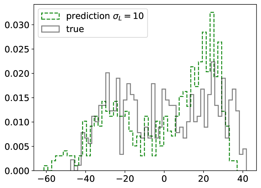
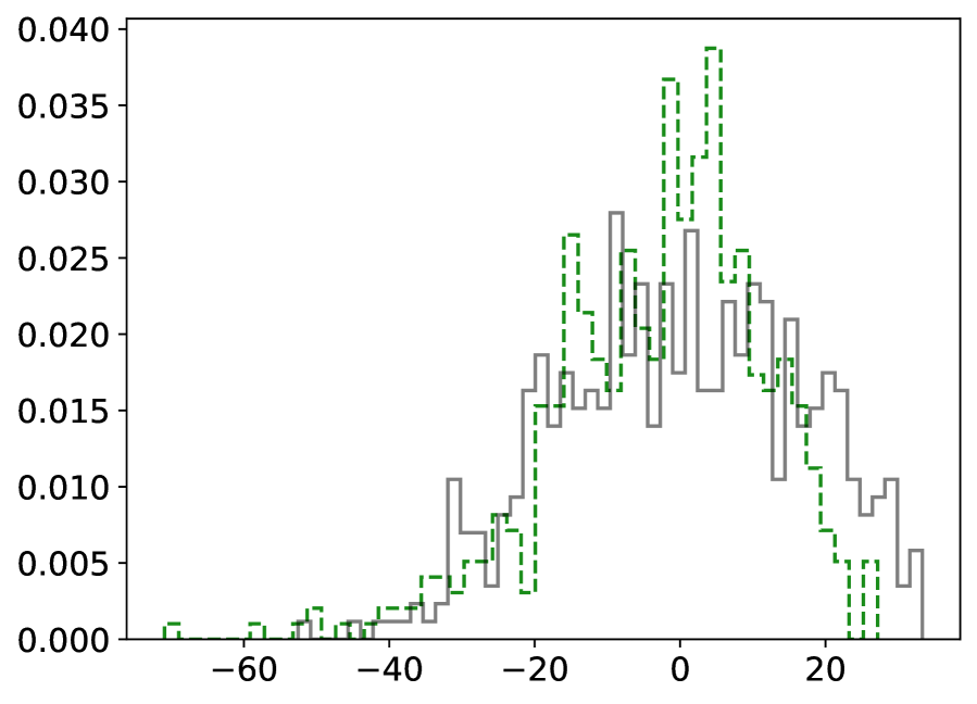
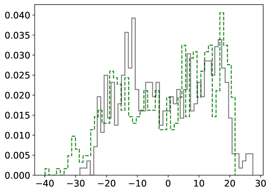
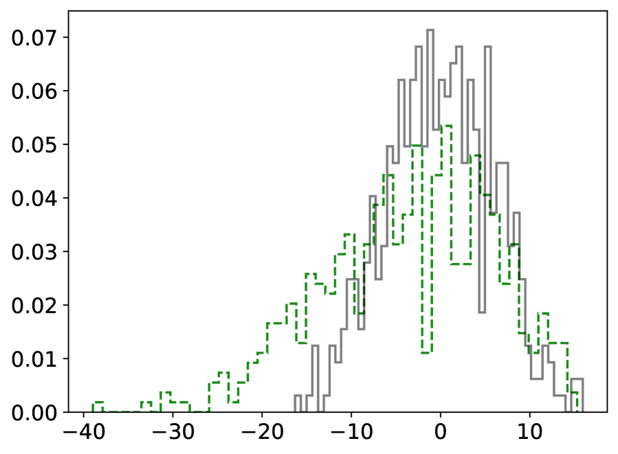
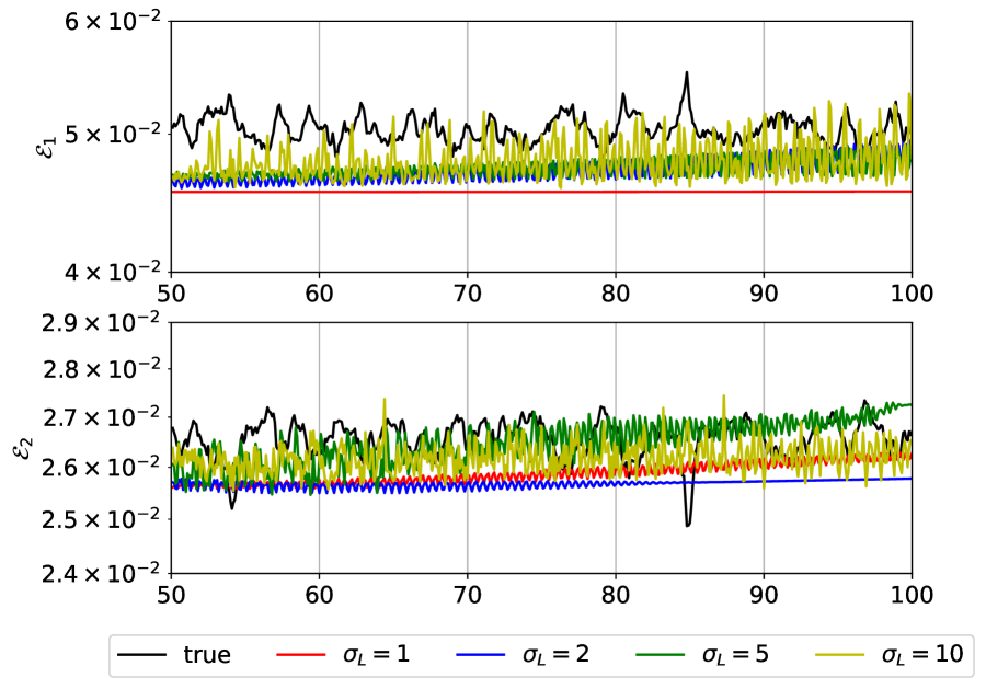
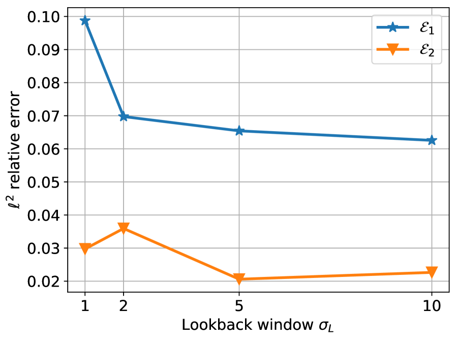
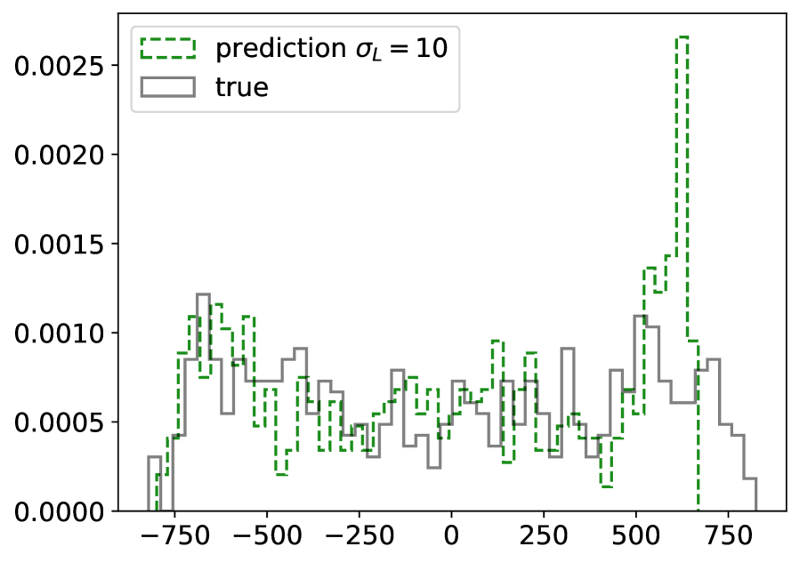
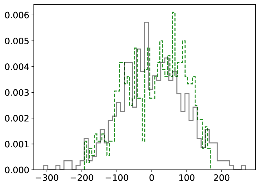
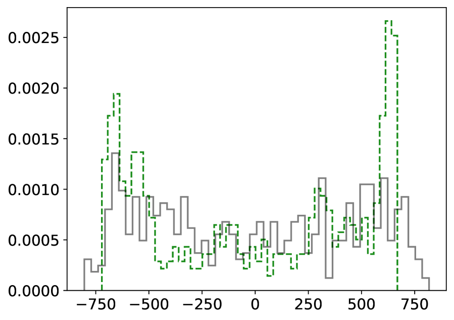
Fig. 8 compares the probability mass functions (PMF), i.e., a function that gives the probability of each possible value for a discrete random variable, of the first and third modal coefficients over the unseen time interval [50,100]50100[50,100] for the FOM solution projected onto the appropriate reduced space with the counterparts computed by q1subscriptsubscript𝑞1\mathbf{\mathcal{M}}_{q_{1}} and q2subscriptsubscript𝑞2\mathbf{\mathcal{M}}_{q_{2}} for σL=10subscript𝜎𝐿10\sigma_{L}=10. We observe a good agreement. The comparison in terms of enstrophy evolution (47) is shown in Fig. 9 (left) for different values of σLsubscript𝜎𝐿\sigma_{L}. For the top layer, σL=1subscript𝜎𝐿1\sigma_{L}=1 gives the worst prediction, which is consistent with our observation from Fig. 6, while the best prediction (i.e., lowest relative L2superscript𝐿2L^{2} error) is for σL=10subscript𝜎𝐿10\sigma_{L}=10. For σL=10subscript𝜎𝐿10\sigma_{L}=10, we obtain a good prediction also for the enstrophy in the bottom layer, although not the best in the relative L2superscript𝐿2L^{2} norm. See Fig. 9 (right).

Refer to caption
(a) α1,1(t)subscript𝛼11𝑡\alpha_{1,1}(t)
Refer to caption
(b) α1,3(t)subscript𝛼13𝑡\alpha_{1,3}(t)
Refer to caption
(c) α2,1(t)subscript𝛼21𝑡\alpha_{2,1}(t)
Refer to caption
(d) α2,3(t)subscript𝛼23𝑡\alpha_{2,3}(t)
Figure 8: Probability mass functions of the first and third modal coefficients of q1subscript𝑞1q_{1} (top row) and q2subscript𝑞2q_{2} (bottom row) over time interval [50,100]50100[50,100]: comparison between true value, i.e., for the FOM solution projected onto the appropriate reduced space, and the value computed by q1subscriptsubscript𝑞1\mathbf{\mathcal{M}}_{q_{1}} and q2subscriptsubscript𝑞2\mathbf{\mathcal{M}}_{q_{2}} for σL=10subscript𝜎𝐿10\sigma_{L}=10.
Refer to caption
Refer to caption
Figure 9: Time evolution of the enstrophy for the top layer 1subscript1\mathcal{E}_{1} (top left) and the bottom layer 2subscript2\mathcal{E}_{2} (bottom left) computed using the FOM and the POD-LSTM ROM with different lookback window σLsubscript𝜎𝐿\sigma_{L}. The corresponding relative L2superscript𝐿2L^{2} error is shown on the right.

In light of the results presented so far, we fix the lookback window to σL=10subscript𝜎𝐿10\sigma_{L}=10 for both q1subscriptsubscript𝑞1\mathbf{\mathcal{M}}_{q_{1}} and q2subscriptsubscript𝑞2\mathbf{\mathcal{M}}_{q_{2}}. Next, we vary the number of modes retained. Fig. 10 shows the time-averaged potential vorticities q~1subscript~𝑞1\widetilde{q}_{1} and q~2subscript~𝑞2\widetilde{q}_{2} computed using the FOM and the POD-LSTM ROM with different numbers of modal basis functions retained. We see that q~1subscript~𝑞1\widetilde{q}_{1} given by the ROM with Nq1r=4,8superscriptsubscript𝑁subscript𝑞1𝑟48N_{q_{1}}^{r}=4,8 cannot correctly capture the solution around the center of the basin. The ROM with Nq1r=10superscriptsubscript𝑁subscript𝑞1𝑟10N_{q_{1}}^{r}=10 improves the solution, however the most accurate ROM solution is obtained with Nq1r=2superscriptsubscript𝑁subscript𝑞1𝑟2N_{q_{1}}^{r}=2. It could be argued that also for q~2subscript~𝑞2\widetilde{q}_{2} the most accurate ROM solution is obtained with Nq2r=2superscriptsubscript𝑁subscript𝑞2𝑟2N_{q_{2}}^{r}=2. This is rather remarkable since with Nq1r=2superscriptsubscript𝑁subscript𝑞1𝑟2N_{q_{1}}^{r}=2 (resp., Nq2r=2superscriptsubscript𝑁subscript𝑞2𝑟2N_{q_{2}}^{r}=2) we retain only 5% (resp., 6%) of the cumulative eigenvalue energy (31). To complement the qualitative assessment in Fig. 10, Table 3 reports the errors εql(1)superscriptsubscript𝜀subscript𝑞𝑙1\varepsilon_{q_{l}}^{(1)} (45) and εql(2)superscriptsubscript𝜀subscript𝑞𝑙2\varepsilon_{q_{l}}^{(2)} (46), for l=1,2𝑙12l=1,2, and the relative L2superscript𝐿2L^{2} error of the enstrophy in both layers.

FOM Nqlr=2superscriptsubscript𝑁subscript𝑞𝑙𝑟2N_{q_{l}}^{r}=2 Nqlr=4superscriptsubscript𝑁subscript𝑞𝑙𝑟4N_{q_{l}}^{r}=4 Nqlr=8superscriptsubscript𝑁subscript𝑞𝑙𝑟8N_{q_{l}}^{r}=8 Nqlr=10superscriptsubscript𝑁subscript𝑞𝑙𝑟10N_{q_{l}}^{r}=10
q~1subscript~𝑞1\widetilde{q}_{1} Refer to caption Refer to caption Refer to caption Refer to caption Refer to caption
q~2subscript~𝑞2\widetilde{q}_{2} Refer to caption Refer to caption Refer to caption Refer to caption Refer to caption
Figure 10: Time-averaged vorticities q~1subscript~𝑞1\widetilde{q}_{1} (top) and q~2subscript~𝑞2\widetilde{q}_{2} (bottom) over the predictive time interval [50,100]50100[50,100] computed by FOM (first column) and POD-LSTM ROM with Nqlr=2,4,8,10superscriptsubscript𝑁subscript𝑞𝑙𝑟24810N_{q_{l}}^{r}=2,4,8,10 (second to fifth columns).

Next, we look at the evolution in time of second αl,2subscript𝛼𝑙2\alpha_{l,2} modal coefficient computed using qlsubscriptsubscript𝑞𝑙\mathbf{\mathcal{M}}_{q_{l}} with different Nqlrsuperscriptsubscript𝑁subscript𝑞𝑙𝑟N_{q_{l}}^{r}, l=1,2𝑙12l=1,2. This evolution, shown in Fig. 11, is chosen to be representative of the evolutions of all other modal coefficients. We see that, even though Nq1r=2superscriptsubscript𝑁subscript𝑞1𝑟2N_{q_{1}}^{r}=2 gives lower errors in the metrics in Table 3, both the reconstruction and prediction of α1,2subscript𝛼12\alpha_{1,2} are inferior to those obtained with Nq1r=10superscriptsubscript𝑁subscript𝑞1𝑟10N_{q_{1}}^{r}=10. Compare Fig. 11 (a) and (d). This, combined with the fact that the L2superscript𝐿2L^{2} relative error of 1subscript1\mathcal{E}_{1} for Nq1r=10superscriptsubscript𝑁subscript𝑞1𝑟10N_{q_{1}}^{r}=10 is about 1.5 times smaller than the error Nq1r=2superscriptsubscript𝑁subscript𝑞1𝑟2N_{q_{1}}^{r}=2 (see Table 3), leads us to believe that q1subscriptsubscript𝑞1\mathbf{\mathcal{M}}_{q_{1}} with Nq1r=10superscriptsubscript𝑁subscript𝑞1𝑟10N_{q_{1}}^{r}=10 can predict time-dependent quantities with more accuracy than q1subscriptsubscript𝑞1\mathbf{\mathcal{M}}_{q_{1}} with Nq1r=2superscriptsubscript𝑁subscript𝑞1𝑟2N_{q_{1}}^{r}=2. Further, Table 3 and Fig. 11 (e)-(h) indicate that q2subscriptsubscript𝑞2\mathbf{\mathcal{M}}_{q_{2}} with Nq2r=10superscriptsubscript𝑁subscript𝑞2𝑟10N_{q_{2}}^{r}=10 results in the most accurate prediction of the time-averaged field q~2subscript~𝑞2\widetilde{q}_{2}, time evolution reconstruction of 2subscript2\mathcal{E}_{2}, and the second modal coefficient α2,2subscript𝛼22\alpha_{2,2}.

Nq1rsuperscriptsubscript𝑁subscript𝑞1𝑟N_{q_{1}}^{r} δq1subscript𝛿subscript𝑞1\delta_{q_{1}} εq1(1)superscriptsubscript𝜀subscript𝑞11\varepsilon_{q_{1}}^{(1)} εq1(2)superscriptsubscript𝜀subscript𝑞12\varepsilon_{q_{1}}^{(2)} 1subscript1\mathcal{E}_{1} rel. err.
2 0.05 3.999E-02 5.922E-02 9.288E-02
4 0.07 1.824E-01 2.705E-01 4.528E-02
8 0.12 9.429E-02 1.398E-01 5.705E-02
10 0.13 7.465E-02 1.107E-01 6.256E-02
Nq2rsuperscriptsubscript𝑁subscript𝑞2𝑟N_{q_{2}}^{r} δq2subscript𝛿subscript𝑞2\delta_{q_{2}} εq2(1)superscriptsubscript𝜀subscript𝑞21\varepsilon_{q_{2}}^{(1)} εq2(2)superscriptsubscript𝜀subscript𝑞22\varepsilon_{q_{2}}^{(2)} 2subscript2\mathcal{E}_{2} rel. err.
2 0.06 2.428E-02 4.798E-02 3.880E-02
4 0.09 2.727E-02 5.385E-02 3.006E-02
8 0.14 2.605E-02 5.146E-02 2.831E-01
10 0.16 2.235E-02 4.417E-02 2.266E-02
Table 3: Fraction of retained eigenvalue energy δqlsubscript𝛿subscript𝑞𝑙\delta_{q_{l}}, error metrics εql(1)superscriptsubscript𝜀subscript𝑞𝑙1\varepsilon_{q_{l}}^{(1)} (45) and εql(2)superscriptsubscript𝜀subscript𝑞𝑙2\varepsilon_{q_{l}}^{(2)} (46), and relative L2superscript𝐿2L^{2} error for enstrophy lsubscript𝑙\mathcal{E}_{l} (47), l=1,2𝑙12l=1,2, for different numbers of POD modes retained.
Refer to caption
(a) α1,2(t),Nq1r=2subscript𝛼12𝑡superscriptsubscript𝑁subscript𝑞1𝑟2\alpha_{1,2}(t),N_{q_{1}}^{r}=2
Refer to caption
(b) α1,2(t),Nq1r=4subscript𝛼12𝑡superscriptsubscript𝑁subscript𝑞1𝑟4\alpha_{1,2}(t),N_{q_{1}}^{r}=4
Refer to caption
(c) α1,2(t),Nq1r=8subscript𝛼12𝑡superscriptsubscript𝑁subscript𝑞1𝑟8\alpha_{1,2}(t),N_{q_{1}}^{r}=8
Refer to caption
(d) α1,2(t),Nq1r=10subscript𝛼12𝑡superscriptsubscript𝑁subscript𝑞1𝑟10\alpha_{1,2}(t),N_{q_{1}}^{r}=10
Refer to caption
(e) α2,2(t),Nq2r=2subscript𝛼22𝑡superscriptsubscript𝑁subscript𝑞2𝑟2\alpha_{2,2}(t),N_{q_{2}}^{r}=2
Refer to caption
(f) α2,2(t),Nq2r=4subscript𝛼22𝑡superscriptsubscript𝑁subscript𝑞2𝑟4\alpha_{2,2}(t),N_{q_{2}}^{r}=4
Refer to caption
(g) α2,2(t),Nq2r=8subscript𝛼22𝑡superscriptsubscript𝑁subscript𝑞2𝑟8\alpha_{2,2}(t),N_{q_{2}}^{r}=8
Refer to caption
(h) α2,2(t),Nq2r=10subscript𝛼22𝑡superscriptsubscript𝑁subscript𝑞2𝑟10\alpha_{2,2}(t),N_{q_{2}}^{r}=10
Refer to caption
Figure 11: Time evolution of the second modal coefficient αl,2subscript𝛼𝑙2\alpha_{l,2} over the time interval [10,100]10100[10,100] for different numbers of retained POD basis function Nqlrsuperscriptsubscript𝑁subscript𝑞𝑙𝑟N_{q_{l}}^{r}, l=1,2𝑙12l=1,2.

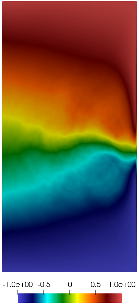
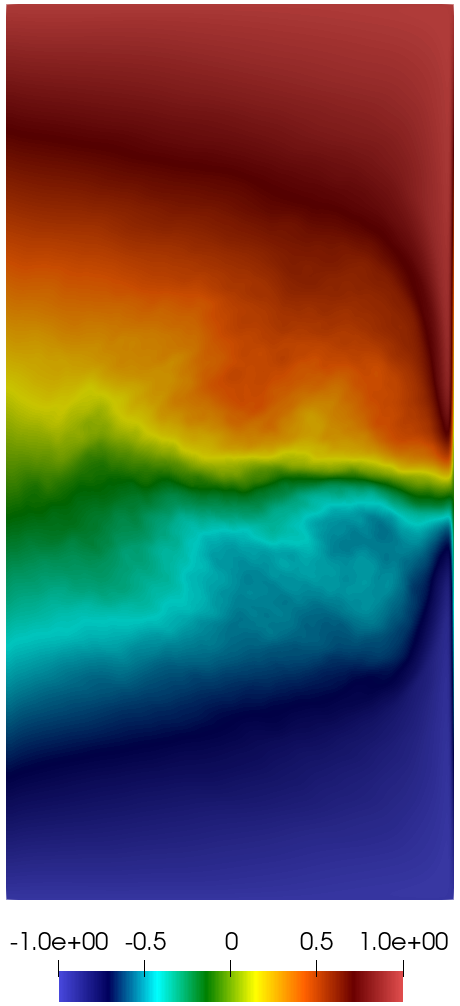
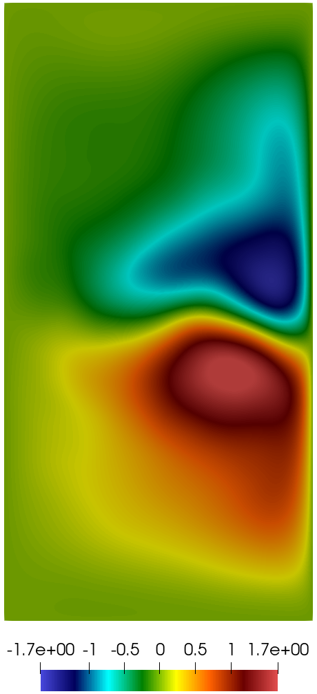
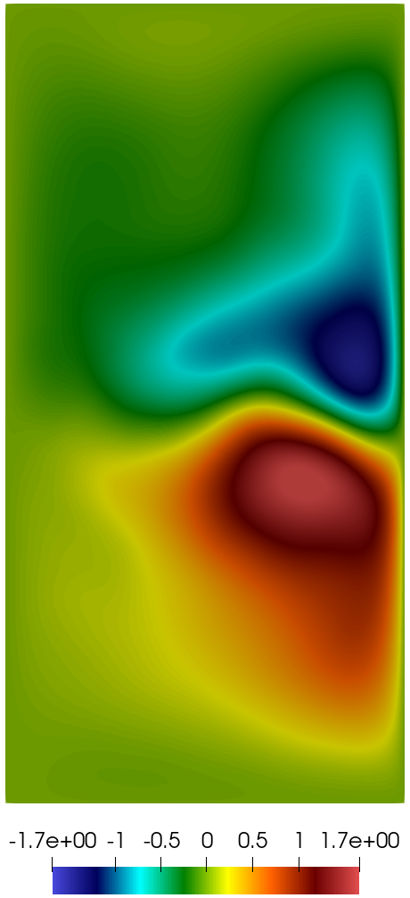
Let us shift our focus to the predictive performance of the POD-LSTM ROM for the stream functions ψ1subscript𝜓1\psi_{1} and ψ2subscript𝜓2\psi_{2}. We recall that the hyperparameters of the LSTM network are reported in Table 1, third column. Following the analysis for q1subscriptsubscript𝑞1\mathbf{\mathcal{M}}_{q_{1}} and q2subscriptsubscript𝑞2\mathbf{\mathcal{M}}_{q_{2}}, we first fix the number of retained POD basis functions to Nψ1r=Nψ2r=10superscriptsubscript𝑁subscript𝜓1𝑟superscriptsubscript𝑁subscript𝜓2𝑟10N_{\psi_{1}}^{r}=N_{\psi_{2}}^{r}=10, which means retaining 54%percent5454\% and 64%percent6464\% of the cumulative singular value energy for ψ1superscriptsubscript𝜓1\psi_{1}^{\prime} and ψ2superscriptsubscript𝜓2\psi_{2}^{\prime}, respectively. Fig. 12 compares the true ψ~1subscript~𝜓1\widetilde{\psi}_{1} and ψ~2subscript~𝜓2\widetilde{\psi}_{2} (first column) with ψ~1subscript~𝜓1\widetilde{\psi}_{1} and ψ~2subscript~𝜓2\widetilde{\psi}_{2} computed by the POD-LSTM ROM with different values of σLsubscript𝜎𝐿\sigma_{L} (second to fifth columns). While the POD-LSTM ROM manages to capture the correct number of gyres in ψ~1subscript~𝜓1\widetilde{\psi}_{1} for all values of σLsubscript𝜎𝐿\sigma_{L} and gets a good approximation of the gyres shape for σL=1,10subscript𝜎𝐿110\sigma_{L}=1,10, it cannot reliably predict ψ~2subscript~𝜓2\widetilde{\psi}_{2} for lower values of σLsubscript𝜎𝐿\sigma_{L}. However, for σL=10subscript𝜎𝐿10\sigma_{L}=10 the POD-LSTM ROM produces the correct shape of the gyres in ψ~2subscript~𝜓2\widetilde{\psi}_{2}, especially the outer gyres that can be harder to predict [39].

FOM σL=1subscript𝜎𝐿1\sigma_{L}=1 σL=2subscript𝜎𝐿2\sigma_{L}=2 σL=5subscript𝜎𝐿5\sigma_{L}=5 σL=10subscript𝜎𝐿10\sigma_{L}=10
ψ~1subscript~𝜓1\widetilde{\psi}_{1} Refer to caption Refer to caption Refer to caption Refer to caption Refer to caption
ψ~2subscript~𝜓2\widetilde{\psi}_{2} Refer to caption Refer to caption Refer to caption Refer to caption Refer to caption
Figure 12: ψ~1subscript~𝜓1\widetilde{\psi}_{1} and ψ~2subscript~𝜓2\widetilde{\psi}_{2} computed over the predictive time interval [50,100]50100[50,100] by the FOM (first column) and the POD-LSTM ψ1subscriptsubscript𝜓1\mathbf{\mathcal{M}}_{\psi_{1}} (first row) and ψ2subscriptsubscript𝜓2\mathbf{\mathcal{M}}_{\psi_{2}} (second row) for different values of the lookback window σLsubscript𝜎𝐿\sigma_{L} (second to fifth columns).

To quantify the comparison in Fig. 12, Table 4 reports the errors εψl(1)superscriptsubscript𝜀subscript𝜓𝑙1\varepsilon_{\psi_{l}}^{(1)} (45) and εψl(2)superscriptsubscript𝜀subscript𝜓𝑙2\varepsilon_{\psi_{l}}^{(2)} (46) for l=1,2𝑙12l=1,2. In both metrics, σL=10subscript𝜎𝐿10\sigma_{L}=10 produces the lowest errors.

σLsubscript𝜎𝐿\sigma_{L} εψ1(1)superscriptsubscript𝜀subscript𝜓11\varepsilon_{\psi_{1}}^{(1)} εψ1(2)superscriptsubscript𝜀subscript𝜓12\varepsilon_{\psi_{1}}^{(2)} εψ2(1)superscriptsubscript𝜀subscript𝜓21\varepsilon_{\psi_{2}}^{(1)} εψ2(2)superscriptsubscript𝜀subscript𝜓22\varepsilon_{\psi_{2}}^{(2)}
1 1.102E-01 1.911E-01 1.206E-01 6.579E-01
2 1.671E-01 2.900E-01 1.630E-01 8.893E-01
5 1.654E-01 2.870E-01 9.909E-02 5.406E-01
10 6.041E-02 1.048E-01 4.543E-02 2.479E-01
Table 4: Error metrics εψl(1)superscriptsubscript𝜀subscript𝜓𝑙1\varepsilon_{\psi_{l}}^{(1)} (45) and εψl(2)superscriptsubscript𝜀subscript𝜓𝑙2\varepsilon_{\psi_{l}}^{(2)} (46), l=1,2𝑙12l=1,2, for different values of the lookback window σLsubscript𝜎𝐿\sigma_{L}.

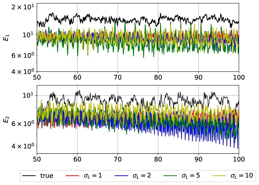
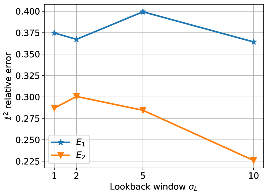
In order to understand the time-dependent predictive performance of POD-LSTM ROM, we show the first βl,1subscript𝛽𝑙1\beta_{l,1} and third βl,3subscript𝛽𝑙3\beta_{l,3} modal coefficients computed using ψlsubscriptsubscript𝜓𝑙\mathbf{\mathcal{M}}_{\psi_{l}}, l=1,2𝑙12l=1,2, with different σLsubscript𝜎𝐿\sigma_{L} in Fig. 13-14. While β1,1subscript𝛽11\beta_{1,1} and β2,1subscript𝛽21\beta_{2,1} are rather well approximated regardless of the value of σLsubscript𝜎𝐿\sigma_{L}, for β1,3subscript𝛽13\beta_{1,3} and β2,3subscript𝛽23\beta_{2,3} we see that σL=10subscript𝜎𝐿10\sigma_{L}=10 gives the most accurate reconstructions and predictions. Fig. 15 compares the probability mass functions of the first and third modal coefficients over the unseen time interval [50,100]50100[50,100] for the FOM solution projected onto the appropriate reduced space with the counterparts computed by ψ1subscriptsubscript𝜓1\mathbf{\mathcal{M}}_{\psi_{1}} and ψ2subscriptsubscript𝜓2\mathbf{\mathcal{M}}_{\psi_{2}} for σL=10subscript𝜎𝐿10\sigma_{L}=10. The true and predicted PMFs are in good agreement, except for β2,3subscript𝛽23\beta_{2,3}. The comparison in terms of kinetic energy evolution (48) is shown in Fig. 16 (left) for different values of σLsubscript𝜎𝐿\sigma_{L}. We see that the POD-LSTM ROM underestimates the kinetic energy for either layer, which we suspect is caused by the retention of only roughly half of the cumulative singular value energy. The lowest relative L2superscript𝐿2L^{2} errors with respect to the true kinetic energy of the system is given by σL=10subscript𝜎𝐿10\sigma_{L}=10. See the right panel of Fig. 16 right.

Refer to caption
(a) β1,1(t),σL=1subscript𝛽11𝑡subscript𝜎𝐿1\beta_{1,1}(t),\sigma_{L}=1
Refer to caption
(b) β1,3(t),σL=1subscript𝛽13𝑡subscript𝜎𝐿1\beta_{1,3}(t),\sigma_{L}=1
Refer to caption
(c) β1,1(t),σL=2subscript𝛽11𝑡subscript𝜎𝐿2\beta_{1,1}(t),\sigma_{L}=2
Refer to caption
(d) β1,3(t),σL=2subscript𝛽13𝑡subscript𝜎𝐿2\beta_{1,3}(t),\sigma_{L}=2
Refer to caption
(e) β1,1(t),σL=5subscript𝛽11𝑡subscript𝜎𝐿5\beta_{1,1}(t),\sigma_{L}=5
Refer to caption
(f) β1,3(t),σL=5subscript𝛽13𝑡subscript𝜎𝐿5\beta_{1,3}(t),\sigma_{L}=5
Refer to caption
(g) β1,1(t),σL=10subscript𝛽11𝑡subscript𝜎𝐿10\beta_{1,1}(t),\sigma_{L}=10
Refer to caption
(h) β1,3(t),σL=10subscript𝛽13𝑡subscript𝜎𝐿10\beta_{1,3}(t),\sigma_{L}=10
Refer to caption
Figure 13: Time evolution of the first β1,1subscript𝛽11\beta_{1,1} (left) and third β1,3subscript𝛽13\beta_{1,3} (right) modal coefficients for ψ1subscript𝜓1\psi_{1} over the time interval [10,100]10100[10,100] for different values of the lookback window σLsubscript𝜎𝐿\sigma_{L}.
Refer to caption
(a) β2,1(t),σL=1subscript𝛽21𝑡subscript𝜎𝐿1\beta_{2,1}(t),\sigma_{L}=1
Refer to caption
(b) β2,3(t),σL=1subscript𝛽23𝑡subscript𝜎𝐿1\beta_{2,3}(t),\sigma_{L}=1
Refer to caption
(c) β2,1(t),σL=2subscript𝛽21𝑡subscript𝜎𝐿2\beta_{2,1}(t),\sigma_{L}=2
Refer to caption
(d) β2,3(t),σL=2subscript𝛽23𝑡subscript𝜎𝐿2\beta_{2,3}(t),\sigma_{L}=2
Refer to caption
(e) β2,1(t),σL=5subscript𝛽21𝑡subscript𝜎𝐿5\beta_{2,1}(t),\sigma_{L}=5
Refer to caption
(f) β2,3(t),σL=5subscript𝛽23𝑡subscript𝜎𝐿5\beta_{2,3}(t),\sigma_{L}=5
Refer to caption
(g) β2,1(t),σL=10subscript𝛽21𝑡subscript𝜎𝐿10\beta_{2,1}(t),\sigma_{L}=10
Refer to caption
(h) β2,3(t),σL=10subscript𝛽23𝑡subscript𝜎𝐿10\beta_{2,3}(t),\sigma_{L}=10
Refer to caption
Figure 14: Time evolution of the first β2,1subscript𝛽21\beta_{2,1} (left) and third β2,3subscript𝛽23\beta_{2,3} (right) modal coefficients for ψ2subscript𝜓2\psi_{2} over the time interval [10,100]10100[10,100] for different values of the lookback window σLsubscript𝜎𝐿\sigma_{L}.
Refer to caption
(a) β1,1(t)subscript𝛽11𝑡\beta_{1,1}(t)
Refer to caption
(b) β1,3(t)subscript𝛽13𝑡\beta_{1,3}(t)
Refer to caption
(c) β2,1(t)subscript𝛽21𝑡\beta_{2,1}(t)
Refer to caption
(d) β2,3(t)subscript𝛽23𝑡\beta_{2,3}(t)
Figure 15: Probability mass functions of the first and third modal coefficients of ψ1subscript𝜓1\psi_{1} (top row) and ψ2subscript𝜓2\psi_{2} (bottom row) over time interval [50,100]50100[50,100]: comparison between true value, i.e., for the FOM solution projected onto the appropriate reduced space, and the value computed by ψ1subscriptsubscript𝜓1\mathbf{\mathcal{M}}_{\psi_{1}} and ψ2subscriptsubscript𝜓2\mathbf{\mathcal{M}}_{\psi_{2}} for σL=10subscript𝜎𝐿10\sigma_{L}=10.
Refer to caption
Refer to caption
Figure 16: Time evolution of the kinetic energy for the top layer 1subscript1\mathcal{E}_{1} (top left) and the bottom layer 2subscript2\mathcal{E}_{2} (bottom left) computed using the FOM and the POD-LSTM ROM with different lookback window σLsubscript𝜎𝐿\sigma_{L}. The corresponding relative L2superscript𝐿2L^{2} error is shown on the right.

Next, we fix the lookback window to σL=10subscript𝜎𝐿10\sigma_{L}=10 for both ψ1subscriptsubscript𝜓1\mathbf{\mathcal{M}}_{\psi_{1}} and ψ2subscriptsubscript𝜓2\mathbf{\mathcal{M}}_{\psi_{2}} and vary Nψlsubscript𝑁subscript𝜓𝑙N_{\psi_{l}}. Fig. 17 shows the time-averaged potential vorticities ψ~1subscript~𝜓1\widetilde{\psi}_{1} and ψ~2subscript~𝜓2\widetilde{\psi}_{2} computed using the FOM and the POD-LSTM ROM with different numbers of modal basis functions retained. We observe that even when retaining just Nψ1r=1superscriptsubscript𝑁subscript𝜓1𝑟1N_{\psi_{1}}^{r}=1, the POD-LSTM ROM is able to capture the gyre shapes in ψ~1subscript~𝜓1\widetilde{\psi}_{1}. In the case of ψ~2subscript~𝜓2\widetilde{\psi}_{2} instead, a very low numbers of modal basis functions retained leads to large regions of overshoot (bright red in the northern gyre) and incorrect gyre shapes. As Nψlrsuperscriptsubscript𝑁subscript𝜓𝑙𝑟N_{\psi_{l}}^{r} increases, ψ~2subscript~𝜓2\widetilde{\psi}_{2} computed by the ROM becomes more accurate, with Nψlr=10superscriptsubscript𝑁subscript𝜓𝑙𝑟10N_{\psi_{l}}^{r}=10 providing the most accurate solution.

FOM Nψlr=2superscriptsubscript𝑁subscript𝜓𝑙𝑟2N_{\psi_{l}}^{r}=2 Nψlr=4superscriptsubscript𝑁subscript𝜓𝑙𝑟4N_{\psi_{l}}^{r}=4 Nψlr=8superscriptsubscript𝑁subscript𝜓𝑙𝑟8N_{\psi_{l}}^{r}=8 Nψlr=10superscriptsubscript𝑁subscript𝜓𝑙𝑟10N_{\psi_{l}}^{r}=10
ψ~1subscript~𝜓1\widetilde{\psi}_{1} Refer to caption Refer to caption Refer to caption Refer to caption Refer to caption
ψ~2subscript~𝜓2\widetilde{\psi}_{2} Refer to caption Refer to caption Refer to caption Refer to caption Refer to caption
Figure 17: Time-averaged stream functions ψ~1subscript~𝜓1\widetilde{\psi}_{1} (top) and ψ~2subscript~𝜓2\widetilde{\psi}_{2} (bottom) over the predictive time interval [50,100]50100[50,100] computed by FOM (first column) and POD-LSTM ROM with Nψlr=2,4,8,10superscriptsubscript𝑁subscript𝜓𝑙𝑟24810N_{\psi_{l}}^{r}=2,4,8,10 (second to fifth columns).

Error metrics εψl(1)superscriptsubscript𝜀subscript𝜓𝑙1\varepsilon_{\psi_{l}}^{(1)} (45) and εψl(2)superscriptsubscript𝜀subscript𝜓𝑙2\varepsilon_{\psi_{l}}^{(2)} (46) for the stream functions, together with the relative L2superscript𝐿2L^{2} error for the kinetic energy, are presented in Table 5. The lowest errors are for Nψlr=10superscriptsubscript𝑁subscript𝜓𝑙𝑟10N_{\psi_{l}}^{r}=10, with the exception of the relative L2superscript𝐿2L^{2} error for E1subscript𝐸1E_{1}, which is lowest for Nψ1r=2superscriptsubscript𝑁subscript𝜓1𝑟2N_{\psi_{1}}^{r}=2.

Nψ1rsuperscriptsubscript𝑁subscript𝜓1𝑟N_{\psi_{1}}^{r} δψ1subscript𝛿subscript𝜓1\delta_{\psi_{1}} εψ1(1)superscriptsubscript𝜀subscript𝜓11\varepsilon_{\psi_{1}}^{(1)} εψ1(2)superscriptsubscript𝜀subscript𝜓12\varepsilon_{\psi_{1}}^{(2)} E1subscript𝐸1E_{1} rel. err.
2 0.34 7.936E-02 1.377E-01 3.166E-01
4 0.41 1.082E-01 1.879E-01 4.228E-01
8 0.50 1.249E-01 2.169E-01 4.130E-01
10 0.54 6.041E-02 1.048E-01 3.642E-01
Nψ2rsuperscriptsubscript𝑁subscript𝜓2𝑟N_{\psi_{2}}^{r} δψ2subscript𝛿subscript𝜓2\delta_{\psi_{2}} εψ2(1)superscriptsubscript𝜀subscript𝜓21\varepsilon_{\psi_{2}}^{(1)} εψ2(2)superscriptsubscript𝜀subscript𝜓22\varepsilon_{\psi_{2}}^{(2)} E2subscript𝐸2E_{2} rel. err.
2 0.42 1.708E-01 9.319E-01 6.699E-01
4 0.49 6.127E-02 3.343E-01 8.616E-01
8 0.60 1.223E-01 6.672E-01 9.000E-01
10 0.64 4.543E-02 2.479E-01 2.258E-01
Table 5: Fraction of retained eigenvalue energy δψlsubscript𝛿subscript𝜓𝑙\delta_{\psi_{l}}, error metrics εψl(1)superscriptsubscript𝜀subscript𝜓𝑙1\varepsilon_{\psi_{l}}^{(1)} (45) and εψl(2)superscriptsubscript𝜀subscript𝜓𝑙2\varepsilon_{\psi_{l}}^{(2)} (46), and relative L2superscript𝐿2L^{2} error for the kinetic energy Elsubscript𝐸𝑙{E}_{l} (47), l=1,2𝑙12l=1,2, for different numbers of POD modes retained.

The evolution in time of second βl,2subscript𝛽𝑙2\beta_{l,2} modal coefficient computed using ψlsubscriptsubscript𝜓𝑙\mathbf{\mathcal{M}}_{\psi_{l}} with different Nqlrsuperscriptsubscript𝑁subscript𝑞𝑙𝑟N_{q_{l}}^{r}, l=1,2𝑙12l=1,2, is shown in Fig. 18. We can see that no coefficient blows up and the reconstruction/prediction given by the POD-LSTM ROM is reasonably good, with the exception of β2,2subscript𝛽22\beta_{2,2} for Nψ2r=2superscriptsubscript𝑁subscript𝜓2𝑟2N_{\psi_{2}}^{r}=2 during the predictive phase [50,100]50100[50,100]. See Fig. 18 (e).

Refer to caption
(a) β1,2(t),Nψ1r=2subscript𝛽12𝑡superscriptsubscript𝑁subscript𝜓1𝑟2\beta_{1,2}(t),N_{\psi_{1}}^{r}=2
Refer to caption
(b) β1,2(t),Nψ1r=4subscript𝛽12𝑡superscriptsubscript𝑁subscript𝜓1𝑟4\beta_{1,2}(t),N_{\psi_{1}}^{r}=4
Refer to caption
(c) β1,2(t),Nψ1r=8subscript𝛽12𝑡superscriptsubscript𝑁subscript𝜓1𝑟8\beta_{1,2}(t),N_{\psi_{1}}^{r}=8
Refer to caption
(d) β1,2(t),Nψ1r=10subscript𝛽12𝑡superscriptsubscript𝑁subscript𝜓1𝑟10\beta_{1,2}(t),N_{\psi_{1}}^{r}=10
Refer to caption
(e) β2,2(t),Nψ2r=2subscript𝛽22𝑡superscriptsubscript𝑁subscript𝜓2𝑟2\beta_{2,2}(t),N_{\psi_{2}}^{r}=2
Refer to caption
(f) β2,2(t),Nψ2r=4subscript𝛽22𝑡superscriptsubscript𝑁subscript𝜓2𝑟4\beta_{2,2}(t),N_{\psi_{2}}^{r}=4
Refer to caption
(g) β2,2(t),Nψ2r=8subscript𝛽22𝑡superscriptsubscript𝑁subscript𝜓2𝑟8\beta_{2,2}(t),N_{\psi_{2}}^{r}=8
Refer to caption
(h) β2,2(t),Nψ2r=10subscript𝛽22𝑡superscriptsubscript𝑁subscript𝜓2𝑟10\beta_{2,2}(t),N_{\psi_{2}}^{r}=10
Refer to caption
Figure 18: Time evolution of the second modal coefficient βl,2subscript𝛽𝑙2\beta_{l,2} over the time interval [10,100]10100[10,100] for different numbers of retained POD basis function Nψlrsuperscriptsubscript𝑁subscript𝜓𝑙𝑟N_{\psi_{l}}^{r}, l=1,2𝑙12l=1,2.

To conclude, we present results obtained with the alternative strategy suggested in Remark 4.1. We fix the number of modes to Nq1r=Nq2r=10superscriptsubscript𝑁subscript𝑞1𝑟superscriptsubscript𝑁subscript𝑞2𝑟10N_{q_{1}}^{r}=N_{q_{2}}^{r}=10 (which we recall implies Nψ1r=Nψ2r=10superscriptsubscript𝑁subscript𝜓1𝑟superscriptsubscript𝑁subscript𝜓2𝑟10N_{\psi_{1}}^{r}=N_{\psi_{2}}^{r}=10) and the lookback window to σL=10subscript𝜎𝐿10\sigma_{L}=10. Fig. 19 compares the time-averaged fields ψ~lsubscript~𝜓𝑙\widetilde{\psi}_{l} computed by qlsubscriptsubscript𝑞𝑙\mathbf{\mathcal{M}}_{q_{l}} and with those computed by ψlsubscriptsubscript𝜓𝑙\mathbf{\mathcal{M}}_{\psi_{l}} for l=1,2𝑙12l=1,2. We observe that the predictions of ψ~1subscript~𝜓1\widetilde{\psi}_{1} and ψ~2subscript~𝜓2\widetilde{\psi}_{2} given by q1subscriptsubscript𝑞1\mathbf{\mathcal{M}}_{q_{1}} and q2subscriptsubscript𝑞2\mathbf{\mathcal{M}}_{q_{2}} capture the general shapes of the gyres, however ψ~1subscript~𝜓1\widetilde{\psi}_{1} and ψ~2subscript~𝜓2\widetilde{\psi}_{2} computed by ψ1subscriptsubscript𝜓1\mathbf{\mathcal{M}}_{\psi_{1}} and ψ2subscriptsubscript𝜓2\mathbf{\mathcal{M}}_{\psi_{2}} compare more favorably with the FOM counterparts, especially in the case of the gyres in the northern part of the basin. To quantitate the agreement in Fig. 19, we list in Table 6 error metrics εψl(1)superscriptsubscript𝜀subscript𝜓𝑙1\varepsilon_{\psi_{l}}^{(1)} (45) and εψl(2)superscriptsubscript𝜀subscript𝜓𝑙2\varepsilon_{\psi_{l}}^{(2)} (46) for the stream functions. The values in Table 6 confirm that both qlsubscriptsubscript𝑞𝑙\mathbf{\mathcal{M}}_{q_{l}} and ψlsubscriptsubscript𝜓𝑙\mathbf{\mathcal{M}}_{\psi_{l}} provide an accurate reconstruction of ψ~lsubscript~𝜓𝑙\widetilde{\psi}_{l}, with the solutions given by ψlsubscriptsubscript𝜓𝑙\mathbf{\mathcal{M}}_{\psi_{l}} slightly more accurate. Table 6 reports also the relative L2superscript𝐿2L^{2} error for the kinetic energy (48). We see that such errors are 3 times larger when using qlsubscriptsubscript𝑞𝑙\mathbf{\mathcal{M}}_{q_{l}}, indicating that the time-dependent behavior is better captured by ψlsubscriptsubscript𝜓𝑙\mathbf{\mathcal{M}}_{\psi_{l}}. We speculate that this is due to the fact that the modal coefficients computed by qlsubscriptsubscript𝑞𝑙\mathbf{\mathcal{M}}_{q_{l}}, l=1,2𝑙12l=1,2, are an order smaller than those given by ψlsubscriptsubscript𝜓𝑙\mathbf{\mathcal{M}}_{\psi_{l}}. Since these models capture the fluctuations from the mean, qlsubscriptsubscript𝑞𝑙\mathbf{\mathcal{M}}_{q_{l}} does well in predicting time-averaged fields but not time-dependent quantities because it predicts smaller fluctuations from the time-averaged fields.
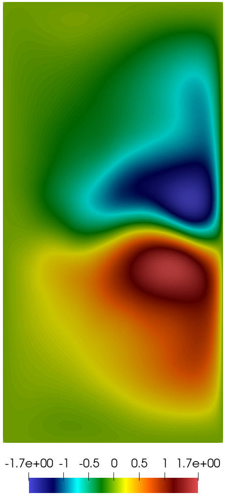
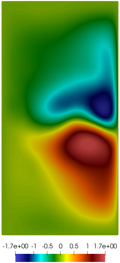
Refer to caption
(a) ψ~1subscript~𝜓1\widetilde{\psi}_{1}, FOM
Refer to caption
(b) ψ~1,q1subscript~𝜓1subscriptsubscript𝑞1\widetilde{\psi}_{1},\mathbf{\mathcal{M}}_{q_{1}}
Refer to caption
(c) ψ~1,ψ1subscript~𝜓1subscriptsubscript𝜓1\widetilde{\psi}_{1},\mathbf{\mathcal{M}}_{\psi_{1}}
Refer to caption
(d) ψ~2subscript~𝜓2\widetilde{\psi}_{2}, FOM
Refer to caption
(e) ψ~2,q2subscript~𝜓2subscriptsubscript𝑞2\widetilde{\psi}_{2},\mathbf{\mathcal{M}}_{q_{2}}
Refer to caption
(f) ψ~2,ψ2subscript~𝜓2subscriptsubscript𝜓2\widetilde{\psi}_{2},\mathbf{\mathcal{M}}_{\psi_{2}}
Figure 19: ψ~1subscript~𝜓1\widetilde{\psi}_{1} (top) and ψ~2subscript~𝜓2\widetilde{\psi}_{2} (bottom) computed over the predictive time interval [50,100]50100[50,100] by the FOM (first column) and the POD-LSTM ROM with modal coefficients from qlsubscriptsubscript𝑞𝑙\mathbf{\mathcal{M}}_{q_{l}} (second column) and ψlsubscriptsubscript𝜓𝑙\mathbf{\mathcal{M}}_{\psi_{l}} (third column).
Model εψl(1)superscriptsubscript𝜀subscript𝜓𝑙1\varepsilon_{\psi_{l}}^{(1)} εψl(2)superscriptsubscript𝜀subscript𝜓𝑙2\varepsilon_{\psi_{l}}^{(2)} Elsubscript𝐸𝑙E_{l} rel. error
ψ1subscript𝜓1\psi_{1} q1subscriptsubscript𝑞1\mathbf{\mathcal{M}}_{q_{1}} 7.838E-02 1.360E-01 9.999E-01
ψ1subscriptsubscript𝜓1\mathbf{\mathcal{M}}_{\psi_{1}} 6.041E-02 1.048E-01 3.642E-01
ψ2subscript𝜓2\psi_{2} q2subscriptsubscript𝑞2\mathbf{\mathcal{M}}_{q_{2}} 4.393E-02 2.597E-01 9.524E-01
ψ1subscriptsubscript𝜓1\mathbf{\mathcal{M}}_{\psi_{1}} 4.543E-02 2.479E-01 2.258E-01
Table 6: Error metrics for time-averaged fields ψ~1subscript~𝜓1\widetilde{\psi}_{1} and ψ~2subscript~𝜓2\widetilde{\psi}_{2}, and kinetic energies E1subscript𝐸1E_{1} and E2subscript𝐸2E_{2} computed by POD-LSTM models qlsubscriptsubscript𝑞𝑙\mathbf{\mathcal{M}}_{q_{l}} and ψlsubscriptsubscript𝜓𝑙\mathbf{\mathcal{M}}_{\psi_{l}} with respect to the FOM computed ψ~lsubscript~𝜓𝑙\widetilde{\psi}_{l} and Elsubscript𝐸𝑙E_{l}.

All the simulations presented in this section were performed on a computing server running a 64-bit version of Linux with a Xeon® processor and 128GB of RAM. A FOM simulation with the parameters specified in (44) over the time interval [10,100]10100[10,100] takes a total of 8.58.58.5 days to complete. The online phase of our POD-LSTM ROM with Nqlr=Nψlr=10superscriptsubscript𝑁subscript𝑞𝑙𝑟superscriptsubscript𝑁subscript𝜓𝑙𝑟10N_{q_{l}}^{r}=N_{\psi_{l}}^{r}=10 and σL=10subscript𝜎𝐿10\sigma_{L}=10 takes 0.5 s for q1subscript𝑞1q_{1}, 0.7 s for q2subscript𝑞2q_{2}, 0.9 s for ψ1subscript𝜓1\psi_{1} and ψ2subscript𝜓2\psi_{2}. This is more than 1E+07 computational speed up compared to the FOM simulation. However, for the offline phase of the ROM, we need to collect the fluctuation field snapshots over the time interval [10,50]1050[10,50] from the FOM and this takes around 3.7 days. Additionally, the training of the LSTM networks ΦsubscriptΦ\mathbf{\mathcal{M}}_{\Phi} takes 58 s for q1subscript𝑞1q_{1}, 59 s for q2subscript𝑞2q_{2}, 61 s for ψ1subscript𝜓1\psi_{1}, and 55 s for ψ2subscript𝜓2\psi_{2}. Both the snapshot collection and the LSTM training only need to be performed once. Lastly, we emphasize that the training of the networks and the online phase for each variable are independent of each other. This means that it is possible to compute the modal coefficients for the variables in parallel.

5.2 Parametric study

While the case of time as the only parameter is interesting in its own right and has allowed us to learn about the advantages and limitations of the POD-LSTM ROM, it is in a parametric study (i.e., a study where physical parameters are varied) that a ROM can show all of its potential. For this reason, we will consider δ𝛿\delta as a variable parameter. All the other parameters are fixed and set as in (44).

We choose to train the POD-LSTM ROM with the following values: δ=0.1,0.3,0.5,0.7,0.9𝛿0.10.30.50.70.9\delta=0.1,0.3,0.5,0.7,0.9. Note that δ=0.5𝛿0.5\delta=0.5 is case considered in Sec. 5.1. To test the prediction capability of the POD-LSTM ROM, we test it for δ=0.125𝛿0.125\delta=0.125 and predict the time-averaged fields q~l,ψ~lsubscript~𝑞𝑙subscript~𝜓𝑙\widetilde{q}_{l},\widetilde{\psi}_{l} over the time interval [50,100]50100[50,100], kinetic energies Elsubscript𝐸𝑙E_{l} (48) and enstrophies lsubscript𝑙\mathcal{E}_{l} (47), for both layers l𝑙l. To build the POD basis, we collect 401 fluctuation snapshots for each training parameter set over the time interval [10,50]1050[10,50] for a total of 2005 fluctuation snapshots for each field of interest. See Fig. 20 for the visualization of training and testing data used in this section. For the LSTM network, we keep the lookback window constant (σL=10subscript𝜎𝐿10\sigma_{L}=10) and use the same hyperparameters specified in Table 1.
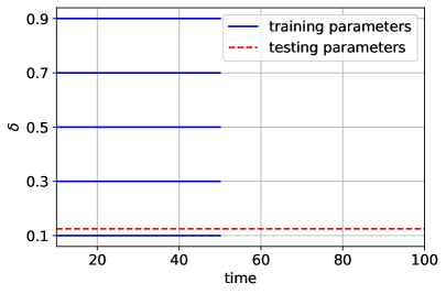
Refer to caption
Figure 20: Parametric study: Training and testing parameters to assess the predictive capabilities of the POD-LSTM ROM.

Let us start by investigating the effect of NΦrsuperscriptsubscript𝑁Φ𝑟N_{\Phi}^{r} on the ROM prediction for the testing parameter δ=0.125𝛿0.125\delta=0.125. The closest sample to δ=0.125𝛿0.125\delta=0.125 is obviously δ=0.1𝛿0.1\delta=0.1, so we set 𝝁c=0.1subscript𝝁𝑐0.1{\mbox{\boldmath{$\mu$}}}_{c}=0.1 in (42). Fig. 21 compares q~lsubscript~𝑞𝑙\widetilde{q}_{l}, l=1,2𝑙12l=1,2, computed by the FOM for δ=0.125𝛿0.125\delta=0.125 with its ROM counterpart for Nqlr=2,4,8,10superscriptsubscript𝑁subscript𝑞𝑙𝑟24810N_{q_{l}}^{r}=2,4,8,10. We see that q~2subscript~𝑞2\widetilde{q}_{2} is rather well reconstructed by the ROM for all Nq2rsuperscriptsubscript𝑁subscript𝑞2𝑟N_{q_{2}}^{r}, while the quality of the reconstruction of q~1subscript~𝑞1\widetilde{q}_{1} varies as Nq1rsuperscriptsubscript𝑁subscript𝑞1𝑟N_{q_{1}}^{r} changes. Towards the basin center, q~1subscript~𝑞1\widetilde{q}_{1} exhibits a thin oscillating transition layer which is captured when Nq1r=4superscriptsubscript𝑁subscript𝑞1𝑟4N_{q_{1}}^{r}=4 and Nq1r=10superscriptsubscript𝑁subscript𝑞1𝑟10N_{q_{1}}^{r}=10, but not when Nq1r=2superscriptsubscript𝑁subscript𝑞1𝑟2N_{q_{1}}^{r}=2 or Nq1r=8superscriptsubscript𝑁subscript𝑞1𝑟8N_{q_{1}}^{r}=8. We also observe that the small negative values (cyan region) is better captured as we increase Nq1rsuperscriptsubscript𝑁subscript𝑞1𝑟N_{q_{1}}^{r}, with Nq1r=10superscriptsubscript𝑁subscript𝑞1𝑟10N_{q_{1}}^{r}=10 giving the solution that compares more favorably with the FOM solution. This is also supported by the error metrics εq1(1)superscriptsubscript𝜀subscript𝑞11\varepsilon_{q_{1}}^{(1)} (45) and εq1(2)superscriptsubscript𝜀subscript𝑞12\varepsilon_{q_{1}}^{(2)} (46) reported in Table 7. Although Nq2r=10superscriptsubscript𝑁subscript𝑞2𝑟10N_{q_{2}}^{r}=10 does not provide the lowest error in either metric, all the values are comparable and it gives the smallest relative L2superscript𝐿2L^{2} error for the enstrophy in the bottom layer.

FOM Nqlr=2superscriptsubscript𝑁subscript𝑞𝑙𝑟2N_{q_{l}}^{r}=2 Nqlr=4superscriptsubscript𝑁subscript𝑞𝑙𝑟4N_{q_{l}}^{r}=4 Nqlr=8superscriptsubscript𝑁subscript𝑞𝑙𝑟8N_{q_{l}}^{r}=8 Nqlr=10superscriptsubscript𝑁subscript𝑞𝑙𝑟10N_{q_{l}}^{r}=10
q~1subscript~𝑞1\widetilde{q}_{1} Refer to caption Refer to caption Refer to caption Refer to caption Refer to caption
q~2subscript~𝑞2\widetilde{q}_{2} Refer to caption Refer to caption Refer to caption Refer to caption Refer to caption
Figure 21: Parametric study: Time-averaged vorticities q~1subscript~𝑞1\widetilde{q}_{1} (top) and q~2subscript~𝑞2\widetilde{q}_{2} (bottom) over the predictive time interval [50,100]50100[50,100] computed by FOM (first column) and POD-LSTM ROM with Nqlr=2,4,8,10superscriptsubscript𝑁subscript𝑞𝑙𝑟24810N_{q_{l}}^{r}=2,4,8,10 (second to fifth columns)

.

Nq1rsuperscriptsubscript𝑁subscript𝑞1𝑟N_{q_{1}}^{r} δq1subscript𝛿subscript𝑞1\delta_{q_{1}} εq1(1)superscriptsubscript𝜀subscript𝑞11\varepsilon_{q_{1}}^{(1)} εq1(2)superscriptsubscript𝜀subscript𝑞12\varepsilon_{q_{1}}^{(2)} 1subscript1\mathcal{E}_{1} rel. err.
2 0.03 3.195E-01 3.099E-01 2.296E-01
4 0.04 2.427E-01 2.354E-01 1.863E-01
8 0.07 3.092E-01 2.998E-01 2.791E-01
10 0.08 2.025E-01 1.965E-01 1.873E-01
Nq2rsuperscriptsubscript𝑁subscript𝑞2𝑟N_{q_{2}}^{r} δq2subscript𝛿subscript𝑞2\delta_{q_{2}} εq2(1)superscriptsubscript𝜀subscript𝑞21\varepsilon_{q_{2}}^{(1)} εq2(2)superscriptsubscript𝜀subscript𝑞22\varepsilon_{q_{2}}^{(2)} 2subscript2\mathcal{E}_{2} rel. err.
2 0.04 1.437E-02 2.706E-02 3.421E-02
4 0.06 1.421E-02 2.675E-02 2.932E-02
8 0.09 1.496E-02 2.818E-02 2.819E-02
10 0.10 1.524E-02 2.869E-02 2.599E-02
Table 7: Parametric study: fraction of retained eigenvalue energy δqlsubscript𝛿subscript𝑞𝑙\delta_{q_{l}}, error metrics εql(1)superscriptsubscript𝜀subscript𝑞𝑙1\varepsilon_{q_{l}}^{(1)} (45) and εql(2)superscriptsubscript𝜀subscript𝑞𝑙2\varepsilon_{q_{l}}^{(2)} (46), and relative L2superscript𝐿2L^{2} error for enstrophy lsubscript𝑙\mathcal{E}_{l} (47), l=1,2𝑙12l=1,2, for different numbers of POD modes retained.

Next, let us look at the reconstruction of ψ~lsubscript~𝜓𝑙\widetilde{\psi}_{l}, l=1,2𝑙12l=1,2, when Nψlrsuperscriptsubscript𝑁subscript𝜓𝑙𝑟N_{\psi_{l}}^{r} varies in Fig. 22. Note that in the top layer there are two large and irregularly shaped gyes, while the large gyres are lost in the bottom layer. The ROM predictions of ψ~1subscript~𝜓1\widetilde{\psi}_{1} match well with the ψ~1subscript~𝜓1\widetilde{\psi}_{1} given by the FOM for all Nψ1rsuperscriptsubscript𝑁subscript𝜓1𝑟N_{\psi_{1}}^{r}. We see that Nψ1r=2superscriptsubscript𝑁subscript𝜓1𝑟2N_{\psi_{1}}^{r}=2 predicts the shape of the red gyre (large positive values) in the Southern region of the ocean basin most accurately but Nψ1r=10superscriptsubscript𝑁subscript𝜓1𝑟10N_{\psi_{1}}^{r}=10 is able to capture the blue gyre (large negative values) in the Northern region better than the rest of the cases considered. In fact, Nψ1r=10superscriptsubscript𝑁subscript𝜓1𝑟10N_{\psi_{1}}^{r}=10 results into the lowest error metrics εψl(1)superscriptsubscript𝜀subscript𝜓𝑙1\varepsilon_{\psi_{l}}^{(1)} (45) and εψl(2)superscriptsubscript𝜀subscript𝜓𝑙2\varepsilon_{\psi_{l}}^{(2)} (46), as reported in the third and fourth columns of Table 8. The results for ψ~2subscript~𝜓2\widetilde{\psi}_{2} differ significantly when Nψ2rsuperscriptsubscript𝑁subscript𝜓2𝑟N_{\psi_{2}}^{r} is varied. We see that Nψ2r=2superscriptsubscript𝑁subscript𝜓2𝑟2N_{\psi_{2}}^{r}=2 and Nψ2r=8superscriptsubscript𝑁subscript𝜓2𝑟8N_{\psi_{2}}^{r}=8 cannot accurately capture the time-averaged dynamics in the lower layer, especially around the center of the basin and in the Southern region. On the other hand, the ROM prediction improves when Nψ2r=4superscriptsubscript𝑁subscript𝜓2𝑟4N_{\psi_{2}}^{r}=4, and even more when Nψ2r=10superscriptsubscript𝑁subscript𝜓2𝑟10N_{\psi_{2}}^{r}=10. These observations are reflected in the root mean square error εψ2(1)superscriptsubscript𝜀subscript𝜓21\varepsilon_{\psi_{2}}^{(1)} (45) and the L2superscript𝐿2L^{2} relative error εψ2(2)superscriptsubscript𝜀subscript𝜓22\varepsilon_{\psi_{2}}^{(2)} (46) in the third and fourth columns of Table 8. Table 8 also reports the relative error for the predicted time-evolution of the kinetic energy Elsubscript𝐸𝑙E_{l}. We see that the errors are comparable across all values of Nψlrsuperscriptsubscript𝑁subscript𝜓𝑙𝑟N_{\psi_{l}}^{r}.

FOM Nψlr=2superscriptsubscript𝑁subscript𝜓𝑙𝑟2N_{\psi_{l}}^{r}=2 Nψlr=4superscriptsubscript𝑁subscript𝜓𝑙𝑟4N_{\psi_{l}}^{r}=4 Nψlr=8superscriptsubscript𝑁subscript𝜓𝑙𝑟8N_{\psi_{l}}^{r}=8 Nψlr=10superscriptsubscript𝑁subscript𝜓𝑙𝑟10N_{\psi_{l}}^{r}=10
ψ~1subscript~𝜓1\widetilde{\psi}_{1} Refer to caption Refer to caption Refer to caption Refer to caption Refer to caption
ψ~2subscript~𝜓2\widetilde{\psi}_{2} Refer to caption Refer to caption Refer to caption Refer to caption Refer to caption
Figure 22: Parametric study: Time-averaged stream functions ψ~1subscript~𝜓1\widetilde{\psi}_{1} (top) and ψ~2subscript~𝜓2\widetilde{\psi}_{2} (bottom) over the predictive time interval [50,100]50100[50,100] computed by FOM (first column) and POD-LSTM ROM with Nψlr=2,4,8,10superscriptsubscript𝑁subscript𝜓𝑙𝑟24810N_{\psi_{l}}^{r}=2,4,8,10 (second to fifth columns)

.

Nψ1rsuperscriptsubscript𝑁subscript𝜓1𝑟N_{\psi_{1}}^{r} δψ1subscript𝛿subscript𝜓1\delta_{\psi_{1}} εψ1(1)superscriptsubscript𝜀subscript𝜓11\varepsilon_{\psi_{1}}^{(1)} εψ1(2)superscriptsubscript𝜀subscript𝜓12\varepsilon_{\psi_{1}}^{(2)} E1subscript𝐸1E_{1} rel. err.
2 0.31 1.398E-01 2.027E-01 7.151E-01
4 0.40 1.336E-01 1.937E-01 7.129E-01
8 0.50 1.339E-01 1.940E-01 7.171E-01
10 0.54 1.282E-01 1.855E-01 7.189E-01
Nψ2rsuperscriptsubscript𝑁subscript𝜓2𝑟N_{\psi_{2}}^{r} δψ2subscript𝛿subscript𝜓2\delta_{\psi_{2}} εψ2(1)superscriptsubscript𝜀subscript𝜓21\varepsilon_{\psi_{2}}^{(1)} εψ2(2)superscriptsubscript𝜀subscript𝜓22\varepsilon_{\psi_{2}}^{(2)} E2subscript𝐸2E_{2} rel. err.
2 0.37 5.923E-02 1.731E+00 9.561E-01
4 0.49 2.561E-02 7.485E-01 9.643E-01
8 0.61 4.253E-02 1.243E+00 9.571E-01
10 0.65 1.887E-02 5.513E-01 9.647E-01
Table 8: Parametric study: fraction of retained eigenvalue energy δψlsubscript𝛿subscript𝜓𝑙\delta_{\psi_{l}}, error metrics εψl(1)superscriptsubscript𝜀subscript𝜓𝑙1\varepsilon_{\psi_{l}}^{(1)} (45) and εψl(2)superscriptsubscript𝜀subscript𝜓𝑙2\varepsilon_{\psi_{l}}^{(2)} (46), and relative L2superscript𝐿2L^{2} error for kinetic energy Elsubscript𝐸𝑙E_{l} (47), l=1,2𝑙12l=1,2, for different numbers of POD modes retained.

Next, we show the absolute difference between the true time-averaged fields coming from the FOM and the POD-LSTM ROM with NΦr=10superscriptsubscript𝑁Φ𝑟10N_{\Phi}^{r}=10 and σL=10subscript𝜎𝐿10\sigma_{L}=10 in Fig. 23. We see that the peaks in the absolute difference are localized. Notice that although it might seem that for q~2subscript~𝑞2\widetilde{q}_{2}, there is a large red region, i.e., large absolute difference, the maximum absolute difference is of order 1E-02.
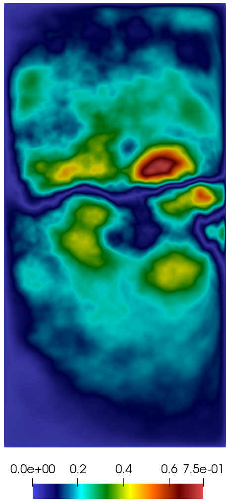
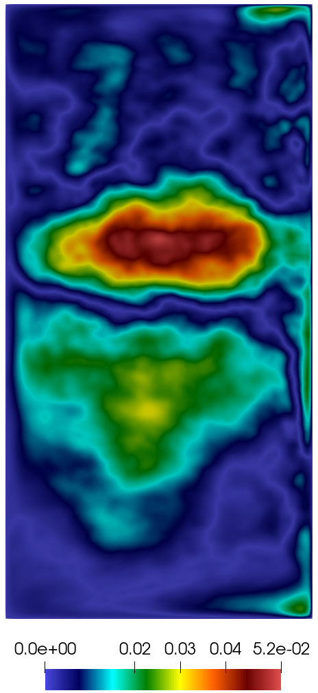
Refer to caption
(a) |q~1FOMq~1ROM|superscriptsubscript~𝑞1FOMsuperscriptsubscript~𝑞1ROM\absolutevalue{\widetilde{q}_{1}^{\text{FOM}}-\widetilde{q}_{1}^{\text{ROM}}}
Refer to caption
(b) |q~2FOMq~2ROM|superscriptsubscript~𝑞2FOMsuperscriptsubscript~𝑞2ROM\absolutevalue{\widetilde{q}_{2}^{\text{FOM}}-\widetilde{q}_{2}^{\text{ROM}}}
Refer to caption
(c) |ψ~1FOMψ~1ROM|superscriptsubscript~𝜓1FOMsuperscriptsubscript~𝜓1ROM\absolutevalue{\widetilde{\psi}_{1}^{\text{FOM}}-\widetilde{\psi}_{1}^{\text{ROM}}}
Refer to caption
(d) |ψ~2FOMψ~2ROM|superscriptsubscript~𝜓2FOMsuperscriptsubscript~𝜓2ROM\absolutevalue{\widetilde{\psi}_{2}^{\text{FOM}}-\widetilde{\psi}_{2}^{\text{ROM}}}
Figure 23: Parametric study: Absolute difference between the FOM time-averaged solutions and the predicted time-averaged fields computed by the POD-LSTM ROM with NΦr=10superscriptsubscript𝑁Φ𝑟10N_{\Phi}^{r}=10 and σL=10subscript𝜎𝐿10\sigma_{L}=10.
Remark 5.1.

In the case of δ=0.125𝛿0.125\delta=0.125, it was obvious to take 𝛍c=0.1subscript𝛍𝑐0.1{\mbox{\boldmath{$\mu$}}}_{c}=0.1 in (42). However, if one is interested in the ROM approximation for δ=0.2𝛿0.2\delta=0.2 with the sampling in Fig. 20, the choice between 𝛍c=0.1subscript𝛍𝑐0.1{\mbox{\boldmath{$\mu$}}}_{c}=0.1 and 𝛍c=0.3subscript𝛍𝑐0.3{\mbox{\boldmath{$\mu$}}}_{c}=0.3 is less obvious. We found out that the time-averaged FOM fields for δ=0.2𝛿0.2\delta=0.2 are much closer to the time-averaged fields for δ=0.1𝛿0.1\delta=0.1 than δ=0.3𝛿0.3\delta=0.3 and, hence, 𝛍c=0.1subscript𝛍𝑐0.1{\mbox{\boldmath{$\mu$}}}_{c}=0.1 yields a more accurate ROM approximation for δ=0.2𝛿0.2\delta=0.2. A more robust ROM approximation could be obtained by replacing q~l0superscriptsubscript~𝑞𝑙0\widetilde{q}_{l}^{0} and ψ~l0superscriptsubscript~𝜓𝑙0\widetilde{\psi}_{l}^{0} in (25)-(26) with higher order approximations of q~l(𝐱,𝛍)subscript~𝑞𝑙𝐱𝛍\widetilde{q}_{l}(\boldsymbol{x},\mbox{\boldmath{$\mu$}}) and ψ~l(𝐱,𝛍)subscript~𝜓𝑙𝐱𝛍\widetilde{\psi}_{l}(\boldsymbol{x},\mbox{\boldmath{$\mu$}}).

To conclude this section, we comment on the computational time savings. All simulations were carried out using the same machine described in Sec. 5.1. For the offline phase of the parametric study, we need to collect the fluctuation field snapshots over the time interval [10,50]1050[10,50] from the FOM for five values of δ𝛿\delta. Each of such FOM simulations takes around 3.7 days, so the offline phase is significantly more expensive if not run in parallel. The corresponding ROM computations online, with Nqlr=Nψlr=10superscriptsubscript𝑁subscript𝑞𝑙𝑟superscriptsubscript𝑁subscript𝜓𝑙𝑟10N_{q_{l}}^{r}=N_{\psi_{l}}^{r}=10 modes retained and lookback window of σL=10subscript𝜎𝐿10\sigma_{L}=10, take 0.51 s for both q1subscript𝑞1q_{1} and q2subscript𝑞2q_{2}, 0.52 s for ψ1subscript𝜓1\psi_{1}, and 0.55 s for ψ2subscript𝜓2\psi_{2}.

6 Conclusions

We proposed a POD-based data-driven ROM to capture the large-scale behavior of ocean dynamics described by the two-layer quasi-geostrophic equations. The ROM approximates the solution of the 2QGE with a linear combination of POD modes, with modal coefficients found through a recurrent neural network called long short-term memory. The LSTM architecture was chosen for its robustness and stability in predicting chaotic dynamical systems. The proposed methodology consists of two phases: offline and online. During the offline phase, snapshots data are collected from a high-resolution simulation for a given time interval (and given parameter values, in the case of variable physical parameters), the reduced basis for each field variable is generated via POD, and the LSTM architecture is trained with the time-dependent modal coefficients associated with the snapshots. A critical model parameter to set in this phase is the lookback window for the LSTM, i.e., the quantity that tells the network how far in the past to look. During the online phase, the trained model is used to predict the modal coefficients recursively for the remaining of the time interval of interest (and new parameter values, in the case of variable physical parameters).

We assessed the performance of the POD-LSTM ROM with an extension of a widely used benchmark called the double-gyre wind forcing experiment. We started by considering time as the only parameter and then included the the aspect ratio δ𝛿\delta between the two ocean layers as a variable parameter. Our results indicate that, even when retaining only 1020%10percent2010-20\% of the singular value energy of the system, our POD-LSTM ROM provides an accurate prediction of both time-averaged fields and time-dependent quantities (modal coefficients, enstrophy, and kinetic energy). We observe up to 1E+07 computational speed up in the online phase compared to the FOM. A drawback of this approach is its sensitivity to the lookback window. Our computational study indicates there is an “optimal value”, past which the prediction by the POD-LSTM ROM degenerates. Once this sensitivity is better understood, the POD-LSTM ROM will be a methodology, not only accurate and efficient, but also robust for the prediction of large-scale flows with choatic spatio-temporal behavior.

Acknowledgements

We acknowledge the support provided by PRIN “FaReX - Full and Reduced order modelling of coupled systems: focus on non-matching methods and automatic learning” project, PNRR NGE iNEST “Interconnected Nord-Est Innovation Ecosystem” project, INdAM-GNCS 2019–2020 projects and PON “Research and Innovation on Green related issues” FSE REACT-EU 2021 project. This work was also partially supported by the U.S. National Science Foundation through Grant No. DMS-1953535 (PI A. Quaini).

References

  • [1] J. Weller, E. Lombardi, M. Bergmann, A. Iollo, Numerical methods for low-order modeling of fluid flows based on POD, International Journal for Numerical Methods in Fluids 63 (2010) 249–268.
  • [2] S. Giere, Numerical and analytical aspects of pod-based reduced-order modeling in computational fluid dynamics, Ph.D. thesis, Freien Universität Berlin (2016).
  • [3] M. Girfoglio, A. Quaini, G. Rozza, A POD-Galerkin reduced order model for a LES filtering approach, Journal of Computational Physics 436 (2021) 110260.
  • [4] D. Xiao, F. Fang, C. Pain, G. Hu, Non-intrusive reduced-order modelling of the Navier–Stokes equations based on RBF interpolation, International Journal for Numerical Methods in Fluids 79 (2015) 580–595.
  • [5] R. Maulik, A. Mohan, B. Lusch, S. Madireddy, P. Balaprakash, D. Livescu, Time-series learning of latent-space dynamics for reduced-order model closure, Physica D: Nonlinear Phenomena 405 (2020) 132368.
  • [6] F. Casenave, N. Akkari, F. Bordeu, C. Rey, D. Ryckelynck, A nonintrusive distributed reduced-order modeling framework for nonlinear structural mechanics—Application to elastoviscoplastic computations, International Journal for Numerical Methods in Engineering 121 (2019) 32–53.
  • [7] M. Guo, J. S. Hesthaven, Reduced order modeling for nonlinear structural analysis using Gaussian process regression, Computer Methods in Applied Mechanics and Engineering 341 (2018) 807–826.
  • [8] R. Lin, M. Lim, Structural sensitivity analysis via reduced-order analytical model, Computer Methods in Applied Mechanics and Engineering 121 (1995) 345–359.
  • [9] J. Oliver, M. Caicedo, A. Huespe, J. Hernández, E. Roubin, Reduced order modeling strategies for computational multiscale fracture, Computer Methods in Applied Mechanics and Engineering 313 (2017) 560–595.
  • [10] S. Fresca, A. Manzoni, L. Dede, A. Quarteroni, POD-enhanced deep learning-based reduced order models for the real-time simulation of cardiac electrophysiology in the left atrium, Front. Physiol. 12 (2021) 679076.
  • [11] S. Fresca, A. Manzoni, L. Dede, A. Quarteroni, Deep learning-based reduced order models in cardiac electrophysiology, PLoS ONE 15 (2020) e0239416.
  • [12] M. R. Pfaller, M. C. Varona, C. B. J. Lang, W. A. Wall, Using parametric model order reduction for inverse analysis of large nonlinear cardiac simulations, International Journal for Numerical Methods in Biomedical Engineering 36 (2020) e3320.
  • [13] L. O. Müller, A. Caiazzo, P. J. Blanco, Reduced-Order Unscented Kalman Filter With Observations in the Frequency Domain: Application to Computational Hemodynamics, IEEE Transactions on Biomedical Engineering 66 (2019) 1269–1276.
  • [14] M. Tezzele, F. Ballarin, G. Rozza, Combined Parameter and Model Reduction of Cardiovascular Problems by Means of Active Subspaces and POD-Galerkin Methods, Springer International Publishing, Cham, 2018, pp. 185–207.
  • [15] F. Ballarin, E. Faggiano, S. Ippolito, A. Manzoni, A. Quarteroni, G. Rozza, R. Scrofani, Fast simulations of patient-specific haemodynamics of coronary artery bypass grafts based on a POD-Galerkin method and a vascular shape parametrization, Journal of Computational Physics 315 (2016) 609 – 628. doi:https://doi.org/10.1016/j.jcp.2016.03.065.
    URL http://www.sciencedirect.com/science/article/pii/S0021999116300304
  • [16] M. Tezzele, N. Demo, A. Mola, G. Rozza, An integrated data-driven computational pipeline with model order reduction for industrial and applied mathematics, Springer International Publishing, Cham, 2022, pp. 179–200. doi:10.1007/978-3-030-96173-2_7.
    URL https://doi.org/10.1007/978-3-030-96173-2_7
  • [17] M. Gadalla, M. Cianferra, M. Tezzele, G. Stabile, A. Mola, G. Rozza, On the comparison of LES data-driven reduced order approaches for hydroacoustic analysis, Computers & Fluids 216 (2021) 104819. doi:https://doi.org/10.1016/j.compfluid.2020.104819.
    URL https://www.sciencedirect.com/science/article/pii/S0045793020303893
  • [18] N. Demo, M. Tezzele, A. Mola, G. Rozza, Hull shape design optimization with parameter space and model reductions, and self-learning mesh morphing, Journal of Marine Science and Engineering 9 (2) (2021). doi:10.3390/jmse9020185.
    URL https://www.mdpi.com/2077-1312/9/2/185
  • [19] M. Tezzele, F. Salmoiraghi, A. Mola, G. Rozza, Dimension reduction in heterogeneous parametric spaces with application to naval engineering shape design problems, Adv. Model. and Simul. in Eng. Sci. 5 (2018) 1–19.
  • [20] B. Peter, S. Grivet-Talocia, Q. Alfio, R. Gianluigi, S. Wil, L. M. Silveira, et al., Model Order Reduction. Volume 1: System-and Data-Driven Methods and Algorithms, De Gruyter, Berlin, Boston, 2021. doi:doi:10.1515/9783110498967.
  • [21] P. Benner, W. Schilders, S. Grivet-Talocia, A. Quarteroni, G. Rozza, L. Miguel Silveira, Model Order Reduction: Volume 2: Snapshot-Based Methods and Algorithms, De Gruyter, 2020.
  • [22] P. Benner, W. Schilders, S. Grivet-Talocia, A. Quarteroni, G. Rozza, L. Miguel Silveira, Model order reduction: volume 3 applications, De Gruyter, 2020.
  • [23] J. S. Hesthaven, G. Rozza, B. Stamm, Certified reduced basis methods for parametrized partial differential equations, Vol. 590, Springer, 2016.
  • [24] M. H. Malik, Reduced Order Modeling for smart grids’ simulation and optimization, Ph.D. thesis, École centrale de Nantes; Universitat politécnica de Catalunya (2017).
  • [25] G. Rozza, D. B. P. Huynh, A. T. Patera, Reduced basis approximation and a posteriori error estimation for affinely parametrized elliptic coercive partial differential equations: application to transport and continuum mechanics, Archives of Computational Methods in Engineering 15 (3) (2008) 229–275.
  • [26] G. Rozza, G. Stabile, F. Ballarin, Advanced Reduced Order Methods and Applications in Computational Fluid Dynamics, Society for Industrial and Applied Mathematics, 2022.
  • [27] O. San, T. Iliescu, A stabilized proper orthogonal decomposition reduced-order model for large scale quasigeostrophic ocean circulation, Advances in Computational Mathematics 41 (2015) 1289–1319.
  • [28] C. Mou, H. Liu, D. Wells, T. Iliescu, Data-driven correction reduced order models for the quasi-geostrophic equations: a numerical investigation, International Journal of Computational Fluid Dynamics 34 (2020) 147–159.
  • [29] S. M. Rahman, O. San, A. Rasheed, A hybrid approach for model order reduction of barotropic quasi-geostrophic turbulence, Fluids 3 (2018) 86.
  • [30] S. M. Rahman, S. Pawar, O. San, T. Iliescu, Nonintrusive reduced order modeling framework for quasigeostrophic turbulence, Physical Review E 100 (2019) 053306.
  • [31] J. N. Kutz, S. L. Brunton, B. W. Brunton, J. L. Proctor, Dynamic Mode Decomposition: data-driven modeling of complex systems, SIAM, 2016.
  • [32] M. Golzar, M. K. Moayyedi, F. Fotouhi, A surrogate non-intrusive reduced order model of quasi-geostrophic turbulence dynamics based on a combination of lstm and different approaches of dmd, Journal of Turbulence 24 (2023) 474–505.
  • [33] D. Qi, A. Majda, Low-Dimensional Reduced-Order Models for Statistical Response and Uncertainty Quantification: Two-Layer Baroclinic Turbulence, Journal of the Atmospheric Sciences 73 (12) (2016) 4609–4639.
  • [34] J. Marshall, C. Hill, L. Perelman, A. Adcroft, Hydrostatic, quasi-hydrostatic, and nonhydrostatic ocean modeling, Journal of Geophysical Research: Oceans 102 (C3) (1997) 5733–5752. doi:https://doi.org/10.1029/96JC02776.
  • [35] T. M. Ozgokmen, E. P. Chassignet, Emergence of inertial gyres in a two-layer quasigeostrophic ocean model, Journal of Physical Oceanography 28 (3) (1998) 461 – 484. doi:10.1175/1520-0485(1998)028<0461:EOIGIA>2.0.CO;2.
  • [36] P. S. Berloff, J. C. McWilliams, Large-scale, low-frequency variability in wind-driven ocean gyres, Journal of Physical Oceanography 29 (8) (1999) 1925 – 1949. doi:10.1175/1520-0485(1999)029<1925:LSLFVI>2.0.CO;2.
  • [37] M. DiBattista, A. Majda, Equilibrium statistical predictions for baroclinic vortices: The role of angular momentum, Theoret. Comput. Fluid Dynamics 14 (2001) 293–322.
  • [38] P. Berloff, I. Kamenovich, J. Pedlosky, A mechanism of formation of multiple zonal jets in the oceans, Journal of Fluid Mechanics 628 (2009) 395–425. doi:10.1017/S0022112009006375.
  • [39] L. Besabe, M. Girfoglio, A. Quaini, G. Rozza, Linear and nonlinear filtering for a two-layer quasi-geostrophic ocean model, https://arxiv.org/abs/2404.11718 (2024).
  • [40] O. San, A. Staples, T. Iliescu, Approximate deconvolution large eddy simulation of a stratified two-layer quasigeostrophic ocean model, Ocean Modelling 63 (2012) 1–20.
  • [41] R. Salmon, Two-layer quasi-geostrophic turbulence in a simple special case, Geophysical & Astrophysical Fluid Dynamics 10 (1978) 25–52.
  • [42] T. T. Medjo, Numerical simulations of a two-layer quasi-geostrophic equation of the ocean, SIAM Journal of Numerical Analysis 37 (2000) 2005–2022.
  • [43] C. B. Fandry, L. M. Leslie, A two-layer quasi-geostrophic model of summer trough formation in the australian subtropical easterlies, Journal of the Atmospheric Sciences 41 (1984) 807–818.
  • [44] M. Mu, Z. Qingcun, T. G. Shepherd, L. Yongming, Nonlinear stability of multilayer quasi-geostrophic flow, Journal of Fluid Dynamics 264 (1994) 165–184.
  • [45] M. Girfoglio, A. Quaini, G. Rozza, A novel large eddy simulation model for the quasi-geostrophic equations in a finite volume setting, Journal of Computational and Applied Mathematics 418 (2023) 114656.
  • [46] M. Girfoglio, A. Quaini, G. Rozza, A Finite Volume approximation of the Navier-Stokes equations with nonlinear filtering stabilization, Computers & Fluids 187 (2019) 27–45.
  • [47] M. Girfoglio, A. Quaini, G. Rozza, A POD-Galerkin reduced order model for the Navier-Stokes equations in stream function-vorticity formulation, Computers & Fluids 244 (2022) 105536.
  • [48] GEA - Geophysical and Environmental Applications, https://github.com/GEA-Geophysical-and-Environmental-Apps/GEA (2023).
  • [49] M. Girfoglio, A. Quaini, G. Rozza, GEA: A New Finite Volume-Based Open Source Code for the Numerical Simulation of Atmospheric and Ocean Flows, in: Finite Volumes for Complex Applications X—Volume 2, Hyperbolic and Related Problems, 2023, pp. 151–159.
  • [50] H. G. Weller, G. Tabor, H. Jasak, C. Fureby, A tensorial approach to computational continuum mechanics using object-oriented techniques, Computers in physics 12 (1998) 620–631.
  • [51] E. A. Christensen, M. Brøns, J. N. Sørensen, Evaluation of Proper Orthogonal Decomposition–Based Decomposition Techniques Applied to Parameter-Dependent Nonturbulent Flows, SIAM Journal on Scientific Computing 21 (1999) 1419–1434.
  • [52] A. Chatterjee, An introduction to the proper orthogonal decomposition, Current Science 78 (2000) 808–817.
  • [53] K. Kunisch, S. Volkwein, Galerkin proper orthogonal decomposition methods for a general equation in fluid dynamics, SIAM Journal on Numerical Analysis 40 (2003) 492–515.
  • [54] M. Sieber, C. O. Paschereit, K. Oberleithner, Spectral proper orthogonal decomposition, Journal of Fluid Mechanics 792 (2016) 798–828.
  • [55] C. Mou, Z. Wang, D. Wells, X. Xie, T. Iliescu, Reduced order models for the quasi-geostrophic equations: A brief survey, Fluids 6 (2020) 16.
  • [56] Z. Wang, D. Xiao, F. Fang, R. Govindan, C. Pain, Y. Guo, Model identification of reduced order fluid dynamics systems using deep learning, International Journal for Numerical Methods in Fluids 86 (2018) 4.
  • [57] S. Hochreiter, J. Schmidhuber, Long Short-Term Memory, Neural Computation 9 (1997) 1735–1780.
  • [58] Y. Bengio, P. Simard, P. Frasconi, Learning long-term dependencies with gradient descent is difficult, IEEE Transactions on Neural Networks 5 (1994) 157–166.
  • [59] J. Bayer, Learning sequence representation, Ph.D. thesis, Technische Universität München (2015).
  • [60] A. Sherstinsky, Fundamentals of Recurrent Neural Network (RNN) and Long Short-Term Memory (LSTM) network, Physica D: Nonlinear Phenomena 404 (2020) 132306.
  • [61] B. Nadiga, L. Margolin, Dispersive-dissipative eddy parameterization in a barotropic model, Journal of Physical Oceanography 31 (2001) 2525–2531.
  • [62] D. Holm, B. Nadiga, Modeling mesoscale turbulence in the barotropic double-gyre circulation, Journal of Physical Oceanography 33 (2003) 2355–2365.
  • [63] R. Greatbatch, B. Nadiga, Four-gyre circulation in a barotropic model with double-gyre wind forcing, Journal of Physical Oceanography 30 (2000) 1461–1471.
  • [64] I. Monteiro, C. Carolina, Improving numerical accuracy in a regularized barotropic vorticity model of geophysical flow, International Journal of Numerical Analysis and Modelling, Series B 5 (2014) 317–338.
  • [65] I. Monteiro, C. Manica, L. Rebholz, Numerical study of a regularized barotropic vorticity model of geophysical flow, Numerical Methods for Partial Differential Equations 31 (2015) 1492–1514.
  • [66] Z. Mou, C.and Wang, D. Wells, X. Xie, T. Iliescu, Reduced order models for the quasi-geostrophic equations: A brief survey, Fluids 6 (2020) 16. doi:10.3390/fluids6010016.
  • [67] M. Girfoglio, A. Quaini, G. Rozza, A linear filter regularization for POD-based reduced-order models of the quasi-geostrophic equations, Comptes Rendus. Mécanique 351 (2023) 1–21.
  • [68] D. Kingma, J. Ba, Adam: A Method for Stochastic Optimization, https://arxiv.org/abs/1412.6980 (2014).