Hydrogen reaction rate modeling based on convolutional neural network for large eddy simulation

Abstract

This paper establishes a data-driven modeling framework for lean Hydrogen (H₂)-air reaction rates for the Large Eddy Simulation (LES) of turbulent reactive flows. This is particularly challenging since H₂ molecules diffuse much faster than heat, leading to large variations in burning rates, thermodiffusive instabilities at the subfilter scale, and complex turbulence-chemistry interactions. Our data-driven approach leverages a Convolutional Neural Network (CNN), trained to approximate filtered burning rates from emulated LES data. First, five different lean premixed turbulent H₂-air flame Direct Numerical Simulations (DNSs) are computed each with a unique global equivalence ratio. Second, DNS snapshots are filtered and downsampled to emulate LES data. Third, a CNN is trained to approximate the filtered burning rates as a function of LES scalar quantities: progress variable, local equivalence ratio and flame thickening due to filtering. Finally, the performances of the CNN model are assessed on test solutions never seen during training. The model retrieves burning rates with very high accuracy. It is also tested on two filter and downsampling parameters and two global equivalence ratios between those used during training. For these interpolation cases, the model approximates burning rates with low error even though the cases were not included in the training dataset. This a priori study shows that the proposed data-driven machine learning framework is able to address the challenge of modeling lean premixed H₂-air burning rates. It paves the way for a new modeling paradigm for the simulation of carbon-free hydrogen combustion systems.

YEAR

Quentin Malé et al.

Quentin Malé et al.

Impact Statement

Large Eddy Simulation (LES) plays a key role in the design of new combustion chambers for robust and safe combustion of carbon-free fuels such as H₂. It is a very efficient method which consists of filtering and modeling small-scale flow physics that would otherwise be very computationally expensive to resolve. However, the high molecular diffusion of H₂ challenges current subfilter-scale modeling approaches for lean premixed mixtures. By establishing a framework for data-driven machine learning modeling of LES burning rates, this work can enable high-fidelity simulation of hydrogen combustion systems. These combustion systems are essential for achieving a low-carbon economy.

1 Introduction

The urgent need to drastically reduce our greenhouse gas emissions requires us to develop alternative solutions to fossil fuel combustion. Sustainably produced hydrogen (H₂) is a promising energy carrier for the decarbonization of combustion systems where there is no viable technology to be a substitute. This is the case, for example, with gas turbines for power generation or aviation, as well as some industrial burners. However, compared with conventional fuels, H₂-air combustion involves higher flame temperatures, much higher flame speeds, and a very wide flammability range. These characteristics pose considerable challenges for the design of new H₂ combustion devices, ensuring stable, robust and safe operation. In this context, high-fidelity simulation of turbulent combustion plays a key role. It is essential both for a fundamental understanding of flame behavior, and as an aid to the design of industrial combustion devices. It is also crucial for modeling safety scenarios, with hydrogen expected to be widely used to decarbonize industry.

Hydrogen does not only challenge the way combustion chambers should be designed, it also constitutes a key difficulty for our simulation methods. Indeed, H₂ is a very peculiar fuel due to its small Lewis number. Its high molecular diffusion, much faster than heat, gives rise to unique phenomena, especially when burned lean (i.e. with excess air) and premixed. First, lean hydrogen flames are prone to thermodiffusive instabilities. The disparity between heat and H₂ mass fluxes amplifies small flame front perturbations, inducing significant flame wrinkling and strong variations of the reaction rates along the flame front [30, 3, 4]. Second, burning rates increase significantly with the strain rate. With H₂ diffusing faster than heat, the reaction zone moves to the hot gas side of the flame as the strain increases. The reaction rates then increase monotonically with the strain rate, up to the extinction limit [28].

Unfortunately, these phenomena can occur on scales smaller than those that can be resolved numerically. The community nowadays uses Large Eddy Simulation (LES) methods, which involve simulating only the largest flow structures, to compute real complex configurations at an affordable computing cost. The smaller scales are modeled, according to Subgrid-Scale (SGS) models [30], also called subfilter-scale models. The complexity of these phenomena, specific to H₂, poses many challenges to the development of turbulent combustion models for the simulation of premixed hydrogen flames that need to be tackled. Turbulent combustion can be approached via the “laminar flamelet concept” [27] in most practical cases. This concept assumes that a turbulent flame brush consists of a collection of laminar flames—called flamelets—wrinkled and stretched by the action of turbulent eddies. This hypothesis is verified when chemistry (as compared to transport processes) is fast such that it occurs in asymptotically thin layers. This has led to the development of so-called Flame Surface Density (FSD) models [31, 24, 7, 38], where the filtered burning rate $\overline{\dot{\omega}}$ is defined as the product of the flame surface density $\Sigma$ (i.e. the flame surface area per unit volume) by the local burning rate per unit of flame area:

$$\overline{\dot{\omega}}=\Sigma\left<\dot{\Omega}\right>_{s}\,\text{,}$$ (1.1)

where $\left<\dot{\Omega}\right>_{s}$ is the average burning rate along the flame surface. The modeling challenge is then decomposed into the problem of determining the unresolved surface area of the thin flame front, and the burning rate per unit area of that surface. H₂, however, impacts on both these factors at the same time: instabilities generate flame surface at the SGS level, and preferential diffusion effects cause the burning rate to vary significantly along the flame front. Aniello et al. [1] have recently attempted to solve this issue by multiplying the burning rate by a corrective factor, determined from DNS [3, 4], decoupling the enhancement of the burning rate due to thermodiffusive instabilities and to usual turbulence wrinkling. However, this is no longer possible when the wrinkling scales induced by turbulent eddies become smaller than the characteristic lengths at which the instabilities occur. Moreover, Berger et al. [5] have reported a complex and synergistic interaction between thermodiffusive instabilities and turbulence, casting doubt on the possibility of decoupling these phenomena. A model capable of accounting for SGS thermodiffusive instabilities, turbulence wrinkling, stretching and their interactions in a general way for any configuration is needed for high-fidelity LES of H₂ lean premixed flames.

The phenomena involved being extremely complex, not well understood, and still subject to discussion, we propose to change the paradigm by developing a data-driven method based on Machine Learning (ML) instead of trying to model turbulent H₂ burning rates by physical description. This work is motivated by the positive results of such an approach for the approximation of the subfilter flame surface density both a priori and a posteriori for methane-air combustion [22, 21]. The strategy is adapted to hydrogen combustion by training a Neural Network (NN) to estimate the H₂ burning rate directly. In this way, no assumptions are made about the turbulent combustion regime, and the model can theoretically be applied to any combustion regime encountered during training. Firstly, a database of fully resolved turbulent H₂-air premixed flames is generated using Direct Numerical Simulation (DNS), taking into account preferential and differential diffusion effects. The database includes five different equivalence ratios to assess the ability of the model to account for air/fuel ratio variation. The database is then filtered and downsampled to emulate data from LES. Three different filter sizes are used to assess the ability of the model to account for subfilter effects at different scales. From the emulated LES fields, a Convolutional Neural Network (CNN) is trained to estimate the LES burning rates based on known LES scalar quantities such as the filtered mixture fraction and progress variable. Once trained, the model is found to approximate the burning rates on solutions never seen during training with high accuracy. In addition to this, the model is able to approximate burning rates on filter sizes and equivalence ratios other than those used for training.

First, the problem statement is described, with the definition of the input/output variables of the model (Section 2.1). Then the NN set up to approximate the burning rate function is detailed (Section 2.2). Next, the data generation and training strategy is explained (Section 2.3). Finally, training results are presented and discussed (Section 3).

2 Background and methodology

2.1 Problem statement

The simulation of turbulent flows at high Reynolds numbers cannot generally be performed with sufficient resolution to represent all the scales of the flow. LES aims to simulate only a part of the turbulent spectrum to achieve a reasonable computational cost. Scales are cut by spatial filtering, and unresolved scales are modeled using so-called subfilter-scale models. In the LES context, the Favre-filtered transport equation for the mass fraction of the $k^{\text{th}}$ species $Y_{k}$ reads

$$\frac{\partial\overline{\rho}\widetilde{Y_{k}}}{\partial t}+\frac{\partial}{\partial x_{i}}\left(\overline{\rho}\widetilde{Y_{k}}\widetilde{u_{i}}\right)=-\frac{\partial}{\partial x_{i}}\left[\overline{J_{i,k}}+\overline{J_{i,k}}^{t}\right]+\overline{\dot{\omega}_{k}}\;\mathrm{,}$$ (2.1)

where $\rho$ is the gas density, $u_{i}$ is the $i^{\mathrm{th}}$ velocity component, $\overline{J_{i,k}}$ is the filtered diffusive species flux, $\overline{J_{i,k}}^{t}$ is the subfilter species flux, and $\overline{\dot{\omega}_{k}}$ the filtered chemical source term of the $k^{\mathrm{th}}$ species. $\overline{\varphi}$ and $\widetilde{\varphi}$ denotes spatial and Favre (i.e. mass weighted) filtering of $\varphi$ with $\widetilde{\varphi}=\overline{\rho\varphi}/\overline{\rho}$.

Modeling filtered chemical source terms has challenged the scientific community for many years. Although efforts are considerable, there is currently no universal method that covers all fuels and all combustion regimes, given the complexity of the associated physics. The laminar flamelet concept [27] is the prevalent framework for the derivation of premixed turbulent combustion models. In most practical applications, combustion takes place in thin layers embedded within the turbulent flow field and this concept is valid. The lean premixed combustion of H₂ nevertheless challenges the modeling of the burning rates along the flame front at a subfilter-scale level. As discussed in the introduction, the high mobility of H₂ causes pronounced fluctuations in reaction rates along the flame front. A precise description of the preferential and differential diffusion, turbulence wrinkling, and their interaction [5] at subfilter-scale level is missing.

In this work, we evaluate the possibility of training a ML-based model to approximate the filtered reaction rates as a function of other LES scalar quantities. The basic ingredients to describe turbulent flames remain the quantities introduced for laminar flame analysis: the progress variable $c$ and the mixture fraction $\xi$. The progress variable equals zero in fresh gas, one in burnt gas, and varies monotonically during combustion. Many LES modeling methods replace Eq. (2.1) with an equation for $\widetilde{c}$ (e.g. Ref. [7]). However, solving a transport equation for a filtered progress variable involves additional complications to account for the very strong preferential and differential diffusion effects present in $\mathrm{H_{2}}$-air mixtures [32]. Moreover, it has been shown that for lean hydrogen premixed flames, reaction rates cannot be correctly approximated solely as a function of the progress variable and must be approximated by a higher-dimensional manifold [19, 20]. The fast molecular diffusion of H₂ with respect to O₂ leads to locally leaner and richer mixtures along the flame front and hence, induces strong reaction rate fluctuations. An additional parameter such as the mixture fraction $\xi$ or the equivalence ratio $\phi$ is required to capture local variations in mixture composition. We then propose to solve Eq. (2.1) for four major species: $\mathrm{H_{2}}$, $\mathrm{O_{2}}$, $\mathrm{H_{2}O}$ and $\mathrm{N_{2}}$. The transport of these species makes it possible to account for the rapid diffusion of $\mathrm{H_{2}}$, to estimate a local mixture fraction $\xi$, and to define a progress variable $c$ based on the species. The filtered mixture fraction $\widetilde{\xi}$ is based on Bilger’s definition [6]

$$\widetilde{\xi}=\frac{\widetilde{\beta}-\beta^{o}}{\beta^{f}-\beta^{o}}\;\text{with}\;\beta=\frac{Z_{\mathrm{H}}}{2W_{\mathrm{H}}}-\frac{Z_{\mathrm{O}}}{W_{\mathrm{O}}}\,\text{,}$$ (2.2)

where $Z_{m}$ and $W_{m}$ are the elemental mass fraction and atomic mass of the element $m$. The superscripts $o$ and $f$ denote oxidizer and fuel stream. The filtered progress variable is defined as

$$\widetilde{c}=\frac{Y_{\mathrm{H_{2}}}^{u}(\widetilde{\xi})-\widetilde{Y_{\mathrm{H_{2}}}}}{Y_{\mathrm{H_{2}}}^{u}(\widetilde{\xi})-Y_{\mathrm{H_{2}}}^{b}(\widetilde{\xi})}=\frac{\widetilde{\xi}-\widetilde{Y_{\mathrm{H_{2}}}}}{\widetilde{\xi}-\mathrm{max}\left(0,\frac{\widetilde{\xi}-\xi_{s}}{1-\xi_{s}}\right)}\,\text{,}$$ (2.3)

where superscripts $u$ and $b$ denote values in unburnt and burnt gas and $\xi_{s}$ is the mixture fraction value at stoichiometry. Assuming a single step chemistry 2H2 + O2 -> 2H2O, the filtered chemical source terms read

$$\overline{\dot{\omega}_{\mathrm{N_{2}}}}=0\;\text{and}\;\overline{\dot{\omega}}=-\overline{\dot{\omega}_{\mathrm{H_{2}}}}=-2\frac{W_{\mathrm{H_{2}}}}{W_{\mathrm{O_{2}}}}\overline{\dot{\omega}_{\mathrm{O_{2}}}}=\frac{W_{\mathrm{H_{2}}}}{W_{\mathrm{H_{2}O}}}\overline{\dot{\omega}_{\mathrm{H_{2}O}}}\,\text{,}$$ (2.4)

where $W_{k}$ is the molecular weight of the species $k$. In this framework, the challenge is now to model $\overline{\dot{\omega}}$ as a function of $\widetilde{c}$ and $\widetilde{\xi}$ fields.

2.2 Machine learning framework

The aim of the ML-based model is to approximate the function

$$\overline{\dot{\omega}}=f\left(\widetilde{c},\widetilde{\xi}\,\text{or}\,\widetilde{\phi},\ldots\right)\,\text{.}$$ (2.5)

The evolution of the reaction rate depends on the thermochemical state described by progress variable and mixture fraction, but also on the flow. Indeed, the level of turbulence, flame curvature and strain, have a major influence on the reaction rate [30]. In this work, we propose to include the topological information by means of spatial convolutions using a CNN. The CNN is found to perform better when the equivalence ratio $\widetilde{\phi}$ is used instead of the mixture fraction $\widetilde{\xi}$. The filtered equivalence ratio can be approximated as

$$\widetilde{\phi}=\frac{\widetilde{\xi}\left(1-\xi_{s}\right)}{\xi_{s}\left(1-\widetilde{\xi}\right)}\,\text{.}$$ (2.6)

The CNN takes as input the field of $\widetilde{c}$ and $\widetilde{\phi}$ over a domain $\Omega$, performs successive convolutions and operations, and outputs an approximation of $\overline{\dot{\omega}}$ over the same domain $\Omega$. The function $f_{\mathrm{CNN}}$ therefore reads

$$\boldsymbol{\overline{\dot{\omega}}^{\mathrm{NN}}}=f_{\mathrm{CNN}}\left(\boldsymbol{\widetilde{c}},\boldsymbol{\widetilde{\phi}}\right)\approx\boldsymbol{\overline{\dot{\omega}}}\,\text{.}$$ (2.7)

CNNs were designed to learn spatial hierarchies of features, from low- to high-level patterns. They are therefore well fitted for recognizing complex flame topology and learning associated burning rates. Furthermore, the convolutions enable to train models on large inputs via parameter sharing. The application of CNNs to the modeling of flame features has already been successfully performed in Refs [22, 21, 36, 25] for fuel-air mixture without significant preferential diffusion effects, unlike the H₂-air mixtures considered in this paper.

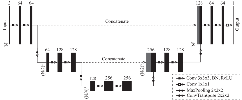
The CNN architecture used is inspired by the U-net architecture originally developed for image segmentation [33] (Fig. 1). However, the output activation function is replaced by a linear activation function for the regression task considered in this work. A similar architecture for the approximation of flame surface density has already been used successfully [22, 21]. Using $64$ channels in the first multi-channel feature map instead of $32$ in Refs [22, 21] increased the accuracy of the approximation of $\overline{\dot{\omega}}$ (Eq. (2.7)) in the present work. In total, the network comprises $5,424,193$ trainable parameters.

Figure 1: U-net type architecture used in the present work. Each black box corresponds to a multi-channel feature map. The number of channels is denoted on top of the box. The input sample has three channels: $\widetilde{c}$, $\widetilde{\phi}$ and $\delta_{L}^{0}/\delta_{L}^{1}$. The ratio $\delta_{L}^{0}/\delta_{L}^{1}$ is the inverse of the laminar flame thickening due to filtering (Section 2.3.2). The original size of the cubic sample is $\mathrm{N^{3}}$. It is then reduced to $\mathrm{(N/2)^{3}}$ and $\mathrm{(N/4)^{3}}$ during the contracting path before to go back to the original size during the expansive path. Gray boxes represent copied feature maps. The arrows denote the different operations

2.3 Data generation and training strategy

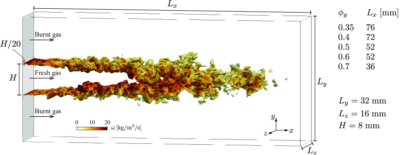
The data generation strategy consists in filtering and downsampling data from DNS to emulate LES data with known filtered quantities. The configuration chosen to generate training data is a slot burner (Fig. 2) at constant pressure $P=1$ atm and fresh gas temperature $T^{u}=300$ K, as in Refs [22, 21]. The physical domain consists of a central inlet where a premixed H₂-air mixture flows at a bulk velocity $U_{b}=24$ $\mathrm{m/s}$ with velocity fluctuation $u^{\prime}=2.4$ $\mathrm{m/s}$, surrounded by two laminar coflows where burnt gas flows at a bulk velocity $U_{c}=3.6$ $\mathrm{m/s}$. The injection of turbulence at the central inlet corresponds to homogeneous and isotropic turbulence using a Passot-Pouquet turbulence spectrum [26] with an integral length scale $l_{t}=2$ mm. The domain is rectangular with periodic boundary conditions in the $z$-direction. Adiabatic walls are specified in the $y$-direction. Both inlets and outlet are specified in the $x$-direction. Exact dimensions are annotated on Fig. 2. The configuration is very similar to that used in Refs [5, 10, 12] to study H₂-air and H₂/NH₃-air premixed turbulent flames. This configuration is computed for five different equivalence ratios (Table 1) to assess the ability of the CNN to approximate the reaction rate over a range of equivalence ratios. All other parameters are kept constant. The Reynolds number of the central inlet is about $10,000$ for all cases.

Figure 2: Diagram of the slot burner configuration used to generate the DNS database. The flame is depicted by an iso-surface at a progress variable $c=0.5$ colored by $\dot{\omega}=-\dot{\omega}_{\mathrm{H_{2}}}$. The dimensions of the domain are annotated on the right. The length $L_{x}$ is adapted to the length of the turbulent flame brush, which is function of the global equivalence ratio $\phi_{g}$

Table 1: Global equivalence ratio $\phi_{g}$ for the five different DNS cases. The laminar flame characteristic values are also indicated. $S_{L}^{0}$ is the laminar flame speed, $\delta_{th,L}^{0}$ the laminar thermal flame thickness, $T^{ad}$ the adiabatic flame temperature

Case	$\phi_{g}=0.35$	$\phi_{g}=0.4$	$\phi_{g}=0.5$	$\phi_{g}=0.6$	$\phi_{g}=0.7$
$S_{L}^{0}$ [m/s]	$9.453\cdot 10^{-2}$	$1.925\cdot 10^{-1}$	$4.972\cdot 10^{-1}$	$8.845\cdot 10^{-1}$	$1.302$
$\delta_{th,L}^{0}$ [m]	$1.146\cdot 10^{-3}$	$7.176\cdot 10^{-4}$	$4.809\cdot 10^{-4}$	$4.339\cdot 10^{-4}$	$4.171\cdot 10^{-4}$
$T^{ad}$ [K]	$1311$	$1428$	$1646$	$1844$	$2020$

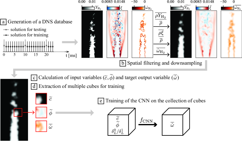
The data generation and training strategy is based on processing multiple snapshots from the five DNSs (Fig. 3):

1. The five DNS cases (Table 1) are computed for $59$ ms from a statistically steady state. Three-Dimensional (3D) instantaneous solutions are saved every ms. Solutions with an index multiple of 10 are set aside for testing after training. All other solutions are used for training and validation data. This generates 6 solutions for testing and 54 solutions for training and validation data for each DNS case.

2. A spatial filtering is performed on each solution to obtain $\overline{\rho}$, $\overline{\rho Y_{\mathrm{H_{2}}}}$, $\overline{\rho\xi}$ and $\overline{\dot{\omega}_{\mathrm{H_{2}}}}$. The filtered variables are downsampled to a coarser grid, representing an LES grid. The filtering and downsampling operation is described in Section 2.3.2.

3. From the filtered variables, $\widetilde{c}$, $\widetilde{\phi}$ and $\overline{\dot{\omega}}$ (Eqs (2.3), (2.6) and (2.4)) are calculated.

4. It is important that the CNN does not learn the specific configuration of the slot burner, but only learns generic flame elements. Therefore, training is not carried out on the entire domain, but rather on randomly selected cubes in the domain as in Refs [22, 21]. A number of cubes per solution $N_{c}=40$ is randomly extracted for training and validation. The size of the cubes is $16\times 16\times 16$ points.

5. The CNN is trained to approximate $\overline{\dot{\omega}}$ (Eq. (2.7)) using data from the cubic samples. 10% of samples are randomly selected and set aside for validation, the rest are used for training. The complete description of the training is given in Section 2.3.3.

Figure 3: Diagram of the strategy used to generate data and train the CNN. $\delta_{L}^{0}/\delta_{L}^{1}$ is the inverse of the laminar flame thickening due to filtering (Section 2.3.2). $\widetilde{\phi}$ is calculated from $\widetilde{\xi}$ using Eq. (2.6)

2.3.1 Direct numerical simulation

DNS of the slot burner cases (Table 1) are performed using the AVBP [35, 13] massively parallel code solving the compressible multi-species Navier-Stokes equations. A third order accurate Taylor–Galerkin scheme is adopted for discretization of the convective terms [9]. Navier-Stokes Characteristic Boundary Conditions [29] are imposed at the inlets and at the outlet. Viscosity follows a power law function of temperature. Thermal diffusivity is computed from the viscosity using a constant Prandtl number: $\mathrm{Pr}=0.66$. Species diffusion fluxes rely on Hirschfelder and Curtis approximation [16] where diffusion coefficients are computed using a constant Schmidt number specific for each species (Table 2). This approach takes into account non-unity Lewis number and differential diffusion between the different species. Hydrogen chemical kinetics relies on the San Diego mechanism [34], already successfully used for H₂-air premixed combustion in Ref. [10]. This mechanism comprises $9$ species and $21$ reactions.

Table 2: Schmidt $\mathrm{Sc}_{k}$ and Lewis $\mathrm{Le}_{k}$ numbers for the species used for the DNS of H₂-air flames

Species $k$	$\mathrm{H_{2}}$	$\mathrm{H}$	$\mathrm{O_{2}}$	$\mathrm{OH}$	$\mathrm{O}$	$\mathrm{H_{2}O}$	$\mathrm{HO_{2}}$	$\mathrm{H_{2}O_{2}}$	$\mathrm{N_{2}}$
$\mathrm{Sc}_{k}$	$0.23$	$0.14$	$0.80$	$0.53$	$0.52$	$0.58$	$0.80$	$0.81$	$0.91$
$\mathrm{Le}_{k}$	$0.34$	$0.21$	$1.20$	$0.80$	$0.79$	$0.88$	$1.21$	$1.22$	$1.37$

The mesh is a homogeneous cartesian grid with constant element size $\Delta_{x}=0.1$ mm. This gives a resolution index $\mathrm{RI}=\delta_{th,L}^{0}/\Delta_{x}+1$ that varies between $12.5$ and $5.2$ for $\phi_{g}$ between $0.35$ and $0.7$. The length of the domain in the $x$-direction $L_{x}$ is adapted to the length of turbulent the flame brush. It varies from $76$ mm for $\phi_{g}=0.35$ to $36$ mm for $\phi_{g}=0.7$ (Fig. 2). The number of grid points accordingly varies from $39$ to $19$ million. Calculations were carried out on the new Alps Research Infrastructure at the Swiss National Supercomputing Centre (CSCS) using AMD EPYC 7742 CPUs. A total of $1.6$ million core-hours were used to generate the database. Depending on the grid size, computations are performed using between $5,120$ and $2,560$ computing cores with good efficiency thanks to the massively parallel computing ability of the AVBP code.

2.3.2 Filtering and downsampling

A spatial filtering is performed to obtain $\overline{\rho}$, $\overline{\rho Y_{\mathrm{H_{2}}}}$, $\overline{\rho\xi}$ and $\overline{\dot{\omega}_{\mathrm{H_{2}}}}$, in order to calculate $\widetilde{c}$, $\widetilde{\phi}$ and $\overline{\dot{\omega}}$ (Eqs (2.3), (2.6) and (2.4)). The filtered quantity of a variable $Q$ from the DNS field is defined as

$$\overline{Q}(\mathbf{x})=\int Q\left(\mathbf{x}^{\prime}\right)F\left(\mathbf{x}-\mathbf{x}^{\prime}\right)d\mathbf{x}^{\prime}\,\text{,}$$ (2.8)

where $F$ is the spatial filter. The filtered 3D fields are obtained by successively filtering on each direction $x$, $y$ and $z$ using a One-Dimensional (1D) Gaussian filter. The 1D filter function is written in discrete form as

$$F(u)=\begin{cases}e^{-\frac{1}{2}\left(\frac{u}{\sigma}\right)^{2}}&\text{ if }u\in\left[-z\;..+z\right]\\ 0&\text{ otherwise }\end{cases}\,\text{with}\,z=4\sigma\,\text{,}$$ (2.9)

and then normalized by its sum $\sum_{u=-z}^{z}F(u)$. The filtered fields are then downsampled to a coarser grid to emulate LES fields. Three different standard deviations $\sigma$ are used in this work to emulate three different LES resolutions (Table 3). For each $\sigma$, a downsampling factor DSF is associated. It is chosen so as to have a LES grid with a resolution index $\mathrm{RI}=\delta_{c,L}^{1}/\Delta_{x}+1$ of about 6. $\delta_{c,L}^{0}$ and $\delta_{c,L}^{1}$ are the laminar flame thickness based on the progress variable of a non-filtered and filtered 1D flame

$$\delta_{c,L}^{0}=\left(\mathrm{max}\left|\nabla c\right|\right)^{-1}\,\text{and}\,\delta_{c,L}^{1}=\left(\mathrm{max}\left|\nabla\widetilde{c}\right|\right)^{-1}\,\text{.}$$ (2.10)

Table 3: Flame characteristics for the three sets of LES parameters ($\sigma$, DSF) used in this work. $\Delta_{x}$ is the grid cell size, equals to DSF times the original cell size of $0.1$ mm. $\delta_{c,L}^{0}$ and $\delta_{c,L}^{1}$ are the laminar flame thickness based on the progress variable of a non-filtered and filtered 1D flame (Eq. (2.10)). $\mathrm{RI}=\delta_{c,L}^{1}/\Delta_{x}+1$ is the resolution index of the filtered flame on the LES grid

	Case	$\phi_{g}=0.35$	$\phi_{g}=0.4$	$\phi_{g}=0.5$	$\phi_{g}=0.6$	$\phi_{g}=0.7$
$\sigma=4$ $\mathrm{DSF}=2$ $\Delta_{x}=0.2$ mm	$\delta_{c,L}^{1}$ [m]	$1.41\cdot 10^{-3}$	$1.06\cdot 10^{-3}$	$9.28\cdot 10^{-4}$	$9.01\cdot 10^{-4}$	$9.09\cdot 10^{-4}$
	$\delta_{c,L}^{0}/\delta_{c,L}^{1}$	$0.81$	$0.59$	$0.41$	$0.36$	$0.33$
	RI	$8.03$	$6.30$	$5.64$	$5.51$	$5.55$
$\sigma=8$ $\mathrm{DSF}=4$ $\Delta_{x}=0.4$ mm	$\delta_{c,L}^{1}$ [m]	$2.06\cdot 10^{-3}$	$1.83\cdot 10^{-3}$	$1.75\cdot 10^{-3}$	$1.75\cdot 10^{-3}$	$1.75\cdot 10^{-3}$
	$\delta_{c,L}^{0}/\delta_{c,L}^{1}$	0.55	0.34	0.21	0.18	0.17
	RI	$6.16$	$5.58$	$5.38$	$5.36$	$5.37$
$\sigma=16$ $\mathrm{DSF}=8$ $\Delta_{x}=0.8$ mm	$\delta_{c,L}^{1}$ [m]	$3.66\cdot 10^{-3}$	$3.53\cdot 10^{-3}$	$3.47\cdot 10^{-3}$	$3.45\cdot 10^{-3}$	$3.45\cdot 10^{-3}$
	$\delta_{c,L}^{0}/\delta_{c,L}^{1}$	$0.31$	$0.18$	$0.11$	$0.09$	$0.09$
	RI	$5.58$	$5.41$	$5.34$	$5.32$	$5.31$

2.3.3 Training method

The generated cubic samples (Fig. 3) of size $16\times 16\times 16$ points are used to train the CNN to approximate $\overline{\dot{\omega}}$ (Eq. (2.7)). A set of 10% of the samples is randomly selected to form a validation dataset and monitor overfitting. The remaining samples are used for training. At each epoch, each cubic sample in the training dataset has a $25$% probability of undergoing between one and three $90^{\circ}$ rotations along any axis, or of being flipped in any direction. It is done to add variability to the orientation of the flame front in the dataset. The model must have no preferential orientation and learn an isotropic function.

Training is accomplished by backpropagation. The trainable parameters of the CNN are updated iteratively on batches of data from the training dataset by stochastic gradient descent with the AdamW optimizer [17, 23]. The parameters are adjusted to minimize the Mean Squared Error (MSE) loss function over all output pixels of the prediction compared to the target. The batch size per GPU is $200$ and the training is terminated after $1,500$ epochs. The base learning rate equals $10^{-3}$. The evolution of the loss function on the training and validation datasets during training is given in Section 3.

The PyTorch [2] Python library is used to implement and train the CNN. The Distributed Data Parallel (DDP) feature in PyTorch is employed to parallelize the training process across four NVIDIA H100 GPUs. Each GPU performs its own forward and backward pass on a subset of the training dataset. The gradients computed on each GPU are then synchronized and averaged to update the model parameters. Training performances are reported in Section 3.

3 Results and discussion

3.1 Training and testing

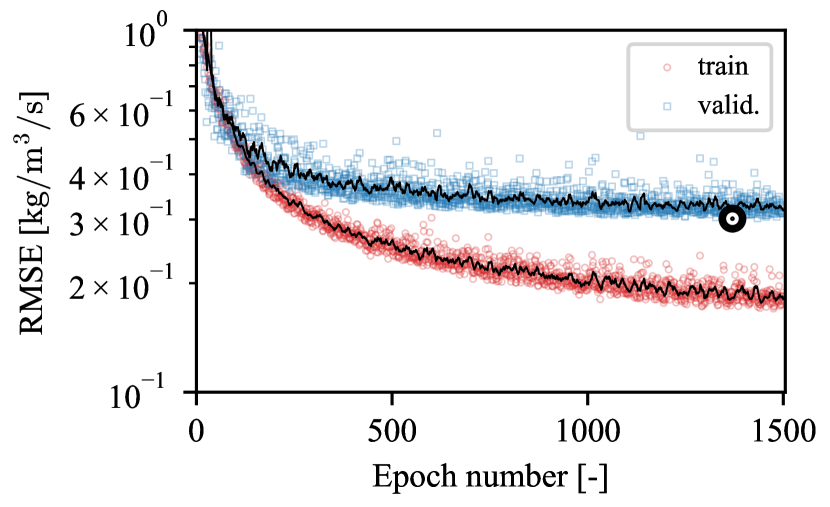
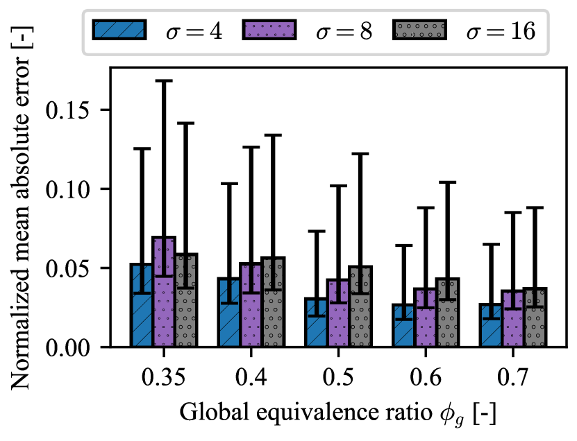
The training and validation database comprises $40\times 54\times 5\times 3=32,400$ cubic samples ($40$ random cubes per solution, $54$ solutions per case, $5$ different equivalence ratios, $3$ different sets of LES parameters (filtering and downsampling)). $3,240$ ($10$%) of these cubes are randomly set aside for validation. Training the CNN model for $1,500$ epochs on this database takes $47$ minutes. $1,500$ epochs are sufficient because the loss function evaluated on the validation dataset no longer decreases significantly (Fig. 4). The set of model parameters giving rise to the lowest loss is selected as the best model (black circle in Fig. 4). This best model is used to assess the ability of the CNN to approximate burning rates on the test solutions (full domain, never seen during training). The Normalized Mean Absolute Error (NMAE) is used to estimate the accuracy of the CNN model (Fig. 4). It is defined as:

$$\mathrm{NMAE}=\frac{1}{\mathrm{mean}\left(\overline{\dot{\omega}}^{\ast}\right)}\frac{1}{N}\sum_{i=1}^{N}\left|\overline{\dot{\omega}}^{\ast}_{i}-\overline{\dot{\omega}}^{\mathrm{NN}}_{i}\right|\,\text{,}$$ (3.1)

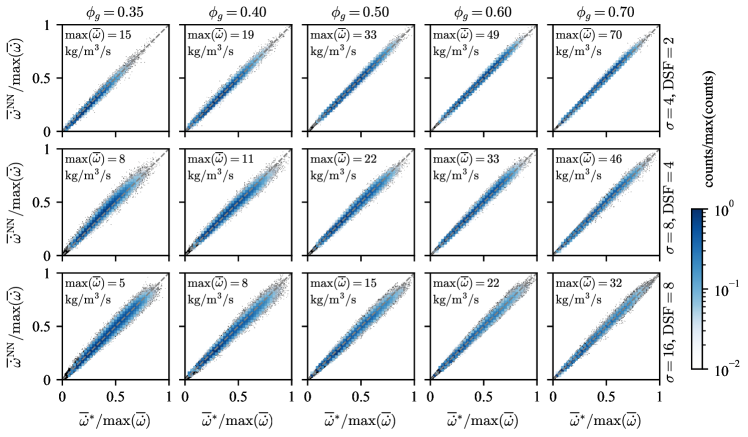
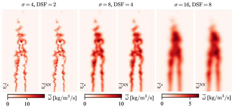
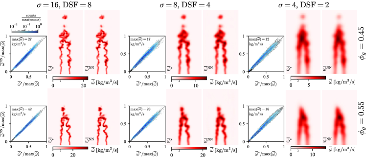
where $\overline{\dot{\omega}}^{\ast}$ is the filtered burning rate from the DNS dataset and $\overline{\dot{\omega}}^{\mathrm{NN}}$ is the filtered burning rate modeled by the CNN. The mean absolute error is only about $5$% of the average burning rate for all cases. The very high accuracy of the CNN model is confirmed by the distribution of CNN-modeled burning rate $\overline{\dot{\omega}}^{\mathrm{NN}}$ versus ground-truth filtered burning rate $\overline{\dot{\omega}}^{\ast}$ (Fig. 5). The log-normalized Two-Dimensional (2D) histograms show a large majority of points on the $x=y$ axis (i.e. perfect agreement). Figure 5 shows a visualization of the result using a planar cut through a test solution for the case $\phi_{g}=0.4$ and for the three sets of LES parameters $\left(\sigma,\mathrm{DSF}\right)$. One can see the ability of the CNN to retrieve the extremely complex turbulent flame topology for all filter sizes. Even the burning pockets detached from the main flame brush are correctly modeled by the CNN. This is true for all other equivalence ratios. The visualization of the cases $\phi_{g}=0.35$, $0.5$, $0.6$ and $0.7$ are given as supplementary material to avoid overloading the manuscript.

Figure 4: Left: Evolution of the Root Mean Square Error (RMSE) during training, evaluated over the training dataset (red circles) and the validation dataset (blue squares). Black solid lines are moving averages of the RMSE. The black circle shows the lowest RMSE over the validation dataset. The model parameters at this specific epoch are selected. Right: Normalized mean absolute error over the testing solutions (Eq. (3.1)) for the different equivalence ratios and LES parameters used for building the training dataset. Error bars show first and third quartiles of the data points

Figure 5: Scatter plots with 2D histograms: CNN-modeled burning rate $\overline{\dot{\omega}}^{\mathrm{NN}}$ versus ground-truth filtered burning rate $\overline{\dot{\omega}}^{\ast}$. Individual values are normalized by the maximum burning rate in the datasets. The points used for the histograms have a progress variable $c$: $0.05\leq c\leq 0.95$. Histogram values below the colour scale are transparent. Gray dashed line indicates $x=y$ (i.e. zero error). Each column corresponds to a global equivalence ratio. Each row corresponds to a set of LES parameters (filtering and downsampling). Data are collected from the testing solutions

Figure 6: Planar cut normal to the $z$-axis, in the middle of the domain, colored by the ground-truth filtered burning rate $\overline{\dot{\omega}}^{\ast}$ and the CNN-modeled burning rate $\overline{\dot{\omega}}^{\mathrm{NN}}$ for three sets of LES parameters. The global equivalence ratio is $\phi_{g}=0.4$. The complex turbulent flame topology of the burning rates is remarkably well reproduced by the CNN

3.2 Generalization ability

The ability of the CNN model to generalize outside the cases for which it has been trained is now assessed. For this, two new sets of LES parameters $\left(\sigma=6,\mathrm{DSF}=3\right)$ and $\left(\sigma=12,\mathrm{DSF}=6\right)$, and two new equivalence ratios $\phi_{g}=0.45$ and $0.55$ are used.

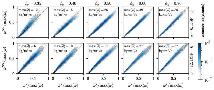
Filtering and downsampling with the two new sets of LES parameters are performed on test solutions of the existing DNS with global equivalence ratios $\phi_{g}=0.35$, $0.4$, $0.5$, $0.6$ and $0.7$. Although the distribution of points $\overline{\dot{\omega}}^{\mathrm{NN}}$ versus $\overline{\dot{\omega}}^{\ast}$ is a little more scattered (Fig. 7), the majority of the CNN-modeled burning rates are in very good agreement with their ground-truth counterparts. This demonstrates the ability of the model to generalize between two LES filter sizes for which it has been trained. It is important to note, however, that training with all three filter sizes (Tab. 3) is necessary to achieve this result. We have tried to train the CNN with only two filter sizes: $\sigma=4$ and $16$, and found that the resulting model has a significant bias for $\sigma=8$, see supplementary material.

The ability of the model to approximate burning rates for other global equivalence ratios is now assessed. For this, two new DNS are performed with a global equivalence ratio $\phi_{g}=0.45$ and $0.55$ and six solutions per DNS (snapshot every $1$ ms) are used to evaluate the model on the filter sizes $\sigma=4$, $8$ and $16$ (Fig. 8). The distribution of points $\overline{\dot{\omega}}^{\mathrm{NN}}$ versus $\overline{\dot{\omega}}^{\ast}$ is a little more scattered compared to inference on solutions with a global equivalence ratios used for training. The majority of the points are nevertheless clustered along the $x=y$ axis: the approximation of the burning rates is still very good. The planar cuts show a flame topology very well retrieved by the CNN model. These excellent results are due to the large number of equivalence ratios included in the training dataset. We have trained the CNN with only $\phi_{g}=0.35$, $0.4$, $0.6$ and $0.7$ (i.e. without $\phi_{g}=0.5$) and that model is flawed for the global equivalence ratio $\phi_{g}=0.5$, see supplementary material.

These generalization results are very promising and show that a CNN model can generalize with a reasonable amount of training cases. This is particularly important with regard to the global equivalence ratio $\phi_{g}$. Computing a DNS for each global equivalence ratio has a significant computing cost. In contrast, the computational cost of a filtering and downsampling operation to produce a new set of LES parameters $\left(\sigma,\mathrm{DSF}\right)$ is negligible.

Figure 7: Scatter plots with 2D histograms: CNN-modeled burning rate $\overline{\dot{\omega}}^{\mathrm{NN}}$ versus ground-truth filtered burning rate $\overline{\dot{\omega}}^{\ast}$. Individual values are normalized by the maximum burning rate in the datasets. The points used for the histograms have a progress variable $c$: $0.05\leq c\leq 0.95$. Histogram values below the colour scale are transparent. Gray dashed line indicates $x=y$ (i.e. zero error). Each column corresponds to a global equivalence ratio. Each row corresponds to a set of LES parameters (filtering and downsampling). Data are collected from solutions with two sets of LES parameters that were not included into the training dataset. The CNN approximates the burning rates with good accuracy, demonstrating the ability to generalise to other LES parameters from which it has been trained

Figure 8: Scatter plots and 2D histograms together with planar cuts comparing CNN-modeled burning rate $\overline{\dot{\omega}}^{\mathrm{NN}}$ to ground-truth filtered burning rate $\overline{\dot{\omega}}^{\ast}$. See caption of Fig. 5 for a full description of how the histograms are constructed. The two global equivalence ratios $\phi_{g}=0.45$ and $0.55$ were not included in the training dataset. The CNN approximates the burning rates with high accuracy, demonstrating the ability to generalise to other equivalence ratios from which it has been trained

3.3 Comparison with a filtered tabulated chemistry approach

A filtered tabulated chemistry modeling is implemented to compare CNN results with an established approach for modeling filtered burning rates. In the filtered tabulated chemistry framework, the flame structure in the direction normal to the flame front is assumed identical to the structure of a planar 1D freely propagating premixed laminar flame [11]. For a given filter size, it is then possible to apply the filter operation introduced in Section 2.3.2 (Eqs (2.8) and (2.9)) to a precomputed 1D flame and extract the burning rates directly as

$$\overline{\dot{\omega}}=\overline{\dot{\omega}}^{\,+}\left(\widetilde{c}\right)\,\text{,}$$ (3.2)

where $\overline{\dot{\omega}}^{\,+}$ is the filtered burning rate of the 1D flame, mapped as a function of the filtered progress variable $\widetilde{c}$ for a given filter size $\sigma$. Flame wrinkling at the subfilter-scale level is lost in LES. A subfilter-scale wrinkling factor $\Xi$ needs to be applied to compensate for the loss in flame surface [30]. The filtered burning rate for filtered tabulated chemistry modeling therefore reads

$$\overline{\dot{\omega}}^{FC}=\Xi\,\overline{\dot{\omega}}^{\,+}\left(\widetilde{c}\right)\,\text{.}$$ (3.3)

The wrinkling factor $\Xi$ is usually modeled by algebraic expressions. Models based on a fractal description of the flame front [14, 15] are very common. They assume that in a range of physical scales bounded by an inner cutoff $\eta$ and an outer cutoff $L$, the flame front is a fractal surface of dimension $2\leq D_{f}\leq 3$. The wrinkling factor is given by

$$\Xi=\left(\frac{L}{\eta}\right)^{D_{f}-2}\,\text{.}$$ (3.4)

$L$ corresponds to the size of the largest unresolved wrinkles, which is of the order of the thickness of the LES flame estimated as $\delta_{c,L}^{1}$ (Eq. (2.10)). $\eta$ is the size of the smallest wrinkles and varies from $\eta=L$ (i.e. no unresolved wrinkling, $\Xi=1$) to $\eta=\delta_{c,L}^{0}$ (i.e. filling of the space by a flame surface of fractal dimension $D_{f}$ between cut-off scales $\delta_{c,L}^{0}$ and $L$, $\Xi=\left(L/\delta_{c,L}^{0}\right)^{D_{f}-2}$). The latter situation is reached when turbulence intensity is sufficiently high, which is often the case in practice [40, 39]. We then assume $\eta=\delta_{c,L}^{0}$ in Eq. (3.4), maximizing the flame surface density at the subfilter-scale level. The fractal dimension is estimated as $D_{f}=2.5$ following the work of Charlette et al. [8].

CNN-based modeling significantly outperforms the filtered tabulated chemistry one, especially for the lean cases (e.g. $\phi_{g}=0.35$ in Fig. 9). Due to the extremely high thermodiffusive effects in the very lean cases, the burning rates of the turbulent 3D field can be much higher than those in a freely propagating planar flame at the same global equivalence ratio $\phi_{g}$. For example, for the case $\phi_{g}=0.35$, $\sigma=4$, $\mathrm{DSF}=2$, the maximum burning rate in the 3D field $\mathrm{max}(\overline{\dot{\omega}}^{\ast})$ is about $17$ times greater than that in a laminar planar flame $\mathrm{max}(\overline{\dot{\omega}}^{\,+})$. This is due to local stretching and enrichment effects that are not taken into account by the tabulated chemistry approach we have implemented. The wrinkling factor $\Xi$ only accounts for flame surface density, and new models need to be developed. This $\phi_{g}=0.35$ case is a truly extreme test case to illustrate the strength of the CNN model. Tabulated chemistry modeling does not fail so spectacularly for equivalence ratios close to stoichiometry, where preferential and differential diffusion effects are less pronounced (e.g. $\phi_{g}=0.7$ in Fig. 9). The CNN results are still much more accurate thanks to the consideration of the 3D flame structure via successive convolutions.

Figure 9: Scatter plots of the CNN-modeled burning rate $\overline{\dot{\omega}}^{\mathrm{NN}}$ and the filtered tabulated chemistry burning rate $\overline{\dot{\omega}}^{\mathrm{FC}}$ (Eq. (3.3)) versus ground-truth filtered burning rate $\overline{\dot{\omega}}^{\ast}$. Individual values are normalized by the maximum burning rate in the datasets. Gray dashed line indicates $x=y$ (i.e. zero error). Two cases of LES parameter sets are presented for two global equivalence ratios: the lowest equivalence ratio $\phi_{g}=0.35$ for which the filtered tabulated chemistry is significantly flawed due to very strong thermodiffusive effects; the highest equivalence ratio $\phi_{g}=0.7$ for which thermodiffusive effects are less important

4 Conclusion and future work

Trustworthy LES of lean premixed hydrogen combustion requires advanced modeling methods considering thermodiffusive effects on burning rates at the subfilter-scale level. These effects are extremely complex and their coupling with turbulence is controversial, making the derivation of analytical models very difficult. We therefore propose a pure ML approach where a CNN is trained to approximate LES burning rates from emulated LES fields, generated by explicitly filtering many DNS snapshots. The configuration used to generate the training data is a slot burner where a turbulent flow of premixed H₂-air mixture is placed in between two coflows of burnt gas burnt at the same equivalence ratio. The training dataset is built up by performing five DNSs of this configuration, each with a unique global equivalence ratio. The DNS solutions are then filtered and downsampled using three different sizes to emulate LES solutions. Many small cubes are extracted from the solutions to train the CNN model so that it does not learn the specific configuration but rather generic flame elements, improving its generalization ability later on.

The trained CNN model retrieves burning rates with very high accuracy on the 3D full-scale test solutions. It is able to model burning rates in a very complex turbulent flame topology with flame elements detached from the main flame brush. In addition, the CNN approximates burning rates with low errors for filter and downsampling parameters and global equivalence ratios other than those for which it has been trained. The ML-based modeling outperforms a priori a classical filtered tabulated chemistry approach with correction for flame surface density due to subfilter-scale flame wrinkling. This is particularly true for very lean flames, where preferential diffusion effects are major and undermine modeling based on flame surface density.

These results are extremely promising. They demonstrate that it is possible to build an ML-based model of the burning rates of turbulent lean premixed H₂-air flames—an extremely challenging task—that can generalise outside the scope for which it has been trained. Generalisation is very important if we are really going to consider implementing this type of model in engineering simulation software. This work paves the way for a new modeling approach to turbulent H₂ combustion, which we want to pursue with the scientific community in the very near future.

We can then draw up a roadmap for integration into an LES code. First, the modeling of the diffusive fluxes remains to be addressed. It is usually done through simple gradient assumptions [30]. However, since diffusion plays an important role in the propagation speed of premixed flames [41, 18], a simple closure of this type may not be sufficient. If this is the case, we could consider training the CNN to approximate the diffusive fluxes using several output channels. Another option could be to derive analytical laws to correct the diffusive fluxes so as to retrieve appropriate flame propagation speeds. Second, there are a number of practical integration challenges to be tackled. In a massively parallel HPC code, the fluid domain is decomposed in many partitions distributed over the MPI tasks (typically one MPI per GPU). When inference is performed on each MPI, artefacts may appear at the boundaries of the partitions [37]. To avoid this, the inference must be given its neighboring context to produce overlapping predictions. However, this incurs additional MPI communication costs that must be evaluated on a case by case basis. Another major challenge is related to the voxel grid requirement for the CNN. If the CFD code uses an irregular grid that does not match the voxel/pixel structure, two grids have to be used: one for the fluid solver, one for the CNN inference. This requires the development of efficient methods for interpolating on-the-fly and transferring data between the two grids. The PhyDLL [37] open-source library is one effort that could help to address these issues. These questions will be the focus of a future project, now that we have shown that CNN-based modeling of the burning rates is possible with this work.

Acknowledgments

The authors gratefully acknowledge CERFACS for providing the LES solver AVBP and the antares and ARCANE libraries.

Funding Statement

This research was funded in part by the Swiss National Science Foundation (SNSF) under grant agreement No. 219938. This work was supported by a grant from the Swiss National Supercomputing Centre (CSCS) under project ID s1262.

Competing Interests

The authors declare none.

Data Availability Statement

The DNS database will be made available via BLASTNet https://blastnet.github.io/index.html.

Ethical Standards

The research meets all ethical guidelines, including adherence to the legal requirements of the study country.

Author Contributions

Q.M.: conceived the research project, performed the DNS, generated the database, trained the CNN, post-processed the results, performed the analysis, discussed the results, wrote the paper. C.J.L.: discussed the results, reviewed and edited the paper. N.N.: discussed the results, reviewed and edited the paper.

References

- Aniello et al., [2022] Aniello, A., Laera, D., Berger, L., Attili, A., and Poinsot, T. (2022). Introducing thermodiffusive effects in large-eddy simulation of turbulent combustion for lean hydrogen-air flames. Center for Turbulence Research, Proceedings of the Summer Program, pages 267–277.
- Ansel et al., [2024] Ansel, J., Yang, E., He, H., Gimelshein, N., Jain, A., Voznesensky, M., Bao, B., Bell, P., Berard, D., Burovski, E., Chauhan, G., Chourdia, A., Constable, W., Desmaison, A., DeVito, Z., Ellison, E., Feng, W., Gong, J., Gschwind, M., Hirsh, B., Huang, S., Kalambarkar, K., Kirsch, L., Lazos, M., Lezcano, M., Liang, Y., Liang, J., Lu, Y., Luk, C. K., Maher, B., Pan, Y., Puhrsch, C., Reso, M., Saroufim, M., Siraichi, M. Y., Suk, H., Zhang, S., Suo, M., Tillet, P., Zhao, X., Wang, E., Zhou, K., Zou, R., Wang, X., Mathews, A., Wen, W., Chanan, G., Wu, P., and Chintala, S. (2024). PyTorch 2: Faster Machine Learning Through Dynamic Python Bytecode Transformation and Graph Compilation. In Proceedings of the 29th ACM International Conference on Architectural Support for Programming Languages and Operating Systems, Volume 2, pages 929–947, La Jolla CA USA. ACM.
- [3] Berger, L., Attili, A., and Pitsch, H. (2022a). Intrinsic instabilities in premixed hydrogen flames: Parametric variation of pressure, equivalence ratio, and temperature. Part 1 - Dispersion relations in the linear regime. Combustion and Flame, 240:111935.
- [4] Berger, L., Attili, A., and Pitsch, H. (2022b). Intrinsic instabilities in premixed hydrogen flames: parametric variation of pressure, equivalence ratio, and temperature. Part 2 – Non-linear regime and flame speed enhancement. Combustion and Flame, 240:111936.
- [5] Berger, L., Attili, A., and Pitsch, H. (2022c). Synergistic interactions of thermodiffusive instabilities and turbulence in lean hydrogen flames. Combustion and Flame, 244:112254.
- Bilger et al., [1990] Bilger, R., Stårner, S., and Kee, R. (1990). On reduced mechanisms for methane-air combustion in nonpremixed flames. Combustion and Flame, 80(2):135–149.
- Boger et al., [1998] Boger, M., Veynante, D., Boughanem, H., and Trouvé, A. (1998). Direct numerical simulation analysis of flame surface density concept for large eddy simulation of turbulent premixed combustion. Symposium (International) on Combustion, 27(1):917–925.
- Charlette et al., [2002] Charlette, F., Meneveau, C., and Veynante, D. (2002). A power-law flame wrinkling model for LES of premixed turbulent combustion Part I: non-dynamic formulation and initial tests. Combustion and Flame, 131(1-2):159–180.
- Colin and Rudgyard, [2000] Colin, O. and Rudgyard, M. (2000). Development of High-Order Taylor–Galerkin Schemes for LES. Journal of Computational Physics, 162(2):338–371.
- Coulon et al., [2023] Coulon, V., Gaucherand, J., Xing, V., Laera, D., Lapeyre, C., and Poinsot, T. (2023). Direct numerical simulations of methane, ammonia-hydrogen and hydrogen turbulent premixed flames. Combustion and Flame, 256:112933.
- Fiorina et al., [2010] Fiorina, B., Vicquelin, R., Auzillon, P., Darabiha, N., Gicquel, O., and Veynante, D. (2010). A filtered tabulated chemistry model for LES of premixed combustion. Combustion and Flame, 157(3):465–475.
- Gaucherand et al., [2024] Gaucherand, J., Laera, D., Schulze-Netzer, C., and Poinsot, T. (2024). DNS of Turbulent Premixed Ammonia/Hydrogen Flames: The Impact of Thermo-Diffusive Effects. Flow, Turbulence and Combustion, 112(2):587–614.
- Gicquel et al., [2011] Gicquel, L. Y., Gourdain, N., Boussuge, J.-F., Deniau, H., Staffelbach, G., Wolf, P., and Poinsot, T. (2011). High performance parallel computing of flows in complex geometries. Comptes Rendus Mécanique, 339(2-3):104–124.
- Gouldin, [1987] Gouldin, F. (1987). An application of fractals to modeling premixed turbulent flames. Combustion and Flame, 68(3):249–266.
- Gouldin et al., [1989] Gouldin, F., Bray, K., and Chen, J.-Y. (1989). Chemical closure model for fractal flamelets. Combustion and Flame, 77(3-4):241–259.
- Hirschfelder et al., [2010] Hirschfelder, J. O., Curtiss, C. F., and Bird, R. B. (2010). Molecular theory of gases and liquids. Wiley, Hoboken, NJ.
- Kingma and Ba, [2017] Kingma, D. P. and Ba, J. (2017). Adam: A Method for Stochastic Optimization. arXiv:1412.6980 [cs].
- Kuo, [2005] Kuo, K. K. (2005). Principles of combustion. John Wiley, Hoboken, NJ, 2nd ed edition.
- Lapenna et al., [2021] Lapenna, P. E., Berger, L., Attili, A., Lamioni, R., Fogla, N., Pitsch, H., and Creta, F. (2021). Data-driven subfilter modelling of thermo-diffusively unstable hydrogen–air premixed flames. Combustion Theory and Modelling, 25(6):1064–1085.
- Lapenna et al., [2024] Lapenna, P. E., Remiddi, A., Molinaro, D., Indelicato, G., and Creta, F. (2024). A-posteriori analysis of a data-driven filtered wrinkled flamelet model for thermodiffusively unstable premixed flames. Combustion and Flame, 259:113126.
- Lapeyre et al., [2018] Lapeyre, C. J., Misdariis, A., Cazard, N., and Poinsot, T. (2018). A-posteriori evaluation of a deep convolutional neural network approach to subgrid-scale flame surface estimation. Center for Turbulence Research, Proceedings of the Summer Program, pages 349–358.
- Lapeyre et al., [2019] Lapeyre, C. J., Misdariis, A., Cazard, N., Veynante, D., and Poinsot, T. (2019). Training convolutional neural networks to estimate turbulent sub-grid scale reaction rates. Combustion and Flame, 203:255–264.
- Loshchilov and Hutter, [2019] Loshchilov, I. and Hutter, F. (2019). Decoupled Weight Decay Regularization. arXiv:1711.05101 [cs, math].
- Marble and Broadwell, [1997] Marble, F. E. and Broadwell, J. E. (1997). The coherent flame model for turbulent chemical reactions. Technical Report TRW-9-PU.
- Nikolaou et al., [2019] Nikolaou, Z. M., Chrysostomou, C., Vervisch, L., and Cant, S. (2019). Progress Variable Variance and Filtered Rate Modelling Using Convolutional Neural Networks and Flamelet Methods. Flow, Turbulence and Combustion, 103(2):485–501.
- Passot and Pouquet, [1987] Passot, T. and Pouquet, A. (1987). Numerical simulation of compressible homogeneous flows in the turbulent regime. Journal of Fluid Mechanics, 181:441–466.
- Peters, [1988] Peters, N. (1988). Laminar flamelet concepts in turbulent combustion. Symposium (International) on Combustion, 21(1):1231–1250.
- Petrov and Ghoniem, [1994] Petrov, C. and Ghoniem, A. (1994). An unsteady strained flame model for turbulent combustion simulations. In 32nd Aerospace Sciences Meeting and Exhibit, Reno, NV, U.S.A. American Institute of Aeronautics and Astronautics.
- Poinsot and Lelef, [1992] Poinsot, T. and Lelef, S. (1992). Boundary conditions for direct simulations of compressible viscous flows. Journal of Computational Physics, 101(1):104–129.
- Poinsot and Veynante, [2011] Poinsot, T. and Veynante, D. (2011). Theoretical and numerical combustion. CNRS, Toulouse, 3. ed edition.
- Pope, [1988] Pope, S. (1988). The evolution of surfaces in turbulence. International Journal of Engineering Science, 26(5):445–469.
- Regele et al., [2013] Regele, J. D., Knudsen, E., Pitsch, H., and Blanquart, G. (2013). A two-equation model for non-unity Lewis number differential diffusion in lean premixed laminar flames. Combustion and Flame, 160(2):240–250.
- Ronneberger et al., [2015] Ronneberger, O., Fischer, P., and Brox, T. (2015). U-net: Convolutional networks for biomedical image segmentation. In Navab, N., Hornegger, J., Wells, W. M., and Frangi, A. F., editors, Medical Image Computing and Computer-Assisted Intervention – MICCAI 2015, pages 234–241, Cham. Springer International Publishing.
- Saxena and Williams, [2006] Saxena, P. and Williams, F. A. (2006). Testing a small detailed chemical-kinetic mechanism for the combustion of hydrogen and carbon monoxide. Combustion and Flame, 145(1-2):316–323.
- Schonfeld and Rudgyard, [1999] Schonfeld, T. and Rudgyard, M. (1999). Steady and Unsteady Flow Simulations Using the Hybrid Flow Solver AVBP. AIAA Journal, 37(11):1378–1385.
- Seltz et al., [2019] Seltz, A., Domingo, P., Vervisch, L., and Nikolaou, Z. M. (2019). Direct mapping from LES resolved scales to filtered-flame generated manifolds using convolutional neural networks. Combustion and Flame, 210:71–82.
- Serhani et al., [2024] Serhani, A., Xing, V., Dupuy, D., Lapeyre, C., and Staffelbach, G. (2024). Graph and convolutional neural network coupling with a high-performance large-eddy simulation solver. Computers & Fluids, 278:106306.
- Trouvé and Poinsot, [1994] Trouvé, A. and Poinsot, T. (1994). The evolution equation for the flame surface density in turbulent premixed combustion. Journal of Fluid Mechanics, 278:1–31.
- Veynante and Moureau, [2015] Veynante, D. and Moureau, V. (2015). Analysis of dynamic models for large eddy simulations of turbulent premixed combustion. Combustion and Flame, 162(12):4622–4642.
- Veynante et al., [2012] Veynante, D., Schmitt, T., Boileau, M., and Moureau, V. (2012). Analysis of dynamic models for turbulent premixed combustion. Center for Turbulence Research, Proceedings of the Summer Program, pages 387–396.
- Williams, [2000] Williams, F. A. (2000). Combustion theory: the fundamental theory of chemically reacting flow systems. Combustion science and engineering series. CRC Press, 2. ed edition.