Experimental validation of a linear momentum and bluff-body model for high-blockage cross-flow turbine arrays

Abstract

The performance and near-wake characteristics of a turbine in a confined flow depend on the blockage ratio, defined as the ratio of the turbine projected area to the channel cross-sectional area. While blockage is understood to increase the power coefficient for turbine “fences” spanning a channel, most investigations at the upper range of practically-achievable blockage ratios have been theoretical or numerical in nature. Furthermore, while linear momentum actuator disk theory is frequently used to model turbines in confined flows, as confinement increases, the ability of this idealized model to describe performance and flow fields has not been established. In this work, the performance and near-wake flow field of a pair of cross-flow turbines are experimentally evaluated at blockage ratios from $30\%$ to $55\%$. The fluid velocity measured in the bypass region is found to be well-predicted by the open-channel linear momentum model developed by Houlsby et al. (2008), while the wake velocity is not. Additionally, self-similar power and thrust coefficients are identified across this range of blockage ratios when array performance is scaled by the modeled bypass velocity following Whelan et al.’s (2009) adaptation of the bluff-body theory of Maskell (1963). This result demonstrates that, despite multiple non-idealities, relatively simple models can quantitatively describe highly confined turbines. From this, an analytical method for predicting array performance as a function of blockage is presented. Overall, this work illustrates turbine performance at relatively high confinement and demonstrates the suitability of analytical models to predict and interpret their hydrodynamics.

1 Introduction

Flowing water in river and tidal channels is a promising source of renewable power. Individual turbines and arrays deployed in these channels can convert the energy in the fluid into mechanical power, and the efficiency of such turbines is influenced by how much of the channel cross-section they occupy. The characteristic scale of a row of turbines in a channel is represented by the blockage ratio, defined as the ratio between the turbine projected area and the channel cross-sectional area:

$$\beta=\frac{\mathrm{A_{turbines}}}{A_{\mathrm{channel}}}.$$ (1)

As the blockage ratio increases, the turbines present greater resistance to the oncoming flow. For a constant volumetric flow rate, this resistance, combined with confinement from the channel boundaries, increases flow through the turbine rotors relative to unconfined conditions. As a consequence, as confinement increases, so does turbine efficiency (Garrett & Cummins, 2007; Whelan et al., 2009; Nishino & Willden, 2012b; Vogel et al., 2016). While blockage augments the performance of all turbine designs, cross-flow turbines—which have an axis of rotation perpendicular to the direction of inflow—are particularly well-suited to exploit these physics since their rectangular projected area allows them to more easily achieve high blockage than circular axial-flow turbines.

Garrett & Cummins (2007) were the first to establish the theoretical basis for turbine performance in confined flows by applying one-dimensional linear momentum actuator disk theory (LMADT) to a turbine in a tidal channel. For relatively low Froude numbers, they showed that the maximum efficiency in confined flow was augmented by a factor of $(1-\beta)^{-2}$. Subsequent studies further generalized this analytical model. Houlsby et al. (2008) and Whelan et al. (2009) relaxed the assumption of low Froude number by allowing the free surface to deform in response to momentum extraction. Subsequently, Nishino & Willden (2012b, 2013) introduced a two-scale LMADT model for turbine arrays that considered confinement effects from both the channel boundaries (“global” blockage) and the presence of neighboring turbines within the array (“local” blockage). Vogel et al. (2016) later combined these approaches into a single model that incorporated both free surface deformation and inter-turbine proximity effects, and Dehtyriov et al. (2021) extended the two-scale model of Nishino & Willden (2012b) to an arbitrary number of scales (i.e., arrays of turbine sub-arrays) using a fractal-like approach.

A summary of prior experimental and numerical work evaluating turbine performance at multiple blockage ratios is provided in table 1. Across these studies, performance results are generally consistent and aligned with theory: for all types of turbines, as blockage increases, so do the thrust loading on the turbine, maximum efficiency, and optimal operating speed (i.e., tip-speed ratio or reduced frequency). Studies that examine the flow field near confined turbines (Battisti et al., 2011; Nishino & Willden, 2012a; McTavish et al., 2014; Dossena et al., 2015; Schluntz & Willden, 2015; Sarlak et al., 2016; Ross & Polagye, 2020b) find that an increase in blockage accelerates the flow through and around the turbine as predicted by theory, as well as narrows the turbine wake. Gauthier et al. (2016) and Kinsey & Dumas (2017) examined how blockage effects change with confinement asymmetry (i.e., different channel widths and heights at constant $\beta$) for various turbine types, and found turbine performance to be invariant to confinement asymmetry for width-to-height and height-to-width ratios approximately less than $3$. The interplay between rotor geometry and blockage effects has also been explored for cross-flow turbines by Goude & Ågren (2014) and for axial-flow turbines by Schluntz & Willden (2015) and Abutunis & Menta (2022). These studies found that higher-solidity rotors benefit more from blockage – a consequence of how their higher thrust coefficients couple with channel-level energetics.

Several of the studies in table 1 also explore analytical blockage corrections—which adjust observed turbine performance in confined flow to predict the performance of the same turbine in unconfined flow—and investigate their efficacy experimentally (Whelan et al., 2009; Battisti et al., 2011; Chen & Liou, 2011; Ross & Altman, 2011; Dossena et al., 2015; Jeong et al., 2018; Ross & Polagye, 2020a) or numerically (Gauthier et al., 2016; Kinsey & Dumas, 2017; Zilic de Arcos et al., 2020; Zhang et al., 2023). LMADT models are often the physical basis for blockage corrections (e.g., Barnsley & Wellicome, 1990; Whelan et al., 2009; Ross & Polagye, 2020a; Steiros et al., 2022; Dehtyriov et al., 2023). Such methods generally proceed from Glauert (1935) (originally introduced as a blockage correction for airplane propellers) by assuming that the thrust on a turbine depends on the incident freestream velocity, with LMADT employed to relate the confined and unconfined freestream velocities. In contrast, Whelan et al. (2009) found that an LMADT-based blockage correction inspired by the bluff-body theory of Maskell (1963) could be more effective for predicting the unconfined thrust coefficients of highly-loaded turbines. Unlike Glauert’s theory, a Maskell-inspired correction assumes that the thrust on a turbine depends on the velocity of the accelerated flow that bypasses it. However, none of these studies have demonstrated that the underlying LMADT models are actually descriptive of the flow field around confined turbines.

Experimental			Numerical
Author	Turbine Type	$\beta$ [%]	Author	Turbine Type	$\beta$ [%]
Takamatsu et al. (1985)	CFT	75, 95†	Nishino & Willden (2012a)	Actuator disk	3.1 - 50.3
Whelan et al. (2009)	AFT	5, 64	Consul et al. (2013)	CFT	12.5, 25, 50
McAdam et al. (2013a, b)	CFT	47, 59	Goude & Ågren (2014)	CFT	0, 12.5, 25, 50
Battisti et al. (2011)	CFT	2.8†, 10	Kolekar & Banerjee (2015)	AFT	4.2, 8.2, 11, 17, 20, 33, 42
Chen & Liou (2011)	AFT	10.2, 20.2, 28.3	Schluntz & Willden (2015)	AFT	0, 7.9, 19.6, 31.4
Ross & Altman (2011)	CFT (Savonius)	2, 3.5, 8	Gauthier et al. (2016)	Oscillating foil	0.2 - 60.5
Birjandi et al. (2013)	CFT	24.5 - 49.2†	Sarlak et al. (2016)	AFT	2, 5, 9, 20
McTavish et al. (2014)	AFT	6.3, 9.9, 14.3, 19.4, 25.4	Kinsey & Dumas (2017)	AFT	0, 10, 20, 50, 60
Gaurier et al. (2015)	AFT	1.2, 3.3, 4.8		CFT	0, 13, 26, 51
Ryi et al. (2015)	AFT	8.1, 18.0, 48.1	Badshah et al. (2019)	AFT	2 - 19
Dossena et al. (2015)	CFT	2.8†, 10	Gauvin-Tremblay & Dumas (2020)	CFT	5, 20, 40
Jeong et al. (2018)	CFT	3.5, 13.4, 24.7	Zilic de Arcos et al. (2020)	AFT	1, 5, 10, 20, 40
Ross & Polagye (2020a)	AFT	2, 35	Abutunis & Menta (2022)	AFT	4.2, 20.8, 41.6, 62.5
	CFT	3, 36	Zhang et al. (2023)	AFT	2, 2.8, 4.4, 7.9, 17.7
Ross & Polagye (2020b)	CFT	14, 36		CFT (Savonius)	2.5, 3.6, 5.6, 10, 22.5

• Value(s) estimated from provided turbine and channel dimensions.

Table 1: Summary of experimental and numerical studies that consider the effects of varying the blockage ratio for different types of turbines (axial-flow turbines are indicated by “AFT” and cross-flow turbines are indicated by “CFT”). Studies that consider $\beta\geq 30\%$ are bolded.

Although the studies in table 1 may appear to provide a comprehensive understanding of how confinement affects turbine performance, the upper end of blockage ratios that are achievable in a realistic channel ($\beta=30\%-60\%$) have been primarily explored through numerical simulation (e.g., Consul et al., 2013; Kinsey & Dumas, 2017; Abutunis & Menta, 2022). While the general trends in turbine performance and wake characteristics observed in simulation at these higher blockages are in agreement with theory, these have not been validated, in part due to a lack of equivalent experimental data. Only a handful of the experimental studies in table 1 consider blockage ratios greater than $30\%$, and of this subset, only Ross & Polagye (2020b) characterize the turbine wake. Furthermore, experimental studies that do explore the upper-end of blockage ratios consider only a sparse set of blockages (likely due to the difficulty in achieving a wide range of blockages while maintaining dynamic similarity (Hunt & Polagye, 2023)) which limits the ability to identify how performance trends evolve as a function of blockage. In addition, meaningful cross-comparisons between experiments are complicated by differences in rotor geometry, which can strongly influence performance (Schluntz & Willden, 2015; Hunt et al., 2024), and several studies convolve changes in blockage with changes in the Reynolds and Froude numbers (e.g., McAdam et al., 2013a, b; Birjandi et al., 2013). Given the lack of high-resolution experimental data at higher blockages, the computational methods used in numerical studies are often validated only at lower blockage (Consul et al., 2013; Kolekar & Banerjee, 2015; Gauthier et al., 2016; Kinsey & Dumas, 2017)—or not at all—before being used to draw conclusions at higher blockage. Consequently, although the general effects of blockage on turbine performance are well-known, there is residual uncertainty as to how these effects evolve at higher confinement. For these reasons, a high-resolution experimental examination of turbine performance and the associated near-wake flow field across the upper end of practically-achievable blockage ratios is warranted. In doing so, the accuracy of LMADT models for describing the near-wake flow field may also be evaluated, providing insight into the mechanics of blockage corrections.

Figure 1: Outline of the procedure in Sections 3 and 4 to interpret high blockage cross-flow turbine dynamics using experimental performance data, flow fields, and linear momentum theory. Key methodologies that are adapted from prior work are highlighted in gray boxes.

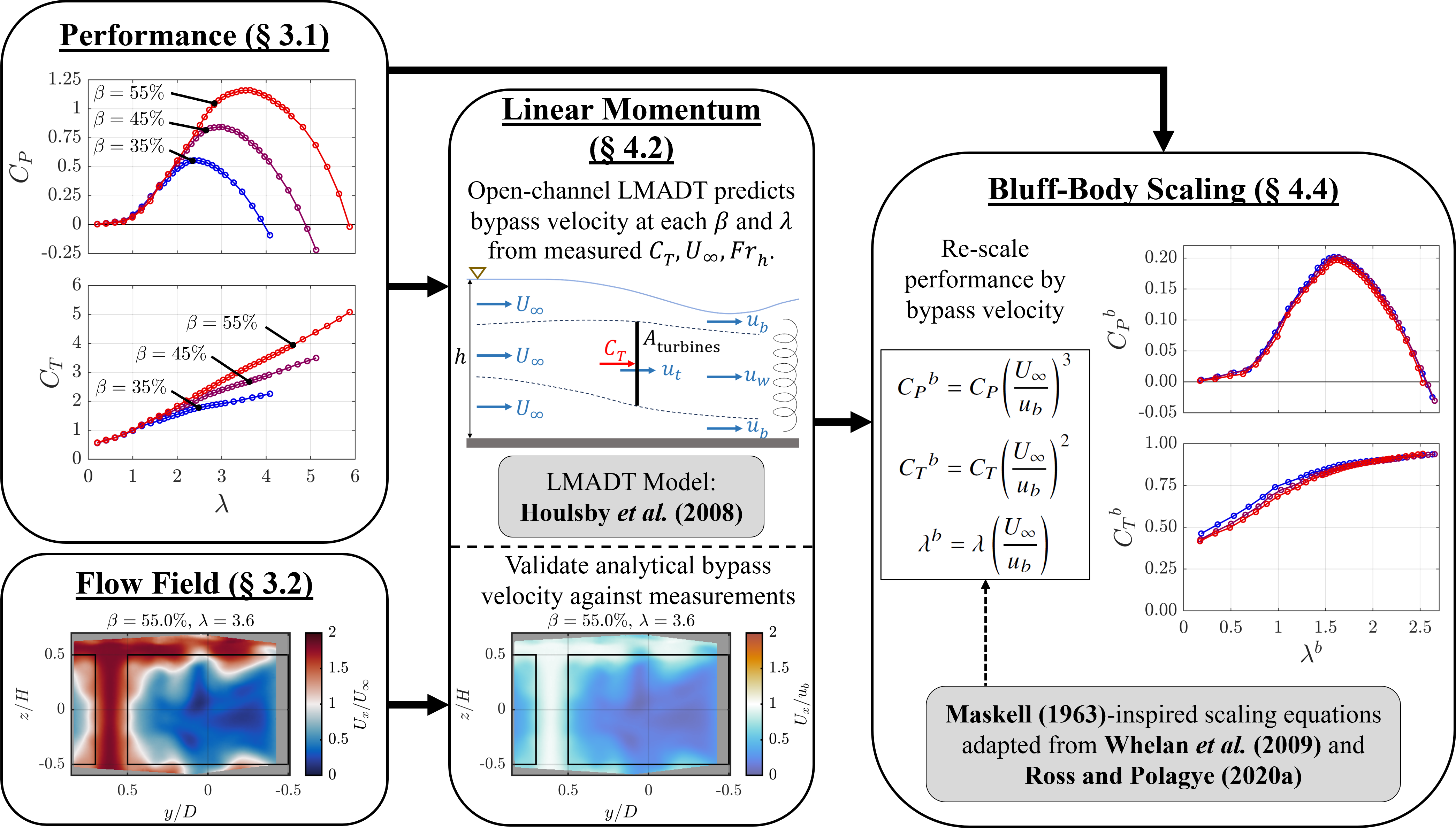
The objective of this work is to develop a more comprehensive understanding of performance and flow fields around a cross-flow turbine array at higher blockages. Such information can be used to understand the relevance of theory to non-ideal arrays that arguably violate multiple assumptions that underpin LMADT (e.g., treating the turbines as porous, non-rotating disks). Similarly, these experimental results provide a high-resolution data set for future validation of simulations at high confinement. To this end, a symmetric two-turbine array is tested in a recirculating water channel at blockage ratios ranging from $30\%$ to $55\%$, and particle image velocimetry (PIV) is used to measure the flow field in the near wake. In these experiments, the Reynolds and Froude numbers are controlled to avoid convolving changes in blockage with other relevant non-dimensional parameters (Ross & Polagye, 2022). Section 2 describes the experimental methods used to characterize array performance and flow fields, with trends in performance, near-wake velocities, and free surface deformation discussed in Section 3. In Section 4, the open-channel LMADT model developed by Houlsby et al. (2008) is applied to the experimental performance data to model the wake velocity, bypass velocity, and free surface deformation in the vicinity of the array. The analytically-modeled velocities are compared to measurements and are used to interpret high-blockage turbine hydrodynamics following Whelan et al.’s (2009) adaptation of the bluff-body theory of Maskell (1963). The procedure followed in Sections 3 and 4 is graphically outlined in figure 1 and methodologies that are adapted from prior work are highlighted. Based on the characteristic dynamics observed, a method for forecasting confined turbine performance based on linear momentum theory and Maskell’s (1963) bluff body theory (i.e., the reverse of the procedure in figure 1) is presented in Section 5.

2 Experimental Methods

2.1 Cross-Flow Turbine Test Setup

Experiments are conducted in the Alice C. Tyler recirculating water flume at the University of Washington. The flume has a test section that is 0.76 m wide and 4.88 m long, and can accommodate water depths up to 0.60 m and flow speeds up to ${\sim}\!1.1$ m/s. The flume is equipped with both a heater and chiller for temperature control, and can maintain water temperatures between $10$ ${}^{\circ}\mathrm{C}$ and $40$ ${}^{\circ}\mathrm{C}$.

The laboratory-scale array consists of two identical straight-bladed cross-flow turbines. The use of a pair of turbines, rather than an individual turbine, is motivated by the application of the research to understand the potential for confinement to reduce energy costs for turbine arrays. The rotors are two-bladed, consisting of a NACA 0018 profile with a 0.0742 m chord length ($c$) and mounted at a $-6^{\circ}$ (i.e., toe-out) preset pitch angle as referenced from the quarter chord. The blade span ($H$) is 0.215 m and the turbine diameter ($D$) is 0.315 m, measured at the outermost point swept by the blades. The blades are attached to the central driveshaft of each rotor using thin, hydrodynamic blade-end struts (NACA 0008 profile, 0.0742 m chord length). This arrangement results in an aspect ratio ($H/D$) of 0.68, chord-to-radius ratio ($c/R$) of 0.47, and solidity (product of the blade count and chord length relative to rotor circumference: $Nc/\pi D$, where $N$ is the blade count) of 0.15.

Figure 2: A rendering of the experimental test-rig, as viewed from upstream. The configuration shown corresponds to a blockage ratio of $40.1\%$.

Figure 3: Overhead view of the array layout in the Tyler flume, with key measured quantities annotated. The outermost circle swept by each turbine (with diameter $D$) is shown as a dashed blue circle.

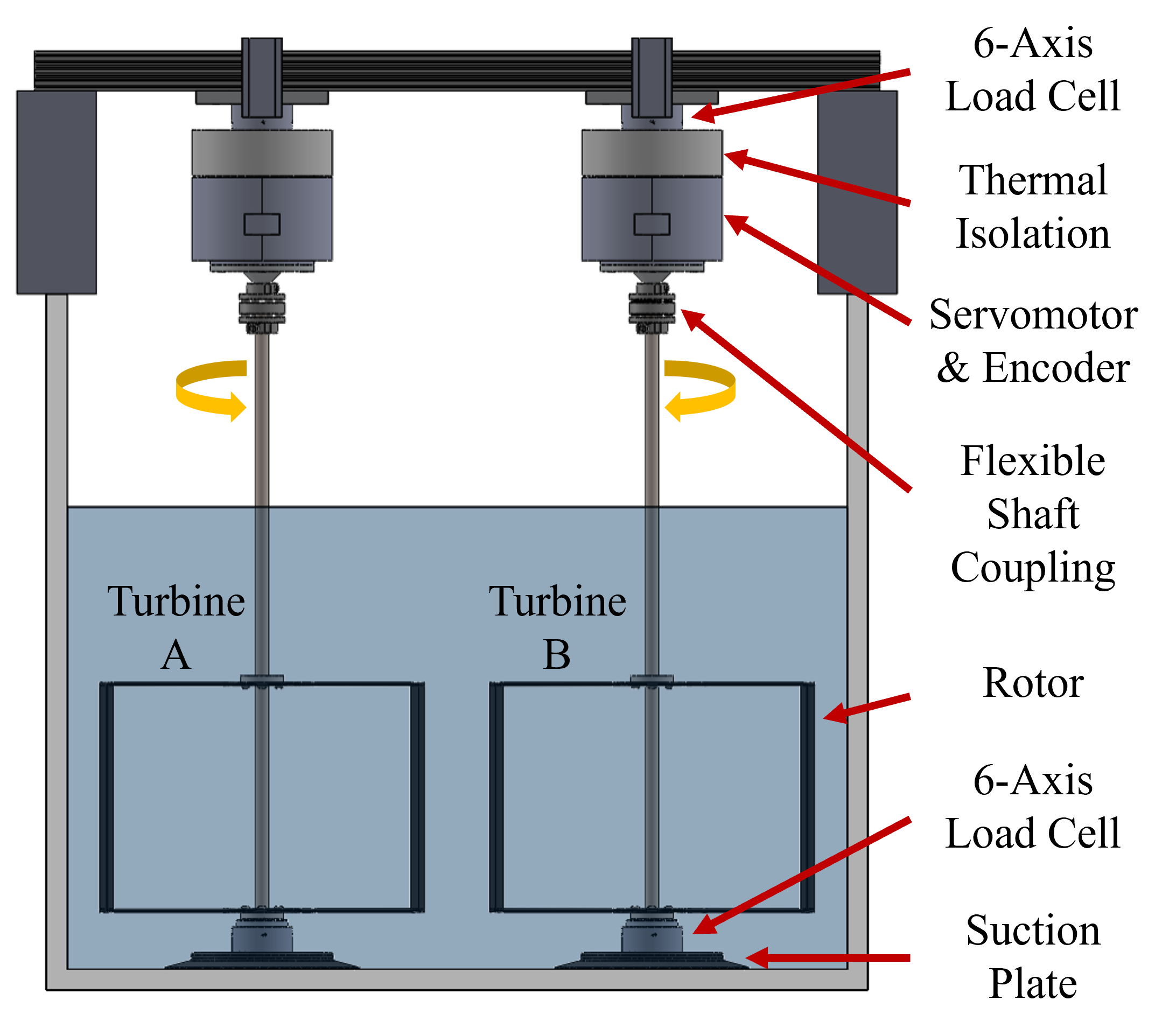
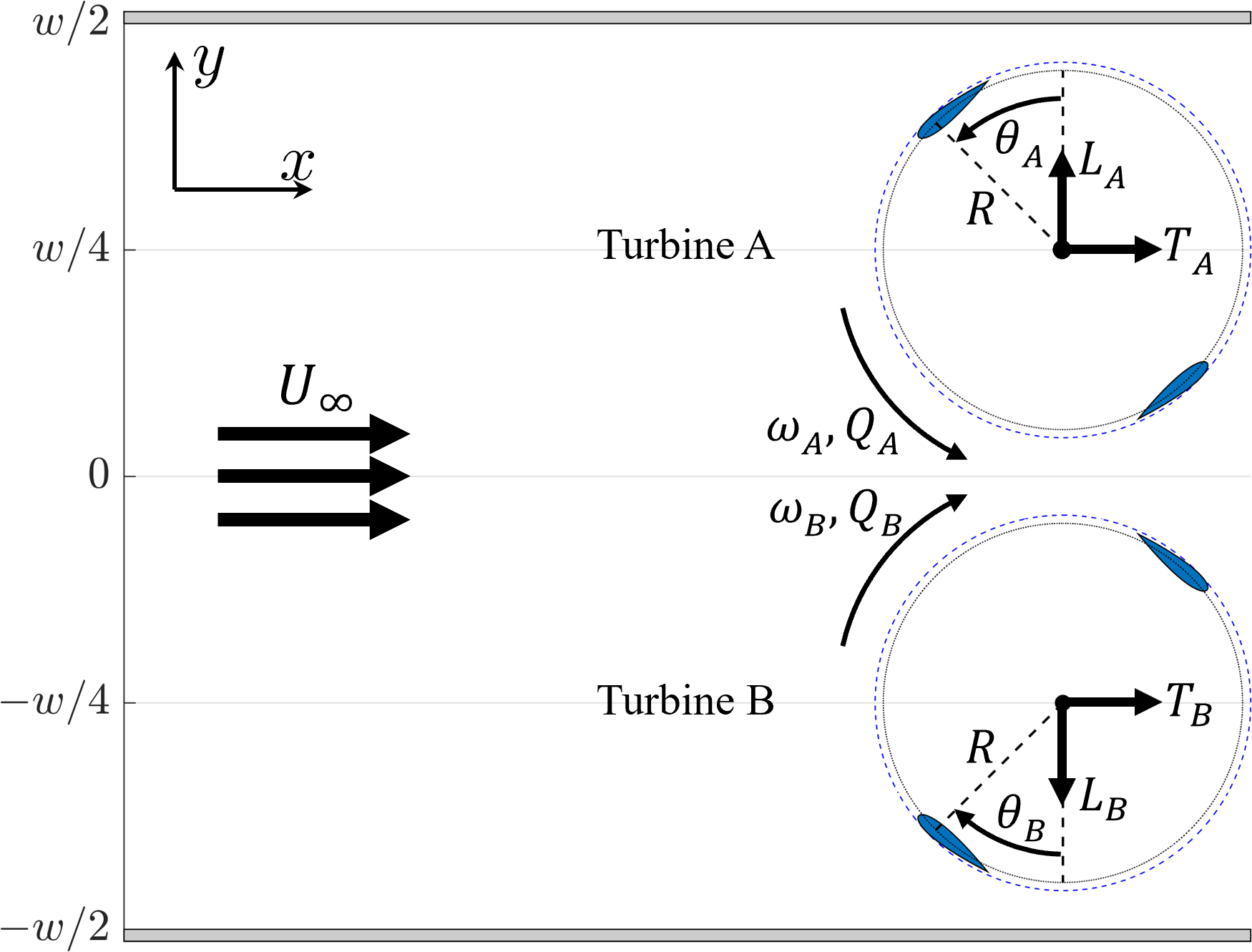
The two rotors, designated as “Turbine A” and “Turbine B”, are integrated into the experimental setup shown in figure 3, which consists of two identical test-rigs. The top of each turbine’s central shaft is connected by a flexible shaft coupling (Zero-Max SC040R) to a servomotor (Yaskawa SGMCS-05BC341) which regulates the rotation rate of the turbine. This control strategy yields similar time-average performance (Polagye et al., 2019) and wake characteristics (Araya & Dabiri, 2015) to applying a constant oppositional torque and reduces cycle-to-cycle variability . The angular position of each turbine is measured via the servomotor encoder ($2^{16}$ counts per revolution), from which the angular velocity is estimated. The bottom of each turbine’s central shaft sits in a bearing. The net forces and torques on each turbine are measured by a pair of 6-axis load cells: an upper load cell (ATI Mini45-IP65) connected to the servomotor through a thermal isolation assembly and fixed to a rigid crossbeam, and a lower load cell (ATI Mini45-IP68) mounted to the bottom bearing and fixed to the bottom of the flume via a suction plate. Measurements from the load cells and servomotor encoders for both turbines are acquired synchronously at 1000 Hz in MATLAB using two National Instruments PCIe-6353 DAQs.

The freestream velocity, $U_{\infty}$, is measured using an acoustic Doppler velocimeter (Nortek Vectrino Profiler) sampling at 16 Hz. The velocimeter sampled a single cell positioned laterally in the center of the flume, vertically at the array midplane, and $5D$ upstream of the turbines’ axes of rotation. Velocity measurements are despiked using the method of Goring & Nikora (2002). The water depth far upstream of the array ($5.8D$ upstream of the array centerline, centered laterally in the channel) as well as in the vicinity of the array ($0.5D$, $1.0D$, and $2.0D$ directly upstream and downstream of Turbine B) is measured using seven synchronized ultrasonic free surface transducers sampling at 0.5 Hz. As the array is symmetric about the channel centerline (figure 3) the streamwise free surface profile in the vicinity of Turbine B is assumed to be representative of that in the vicinity of Turbine A. The water temperature is measured using a temperature probe (Omega Ultra-Precise RTD) and maintained within $\pm 0.1^{\circ}\mathrm{C}$ of the target value during each experiment.

2.2 Non-Dimensional Parameters

For the two-turbine array, the blockage ratio is defined as:

$$\beta=\frac{A_{\mathrm{turbines}}}{A_{\mathrm{channel}}}=\frac{2HD}{hw},$$ (2)

where $h$ is the dynamic water depth and $w$ is the channel width. As subsequently discussed, because of the array layout, global and local blockage for this array are identical and can be described by a single value. The blockage ratio is varied by holding the array geometry constant and changing the water depth in the flume. However, to experimentally isolate the effects of blockage on array performance while changing the water depth, other non-dimensional flow parameters must be controlled. Here, to increase the blockage ratio, the water depth is decreased. This causes an increase in the Froude number based on channel depth,

$$Fr_{h}=\frac{U_{\infty}}{\sqrt{gh}}\ \ ,$$ (3)

where $g$ is the acceleration due to gravity. The array’s proximity to the free surface also changes as depth decreases, represented here by the normalized submergence, $s/h$, where $s$ is the distance between the free surface and the top of the turbine blades. Both $Fr_{h}$ (Consul et al., 2013; Hunt et al., 2020; Ross & Polagye, 2022) and $s/h$ (Birjandi et al., 2013; Kolekar & Banerjee, 2015; Kolekar et al., 2019; Ross & Polagye, 2022) have been shown to influence turbine performance. Therefore, as $h$ decreases, $U_{\infty}$ and $s$ must also decrease to hold $Fr_{h}$ and $s/h$, respectively, constant.

However, a decrease in $U_{\infty}$ also decreases the Reynolds number, which is defined here with respect to the freestream velocity and turbine diameter as

$$Re_{D}=\frac{U_{\infty}D}{\nu}\ \ ,$$ (4)

where $\nu$ is the kinematic viscosity. The Reynolds number dependence for turbine performance is well documented (Miller et al., 2018, 2021; Bachant & Wosnik, 2016; Ross & Polagye, 2022; Hunt et al., 2024). Although turbine performance becomes independent of the Reynolds number above a certain threshold, for cross-flow turbines, this is difficult to achieve at laboratory scale without the use of compressed-air wind tunnels (Miller et al., 2018, 2021). To compensate for the decrease in $U_{\infty}$ necessitated by holding $Fr_{h}$ constant, the kinematic viscosity is decreased by changing the water temperature. In this way, $\beta$ can be varied while holding $Fr_{h}$, $s/h$, and $Re_{D}$ constant.

Target Blockage Condition	Flume Parameters				Non-Dimensional Flow Parameters
$\beta$ [%]	$h$ [m]	$U_{\infty}$ [m/s]	$s$ [m]	Temp [${}^{\circ}\mathrm{C}$]	$s/h$	$Fr_{h}$	$Re_{D}$
30.0	0.593	0.528	0.326	21.0	0.55	0.22	$1.70\!\times\!10^{5}$
33.4	0.534	0.501	0.267	23.3	0.50
36.7	0.485	0.477	0.218	25.4	0.45
40.1	0.445	0.457	0.178	27.3	0.40
45.0	0.396	0.431	0.129	30.1	0.33
50.0	0.356	0.409	0.090	32.6	0.25
55.0	0.324	0.390	0.057	35.0	0.18

Table 2: Experimental parameters for each blockage condition tested.

Array performance is measured at blockage ratios ranging from $30.0\%$ to $55.0\%$, which is the widest range of blockages possible given the size of these turbines and flume capabilities. The flume conditions required to achieve each blockage while holding $Fr_{h}$ and $Re_{D}$ constant are summarized in table 2. Across all experiments, the measured $\beta$ are within $1.5\%$ of the target values in table 2, and the measured $Fr_{h}$ and $Re_{D}$ do not deviate more than $5\%$ from the values in table 2. The measured turbulence intensity is ${\sim}2\%$ for all test conditions.

The value of $Re_{D}$ in this study is constrained by the maximum $U_{\infty}$ for the highest blockage ratio. This maximum velocity, in turn, is constrained by the entrainment of air from the free surface into the rotor (i.e., ventilation), which decreases the lift forces from the blades and degrades performance (Birjandi et al., 2013; Young et al., 2017). Consequently, the maximum $U_{\infty}$ for the highest tested blockage ratio is set such that any ventilation occurs beyond the rotation rate corresponding to maximum turbine performance. Since ventilation becomes more likely as $s/h$ decreases, to further limit the risk of ventilation, $s/h$ is maximized at each blockage rather than held constant across all blockages. Array performance at various $s/h$ and $\beta$ is separately evaluated (Appendix A), and confirms that varying $s/h$ has minor effects on performance at these test conditions before the onset of ventilation.

2.3 Array Layout and Control

An overhead view of the array layout is shown in figure 3. The center-to-center spacing between the turbines is ${\sim}1.2D$, and the array is positioned laterally such that the blade-to-blade spacing between adjacent turbines (${\sim}0.2D$; ${\sim}0.9c$) is twice the wall-to-blade spacing (i.e., the walls notionally correspond to symmetry planes in a larger array). The turbines are operated under a counter-rotating, phase-locked scheme, wherein both turbines rotate at the same, constant speed, but in opposite directions (i.e., $\omega_{A}=-\omega_{B}$), with a constant angular phase offset, $\Delta\theta$, between them. The turbines are counter-rotated such that the blades rotate toward the array centerline, which has been shown to augment performance relative to other rotation schemes (Zanforlin & Nishino, 2016; Scherl, 2022; Gauvin-Tremblay & Dumas, 2022). The present experiments are conducted at $\Delta\theta=0^{\circ}$, an operating case in which the lateral forces and torques for a pair of counter-rotating turbines are equal and opposite. A closed-loop controller maintains $\Delta\theta$ to within $1^{\circ}$ of the target value across all experiments.

2.4 Performance Metrics

Array performance metrics are calculated from the measured quantities shown in figure 3. The rotation rate is non-dimensionalized as the ratio of the blade tangential velocity to the freestream velocity, or the tip-speed ratio, as

$$\lambda=\frac{\omega R}{U_{\infty}}\ \ ,$$ (5)

where $\omega=|\omega_{A}|=|\omega_{B}|$ is the magnitude of the angular velocity. Data are collected at each tip-speed ratio for 60 seconds, and the time series is cropped to an integer number of turbine rotations before performance metrics are calculated.

The efficiency (formally, the coefficient of performance) of the array is equal to the net mechanical power produced by the turbines normalized by the kinetic power in the freestream flow that passes through array’s projected area

$$C_{P}=\frac{Q_{A}\omega_{A}+Q_{B}\omega_{B}}{\frac{1}{2}\rho U_{\infty}^{3}A_{\mathrm{turbines}}}\ \ ,$$ (6)

where $Q_{A}$ and $Q_{B}$ are the the hydrodynamic torques on Turbines A and B, respectively, and $\rho$ is the density of the working fluid. Structural loads on the array are characterized via the thrust coefficient, given as

$$C_{T}=\frac{T_{A}+T_{B}}{\frac{1}{2}\rho U_{\infty}^{2}A_{\mathrm{turbines}}}\ \ ,$$ (7)

where $T_{A}$ and $T_{B}$ are the streamwise forces on Turbines A and B. Cross-flow turbines also experience forces in the cross-stream direction ($L_{A}$ and $L_{B}$ in figure 3), which can be similarly non-dimensionalized as an array lateral force coefficient using an analogous equation to Eq. 7. The measured lateral forces are tangential to this work, but provided as supplementary material.

2.5 Flow Visualization

Figure 4: Schematic of PIV test set including turbines and example flow field data.

Figure 5: Location of PIV field of view within the flume, looking downstream. The black rectangles indicate the projected areas of the turbines. The purple lines indicate the nominal location of the free surface at each blockage ratio.

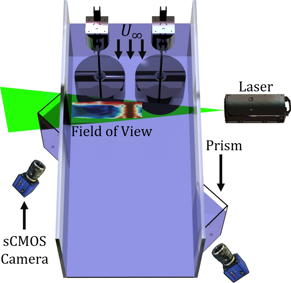
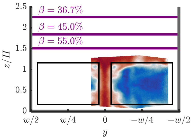
Two-camera, three-component particle image velocimetry is used to unobtrusively record the near-wake flow field in planes perpendicular to the flow (figure 5). Two cameras (Imager sCMOS 5.5 MPx, maximum 50 fps) with 35 mm and 60 mm lenses, are positioned on either side of the flume at approximately $45^{\circ}$ incidence to the image plane. The cameras are oriented perpendicular to water-filled acrylic prisms shown in figure 5, which are used to reduce refractive distortion from the angled camera positioning relative to the flume. Scheimpflug camera lens adaptors correct any residual focal distortions from angled fields of view (FoV). The FoV of each camera is focused on a domain centered behind one of the turbines and results in an overlapping 42.3$\times$27.7 cm² data collection region. The resulting FoV (figure 5) is positioned approximately 5.2 cm above the bottom of the flume and approximately 8.75 cm from the side wall to maximize capture of the flow through and around the array while reducing overexposure from laser scattering by solid boundaries, and encompasses the majority of the projected area of Turbine B, the bypass region above Turbine B, and the bypass region between the turbines. Although the FoV does not capture the full array, given the layout symmetry, the flow measured around Turbine B is expected to be descriptive of that near Turbine A. The entire flume is seeded with neutrally buoyant hollow glass spheres with a diameter of $\sim\!10\mu\mathrm{m}$ (Potters Industries Sphericel 110P8), and illumination is provided by a 532 nm Nd:YAG laser (EverGreen 200), which produces a light sheet approximately 2 mm thick.

The near-wake flow field is measured in vertical planes $0.6D$ and $1.5D$ downstream of the turbines’ axes of rotation, with the array moved in the streamwise direction to change the relative location of the vertical plane. We focus our analysis on the plane nearest to the array, at $0.6D$, with the flow fields at $1.5D$ provided in supplementary material. Flow field data in each plane are collected at $\beta=36.7\%$, $45.0\%$, and $55.0\%$ for tip-speed ratios of $\lambda=1.6$, $2.6$, $2.9$, and $3.6$ (all $\beta$) and $\lambda=4.2$ ($\beta=55.0\%$ only). These tip-speed ratios include the “optimal” $\lambda$ corresponding to maximum $C_{P}$ for $\beta=36.7\%$, $45.0\%$, and $55.0\%$, as well as $\lambda$ lower (“underspeed”) and higher (“overspeed”) than the optimal $\lambda$ at these blockage ratios, which are relevant for shedding power above the rated flow speed (Pao & Johnson, 2009). Data acquisition is synchronized with turbine phase ($\theta$), with images collected in $3^{\circ}$ increments at the $\lambda$ corresponding to maximum $C_{P}$ for $\beta=36.7\%$, $45.0\%$, and $55.0\%$, and $12^{\circ}$ increments for all other $\lambda$ cases. A total of 40 frames are collected at each phase and are averaged to reduce measurement noise. All phases are then averaged together to produce representative time-averaged fields.

LaVision Davis 10.2.1 software is used to acquire and process the PIV data. A dual-plane calibration target and self-calibration are employed. The resulting scale factor is 7.97 pix/mm with fitting errors of 0.81 and 0.92 pixels for each camera, respectively. A minimum filter subtracts background noise and an average polynomial filter using an interrogation window of 11$\times$11 pixels minimizes unsteady reflections from the free surface or near-blade regions. Vector calculation employs an initial $128\times 128$ interrogation window with a 50% overlap followed by four sequential reducing passes to $32\times 32$ pixels at a 75% overlap. After vector calculation, three passes of a universal outlier detection median filter (Westerweel & Scarano, 2005) removes vectors with a median normalized residual greater than 1.5 on a filter domain of $7\times 7$ vectors. These vectors were reinstated if their normalized residual was less than 2.5 and alternate correlation peaks had a higher residual. Groups with fewer than five vectors were removed.

3 Experimental Results

3.1 Array Performance

Figure 6: Time-averaged 6 $C_{P}$ and 6 $C_{T}$ as a function of $\beta$ and $\lambda$. The shaded regions indicate the interquartile range of the array- and cycle-averaged performance at each $\beta$ and $\lambda$ (the vertical span of the shaded region at each point is similar to the size of the markers for most operating conditions).

Time-average $C_{P}$ as a function of $\beta$ and $\lambda$ is shown in figure 6. In agreement with prior work in table 1, as $\beta$ increases, the maximum $C_{P}$ increases, the array produces power over a broader range of tip-speed ratios, and the optimal tip-speed ratio increases. Similarly, the time-averaged $C_{T}$ (figure 6) generally increases with $\beta$, particularly at higher blockage ratios. Above $\beta=33.4\%$, maximum $C_{P}$ exceeds the Betz limit, and above $\beta=50.0\%$, maximum $C_{P}$ exceeds unity. Such efficiencies are not violations of energy conservation since the definition of $C_{P}$ (Eq. 6) considers only the kinetic power that passes through the array projected area. This conventional definition neglects the contribution from the fluid’s potential energy, which is appreciably drawn down as $\beta$ and $C_{T}$ increase. As $\beta$ increases, a bounded efficiency metric may resemble the hydraulic efficiency of a hydropower turbine (such as that employed by Takamatsu et al. (1985) or McAdam et al. (2013a)) in which the available power is a function of volumetric flow rate through and the head drop across the rotor. This alternative efficiency metric is explored further in the supplementary material, but is sensitive to the resolution and accuracy of free surface measurements. Here, the conventional definitions of $C_{P}$ and $C_{T}$ facilitate comparison with prior studies, as well as consistency with LMADT—which is formulated using the definition of $C_{T}$ in Eq. 7.

Figure 7: Time-averaged 7 $C_{P}$ and 7 $C_{T}$ versus $\beta$ at constant $\lambda$. The data for each $\beta$ are interpolated at each $\lambda$ from the points in figure 6. The dashed lines represent the line of best fit through the data points corresponding to $\beta\leq 45.0\%$ at each $\lambda$.

When the array power and thrust coefficients are regressed against $\beta$ at constant tip-speed ratio, approximately linear relationships are revealed, which are shown for a subset of $\lambda$ in figure 7. Below a threshold value of $\lambda$ both $C_{P}$ and $C_{T}$ are independent of the blockage ratio and depend only on the tip-speed ratio, which corresponds to the collapsed regions of the $C_{P}-\lambda$ curves ($\lambda<1.6$) and $C_{T}-\lambda$ curves ($\lambda<1.2$) in figure 6. Similar relations are observed in prior work (Consul et al., 2013; Kolekar & Banerjee, 2015; Badshah et al., 2019). As $\lambda$ increases further, $C_{P}$ and $C_{T}$ vary linearly with the blockage ratio for $\beta\leq 45.0\%$ and moderate $\lambda$, which is emphasized by the linear regressions in figure 7. While similar linear relationships between the blockage ratio, power, and thrust have been previously identified in simulations of oscillating foils (Gauthier et al., 2016), axial-flow turbines (Kinsey & Dumas, 2017; Abutunis & Menta, 2022) and cross-flow turbines (Kinsey & Dumas, 2017), this is the first experimental demonstration of this trend. Finally, as $\beta$ and $\lambda$ increase further, these relationships become non-linear with performance increasingly sensitive to incremental changes in the blockage and tip-speed ratios, which is similar to narrower observations for $C_{P}$ by Gauthier et al. (2016)

3.2 Flow Fields

Figure 8: Time-averaged streamwise velocity $0.6D$ downstream of the array as function of $\beta$ and $\lambda$. Velocity measurements are normalized by the freestream velocity measured by the ADV. The black rectangles in each tile indicate the projected area of the turbines in the field of view. Flow fields corresponding to the optimal $\lambda$ for each blockage are outlined in purple (tiles 8 8, and 8).

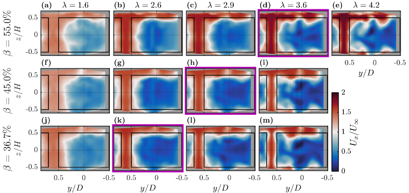
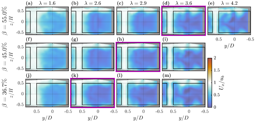
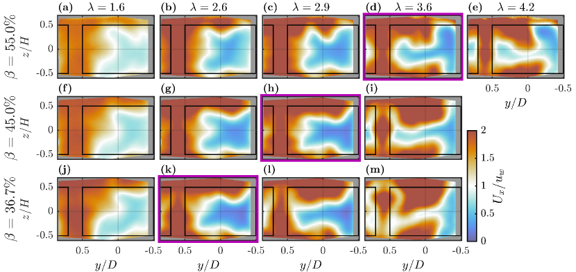
Figure 8 shows the normalized time-average streamwise velocity field $0.6D$ downstream of the array (i.e., within the near-wake) as a function of $\beta$ and $\lambda$. For each $\beta$ and $\lambda$, the velocity field is characterized by a wake region behind the turbines that is slower than the freestream ($U_{x}/U_{\infty}<1$, indicated by blue hues) and a bypass region above, below, and between the turbines where the flow is accelerated ($U_{x}/U_{\infty}>1$, indicated by red hues). We note that the bypass flow region between Turbine B and the flume side wall lies outside of the field of view, and we attribute the persistent region of decelerated flow below the turbine projected area at all $\lambda$ to obstruction of the flow by the test rig (figure 3).

Figure 9: Time-averaged normalized streamwise velocity profiles measured $0.6D$ downstream of the array for various $\beta$ at 9 $\lambda=1.6$, 9 $\lambda=2.6$, and 9 $\lambda=3.6$. The profiles correspond to the average velocity along the middle $70\%$ of the turbine blade span. Vertical gray rectangles correspond to the bypass region and delineate the relative turbine position and wake flow region (white).

Trends in the near-wake velocity with $\beta$ and $\lambda$ are more apparent when visualized as two-dimensional velocity profiles of the average velocity field over the middle $70\%$ of the blade span at each $y/D$ position, as shown in figure 9 for $\lambda=1.6$, $2.6$, and $3.6$ as a function of $\beta$. Ripples in the velocity profiles in the wake region are attributed to the passage of vortices shed from the blades during their downstream sweep. At $\lambda=1.6$ (figure 9), where array thrust varies weakly with $\beta$ (figure 7), $U_{x}/U_{\infty}$ increases slightly with $\beta$ throughout the entire profile, although the general shape of the velocity profile is constant. As $\lambda$ increases (figures 9 and 9), the turbines impart greater resistance on the flow and more fluid is diverted around them, which causes $U_{x}/U_{\infty}$ to increase in the bypass region (i.e., the gray shaded areas in figure 9) at all $\beta$. Similarly, as the blockage ratio increases at constant $\lambda$, the bypass velocity increases. $U_{x}/U_{\infty}$ at a given $\lambda$ also tends to increase in the wake region with $\beta$ since confinement increases the flow through the turbines. However, the increase in wake velocity is less pronounced than the corresponding increase in bypass velocity since momentum is extracted from the flow that passes through the turbines. Although the maximum bypass velocity (which occurs at the array centerline) increases with both the blockage ratio and the tip-speed ratio, $U_{x}/U_{\infty}$ decreases more rapidly away from the centerline at higher $\lambda$, as indicated by the narrowing of the peaks in the velocity profiles in figure 9 at all $\beta$ as $\lambda$ increases. Conversely, an increase in $\beta$ at constant $\lambda$ results in a more gradual reduction of $U_{x}/U_{\infty}$ away from the array centerline, which implies increased turbulent mixing between the bypass flow and the core flow through the turbine. As discussed by Nishino & Willden (2012a), this mixing between the bypass and core flows provides a secondary enhancement of power with increasing blockage by increasing the pressure drop across the rotor as a consequence of increasing velocity in the near-wake.

3.3 Free Surface Deformation

Figure 10: Time-averaged streamwise water depth profiles across Turbine B for various $\lambda$ at 10 $\beta=36.7\%$, 10 $\beta=45.0\%$, and 10 $\beta=55.0\%$. The farthest upstream measurement is taken at the center of the channel, whereas depth measurements in the vicinity of the array are directly upstream and downstream of the turbine (figure 3). Depth measurements at each streamwise location ($h_{x}$) are normalized by the far-upstream water depth ($h$) measured at the same $\beta$ and $\lambda$. The dashed lines indicate the extent of the turbine’s swept area.

The time-average streamwise free surface profile across Turbine B is shown in figure 10 at the same combinations of $\beta$ and $\lambda$ as for the flow fields in figure 8. For all $\beta$ and $\lambda$, a drop in the free surface is observed across the turbine, consistent with the pressure drop across the array from momentum extraction in an open-channel flow (Vogel et al., 2016). The magnitude of this drop (in this case, the difference between the measured water depths at $x/D=-1$ and $x/D=1$) tends to increase with $\beta$ for a given $\lambda$. However, as shown in Appendix A, the free surface drop behind the array also depends on the normalized submergence depth ($s/h$) which decreases with $\beta$ in these experiments (Section 2.2). Consequently, the free surface drop at higher $\beta$ is likely augmented by the closer proximity of the turbines to the free surface. The free surface drop across the turbine clearly increases with $\lambda$ at $\beta=55.0\%$ (figure 10), consistent with the monotonic increase in $C_{T}$ with $\lambda$ (figure 6). However, even though similar relationships between $C_{T}$ and $\lambda$ are observed for $\beta=36.7\%$ and $\beta=45.0\%$, the measured free surface drop at these blockages does not vary significantly with the tip-speed ratio for $\lambda\geq 2.6$, although the measured depth at $x/D=0.5$ does continuously decrease with the $\lambda$ for all $\beta$.

4 Evaluation of LMADT Accuracy for a Cross-flow Turbine Array

4.1 Model Overview

Figure 11: Linear momentum model for an actuator disk in open-channel flow defined by Houlsby et al. (2008) and adapted to the cross-flow turbine array nomenclature.

The performance, flow field, and free surface measurements described in Section 3 allow us to directly assess the accuracy of a one-dimensional linear momentum actuator disk theory (LMADT) description of the high confinement cross-flow turbine array. Given the equivalence between local and global blockage in the experimental setup (Section 2.3) and appreciable free surface deformation (figure 10), the open-channel LMADT model introduced by Houlsby et al. (2008) is most relevant. We note that, in the limiting case of negligible free surface drop across the turbine array ($Fr_{h}^{2}\rightarrow 0$), this formulation reduces to the well-known model of Garrett & Cummins (2007). Detailed derivations of the LMADT equation set are presented in Houlsby et al. (2008) and Houlsby & Vogel (2017).

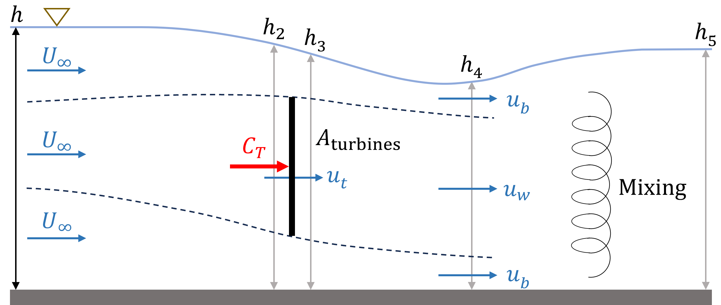
A schematic of the open-channel model, as applied to the present cross-flow turbine array, is shown in figure 11. The cross-flow turbine array is represented as a single actuator disk with the same blockage ratio and thrust coefficient as the array. For non-uniform turbine spacing, a theory that represents the individual turbines in the array as separate actuator disks would be required (e.g., Nishino & Willden, 2012b; Vogel et al., 2016; Dehtyriov et al., 2021). The flow upstream of the turbine is unidirectional, uniform, and subcritical with a velocity $U_{\infty}$ and a depth $h$. In response to momentum extraction by the turbine, the “core” flow in the streamtube that passes through the rotor slows from $U_{\infty}$ to $u_{t}$ just upstream of the rotor plane, and further decelerates to $u_{w}$ downstream of the turbine in the near-wake. To satisfy continuity, the fluid outside of this streamtube is accelerated from $U_{\infty}$ to $u_{b}$. The core wake velocity ($u_{w}$) and bypass velocity ($u_{b}$) are defined at a location downstream of the turbine where the pressure in the core and bypass flows is equal and hydrostatic. The flow is assumed to be axisymmetric and inviscid up to this location, downstream of which $u_{w}$ and $u_{b}$ mix. Far downstream, the flow is once again uniform, with reduced depth due to the energy extracted by the disk but higher velocity to maintain constant mass flux through the channel. This model qualitatively captures aspects of the experimentally observed wake and bypass velocities (figure 8). However, although LMADT models are widely used to represent turbine hydrodynamics in confined flows—most often as the basis for analytical blockage corrections (e.g., Bahaj et al., 2007; Whelan et al., 2009; Ross & Polagye, 2020a)—several of the underlying assumptions are violated. For example, the wake is assumed to be axisymmetric and to not mix with the bypass until static pressure has equilibrated between the core and bypass flows.

The implementation of the open-channel model used here follows that of Ross & Polagye (2020a), who reorganized Houlsby et al.’s original formulation into two equations from which $u_{w}$ and $u_{b}$ can be obtained numerically if $U_{\infty}$, $C_{T}$, $Fr_{h}$, and $\beta$ are known:

$$u_{w}=\frac{Fr_{h}^{2}u_{b}^{4}-(4+2Fr_{h}^{2})U_{\infty}^{2}u_{b}^{2}+8U_{\infty}^{3}u_{b}-4U_{\infty}^{4}+4\beta C_{T}U_{\infty}^{4}+Fr_{h}^{2}U_{\infty}^{4}}{-4Fr_{h}^{2}u_{b}^{3}+(4Fr_{h}^{2}+8)U_{\infty}^{2}u_{b}-8U_{\infty}^{3}}\ ,$$ (8)

$$u_{w}=\sqrt{u_{b}^{2}-C_{T}U_{\infty}^{2}}\ .$$ (9)

The velocity through the turbine, $u_{t}$, is then given as

$$u_{t}=\frac{u_{w}(u_{b}-U_{\infty})(2gh-u_{b}^{2}-u_{b}U_{\infty})}{2\beta gh(u_{b}-u_{w})}\ .$$ (10)

For the solutions to Eqs. 8, 9 and 10 to be physically valid, the core and bypass flows must be subcritical and satisfy $u_{b}>u_{t}>u_{w}$ and $u_{b}>U_{\infty}>u_{t}$.

The free surface profile in the vicinity of the array can also be calculated from the open-channel LMADT model. Houlsby et al. define five streamwise stations, $x_{1}-x_{5}$:

1. Far upstream, where the flow is undisturbed by the disk ($h_{1}$ = $h$; $U_{1}=U_{\infty}$);

2. Just upstream of the actuator disk ($h_{2}$; $U_{2}=u_{t}$);

3. Just downstream of the actuator disk ($h_{3}$; $U_{3}=u_{t}$);

4. Downstream of the actuator disk, where the static pressure in the core and bypass

5. flows is equal ($h_{4}$; $U_{4}$ = $u_{w}$ in the core flow; $U_{4}=u_{b}$ in the bypass); and

6. Far downstream of the disk, when the flow has fully mixed ($h_{5}$; $U_{5}$),

where $h_{1}$ through $h_{5}$ and $U_{1}$ through $U_{5}$ are the water depth and velocity, respectively, at each station. Once $u_{w}$, $u_{b}$, and $u_{t}$ have been calculated from Eqs. 8, 9 and 10, then $h_{4}$, $h_{3}$, and $h_{2}$ may be calculated following Houlsby et al. (2008) as

$$h_{4}=h+\frac{(U_{\infty}^{2}-u_{b}^{2})}{2g}\ \ ,$$ (11)

$$h_{3}=h_{4}+\frac{(u_{w}^{2}-u_{t}^{2})}{2g}\ \ ,$$ (12)

$$h_{2}=h+\frac{(U_{\infty}^{2}-u_{t}^{2})}{2g}\ \ .$$ (13)

The normalized net free surface drop across the channel from far upstream ($x_{1}$) to far downstream ($x_{5}$), $\frac{\Delta h}{h}$, is obtained by solving

$$\frac{1}{2}\left(\frac{\Delta h}{h}\right)^{3}-\frac{3}{2}\left(\frac{\Delta h}{h}\right)^{2}+\left(1-Fr_{h}^{2}+\frac{C_{T}\beta Fr_{h}^{2}}{2}\right)\frac{\Delta h}{h}-\frac{C_{T}\beta Fr_{h}^{2}}{2}=0\ \ ,$$ (14)

from which $h_{5}$ is obtained as

$$h_{5}=h\left(\frac{\Delta h}{h}\right)\ \ .$$ (15)

In our experiments, because the static pressure equilibrium point is unknown, $x_{4}$ is ambiguous, as are $x_{2}$ and $x_{3}$ due to the non-zero rotor “thickness”. In addition, the flume has insufficient length for the flow to fully mix downstream of the array, such that $x_{5}$ cannot be measured. Consequently, although $u_{b}$, $u_{w}$, and $u_{t}$ may be estimated from available measurements and $h_{2}$ through $h_{5}$ calculated, the exact streamwise positions of $x_{2}$ through $x_{5}$ relative to the experimental array are ambiguous.

4.2 Comparison between Experimental and Modeled Near-Wake Velocities

Figure 12: The 12 bypass velocities, and 12 wake velocities (all normalized by the freestream velocity) predicted by the open-channel LMADT model of Houlsby et al. (2008) from measurements of array thrust and flow conditions.

Using the measured values of $C_{T}$, $U_{\infty}$, $Fr_{h}$, and $\beta$, $u_{b}$ and $u_{w}$ are calculated at each $\lambda$ using Eqs. 8 and 9. The resulting analytically-predicted velocities are normalized by the freestream velocity in figure 12. Qualitatively, trends in near-wake velocities predicted by LMADT agree with trends in the experimental near-wake velocities (figure 8). At a given tip-speed ratio, both $u_{b}$ (figure 12) and $u_{w}$ (figure 12) increase with $\beta$ because confinement accelerates the flow through and around the turbine. As $\lambda$ increases, $u_{b}$ increases at all $\beta$ since thrust increases with $\lambda$ and more flow is diverted around the array, whereas $u_{w}$ decreases with $\lambda$ at all $\beta$ due to momentum extraction by the array. In agreement with experimental trends in the velocity profiles in figure 9, modeled $u_{b}$ increases more strongly with tip-speed ratio at higher blockage. We note that the modeled $u_{w}$ is always positive, indicating that the upper limit of the thrust coefficient for physically-valid solutions to open-channel LMADT (analogous to $C_{T}\leq 1$ for LMADT in unconfined flow) is not exceeded in these experiments.

Figure 13: Time-averaged streamwise velocities measured $0.6D$ downstream of the array at $\beta=36.7\%$, $45.0\%$, and $55.0\%$ and optimal $\lambda$, normalized by the corresponding 13-13 modeled bypass velocity, $u_{b}$, and 13-13 modeled wake velocity, $u_{w}$. The black rectangles indicate the projected area of the turbines in the field of view.

Figure 14: Time-averaged streamwise velocity profiles measured $0.6D$ downstream of the array normalized by the modeled bypass velocity at 14 $\beta=36.7\%$, 14 $45.0\%$, and 14 $55.0\%$ and various $\lambda$. The profiles shown correspond to the average velocity along the middle $70\%$ of the turbine blade span. Vertical gray rectangles correspond to the bypass region and delineate the relative turbine position and wake flow region (white).

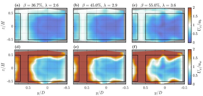
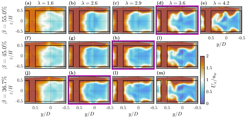
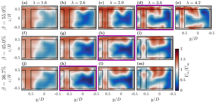
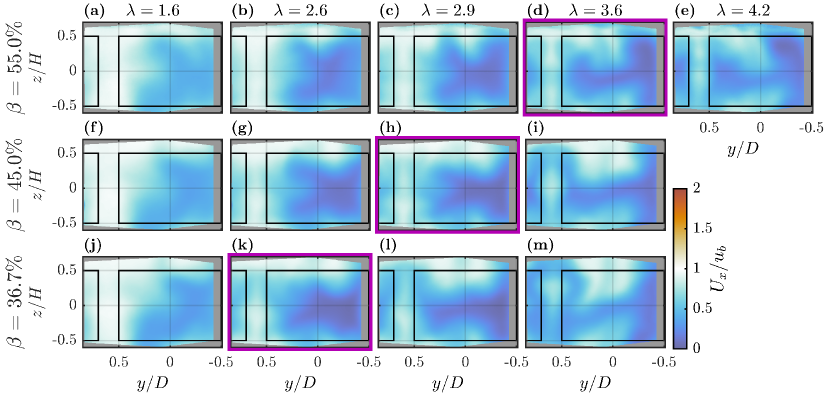
In figure 13, the time-averaged streamwise near-wake velocities at $\beta=36.7\%$, $45.0\%$, and $55.0\%$ and optimal $\lambda$ are normalized by $u_{b}$ and $u_{w}$, respectively. Blue hues correspond to experimental velocities lower than the LMADT-modeled value, red hues correspond to experimental velocities higher than the LMADT-modeled value, and white indicates agreement between the experimental and modeled velocities. The measured bypass velocity is well-predicted by LMADT, as indicated by the substantive white regions in figures 13, 13 and 13. As shown in the bypass-normalized velocity profiles in figure 14, the modeled $u_{b}$ tends to be slightly higher than experimental measurements at the array centerline, but are within approximately $8\%$ of the measured value for all $\beta$ and $\lambda$. In contrast, the measured wake velocities are lower than modeled wake velocities at all $\lambda$, and there is no substantive region of the flow that is well represented by $u_{w}$ (figures 13, 13 and 13). Flow fields normalized by $u_{b}$ and $u_{w}$ at other $\beta-\lambda$ combinations are provided as supplementary material.

Figure 15: Examples of non-idealities in the measured flow fields that are not present in the flow fields assumed by linear momentum theory, shown for the streamwise flow through a plane $0.6D$ downstream of the array operating at $\beta=36.7\%$, $45.0\%$, and $55.0\%$ and optimal $\lambda$. 15–15 Standard deviation of the measured streamwise velocity field, calculated as the standard deviation of the phase-average streamwise velocity field across all phases. 15–15 Time-averaged streamwise vorticity at the same location and conditions, calculated from the phase-averaged velocity fields and averaged across all phases. 15–15 Time-averaged turbulent kinetic energy (TKE) measured at the same location and conditions. To account for the inherent periodicity of cross-flow turbine wakes, the TKE field shown is obtained by calculating the TKE at each phase from the individual frames collected at that phase, then averaging the resulting fields across all phases.

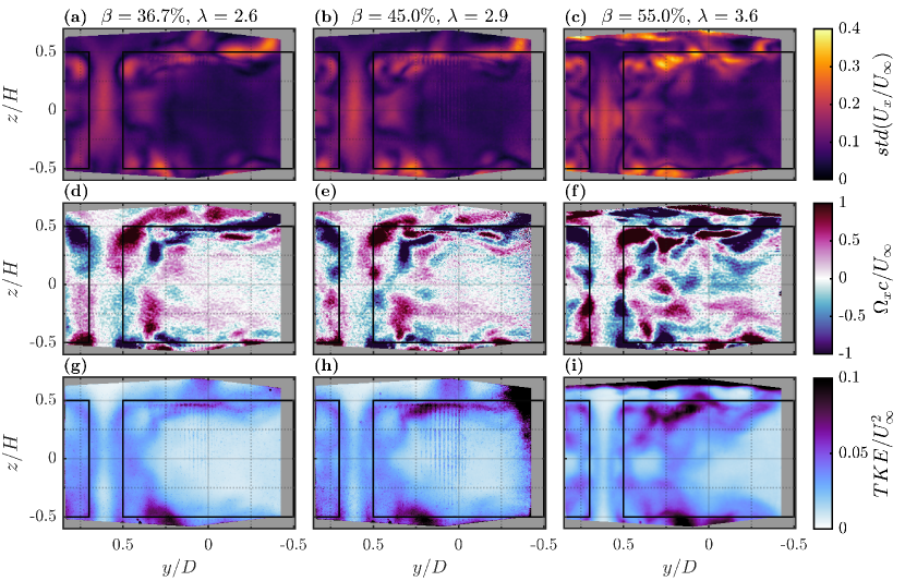
Although the time-averaged flow fields in figure 8 show distinct wake and bypass regions downstream of the array, the quantitative agreement between the modeled and measured bypass velocities is remarkable given the multiple violations of LMADT in the near-wake flow field. Examples of these non-idealities are highlighted at optimal tip-speed ratio for $\beta=36.7\%$, $45.0\%$ and $55.0\%$ in figure 15. First, unlike the uniform and one-dimensional flow assumed by the LMADT model, the flow in the near-wake varies in space and time, even within the bypass and wake regions (figures 15, 15 and 15). Second, the flow is also rotational (figures 15, 15 and 15): the periodic hydrodynamics of cross-flow turbines give rise to dynamic stall vortices that are shed into the region between the two turbines, and strong tip vortices form along the top and bottom of the turbine projected area. The asymmetric vorticity produced by these sources is expected to drive flow toward the center of each turbine, contributing to wake asymmetry (Bachant & Wosnik, 2015; Ryan et al., 2016). Third, as suggested by the velocity profiles in figure 9 and the turbulent kinetic energy (TKE) in the near-wake (figures 15, 15 and 15), mixing occurs within the shear layer between the bypass flow and the turbine wake, consistent with a co-flowing turbulent jet. In contrast, the LMADT model assumes that the core and bypass flows do not mix until further downstream from where $u_{b}$ is defined (figure 11). This near-wake mixing necessarily reduces the bypass velocity, which may explain why the modeled bypass velocity is slightly higher than the measured bypass velocity at the array centerline (figure 14). Finally, as described in Section 4.1, $u_{b}$ is specified at a location downstream of the turbines where the static pressure is equal in the wake and bypass flows. Although it is unknown whether this condition is satisfied $0.6D$ downstream of the array, $u_{b}$ is less descriptive of the measured bypass flow further downstream ($1.5D$, provided as supplementary material).

4.3 Comparison between Experimental and Modeled Free Surface Deformation

Figure 16: Modeled free-surface profile at various stations along the channel predicted using the open-channel LMADT model of Houlsby et al. (2008) and the measured $C_{T}$, $h$, and $U_{\infty}$ for 16 $\beta=36.7\%$, 16 $\beta=45.0\%$, and 16 $\beta=55.0\%$ for various $\lambda$. The dashed black line indicates the relative location of the array, represented in the linear momentum model as a thin actuator disk.

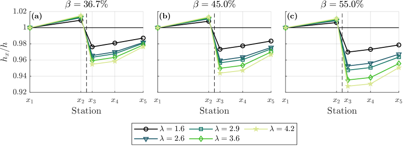
For comparison with the measured free surface profiles in figure 10, the theoretical free surface profiles are shown for the same $\beta$ and $\lambda$ in figure 16. As noted in Section 4.1, we emphasize that the exact locations of $x_{2}-x_{4}$ relative to the physical array are ambiguous and that $x_{5}$ is likely further downstream than can be measured given the finite length of the flume downstream of the turbines. Consequently, the locations of $x_{1}$ through $x_{5}$ relative to the actuator disk model of the array shown in figure 16 are qualitative. With these caveats, we consider the measured trends in free surface deformation relative to trends in the modeled values. For all $\beta$, the modeled water depth just upstream of the actuator disk ($h_{2}/h$) increases continuously with $\lambda$. Similarly, the immediate static head drop across the actuator disk ($(h_{3}-h_{2})/h$) and the total free surface drop across the channel ($\Delta h/h$) increase continuously with both $\lambda$ and $\beta$.

This analytical result is consistent with a direct relationship between the pressure drop across the array (i.e., the thrust coefficient) and a drop in the free surface across the array, but conflicts with measured free surface profiles in figure 10. Although, as previously noted, the measured $C_{T}$ increases continuously with $\lambda$ at all $\beta$, the measured free surface drop across the turbines at $\beta=36.7\%$ (Figure 10) and $45.0\%$ (Figure 10) does not depend significantly on $\lambda$ for $\lambda\geq 2.6$. This may suggest that LMADT is not fully descriptive of the evolution of the free surface in the vicinity of high blockage turbines, although the limited spatial and temporal resolution of the instrumentation employed precludes a more comprehensive characterization of the free surface dynamics in this data set. Finally, we do experimentally observe trends consistent with modeled deformation for $\beta=55.0\%$.

4.4 Bluff-Body Scaling of Performance Data

Figure 17: Time-averaged array performance from figure 6 scaled by 17 the corresponding analytical bypass velocities (figure 12) and 17 the unconfined freestream velocity calculated using Eq. 19.

Given that open-channel LMADT is descriptive of the measured bypass flow across a range of array operating conditions, we turn to the question of whether LMADT can also be descriptive of the measured array performance. In prior work, LMADT has been most commonly used in analytical blockage corrections to estimate unconfined performance from measurements or simulations of confined operation (e.g., Bahaj et al., 2007; Chen & Liou, 2011; Kinsey & Dumas, 2017; Ross & Polagye, 2020a). However, since a perfect blockage correction would be expected to collapse the $C_{P}$ and $C_{T}$ measured at different blockage ratios (e.g., figure 6) onto common unconfined $C_{P}-\lambda$ and $C_{T}-\lambda$ curves, such corrections imply not just a connection between confined and unconfined performance, but rather a broader self-similarity in turbine performance across blockage ratios. Here, we explore such self-similar aspects of array performance with a focus on the significance of the bypass flow.

To investigate the relationship between the bypass flow and array performance, we apply a method introduced by Whelan et al. (2009) and based on the bluff-body theory of Maskell (1963) to scale the experimental array performance by the corresponding bypass velocities predicted from LMADT:

$${C_{P}}^{b}=C_{P}{\left(\frac{U_{\infty}}{u_{b}}\right)}^{3},$$ (16)

$${C_{T}}^{b}=C_{T}{\left(\frac{U_{\infty}}{u_{b}}\right)}^{2},$$ (17)

$${\lambda}^{b}=\lambda\left(\frac{U_{\infty}}{u_{b}}\right).$$ (18)

As shown in figure 17, the resulting ${C_{P}}^{b}-{\lambda}^{b}$ and ${C_{T}}^{b}-{\lambda}^{b}$ curves collapse across the tested blockage and tip-speed ratios, indicating that array power, thrust, and their relationship to rotation rate scale with the bypass velocity for these experimental conditions. Consequently, one may interpret $u_{b}/U_{\infty}$ as a similarity variable for array performance that is well-predicted by linear momentum theory. Some spread in the bypass-scaled thrust curves is observed (maximum $\Delta{C_{T}}^{b}\approx 0.06$), particularly at lower $\lambda^{b}$, but the bypass-scaled power curves exhibit excellent collapse at all $\lambda^{b}$ (maximum $\Delta{C_{P}}^{b}\approx 0.016$). As $u_{b}$ is calculated using the measured $C_{T}$ in Eqs. 8 and 9, it is not surprising that $C_{T}$ scales with $u_{b}$. However, given that measurements of $C_{P}$ are not involved in the calculation of $u_{b}$, the collapse in the ${C_{P}}^{b}-{\lambda}^{b}$ curves is notable, especially since the rotation, torque, and lateral forces experienced by the cross-flow turbines are all neglected in LMADT.

The hydrodynamics that underlie the connection between the bypass velocity and array performance are well-described by Nishino & Willden (2012a). In summary, as $\beta$ increases, the velocity of the fluid bypassing the array increases (figures 9 and 12). Since energy is conserved in the bypass flow, this acceleration corresponds to an increased pressure drop in the bypass. To satisfy pressure equilibrium between the core and bypass flows both far upstream and far downstream, the pressure drop in the core flow through the turbines must also increase. In an open-channel flow, this pressure drop manifests as a free surface drop along the channel. As $\beta$ increases, the increased pressure drop across the array accelerates the flow through the turbines, which increases power and thrust at higher blockage.

This connection between the bypass velocity and array performance parallels the theory of Maskell (1963), who proposed that the drag force on a bluff body in confined flow is related to the flow bypassing the body, not the undisturbed upstream condition. Assuming a uniform and unidirectional inflow and axisymmetric wake, Maskell developed a model for this behavior by combining conservation of momentum in the flow outside the wake with an empirical relationship for wake contraction due to confinement, and demonstrated through experiments that this model was descriptive of the drag on square flat plates at relatively low blockage ratios ($\beta\leq 10\%$). Maskell leveraged this relationship to propose a blockage correction that predicted the drag on a bluff body in unconfined flow given thrust measurements on the same body in a wind tunnel. As the wake characteristics of wind and water turbines resemble those of a bluff body under certain conditions (Medici & Alfredsson, 2006; Chamorro et al., 2012; Araya et al., 2017), several subsequent studies have extended Maskell’s theory. While some have directly applied Maskell’s flat plate blockage correction to turbine performance data, (Zilic de Arcos et al., 2020; Zhang et al., 2023), others have adapted this theory to specific turbine designs through analogous empirical relationships (Alexander & Holownia, 1978; Ross & Altman, 2011; Jeong et al., 2018; Zhang et al., 2023).

Whelan et al. (2009) were the first to combine the core idea of Maskell’s theory—that the thrust on a bluff body in confined flow scales with the bypass flow—with LMADT to develop a blockage correction for “highly” loaded turbines. Rather than directly implementing Maskell’s blockage correction, Whelan et al. utilized an open-channel LMADT model to calculate the expected $u_{b}$ from axial-flow turbine thrust measurements at high blockage ($\beta=64\%$), and utilized Eqs. 17 and 18 to scale the measured thrust coefficients and tip-speed ratios by this bypass velocity. The resulting ${C_{T}}^{b}-{\lambda}^{b}$ data agreed closely with the unconfined thrust coefficients predicted for the same turbine simulated using blade element momentum (BEM) theory. Kinsey & Dumas (2017) applied the same correction to CFD-simulated thrust data for a cross-flow turbine at $\beta=13\%$, $25\%$, and $51\%$ with $u_{b}$ calculated via closed-channel LMADT. The resulting ${C_{T}}^{b}-\lambda^{b}$ curves yielded better agreement with the simulated unconfined thrust coefficients than was obtained with the popular Barnsley & Wellicome (1990) blockage correction. While Whelan et al. left open the question of whether power could be similarly corrected, Ross & Polagye (2020a) introduced Eq. 16, used the LMADT model of Houlsby et al. (2008) to calculate $u_{b}$, and scaled the corresponding performance data for both an axial-flow turbine ($\beta=2\%$ and $35\%$) and cross-flow turbine ($\beta=3\%$ and $36\%$). However, in contrast to Whelan et al. and Kinsey & Dumas, at tip-speed ratios beyond optimal ($\lambda>5$ for axial-flow, $\lambda>1.85$ for cross-flow) Ross & Polagye observed moderately poor agreement between the measured low-blockage turbine performance and ${C_{P}}^{b}$ and ${C_{T}}^{b}$ calculated from high-blockage turbine performance. Relative to prior work, the bypass-scaled power and thrust coefficients in figure 17 exhibit the strongest collapse across blockages observed to date, and highlight the similarities between array hydrodynamics and bluff-body dynamics for a wide range of high-blockage operating conditions.

Since the scalings in Eqs. 16, 17 and 18 are typically interpreted as a Maskell-inspired bluff-body blockage correction, it is relevant to compare the bypass-scaled performance (figure 17) to that obtained via a “standard” LMADT blockage correction based on the theory of Glauert (1935), in which it is assumed that the thrust on the turbine responds to the velocity through the turbine ($u_{t}$). Using the LMADT-modeled values of $u_{t}$ from Eq. 10, the unconfined freestream velocity, ${U_{\infty}}^{\prime}$, that yields the same $u_{t}$ and dimensional thrust on the array in unconfined flow as in the confined system is given as

$${U_{\infty}}^{\prime}=\frac{U_{\infty}\left((u_{t}/U_{\infty})^{2}+C_{T}/4\right)}{u_{t}/U_{\infty}}\ .$$ (19)

The unconfined power coefficient (${C_{P}}^{\prime}$), thrust coefficient (${C_{T}}^{\prime}$), and tip-speed ratio ($\lambda^{\prime}$) are then calculated using Eqs. 16, 17 and 18 with ${U_{\infty}}^{\prime}$ in place of $u_{b}$. As shown in figure 17, up to ${C_{T}}^{\prime}\approx 1$, the ${C_{P}}^{\prime}-\lambda^{\prime}$ and ${C_{T}}^{\prime}-\lambda^{\prime}$ curves exhibit similar collapse across blockages to bluff-body scaling (maximum $\Delta{C_{P}}^{\prime}\approx 0.018$; maximum $\Delta{C_{T}}^{\prime}\approx 0.04$), with the values of ${C_{P}}^{\prime}$ and ${C_{T}}^{\prime}$ generally exceeding those of ${C_{P}}^{b}$ and ${C_{T}}^{b}$ at comparable re-scaled tip-speed. However, for LMADT in unconfined flow, the thrust coefficient cannot exceed unity as this implies reversed flow in the turbine wake. Thus, above the $\lambda^{\prime}$ corresponding to ${C_{T}}^{\prime}\approx 1$, only non-physical solutions exist, and the unconfined efficiency and thrust coefficient curves no longer collapse. Given this constraint on ${C_{T}}^{\prime}$, a key advantage of Maskell-inspired bluff-body scaling over a conventional LMADT blockage correction is the ability to describe the performance of high-blockage turbines over a wider range of confined $C_{T}$, and thus a wider range of $\beta$ and $\lambda$.

In the present work, measurements of array performance at $\beta\approx 0\%$ are not available, such that the accuracy of Eqs. 16, 17 and 18 for predicting unconfined performance cannot be assessed directly. However, we expect this Maskell-inspired scaling relationship to describe self-similar array performance only under conditions where turbine dynamics resemble those of a bluff body. While the results in this study demonstrate this is likely the case for $\beta=30-55\%$, Araya et al. (2017) showed that cross-flow turbine wakes at even lower blockage ($\beta=20\%$) resemble those of a solid cylinder as both the tip-speed ratio and rotor solidity increase. Consequently, we hypothesize that the range of blockage ratios over which bluff-body scaling can capture self-similar aspects of array performance depends on operating condition and rotor geometry. Based on the results of Araya et al. (2017), we expect the lower threshold of $\beta$ at which bluff-body scaling is applicable may depend on the “dynamic solidity” of the turbine or array, which increases with increasing tip-speed ratio and rotor solidity. This may explain why the ${C_{T}}^{b}-\lambda^{b}$ curves in figure 17 increasingly collapse as $\lambda$ (and thus, $C_{T}$) increases, and is consistent with Whelan et al.’s (2009) original framing of Eqs. 17 and 18 as a blockage correction for highly-loaded turbines. Similarly, the poorer agreement between bluff-body scaled performance at $\beta=36\%$ and low-blockage performance at $\beta=3\%$ observed by Ross & Polagye (2020a) (who used a cross-flow turbine with similar solidity to this study) suggests limitations of bluff body scaling for describing low-blockage or unconfined performance.

5 Prediction of Confined Performance

The self-similar array performance yielded by Maskell-inspired bluff-body scaling provides a pathway for predicting performance at different blockages from measurements or simulations at another. For example, such information would be useful for describing time-varying performance in a tidal channel with changing water depth and, therefore, blockage. Although “correcting” performance to non-zero blockages using LMADT is briefly mentioned in prior work (e.g., Steiros et al., 2022; Dehtyriov et al., 2023), there have been limited demonstrations of such methods and we are unaware of any details describing the implementation. Whelan et al. (2009) applied their Maskell-inspired bluff-body blockage correction in reverse to predict the thrust coefficients of a turbine at $\beta=64\%$ from unconfined thrust calculated from BEM, but did not detail the procedure or quantify prediction accuracy. Kinsey & Dumas (2017) proposed an empirical forecasting method based on their observation that both the power and thrust coefficients exhibit approximately linear relationships with $\beta$ at constant $\lambda$ (similar to that in figure 7). Specifically, at several $\lambda$, Kinsey & Dumas develop a linear regression for confined performance from simulations at $\beta=20\%$ and the corresponding performance at $\beta=0\%$ estimated using the LMADT blockage correction of Barnsley & Wellicome (1990). Performance at other $\beta$ was then obtained by interpolation or extrapolation. Although this method was able to accurately predict the power and thrust coefficients at $\beta=10\%$, predictions were less accurate for extrapolation to $\beta\geq 50\%$ where the $C_{T}-\beta$ and $C_{P}-\beta$ relationships are expected to be less linear.

Here, a method for forecasting confined performance based on Houlsby et al.’s LMADT model and the Maskell-inspired bluff-body relationship between turbine performance and the bypass velocity is described. We expect that this approach is likely similar to that employed by Whelan et al. (2009). Consider a turbine in a channel (or an array of equally-spaced turbines spanning the channel width) with known performance at blockage ratio $\beta_{1}$ and Froude number $Fr_{h}$. At a given operating condition (e.g., $\lambda_{1}$) the turbine’s thrust coefficient is $C_{T,1}$ and bypass velocity is $u_{b,1}$. As for Glauert-derived blockage corrections, for the same turbine or array operating at a different blockage ratio, $\beta_{2}$, assume that there is a freestream velocity, $U_{\infty,2}$, that yields the same dimensional thrust on the turbine as at $\beta_{1}$ and $U_{\infty,1}$:

$$T_{1}=T_{2}\ .$$ (20)

Therefore,

$$C_{T,2}=C_{T,1}{\left(\frac{U_{\infty,1}}{U_{\infty,2}}\right)}^{2}\ .$$ (21)

Since the thrust on the turbine scales with the bypass velocity in a Maskell-inspired approach, equal thrust at $\beta_{1}$ and $\beta_{2}$ requires equal bypass velocity:

$$u_{b,1}=u_{b,2}=u_{b}\ .$$ (22)

Therefore, $C_{T,2}$ can be calculated from Eq. 21 if the value of $U_{\infty,2}$ that yields $u_{b}$ at $\beta_{2}$ can be determined. In other words, $C_{T,1}$ and $C_{T,2}$ are connected through a common value of ${C_{T}}^{b}$ when Maskell-inspired bluff-body scaling is applied as

$${C_{T}}^{b}=C_{T,1}{\left(\frac{U_{\infty,1}}{u_{b}}\right)}^{2}=C_{T,2}{\left(\frac{U_{\infty,2}}{u_{b}}\right)}^{2}\ .$$ (23)

Since rotor power also scales with the bypass velocity, $C_{P,2}$ is given as

$$C_{P,2}=C_{P,1}{\left(\frac{U_{\infty,1}}{U_{\infty,2}}\right)}^{3}\ .$$ (24)

Finally, assuming constant rotation rate (i.e., $\omega_{1}=\omega_{2}$),

$$\lambda_{2}=\lambda_{1}{\left(\frac{U_{\infty,1}}{U_{\infty,2}}\right)}\ .$$ (25)

In Eqs. 21 and 24, it is implicitly assumed that $\rho_{1}$ = $\rho_{2}$ (and thus, $\nu_{1}$ = $\nu_{2}$), which implies a difference in the freestream $Re_{D}$ (Eq. 4) between $\beta_{1}$ and $\beta_{2}$. However, the Reynolds number based on the bypass velocity ($u_{b}D/\nu$) remains constant. We note that the inability of LMADT to describe $u_{w}$ and, presumably, $u_{t}$ for relatively high confinement is not a limitation here, since LMADT is able accurately model the relationship between $\beta$, $C_{T}$, and $u_{b}/U_{\infty}$.

Figure 18: Flowchart describing the procedure for forecasting performance at $\beta_{2}$ based on performance at $\beta_{1}$, assuming constant Froude number between $\beta_{1}$ and $\beta_{2}$. Gray boxes indicate known or specified inputs, yellow circles/ovals indicate equation solving, blue boxes indicate quantities associated with bluff-body scaling, and green boxes indicate the outputs at $\beta_{2}$. The dashed arrows indicate steps where iteration is required.

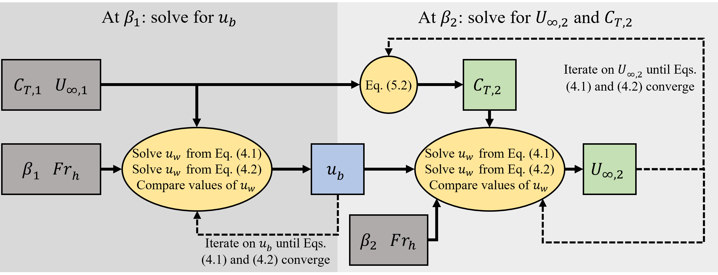
Using $u_{b}$ as a bridge between $\beta_{1}$ and $\beta_{2}$, LMADT can be used to calculate $U_{\infty,2}$ from known quantities at $\beta_{1}$. The procedure for calculating $U_{\infty,2}$ using the LMADT model of Houlsby et al. (2008) is outlined in figure 18. Here, we assume that the Froude numbers at $\beta_{1}$ and $\beta_{2}$ are constant and subcritical as for the experimental data, although constant Froude number is not mathematically required to utilize this method. First, $u_{b}$ is determined at $\beta_{1}$ by numerically solving Eqs. 8 and 9, using $C_{T,1}$, $U_{\infty,1}$, and $Fr_{h}$ as inputs. Next, a reasonable value of $U_{\infty,2}$ is guessed (e.g., $U_{\infty,2}=U_{\infty,1}$), from which a corresponding $C_{T,2}$ is calculated from Eq. 21. Equations 8 and 9 are then solved separately for $u_{w}$ at $\beta_{2}$ using $u_{b}$, $Fr_{h}$, and the guesses for $U_{\infty,2}$ and $C_{T,2}$. The resulting values of $u_{w}$ are compared, and this process is iterated with a new guess for $U_{\infty,2}$ until the value of $U_{\infty,2}$ that minimizes the difference between Eq. 8 and Eq. 9 is determined. With $U_{\infty,2}$ known, $C_{T,2}$, $C_{P,2}$ and $\lambda_{2}$ may be calculated from $C_{T,1}$, $C_{P,1}$, and $\lambda_{1}$ via Eqs. 21, 24 and 25. Note, however, that $C_{T,1}$ is the only performance metric at $\beta_{1}$ that influences the value of $U_{\infty,2}$.

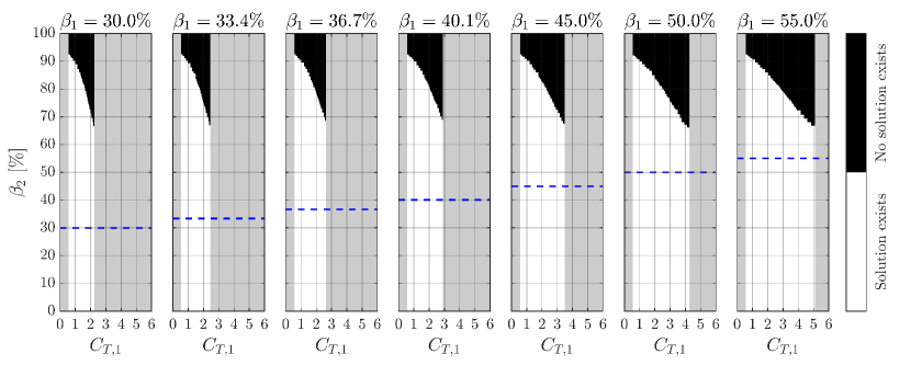
In the limiting case of $\beta_{2}\rightarrow 0$, $U_{\infty,2}\rightarrow u_{b}$ since the freestream velocity and bypass velocity are equal in unconfined flow. Consequently, Eqs. 21, 24 and 25 revert to Eqs. 16, 17 and 18 corresponding to a Maskell-inspired blockage correction (figure 17) with the implicit assumption that a bluff-body model is still representative of turbine dynamics at low blockage. Conversely, as $\beta_{2}\rightarrow 1$, the solution space is constrained by the requirements of equal bypass velocity and $Fr_{h}<1$ at $\beta_{1}$ and $\beta_{2}$, such that physically meaningful subcritical solutions at $\beta_{2}$ do not exist for all $\beta_{1}$ and $C_{T,1}$. The maximum value of $\beta_{2}$ at which a physical solution can be obtained depends on $C_{T,1}$, $\beta_{1}$, and the Froude numbers at $\beta_{1}$ and $\beta_{2}$; a visual representation of this limit for the experimental data is provided as supplementary material. However, for the performance data in this study, physically meaningful solutions exist for all practically-achievable blockages (i.e., $\beta_{2}\leq 65\%$).

Figure 19: 19-19 Predicted thrust coefficient and 19-19 error between the predicted thrust coefficient and measured thrust coefficient ($C_{T,0}$, shown as the gray lines in 19-19) for $\beta_{2}=30.0\%$, $45.0\%$, and $55.0\%$. Color indicates the difference between the blockage ratio of the performance data that was used to make each prediction ($\beta_{1}$) and the target blockage ratio ($\beta_{2}$). Note the different axes limits in 19-19.

Figure 20: 20-20 Predicted efficiency and 20-20 error between the predicted efficiency and measured efficiency ($C_{P,0}$, shown as the black lines in 20-20) for $\beta_{2}=30.0\%$, $45.0\%$, and $55.0\%$. Color indicates the difference between the nominal blockage ratio of the performance data that was used to make each prediction ($\beta_{1}$) and the target blockage ratio ($\beta_{2}$). Note the different axes limits for each $\beta_{2}$ in 20-20.

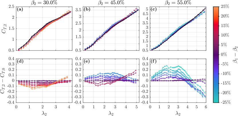
To quantify the effectiveness of this forecasting method, the measured array performance at $\beta_{1}=30.0\%-55.0\%$ (figure 6) is used to predict array performance at $\beta_{2}$ where measurements are also available. The resulting $C_{T,2}$ and $C_{P,2}$ at each operating point are then compared to the experimentally measured performance (denoted as $C_{T,0}$ and $C_{P,0}$) at each $\beta_{2}$. The predicted thrust coefficients at $\beta_{2}=30.0\%$, $45.0\%$ and $55.0\%$ and the corresponding difference between the predicted and measured thrust coefficients are given in figure 19. The measured thrust coefficients are predicted within $\sim\!0.2$ at $\beta_{2}=30.0\%$ and $45.0\%$ (figures 19 and 19) and within $\sim\!0.3$ at $\beta_{2}=55.0\%$ (figure 19). In general, the magnitude of the thrust prediction error increases with the difference between $\beta_{1}$ and $\beta_{2}$ (i.e., predictions further from the starting blockage are less accurate), and the absolute prediction error tends to grow as $\beta_{2}$ increases for the same difference between $\beta_{1}$ and $\beta_{2}$. In relative terms, these errors are appreciable at lower $\lambda_{2}$ where $C_{T}$ is relatively low, but decline for higher $\lambda_{2}$. Since the foundation of this forecasting method is Maskell-inspired bluff-body scaling (Eqs. 16, 17 and 18), the differences in the predicted $C_{T,2}$ across $\beta_{1}$ are driven by differences in ${C_{T}}^{b}$ across $\beta_{1}$. Thus, the shapes and relative positions of the ${C_{T}}^{b}-\lambda^{b}$ curves across $\beta_{1}$ (figure 17) dictate the shapes and relative positions of the resulting $C_{T,2}-\lambda_{2}$ curves when scaled to $\beta_{2}$ (figures 19, 19 and 19). For the current data set, at low to moderate tip-speed ratios this corresponds to underpredicted $C_{T,2}$ if $\beta_{1}>\beta_{2}$ and overpredicted $C_{P,2}$ if $\beta_{1}<\beta_{2}$, except at relatively high $\lambda$ when this trend inverts.

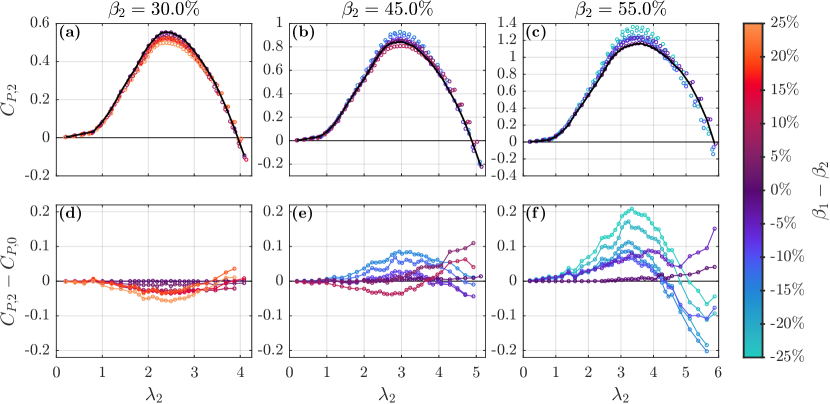
The corresponding predicted power coefficients and prediction error are shown in figure 20. The measured power coefficients are predicted within $\sim\!0.05$ at $\beta_{2}=30.0\%$ (figure 20), $\sim\!0.1$ at $45.0\%$ (figure 20), and $\sim\!0.2$ at $\beta_{2}=55.0\%$ (figure 20). The greatest prediction error tends to occur near the performance peak and at tip-speed ratios well beyond the optimal operating point. However, the tip-speed ratio corresponding to maximum performance is well-predicted (figures 20, 20 and 20). Since only the thrust influences the outcome of the bluff-body forecasting procedure, trends in the $C_{P,2}-\lambda_{2}$ curves with $\beta_{1}$ resemble those for the ${C_{T}}^{b}-\lambda^{b}$ curves.

The proposed forecasting method combines linear momentum theory and the bluff-body theory of Maskell to allow for analytically predicting confined turbine performance from experimental or simulation data. However, since this method utilizes $u_{b}$ as a link between $\beta_{1}$ and $\beta_{2}$, the prediction accuracy depends on whether the bypass velocity is descriptive of array performance at both $\beta_{1}$ and $\beta_{2}$. Consequently, the effectiveness of this forecasting scheme outside of the tested range of $\beta$ is unknown, and the method is likely less accurate when turbine dynamics depart from a bluff-body model. If there exists a transitional condition at which both a Maskell-inspired LMADT scaling (figure 17) and traditional Glauert-derived LMADT scaling (figure 17) provide similar results, then the use of a hybrid method that translates between these flow regimes might allow for forecasting performance across a wider ranges of blockages. However, the existence of such a transitional condition is speculative.

6 Conclusions

This research investigates the performance and near-wake flow fields of a cross-flow turbine array at the upper end of practically achievable blockage ratios and demonstrates the potential of theoretical frameworks to describe the dynamics of real turbines under these conditions. The performance and near-wake flow field of a two-turbine array were experimentally characterized over a wide range of operating conditions at array blockage ratios from $30\%$ to $55\%$, holding other non-dimensional flow parameters constant to isolate blockage effects. The observed array performance supports the trends observed in prior work while providing a uniquely high-resolution view of the manner in which performance changes with the blockage ratio at relatively high confinements. This highlights relatively subtle trends, such as linear behavior of both the power and thrust coefficients with blockage for low-to-moderate $\beta$ and $\lambda$. Similarly, the measured near-wake velocity fields quantitatively illustrate how the wake and bypass flows change with the blockage and tip-speed ratios. Critically, this work provides an openly-available set of experimental performance and flow-field data for cross-flow turbines at high blockage, which will aid in the validation of numerical simulations and reduced-order models that seek to examine confinement effects and inform the design of full scale systems that can exploit these physics.

A key outcome of this work is the demonstration that linear momentum actuator disk models can quantitatively describe aspects of real turbine arrays in highly confined flows. It is shown that, at a location $0.6$ turbine diameters downstream of the array, the velocity of the flow bypassing the array measured using PIV is well represented by the bypass velocity predicted from the open-channel LMADT model of Houlsby et al. (2008) with the measured array thrust coefficients and flow conditions as inputs. This result was confirmed for a wide range of blockages and tip-speed ratios, and the bypass velocity calculated from LMADT falls within approximately $8\%$ of the measured velocity between the turbines at the array centerline at all conditions. The residual deviation between modeled and measured bypass velocities may be a consequence of near-wake mixing that is neglected in LMADT. Following Whelan et al. (2009) and inspired by the bluff-body theory of Maskell (1963), scaling the array power and thrust coefficients by this analytical bypass velocity collapses these coefficients across the tested blockage and tip-speed ratios. These results highlight similar dynamics between high-blockage turbine arrays and bluff bodies, and demonstrate that, despite their inherent simplicity, LMADT models can effectively model aspects of the flow around non-ideal turbines in confined flows and provide insights into the salient hydrodynamics that govern their performance. Leveraging the connection between array performance and the bypass velocity, an analytical forecasting method based on LMADT is presented by which known turbine performance at one confinement ($\beta_{1}$) can be used to predict turbine performance at a different confinement ($\beta_{2}$) with moderate accuracy. The presented forecasting method provides a pathway for estimating turbine performance under confined conditions based on the dominant dynamics of high-blockage arrays. As such, we expect the broader applicability of this method and accuracy as a blockage correction to be influenced by factors such as rotor geometry and rotation rate that influence the similarity between turbine and bluff body dynamics (Araya et al., 2017).

Although this work focuses on cross-flow turbines, the characteristic fluid dynamics of confinement are not exclusive to this archetype, and the analytical models employed are agnostic to turbine geometry. However, the design of the rotor is expected to influence how these characteristic dynamics change with blockage and the tip-speed ratio (Schluntz & Willden, 2015), such that the effectiveness of Maskell-inspired bluff-body scaling and forecasting likely depend on turbine geometry and operating condition. It is recommended that future work explore the broader application of these analytical methods to turbines at lower confinement, as well as to different turbine designs. Additionally, although this work focuses on the time-averaged array performance and near-wake flow fields, the unsteady fluid dynamics of cross-flow turbines also inform their performance and the properties of the near-wake. Future research should examine how the phase-resolved performance of cross-flow turbines develops with confinement, and how these dynamics influence the temporal and spatial evolution of the flow field in the near- and far-wake regions.

[Acknowledgements]The authors would like to thank Gregory Talpey, Gemma Calandra, and Corey Crisp for their assistance in commissioning the high-confinement test-rig, as well as help with data collection. Abigale Snortland, Hannah Ross, Jennifer Franck, and Mukul Dave are acknowledged for insightful conversations regarding the results in this work. We are grateful to the Alice C. Tyler Charitable Trust for upgrades to the experimental flume, including closed loop heating and cooling.

[Funding]This work was supported by the United States Advanced Research Projects Agency – Energy (ARPA-E) under award number DE-AR0001441.

[Declaration of interests]The authors report no conflict of interest.

[Data availability statement] The data that support the findings of this study are openly available in the Dryad data repository at https://doi.org/10.5061/dryad.dfn2z35b5 (DOI pending activation). The MATLAB code used to implement open-channel linear momentum theory is available on GitHub at https://github.com/aidan-hunt/linear-momentum.

[Supplementary data] The following are provided as supplementary material: lateral force measurements, estimates of hydraulic efficiency, additional visualizations of the flow fields at $0.6D$ and $1.5D$ downstream of the array, and a visualization of the solution space for the bluff-body forecasting method.

[Author contributions (CRediT)] A. Hunt: Conceptualization, Investigation, Validation, Methodology, Formal Analysis, Visualization, Software, Writing - Original Draft and Review & Editing. A. Athair: Investigation, Validation, Methodology, Formal Analysis, Visualization, Software, Writing - Original Draft and Review & Editing. O. Williams: Conceptualization, Methodology, Supervision, Writing - Review & Editing B. Polagye: Conceptualization, Methodololgy, Supervision, Writing - Original Draft and Review & Editing, Resources, Funding Acquisition

[Author ORCIDs]A. Hunt, 0000-0002-0146-6078; A. Athair, 0000-0001-9282-9577; O. Williams, 0000-0002-5470-5028; B. Polagye, 0000-0002-5156-5007.

Appendix A Influence of Submergence Depth on Performance

Figure 21: Change in the 21-21 $C_{P}-\lambda$ and 21-21 $C_{T}-\lambda$ curves as a function of $s/h$ and $\lambda$ relative to the baseline performance curves in figure 6 for $\beta=36.7\%$, $45.0\%$, and $55.0\%$, with general regions of significant ventilation annotated. The value of $s/h$ at each $\beta$ that corresponds to baseline experimental results is indicated in the colorbar and corresponds to the zero line in each tile.

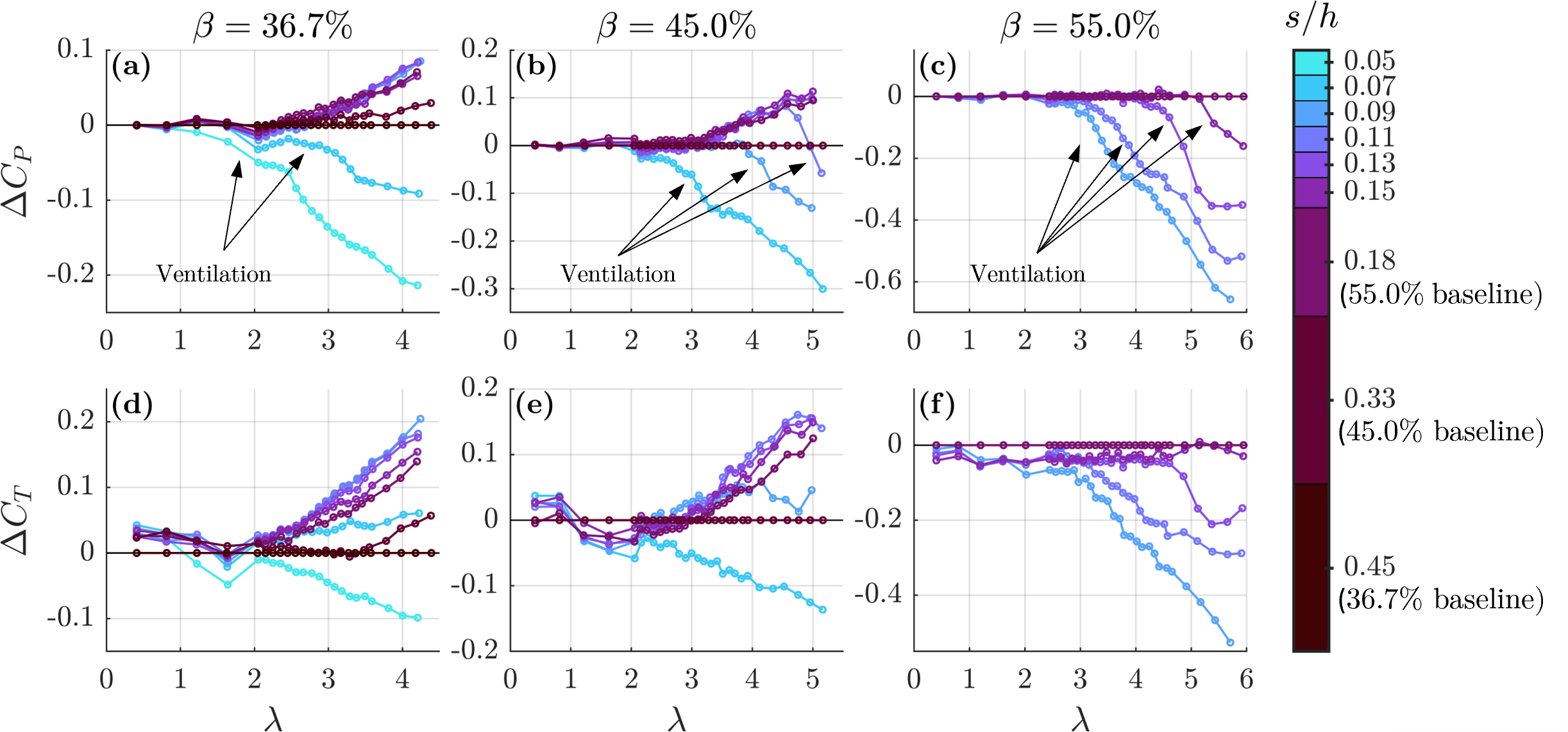
As mentioned in Section 2.2, $s/h$ was maximized at each blockage to minimize the impact of ventilation on array performance, particularly at the highest blockage ratios. However, this resulted in variation of $s/h$ across the tested $\beta$ (table 1). To assess the sensitivity of array performance to submergence depth, the array was also tested at a range of $s/h$ at $\beta=36.7\%$, $45.0\%$, and $55.0\%$ through variation of the rotors’ vertical position in the water column. The ADV position was likewise adjusted such that $U_{\infty}$ was always sampled at the turbine midplane.

The difference between the $C_{P}\!-\!\lambda$ and $C_{T}\!-\!\lambda$ curves presented in figure 6 and those obtained at different $s/h$ are shown in figure 21. At $\beta=36.7\%$ and $\beta=45.0\%$, both $C_{P}$ and $C_{T}$ increase slightly as $s/h$ decreases (i.e., the turbines are moved closer to the free surface), particularly for $\lambda$ beyond the performance peak. However, at all $\beta$, once $s/h$ drops below a critical value, ventilation begins, resulting in decreased $C_{P}$ and $C_{T}$ relative to deeper submergence depths. As $\beta$ increases, the onset of ventilation occurs at larger $s/h$ (i.e., deeper submergence), and at a given $\beta$, as $s/h$ decreases, ventilation begins at lower $\lambda$. However, other than ventilation, the effects of submergence depth on both $C_{P}$ and $C_{T}$ are minor relative to the influence of $\beta$ and the associated effects are mainly limited to $\lambda$ beyond the performance peak. Consequently, variation in $s/h$ across the tested $\beta$ is unlikely to significantly affect the trends presented in figure 6 or the flow field structure.

Figure 22: Change in the time-averaged normalized streamwise water depth profiles as a function of $s/h$ at 10 $\beta=36.7\%$, $\beta=45.0\%$, and 10 $\beta=55.0\%$ for 22–22 $\lambda=1.6$, 22–22 $\lambda=2.6$, and 22–22 $\lambda=3.6$. The farthest upstream measurement is taken at the center of the channel, whereas depth measurements in the vicinity of the array are directly upstream and downstream of Turbine B (Figure 3). For each case, depth measurements at each streamwise location ($h_{x}$) are normalized by the far-upstream water depth ($h$). The dashed lines indicate the swept area of Turbine B. The value of $s/h$ for each $\beta$ that corresponds to baseline experimental results (figure 10) is indicated in the colorbar and corresponds to the zero line in each tile.

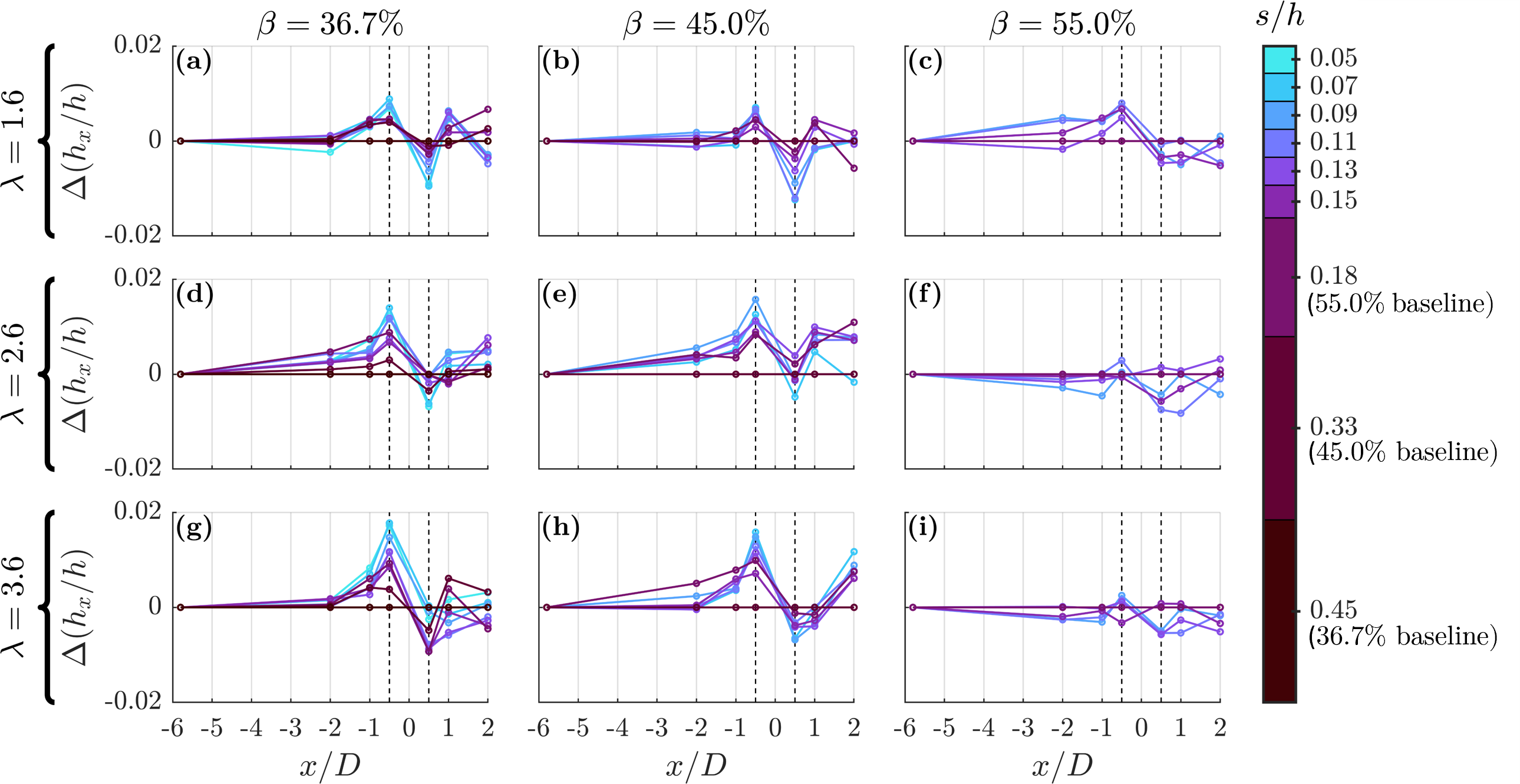
The normalized submergence depth also slightly affects free surface deformation in the vicinity of the array, as shown by the change in the water depth profiles in Figure 22 for $\lambda=1.6$, $2.6$, and $3.6$ at $\beta=36.7\%$, $45.0\%$, and $55.0\%$. Particularly for $\beta=36.7\%$ and $45.0\%$, decreasing $s/h$ somewhat elevates the free surface upstream of Turbine B and lowers the free surface directly downstream at $x/D=0.5$. In other words, the magnitude of the free surface drop across Turbine B somewhat increases with greater proximity of the rotor to the free surface, and this drop becomes more pronounced as $\lambda$ and $\beta$ increase. This is consistent with the non-ventilated power and thrust trends shown in figure 21. Trends in free surface deformation with $s/h$ at $\beta=55.0\%$ are less clear, likely due to the significant ventilation that occurs this blockage ratio. Similarly, for all cases trends in the free surface with $s/h$ further downstream ($x/D=1-2$) are more ambiguous, and may be obscured by the relatively low spatial and temporal resolution of the free surface transducers utilized in this study.

As noted in Section 2.3, the net lateral force on the array of two identical counter-rotating turbines is approximately zero when $\Delta\theta=0^{\circ}$ since the array is symmetric about its centerline. However, by defining the directions of positive $L_{A}$ and $L_{B}$ with this counter-rotation in mind as in figure 3, the array-average lateral force coefficient is nonzero and represents the average lateral force coefficient experienced by an individual rotor in the array as

$$C_{L,\mathrm{rotor}}=\frac{L_{A}+L_{B}}{\frac{1}{2}\rho U_{\infty}^{2}A_{\mathrm{turbines}}}\ \ .$$ (S.1)

Figure S.1: Time-averaged rotor-average lateral force coefficient as a function of $\beta$ and $\lambda$. The shaded regions indicate the interquartile range of the array- and cycle-averaged performance at each $\beta$ and $\lambda$ (the vertical span of the shaded region at each point is similar to the size of the markers for most operating conditions).

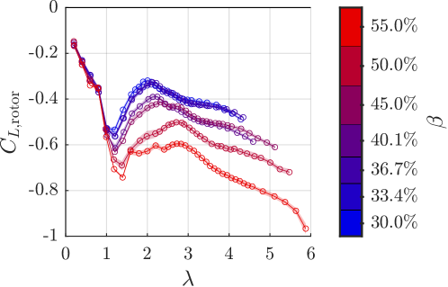
Figure S.1 shows the effect of blockage on $C_{L,\mathrm{rotor}}-\lambda$ curves across the tested $\beta$ and $\lambda$. As for $C_{P}$ and $C_{T}$, the magnitude of $C_{L,\mathrm{rotor}}$ at a particular $\lambda$ tends to increase with the blockage ratio. Additionally in a similar manner to the array power and thrust coefficients, $C_{L,\mathrm{rotor}}$ also exhibits invariance to $\beta$ at lower tip-speed ratios ($\lambda\leq 1$).

As noted in Section 3, the conventional definition of the array power coefficient (Eq. 6) neglects the potential energy that may be harnessed by the array in a confined flow. Consequently, at higher blockage, array efficiency may be better described using a hydraulic efficiency ($\eta$) that considers both the static and dynamic head in the flow:

$$\eta=\frac{Q_{A}\omega_{A}+Q_{B}\omega_{B}}{\dot{m}g\Delta h}\ \ ,$$ (S.2)

where $\dot{m}$ is the mass flow rate through the channel and $\Delta h$ is the difference in the water depth between far upstream and far downstream. Similar definitions of efficiency were employed by Takamatsu et al. (1985) and McAdam et al. (2013a) in their studies of high-blockage cross-flow turbines. However, both $\dot{m}$ and $\Delta h$ can be difficult to measure in practice. In this study, instrumentation to measure the volumetric flow rate through the flume was unavailable, and the volumetric flow rate is expected to vary with $\lambda$ at each $\beta$ due to interactions between the array and the channel (Hunt & Polagye, 2023). Additionally, accurate measurements of $\Delta h$ require a channel of sufficient length to allow the flow to fully mix downstream of the array and sufficient measurement resolution to identify this condition. For the experimental set-up in this study, the finite length of the flume downstream of the cross-flow turbine array is likely insufficient to allow the flow to fully mix, and the furthest downstream measurement of the water depth was taken only $2D$ downstream of the array.

Figure S.2: S.2 Time-average hydraulic efficiency estimated for the array, compared to S.2 the time-average array-average $C_{P}$ (reproduced from figure 6). The axes limits in figure S.2 are cropped to focus on non-spurious values of $\eta$.

Although precise measurements of $\dot{m}$ and $\Delta h$ are not available in this study, we present a rough estimate of $\eta$ for the experimental array across the tested range of $\beta$ and $\lambda$ using the available velocity and depth measurements. Assuming a uniform velocity profile in the Tyler flume, we estimate $\dot{m}\approx\rho U_{\infty}hw$. $\Delta h$ is estimated as the difference between the furthest upstream measured water depth (at $x/D=-5.8$) and furthest downstream measured water depth (at $x/D=2$). The resulting hydraulic efficiencies are expressed as a function of $\beta$ and $\lambda$ in figure S.2. Unlike $C_{P}$, the values of $\eta$ are $\leq 1$, with the exception of several spikes in the estimated $\eta$ at lower $\lambda$. These spikes occur when $\Delta h\approx 0$ between the two sample locations resulting from an irregular and unsteady free surface, and emphasizes the spatial and temporal resolution required to characterize the free surface deformation for the purposes of computing hydraulic efficiency. As $\lambda$ increases, the thrust on the array results in a more defined free surface profile and less noise in the estimates of hydraulic efficiency, with trends in $\eta$ with blockage largely following those of $C_{P}$ (figure S.2). Nonetheless, the $\eta$ shown are likely lower than the true hydraulic efficiencies, due to overestimation of the mass flow rate and total head drop from the available velocity and depth measurements.

Figure S.3: Time-averaged streamwise velocity $0.6D$ downstream of the array as function of $\beta$ and $\lambda$, normalized by the corresponding LMADT-modeled bypass velocity, $u_{b}$. The black rectangles in each tile indicate the projected area of the turbines in the field of view. Tiles corresponding to the optimal $\lambda$ for each blockage are outlined in purple (tiles (d), (h), and (k)), and correspond to figures 13, 13 and 13.

Figure S.4: Time-averaged streamwise velocity $0.6D$ downstream of the array as function of $\beta$ and $\lambda$, normalized by the corresponding LMADT-modeled wake velocity, $u_{w}$. The black rectangles in each tile indicate the projected area of the turbines in the field of view. Flow fields corresponding to the optimal $\lambda$ for each blockage are outlined in purple (tiles (d), (h), and (k)), and correspond to figures 13, 13 and 13.

Figure S.5: Time-averaged streamwise velocity $1.5D$ downstream of the array as function of $\beta$ and $\lambda$. Velocity measurements are normalized by the freestream velocity measured by the ADV. The black rectangles in each tile indicate the projected area of the turbines in the field of view. Flow fields corresponding to the optimal $\lambda$ for each blockage are outlined in purple (tiles (d), (h), and (k)).

Figure S.6: Time-averaged streamwise velocity $1.5D$ downstream of the array as function of $\beta$ and $\lambda$, normalized by the corresponding LMADT-modeled bypass velocity, $u_{b}$. The black rectangles in each tile indicate the projected area of the turbines in the field of view. Tiles corresponding to the optimal $\lambda$ for each blockage are outlined in purple (tiles (d), (h), and (k)).

Figure S.7: Time-averaged streamwise velocity $0.6D$ downstream of the array as function of $\beta$ and $\lambda$, normalized by the corresponding LMADT-modeled wake velocity, $u_{w}$. The black rectangles in each tile indicate the projected area of the turbines in the field of view. Flow fields corresponding to the optimal $\lambda$ for each blockage are outlined in purple (tiles (d), (h), and (k)).

Figure S.8: Conditions under which physically meaningful predictions for performance at $\beta_{2}$ can be obtained from the bluff-body forecasting method described in Section 5 and the collected performance data (figure 6), assuming constant $Fr_{h}$ between $\beta_{1}$ and $\beta_{2}$. The white regions in each panel represent combinations of $C_{T,1}$ and $\beta_{2}$ that yield physical, sub-critical solutions, whereas the black regions indicate combinations that yield non-physical solutions. The grey regions in each panel indicate $C_{T,1}$ outside of the range of values measured at each $\beta_{1}$, and the dashed blue line in each panel indicates $\beta_{1}$ relative to the range of $\beta_{2}$ that can be forecasted.

References

- Abutunis & Menta (2022) Abutunis, Abdulaziz & Menta, Venkata Gireesh 2022 Comprehensive Parametric Study of Blockage Effect on the Performance of Horizontal Axis Hydrokinetic Turbines. Energies 15 (7), 2585.
- Alexander & Holownia (1978) Alexander, A. J. & Holownia, B. P. 1978 Wind tunnel tests on a savonius rotor. Journal of Wind Engineering and Industrial Aerodynamics 3 (4), 343–351.
- Araya et al. (2017) Araya, Daniel B., Colonius, Tim & Dabiri, John O. 2017 Transition to bluff-body dynamics in the wake of vertical-axis wind turbines. Journal of Fluid Mechanics 813, 346–381.
- Araya & Dabiri (2015) Araya, Daniel B. & Dabiri, John O. 2015 A comparison of wake measurements in motor-driven and flow-driven turbine experiments. Experiments in Fluids 56 (7), 150.
- Bachant & Wosnik (2015) Bachant, Peter & Wosnik, Martin 2015 Characterising the near-wake of a cross-flow turbine. Journal of Turbulence 16 (4), 392–410.
- Bachant & Wosnik (2016) Bachant, Peter & Wosnik, Martin 2016 Effects of Reynolds Number on the Energy Conversion and Near-Wake Dynamics of a High Solidity Vertical-Axis Cross-Flow Turbine. Energies 9 (2), 73–73.
- Badshah et al. (2019) Badshah, Mujahid, VanZwieten, James, Badshah, Saeed & Jan, Sakhi 2019 CFD study of blockage ratio and boundary proximity effects on the performance of a tidal turbine. IET Renewable Power Generation 13 (5), 744–749.
- Bahaj et al. (2007) Bahaj, A. S., Molland, A. F., Chaplin, J. R. & Batten, W. M. J. 2007 Power and thrust measurements of marine current turbines under various hydrodynamic flow conditions in a cavitation tunnel and a towing tank. Renewable Energy 32 (3), 407–426.
- Barnsley & Wellicome (1990) Barnsley, M. J. & Wellicome, J. F. 1990 Final report on the 2nd phase of development and testing of a horizontal axis wind turbine test rig for the investigation of stall regulation aerodynamics. Technical Report E.5A/CON5103/ 1746. ETSU.
- Battisti et al. (2011) Battisti, L., Zanne, L., Dell’Anna, S., Dossena, V., Persico, G. & Paradiso, B. 2011 Aerodynamic Measurements on a Vertical Axis Wind Turbine in a Large Scale Wind Tunnel. Journal of Energy Resources Technology 133 (3).
- Birjandi et al. (2013) Birjandi, Amir Hossein, Bibeau, Eric Louis, Chatoorgoon, Vijay & Kumar, Anurag 2013 Power measurement of hydrokinetic turbines with free-surface and blockage effect. Ocean Engineering 69, 9–17.
- Chamorro et al. (2012) Chamorro, Leonardo P., Arndt, R.e.a & Sotiropoulos, F. 2012 Reynolds number dependence of turbulence statistics in the wake of wind turbines. Wind Energy 15 (5), 733–742.
- Chen & Liou (2011) Chen, T. Y. & Liou, L. R. 2011 Blockage corrections in wind tunnel tests of small horizontal-axis wind turbines. Experimental Thermal and Fluid Science 35 (3), 565–569.
- Consul et al. (2013) Consul, Claudio A., Willden, Richard H.J. & McIntosh, Simon C. 2013 Blockage effects on the hydrodynamic performance of a marine cross-flow turbine. Philosophical Transactions of the Royal Society A: Mathematical, Physical and Engineering Sciences 371 (1985), 20120299–20120299.
- Dehtyriov et al. (2021) Dehtyriov, D., Schnabl, A. M., Vogel, C. R., Draper, S., Adcock, T. a. A. & Willden, R. H. J. 2021 Fractal-like actuator disc theory for optimal energy extraction. Journal of Fluid Mechanics 927, A40.
- Dehtyriov et al. (2023) Dehtyriov, Daniel, Vogel, Christopher & Willden, Richard 2023 A Two-scale blockage correction for an array of tidal turbines. Proceedings of the European Wave and Tidal Energy Conference 15.
- Dossena et al. (2015) Dossena, Vincenzo, Persico, Giacomo, Paradiso, Berardo, Battisti, Lorenzo, Dell’Anna, Sergio, Brighenti, Alessandra & Benini, Enrico 2015 An Experimental Study of the Aerodynamics and Performance of a Vertical Axis Wind Turbine in a Confined and Unconfined Environment. Journal of Energy Resources Technology 137 (5).
- Garrett & Cummins (2007) Garrett, Chris & Cummins, Patrick 2007 The efficiency of a turbine in a tidal channel. Journal of Fluid Mechanics 588, 243–251.
- Gaurier et al. (2015) Gaurier, B., Germain, G., Facq, J. V., Johnstone, C. M., Grant, A. D., Day, A. H., Nixon, E., Di Felice, F. & Costanzo, M. 2015 Tidal energy “Round Robin” tests comparisons between towing tank and circulating tank results. International Journal of Marine Energy 12, 87–109.
- Gauthier et al. (2016) Gauthier, Etienne, Kinsey, Thomas & Dumas, Guy 2016 Impact of Blockage on the Hydrodynamic Performance of Oscillating-Foils Hydrokinetic Turbines. Journal of Fluids Engineering 138 (091103).
- Gauvin-Tremblay & Dumas (2020) Gauvin-Tremblay, Olivier & Dumas, Guy 2020 Two-way interaction between river and deployed cross-flow hydrokinetic turbines. Journal of Renewable and Sustainable Energy 12 (3), 034501–034501.
- Gauvin-Tremblay & Dumas (2022) Gauvin-Tremblay, Olivier & Dumas, Guy 2022 Hydrokinetic turbine array analysis and optimization integrating blockage effects and turbine-wake interactions. Renewable Energy 181, 851–869.
- Glauert (1935) Glauert, H. 1935 Airplane Propellers. In Aerodynamic Theory: A General Review of Progress Under a Grant of the Guggenheim Fund for the Promotion of Aeronautics (ed. William Frederick Durand), pp. 169–360. Berlin, Heidelberg: Springer.
- Goring & Nikora (2002) Goring, Derek G. & Nikora, Vladimir I. 2002 Despiking Acoustic Doppler Velocimeter Data. Journal of Hydraulic Engineering 128 (1), 117–126.
- Goude & Ågren (2014) Goude, Anders & Ågren, Olov 2014 Simulations of a vertical axis turbine in a channel. Renewable Energy 63, 477–485.
- Houlsby et al. (2008) Houlsby, G., Draper, S. & Oldfield, M. 2008 Application of linear momentum actuator disc theory to open channel flow. Technical Report OUEL 2296/08. University of Oxford.
- Houlsby & Vogel (2017) Houlsby, Guy & Vogel, Christopher 2017 The power available to tidal turbines in an open channel flow. Proceedings of Institution of Civil Engineers: Energy 170 (1), 12–21.
- Hunt & Polagye (2023) Hunt, Aidan & Polagye, Brian 2023 Experimental techniques for evaluating the performance of high-blockage cross-flow turbine arrays. In Proceedings of the 15th European Wave and Tidal Energy Conference, , vol. 15.
- Hunt et al. (2020) Hunt, Aidan, Stringer, Carl & Polagye, Brian 2020 Effect of aspect ratio on cross-flow turbine performance. Journal of Renewable and Sustainable Energy 12 (054501).
- Hunt et al. (2024) Hunt, Aidan, Strom, Benjamin, Talpey, Gregory, Ross, Hannah, Scherl, Isabel, Brunton, Steven, Wosnik, Martin & Polagye, Brian 2024 An experimental evaluation of the interplay between geometry and scale on cross-flow turbine performance. Renewable and Sustainable Energy Reviews 206, 114848.
- Jeong et al. (2018) Jeong, Houigab, Lee, Seungho & Kwon, Soon-Duck 2018 Blockage corrections for wind tunnel tests conducted on a Darrieus wind turbine. Journal of Wind Engineering and Industrial Aerodynamics 179, 229–239.
- Kinsey & Dumas (2017) Kinsey, Thomas & Dumas, Guy 2017 Impact of channel blockage on the performance of axial and cross-flow hydrokinetic turbines. Renewable Energy 103, 239–254.
- Kolekar & Banerjee (2015) Kolekar, Nitin & Banerjee, Arindam 2015 Performance characterization and placement of a marine hydrokinetic turbine in a tidal channel under boundary proximity and blockage effects. Applied Energy 148, 121–133.
- Kolekar et al. (2019) Kolekar, Nitin, Vinod, Ashwin & Banerjee, Arindam 2019 On Blockage Effects for a Tidal Turbine in Free Surface Proximity. Energies 12 (17), 3325.
- Maskell (1963) Maskell, E.C. 1963 A Theory of the Blockage Effects on Bluff Bodies and Stalled Wings in a Closed Wind Tunnel. Reports and Memoranda 3400. Ministry of Aviation.
- McAdam et al. (2013a) McAdam, R. A., Houlsby, G. T. & Oldfield, M. L. G. 2013a Experimental measurements of the hydrodynamic performance and structural loading of the Transverse Horizontal Axis Water Turbine: Part 1. Renewable Energy 59, 105–114.
- McAdam et al. (2013b) McAdam, R. A., Houlsby, G. T. & Oldfield, M. L. G. 2013b Experimental measurements of the hydrodynamic performance and structural loading of the transverse horizontal axis water turbine: Part 2. Renewable Energy 59, 141–149.
- McTavish et al. (2014) McTavish, S., Feszty, D. & Nitzsche, F. 2014 An experimental and computational assessment of blockage effects on wind turbine wake development. Wind Energy 17 (10), 1515–1529.
- Medici & Alfredsson (2006) Medici, D. & Alfredsson, P. H. 2006 Measurements on a wind turbine wake: 3D effects and bluff body vortex shedding. Wind Energy 9 (3), 219–236.
- Miller et al. (2018) Miller, Mark A., Duvvuri, Subrahmanyam, Brownstein, Ian, Lee, Marcus, Dabiri, John O. & Hultmark, Marcus 2018 Vertical-Axis Wind Turbine Experiments at Full Dynamic Similarity. Journal of Fluid Mechanics 844, 707–720.
- Miller et al. (2021) Miller, Mark A., Duvvuri, Subrahmanyam & Hultmark, Marcus 2021 Solidity effects on the performance of vertical-axis wind turbines. Flow 1.
- Nishino & Willden (2012a) Nishino, Takafumi & Willden, Richard H. J. 2012a Effects of 3-D channel blockage and turbulent wake mixing on the limit of power extraction by tidal turbines. International Journal of Heat and Fluid Flow 37, 123–135.
- Nishino & Willden (2012b) Nishino, Takafumi & Willden, Richard H. J. 2012b The efficiency of an array of tidal turbines partially blocking a wide channel. Journal of Fluid Mechanics 708, 596–606.
- Nishino & Willden (2013) Nishino, Takafumi & Willden, Richard H. J. 2013 Two-scale dynamics of flow past a partial cross-stream array of tidal turbines. Journal of Fluid Mechanics 730, 220–244.
- Pao & Johnson (2009) Pao, Lucy Y. & Johnson, Kathryn E. 2009 A tutorial on the dynamics and control of wind turbines and wind farms. In 2009 American Control Conference, pp. 2076–2089.
- Polagye et al. (2019) Polagye, Brian, Strom, Ben, Ross, Hannah, Forbush, Dominic & Cavagnaro, Robert J. 2019 Comparison of cross-flow turbine performance under torque-regulated and speed-regulated control. Journal of Renewable and Sustainable Energy 11 (4), 044501–044501.
- Ross & Polagye (2020a) Ross, Hannah & Polagye, Brian 2020a An experimental assessment of analytical blockage corrections for turbines. Renewable Energy 152, 1328–1341.
- Ross & Polagye (2020b) Ross, Hannah & Polagye, Brian 2020b An experimental evaluation of blockage effects on the wake of a cross-flow current turbine. Journal of Ocean Engineering and Marine Energy 6 (3), 263–275.
- Ross & Polagye (2022) Ross, Hannah & Polagye, Brian 2022 Effects of dimensionless parameters on the performance of a cross-flow current turbine. Journal of Fluids and Structures 114, 103726.
- Ross & Altman (2011) Ross, Ian & Altman, Aaron 2011 Wind tunnel blockage corrections: Review and application to Savonius vertical-axis wind turbines. Journal of Wind Engineering and Industrial Aerodynamics 99 (5), 523–538.
- Ryan et al. (2016) Ryan, Kevin J., Coletti, Filippo, Elkins, Christopher J., Dabiri, John O. & Eaton, John K. 2016 Three-dimensional flow field around and downstream of a subscale model rotating vertical axis wind turbine. Experiments in Fluids 57 (3), 1–15.
- Ryi et al. (2015) Ryi, Jaeha, Rhee, Wook, Chang Hwang, Ui & Choi, Jong-Soo 2015 Blockage effect correction for a scaled wind turbine rotor by using wind tunnel test data. Renewable Energy 79, 227–235.
- Sarlak et al. (2016) Sarlak, H., Nishino, T., Martínez-Tossas, L. A., Meneveau, C. & Sørensen, J. N. 2016 Assessment of blockage effects on the wake characteristics and power of wind turbines. Renewable Energy 93, 340–352.
- Scherl (2022) Scherl, Isabel 2022 Optimization, Modeling, and Control of Cross-Flow Turbine Arrays. PhD thesis, University of Washington, United States – Washington.
- Schluntz & Willden (2015) Schluntz, J. & Willden, R. H. J. 2015 The effect of blockage on tidal turbine rotor design and performance. Renewable Energy 81, 432–441.
- Steiros et al. (2022) Steiros, K., Bempedelis, N. & Cicolin, M. M. 2022 An analytical blockage correction model for high-solidity turbines. Journal of Fluid Mechanics 948, A57.
- Takamatsu et al. (1985) Takamatsu, Yasuo, Furukawa, Akinori, Okuma, Kusuo & Shimogawa, Yasuhiko 1985 Study on Hydrodynamic Performance of Darrieus-type Cross-flow Water Turbine. Bulletin of JSME 28 (240), 1119–1127.
- Vogel et al. (2016) Vogel, C. R., Houlsby, G. T. & Willden, R. H J 2016 Effect of free surface deformation on the extractable power of a finite width turbine array. Renewable Energy 88, 317–324.
- Westerweel & Scarano (2005) Westerweel, Jerry & Scarano, Fulvio 2005 Universal outlier detection for PIV data. Experiments in Fluids 39 (6), 1096–1100.
- Whelan et al. (2009) Whelan, J. I., Graham, J. M. R. & Peiró, J. 2009 A free-surface and blockage correction for tidal turbines. Journal of Fluid Mechanics 624, 281–291.
- Young et al. (2017) Young, Y. L., Harwood, C. M., Montero, F. Miguel, Ward, J. C. & Ceccio, S. L. 2017 Ventilation of Lifting Bodies: Review of the Physics and Discussion of Scaling Effects. Applied Mechanics Reviews 69 (1), 010801–010801.
- Zanforlin & Nishino (2016) Zanforlin, Stefania & Nishino, Takafumi 2016 Fluid dynamic mechanisms of enhanced power generation by closely spaced vertical axis wind turbines. Renewable Energy 99, 1213–1226.
- Zhang et al. (2023) Zhang, Dayu, Guo, Penghua, Cheng, Yixin, Hu, Qiao & Li, Jingyin 2023 Analysis of blockage correction methods for high-solidity hydrokinetic turbines: Experimental and numerical investigations. Ocean Engineering 283, 115185.
- Zilic de Arcos et al. (2020) Zilic de Arcos, Federico, Tampier, Gonzalo & Vogel, Christopher R. 2020 Numerical analysis of blockage correction methods for tidal turbines. Journal of Ocean Engineering and Marine Energy 6 (2), 183–197.