RoboMNIST: A Multimodal Dataset for Multi-Robot Activity Recognition Using WiFi Sensing, Video, and Audio

Abstract

We introduce a novel dataset for multi-robot activity recognition (MRAR) using two robotic arms integrating WiFi channel state information (CSI), video, and audio data. This multimodal dataset utilizes signals of opportunity, leveraging existing WiFi infrastructure to provide detailed indoor environmental sensing without additional sensor deployment. Data were collected using two Franka Emika robotic arms, complemented by three cameras, three WiFi sniffers to collect CSI, and three microphones capturing distinct yet complementary audio data streams. The combination of CSI, visual, and auditory data can enhance robustness and accuracy in MRAR. This comprehensive dataset enables a holistic understanding of robotic environments, facilitating advanced autonomous operations that mimic human-like perception and interaction. By repurposing ubiquitous WiFi signals for environmental sensing, this dataset offers significant potential aiming to advance robotic perception and autonomous systems. It provides a valuable resource for developing sophisticated decision-making and adaptive capabilities in dynamic environments.

Background & Summary

Signals of opportunity refer to the use of pre-existing, non-dedicated signals in the environment for secondary purposes beyond their original intent. WiFi signals, for instance, are primarily used for communication, but can also provide valuable information about the environment through channel state information (CSI). This data captures intricate details about the propagation of WiFi signals, including reflections, scattering, and absorption caused by objects and activities in the environment. By repurposing these ubiquitous WiFi signals, we can achieve comprehensive indoor environmental sensing without the need for additional sensor infrastructure.

Combining WiFi CSI with video and audio data creates a powerful multimodal system that significantly enhances activity recognition capabilities. Video data provides rich visual information, capturing spatial and temporal changes in the environment. Audio data adds another layer of contextual information, identifying auditory cues that correlate with specific activities. Integrating these modalities with CSI data leads to a more holistic understanding of the environment, enabling more accurate and reliable multi-robot activity recognition (MRAR).

The use of signals of opportunity, such as WiFi CSI, offers several key advantages. Firstly, it leverages existing infrastructure, reducing the cost and complexity associated with deploying additional sensors. This makes it an economically viable option for large-scale implementations. Secondly, the multimodal nature of the sensing network enhances robustness by compensating for the limitations of individual sensors. For instance, in scenarios where visual data may be obscured or audio data may be noisy, the complementary information from CSI can help maintain accurate activity recognition.

In recent decades, the integration of robotics and automated systems into various sectors has markedly transformed human life and industrial processes [1]. The advent of multi-agent systems, where multiple robots collaborate, has subtly yet significantly enhanced task efficiency and adaptability [2, 3]. In healthcare, robots perform complex surgeries with unprecedented precision, reducing recovery times and improving outcomes. In manufacturing, automated assembly lines and robotic arms ensure consistent quality and high productivity, revolutionizing production techniques. Additionally, robots are deployed in hazardous environments, like disaster sites [4], minimizing human risks.

In the realm of robotics, the integration of multimodal learning systems represents a significant leap towards achieving autonomous operations that closely mimic human-like perception and interaction with the environment [5]. This paper explores the application of such an advanced learning paradigm through the deployment of two Franka Emika robotic arms, a choice inspired by their versatility and precision in complex tasks [6]. To enrich the sensory framework essential for multimodal learning, we employ a comprehensive array of sensors: three cameras, three WiFi sniffers, and three microphones. Each modality is strategically chosen to capture distinct yet complementary data streams—visual, wireless signal-based, and auditory—thereby enabling a more holistic understanding of the robotic arms’ surroundings and activities. This multi-sensory approach not only facilitates the robust perception required for intricate manipulations and interactions but also paves the way for groundbreaking advancements in autonomous robotic systems capable of sophisticated decision-making and adaptation in dynamic environments.

The MNIST dataset [7], featuring handwritten digits classified into ten categories, was first introduced by LeCun et al. in 1998. At that time, the significant advancements and performance of deep learning techniques were unimaginable. Despite the current extensive capabilities of deep learning, the simple MNIST dataset remains the most widely used benchmark in the field, even surpassing CIFAR-10 [8] and ImageNet [9] in popularity according to Google Trends. Its simplicity hasn’t diminished its usage, despite some in the deep learning community advocating for its decline [10].

In this paper, we introduce the RoboMNIST dataset, an innovative extension of the traditional MNIST dataset tailored for robotic applications. This dataset features two Franka Emika robots writing different digits on an imaginary plane within a 3D environment. Our sensor-rich modules, comprising CSI, video, and audio, capture comprehensive data from the environment. We have validated the dataset’s integrity across individual data modalities through a series of experiments.

Methods

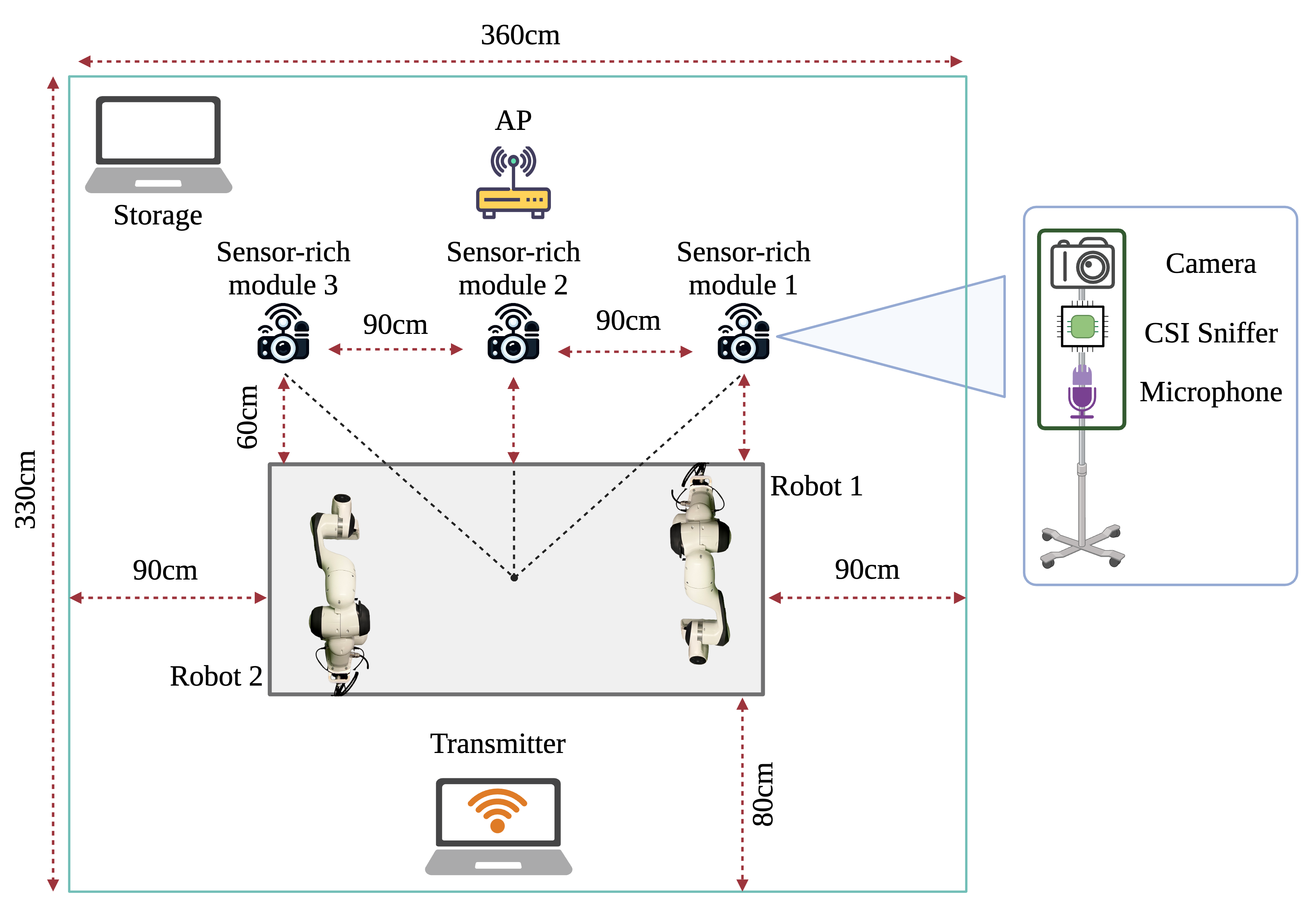
The data collection process was conducted in a laboratory, featuring desks, chairs, monitors, and various other office objects in the environment. The layout of the laboratory, along with its physical dimensions, is illustrated in Figure 1.

Figure 1: Floor plan of the data collection environment, where the robots are performing different activities while various sensors mounted on our sensor-rich modules capture data.

Hardware Specifications & Communication

In all the experiments we have used three sensor-rich modules that are positioned in the room capturing data while the two robotic arms are performing different activities. Each sensor-rich module is capable of simultaneously capturing three modalities namely CSI, video, and audio from the environment. Each module is equipped with the following hardware:

• CSI: A Raspberry Pi 4 Model B, integrated with the Nexmon project [11], which passively captures the CSI data.

• Video: A ZED 2 Stereo Camera for video recording.

• Audio: A CG CHANGEEK Mini USB Microphone, featuring omni-directional directivity, to record audio.

Figure 2 depicts the sensor-rich modules used in our data collection setup. We use $M\in\{1,2,3\}$ to denote the modules based on the numbering notation in Figure 1 in the rest of the paper. To facilitate the collection of CSI data, an Apple Mac Mini equipped with the 802.11ax WiFi 6 standard served as the WiFi transmitter.

Figure 2: Sensor-rich module used in the data collection setup consisting of a Raspberry Pi to capture CSI, a stereo camera to capture video, and a microphone to capture audio.

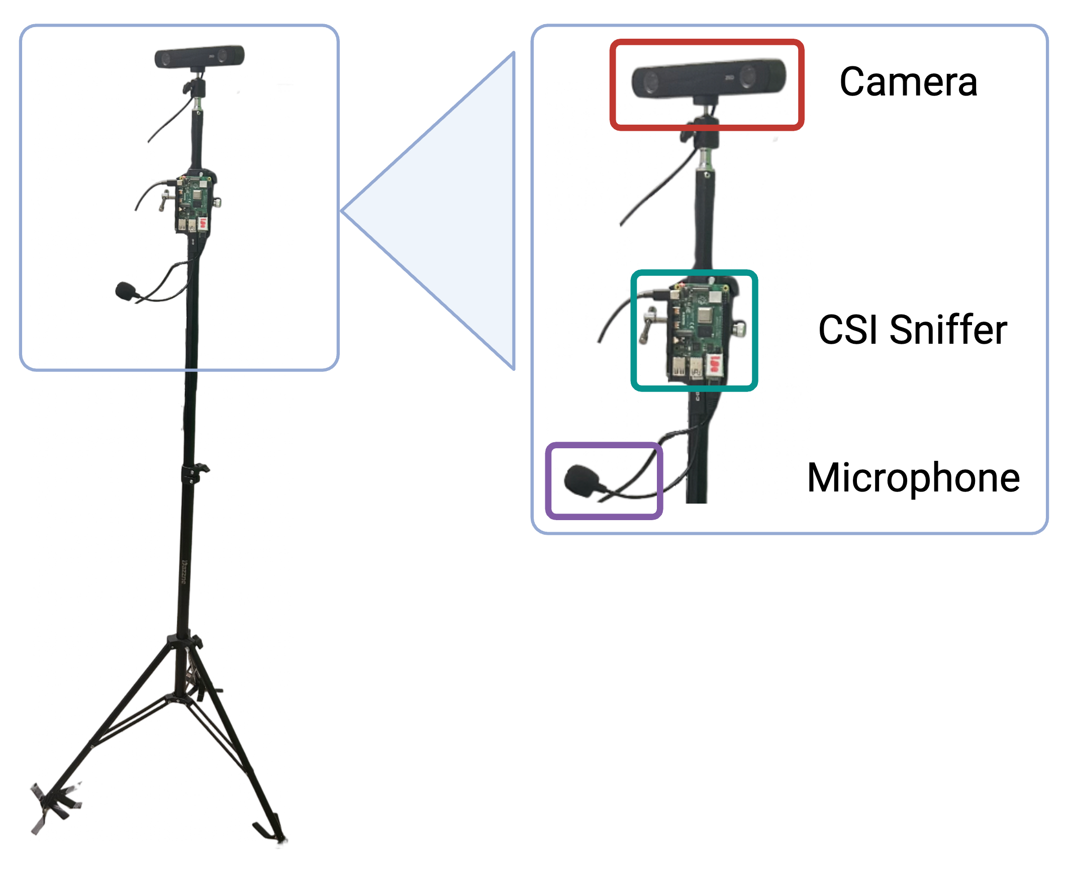
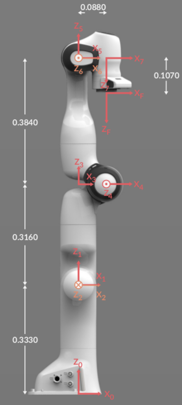
Figure 3 shows the Franka Emika Panda robot used in this dataset and its kinematic parameters according to the Denavit-Hartenberg convention. This robot is equipped with a $7$-axis revolute joint. The Franka Emika robotic arm is a collaborative robot (cobot) designed to work safely alongside humans in various environments, ranging from industrial settings to direct interaction scenarios. Unlike conventional industrial robots, which are typically enclosed for safety reasons, the Franka Emika arm can perform tasks in close proximity to people without posing a hazard [6]. This capability makes it ideal for operations that require direct physical interaction, such as drilling, screwing, polishing, and a wide range of inspection and assembly tasks. The Franka Emika robotic arm provides a $3$ kg payload capacity and a reach of $850$ mm. The robot weighs approximately $18$ kg and its repeatability is $0.1$ mm. Repeatability is a measure of the ability of the robot to consistently reach a specified point.

Frame	$a$ (m)	$d$ (m)	$\alpha$ (rad)	$\theta$ (rad)
Joint 1	0	0.333	0	$q_{1}$
Joint 2	0	0	$-\pi/2$	$q_{2}$
Joint 3	0	0.316	$\pi/2$	$q_{3}$
Joint 4	0.0825	0	$\pi/2$	$q_{4}$
Joint 5	-0.0825	0.384	$-\pi/2$	$q_{5}$
Joint 6	0	0	$\pi/2$	$q_{6}$
Joint 7	0.088	0	$\pi/2$	$q_{7}$
Flange	0	0.107	0	0
End effector (EE)	0	0.1034	0	$\pi/4$

Figure 3: Denavit-Hartenberg Parameters [12] and image [13] of Franka Emika robotic arm, with $q_{i}$ being the joint angle of the $i$th revolute joint.

Experiments

Our dataset is composed of $60$ different primary combinations performed by the robotic arms, capturing activities through our sensor-rich modules. Our dataset encompasses four variations:

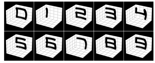
• Activity: The Franka Emika robotic arms were programmed to draw the numbers $0$ through $9$ on a vertical imaginary plane, resulting in ten distinct classes of activities. The end effector’s positions for each activity are illustrated in Figure 4. We denote the activities performed by the robots as $A\in\{0,1,\cdots,9\}$.

• Robot number: Indicated by $R\in\{1,2\}$, this specifies which of the two available robotic arms is performing the activity based on the numbering notation in Figure 1.

• Robot velocity: Denoted by $V\in\{\text{{High}},\>\text{{Medium}},\>\text{{Low}}\}$, this describes the velocity level at which the robot performs the activity.

• Motion uncertainty: Denoted by $U\in\mathbb{R}^{+}$, where $\mathbb{R}^{+}$ represents the positive real numbers, measures the $L_{2}$ norm error of the end effector’s position relative to its intended trajectory over time.

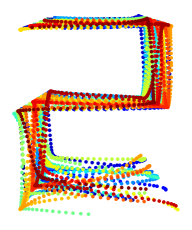
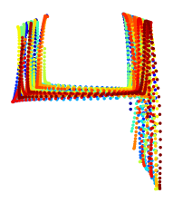
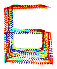
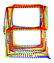
The combination of ten activities, two robots performing these activities, and three velocity levels results in a total of $60$ unique primary combinations. For each primary combination, we have collected $32$ repetitions. Each repetition spans $15$ seconds, during which the robot performs the action with consistent variations in activity, robot arm, and velocity, while incorporating motion uncertainty. This introduces deviations in each repetition as the robot writes on an imaginary plane, adding a realistic layer of complexity to the dataset. Figure 5 shows the uncertainty in motion of all the repetitions in four of the primary combinations as a sample projected on a 2D imaginary plane.

Figure 4: Numbers $0$ through $9$ are drawn by the robotic arm on a vertical imaginary plane, resulting in 10 distinct classes of activities. The plot shows the end effector trajectories that form these numbers, with the robotic arm and background removed for clarity. For illustration purposes the initial and final parts of the robot’s trajectory, where the robot positions itself from its starting point to the imaginary plane and back, are omitted.

(a) $A=2$

(b) $A=4$

(c) $A=6$

(d) $A=8$

Figure 5: Motion uncertainty of all the repetitions in four of the primary combinations as a sample. All with $R=1$, and $V=\text{{High}}$, but with different values of $A$. For illustration purposes, the path is projected on a 2D imaginary plane and the initial and final parts of the robot’s trajectory, where the robot positions itself from its starting point to the imaginary plane and back, are omitted.

WiFi CSI Modality

As wireless signals propagate, they encounter various obstacles in the environment, leading to reflections and scattering, a phenomenon known as multipath fading [14]. WiFi CSI facilitates the analysis of subcarrier propagation from the transmitter to the receiver in wireless communications [15]. The channel model is represented as

$$\mathbf{y}=\mathbf{Hx}+\boldsymbol{\eta},$$ (1)

where $\mathbf{x}$, $\mathbf{y}$, and $\boldsymbol{\eta}$ denote the transmitted signal vector, received signal vector, and additive noise vector, respectively [15]. The channel matrix $\mathbf{H}\in\mathbb{C}^{T\times S}$ encapsulates the characteristics of the wireless channel, including multipath propagation, fading, and other impairments, and is defined as

$$\mathbf{H}=\left[\begin{array}[]{cccc}h_{1}[1]&h_{2}[1]&\ldots&h_{S}[1]\\ h_{1}[2]&h_{2}[2]&\ldots&h_{S}[2]\\ \vdots&\vdots&\ddots&\vdots\\ h_{1}[T]&h_{2}[T]&\ldots&h_{S}[T]\end{array}\right],$$ (2)

where $S$ and $T$ represent the number of subcarriers for each antenna and the number of transmitted packets, respectively. Each element of the matrix $\mathbf{H}$ corresponds to a complex value, known as the channel frequency response, and is given by

$$h_{s}[t]=a_{s}e^{j\phi_{s}},$$ (3)

where $a_{s}$ and $\phi_{s}$ denote the amplitude and phase of subcarrier $s$ at timestamp $t$, respectively. For human activity recognition (HAR)[16, 17, 18] and robot activity recognition (RAR)[19, 20, 21], studies primarily focus on $\mathbf{A}\in\mathbb{R}^{T\times S}$, which corresponds to the element-wise amplitude of $\mathbf{H}$, disregarding the phase component.

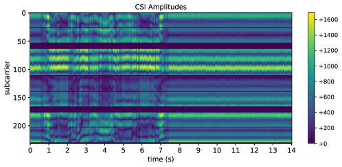
For each 15-second repetition, we collected CSI measurements at a $30$ Hz frequency, over an $80$ MHz bandwidth which gives $256$ number of subcarriers at each time stamp. This resulted in a $450\times 256$ complex matrix for each sensor-rich module. These matrices are stored in a json file. Additionally, we included received signal strength (RSS) information for each timestamp as well. Figure 6 displays a sample plot of the amplitudes of a CSI matrix.

Figure 6: Plot of CSI amplitudes, in a repetition with $A=0$, $R=1$, and $V=\text{{High}}$, while $M=1$ module capturing the CSI measurements.

Video Modality

For each 15-second repetition, we collected video measurements at a frequency of $30$ Hz, synchronized with the CSI measurements, using three sensor-rich modules, each containing a stereo camera. For each sample, three ZED 2 stereo cameras simultaneously recorded RGB videos at a resolution of $2560\times 720$ pixels, with the frames from the left and right lenses of each stereo camera horizontally concatenated. This setup allowed us to capture three different views of the same action. Each camera, equipped with two lenses, provided stereo video, resulting in a dataset that includes $3\text{ (cameras)}\times 2\text{ (lenses)}=6$ videos for each repetition.

Audio Modality

Audio signals are continuous waveforms that represent sound waves in a format that can be processed by digital systems. These waveforms are characterized by frequency, amplitude, and phase, which contain rich information about the environment and the sources of sound. In the context of activity recognition, audio signals offer a non-intrusive and cost-effective means to infer activities and interactions. By analyzing the acoustic patterns and variations over time, it is possible to identify specific activities based on the distinct sounds associated with each activity. Advanced machine learning algorithms, particularly those leveraging deep learning, have demonstrated significant success in classifying and recognizing activities from audio data. These algorithms extract useful information, such as the frequency and amplitude of the sound wave over time, to analyze and predict activities [22, 23].

In this paper, we employ auditory perception as many robot activities produce characteristic sounds from which we can effectively infer corresponding actions. We view audio not as a replacement but as a complement to existing sensory modalities. By fusing audio with other sensory data, we aim to achieve particularly robust activity recognition across a wide range of conditions. This multimodal approach enhances the accuracy and reliability of activity recognition systems, making them more effective in diverse environments.

Figure 7: Plot of audio spectrogram, in a repetition with $A=0$, $R=1$, and $V=\text{{High}}$, with $M=1$ module capturing the audio.

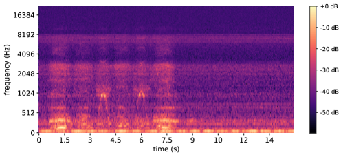
For each 15-second repetition, we collected audio measurements from each sensor-rich module at a sampling rate of $44{,}100$ Hz while the start and end times were synchronized with our other modalities. To analyze the audio data, we preprocess the audio files by computing their spectrograms. While we delve more into the calculation of the audio spectrogram in the Technical Validation section, a sample spectrogram plot of one of the captured audio is shown in Figure 7.

True Trajectory

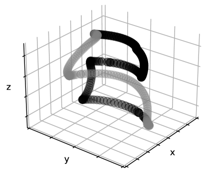
For each 15-second repetition, we provided the true joint positions of the robots at a frequency of $30$ Hz, synchronized with the CSI and video measurements. At each timestamp, each joint position, consisting of $q_{1}$ to $q_{7}$, corresponding to the $7$-axis revolute joints of the robot, has been stored in radians in a json file. For convenience, the $x-y-z$ position of the end effector (EE) in the Cartesian coordinate system is also provided. Figure 8 displays a sample plot of the end effector’s Cartesian position of one of the robots performing an activity.

Figure 8: Plot of the end effector’s position of the robot during a repetition with $A=2$, $R=1$, and $V=\text{{High}}$. The black trajectory represents the robot drawing the number on an imaginary plane, while the gray trajectory illustrates the robot’s movement from a fixed starting position to the imaginary plane and back.

Synchronization

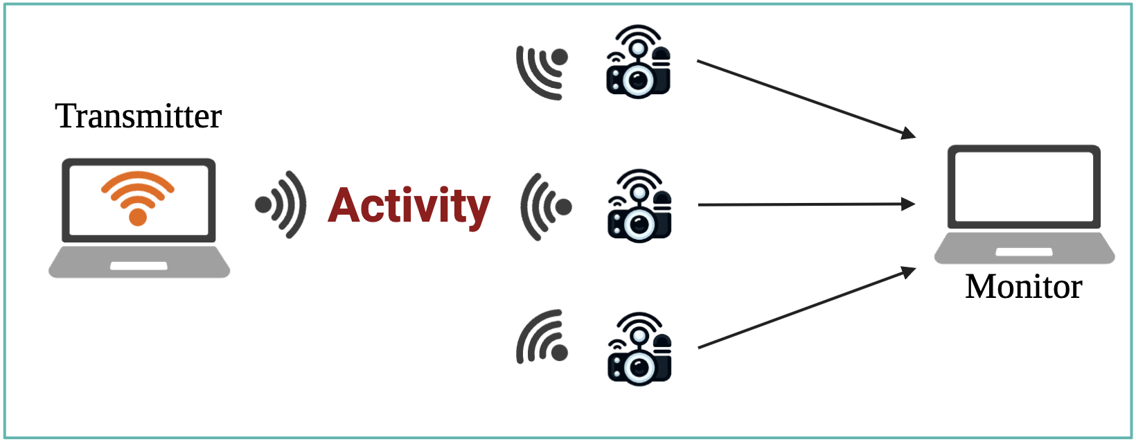
During data collection, each module incorporates local timestamping directly on the hardware. The timestamped data is subsequently transmitted across the network for further processing. Although this configuration effectively captures data from individual modules, synchronizing timestamps is critical for deployments involving multiple modules. To address this challenge, we developed a method whereby packets containing CSI, video, and audio data, each with its own timestamp, are redirected to a specialized system known as the monitor.

The monitor serves as a central hub, collecting packets from various modules and assigning synchronized timestamps to the data. A visual depiction of this intercommunication process is presented in Figure 9. Notably, according to the Nexmon project’s specifications, Raspberry Pis configured as CSI sniffers forfeit their WiFi communication capabilities. To overcome this restriction, we connected the sniffers and the monitor using Ethernet cables, thus ensuring uninterrupted communication between them.

Figure 9: Communication setup between modules and the monitor. The modules will gather the data and transfer them using a wire connection to the monitor for further processing, timestamping, and synchronization during the data collection procedure.

Using this configuration, the CSI, video, the true trajectories of the robots, and the start and end time of the audio are synchronized with each other and between all the sensor-rich modules, providing a comprehensive dataset for multi-modal passive MRAR. Figure 10 compactly shows different synchronized modalities in an experiment.

Figure 10: Plot of the three modalities and the robot’s true trajectory in a repetition with $A=0$, $R=1$, and $V=\text{{High}}$, captured by module $M=1$. The video, CSI, true trajectory, and start and end time of the audio are synchronized. For illustration purposes, the initial and final parts of the robot’s movement, where it positions itself from its starting point to the imaginary plane and back, are omitted.

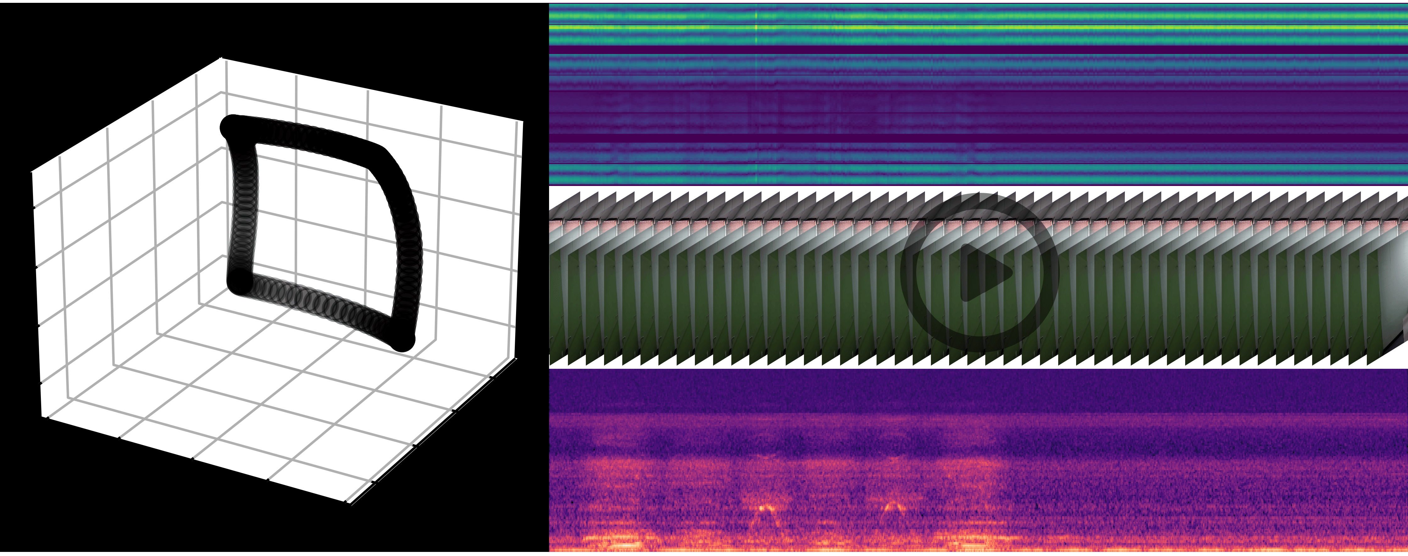
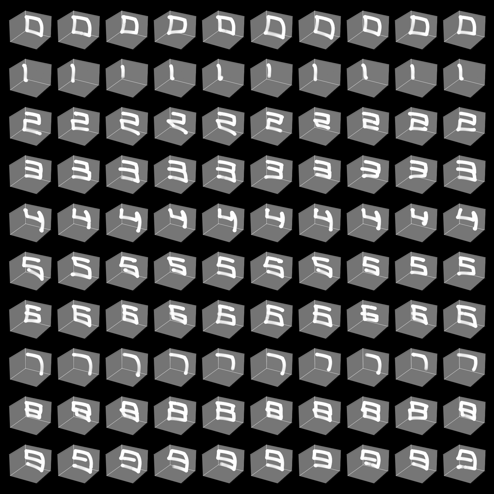
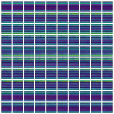
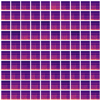
Figure 11 shows MNIST formatted plots of the $10$ activities and different repetitions based on our modalities.

(a) True Trajectory

(b) WiFi CSI Amplitude

(c) Video

(d) Audio Spectrogram

Figure 11: MNIST formatted plots of the true trajectory, WiFi CSI amplitude, video, and audio spectrogram. Each row represents activities from $0$ to $9$ and the columns are different repetitions in the same primary combination.

Data Records

The dataset is available for download from our Figshare repository [24].

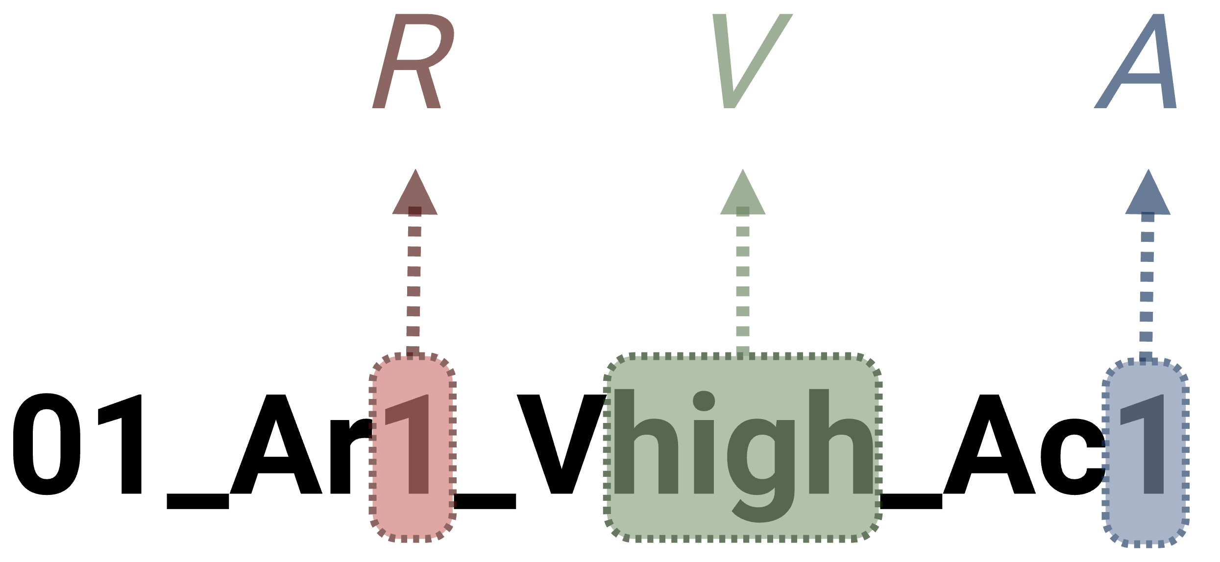
Based on variations in activity, robot, and velocity, we have $60$ primary combinations. Each combination has a dedicated folder in the dataset, named according to the standard described in Figure 12(a). Within each primary combination, there are at least $32$ repetitions, all with $15$-second duration and specific $R$, $V$, and $A$ variations, differing only by assigned motion uncertainty. Each repetition contains $8$ files as listed in Table 1, following the naming convention outlined in Figure 12(b).

(a) folders naming standard

(b) files naming standard

Figure 12: Naming standard for folders and files in our dataset. The naming standard for folders, dedicated to each primary combination, specifies the robot performing the activity (denoted by $R$), the velocity of the activity (denoted by $V$), and the specific activity being performed (denoted by $A$). The naming standard for each file within a folder shares the same values for $A$, $V$, and $R$, and varies by the robot’s motion uncertainty (denoted by $U$). The value of $U$ is always a floating-point number with two decimal places. For example, UNC258 represents $U=2.58$. The Rx indicates the module from which the data is sourced; it can be a specific number or "all," where "all" signifies that data from all sensors/robots are collected in the same file.

Data	Associated files
CSI	One json file containing CSI data for all modules
Video	Three mp4 files containing video data for each module
Audio	Three wav files containing audio data for each module
True robot trajectory	One json file containing trajectory data for both robots

Table 1: Associated files and their formats corresponding to each repetition of a primary combination.

WiFi CSI Description

This section describes the structure of the data files residing in the CSI files, which are the files ending with csi.json. Each repetition is represented by a single CSI file, which contains the CSI data for all the three sensor-rich modules. These CSI files are in json format and consist of an array of three json objects. Each json object corresponds to one of the sensor-rich modules. Within each json object, data is organized as a set of key-value pairs, as detailed in Table 2.

Key	Type	Value
module_number	Integer, either $1$, $2$, or $3$	The module number based on Figure 1
time_stamp_ns	Array of integer numbers	The timestamps of CSI collections in nanoseconds
complex_csi	Matrix of complex numbers	The CSI matrix as defined in eq. 2, where each row corresponds to a timestamp
RSS	Array of integer numbers	The RSS values at each timestamp

Table 2: Description of key-value sets of json objects in CSI files.

Video Description

This section describes the structure of the data files residing in the video files, identified by the cam.mp4 extension. Each repetition corresponds to $3$ video files, each for one of the sensor-rich modules. Each video file is in mp4 format, where each frame consists of the horizontally concatenated left and right frames of the lenses of the stereo camera, resulting in a final frame with dimensions of $2560\times 720$. Each frame is synchronized with the timestamps provided in the CSI file of the same repetition.

Audio Description

This section describes the structure of the data files residing in the audio files, identified by the mic.wav extension. Each repetition corresponds to three audio files, each file for one of the sensor-rich modules. Each audio file is in wav format and has been recorded for the $15$-second duration of the repetition.

True Robot Trajectory Description

This section describes the structure of the data files in the position files, which have the pos.json extension. Each repetition corresponds to one position file containing the position information of both robots. Even though only one robot is moving in each repetition, as indicated by the file name, we have included the position data for both robots. Each position file is in json format and consists of an array of two json objects, one for each robot. Each json object is a set of key-value pairs, as detailed in Table 3.

Key	Type	Value
robot_number	Integer, either $1$ or $2$	The robot number based on Figure 1
time_stamp_ns	Array of integer numbers	The timestamps of robot positions in nanoseconds (synchronized with CSI timestamps)
joint_positions	Matrix of floating point numbers	The joint positions of the robot in radian, where each row corresponds to a timestamp
EE_positions	Matrix of floating point numbers	The Cartesian positions of the robot’s end effector in meter, where each row corresponds to a timestamp

Table 3: Description of key-value sets of json objects in position files.

Technical Validation

WiFi CSI

Using the collected data from the three strategically located CSI sniffers mounted on our sensor-rich modules, we train two models: a vision transformer (ViT)[25] and a convolutional neural network (CNN) [26]. For both models, the amplitude of CSI from each sniffer is computed and then concatenated, to be fed to the models. The length of each sample is 15 seconds with $30$ Hz sampling frequency, which results in 450 timestamps, and also, the WiFi transmission bandwidth is $80$ MHz, which provides $256$ subcarriers at each timestamp, so each sample contains a complex CSI matrix $\mathbf{H}\in\mathbb{C}^{450\times 256}$, which after removing the pilot and unused subcarriers and computing the amplitude of CSI we have matrix $\mathbf{A}\in\mathbb{R}^{450\times 236}$ for each of the CSI sniffers.

Figure 13: Different steps of training our CNN model, from CSI collection to classification.

The proposed CNN model for action classification is structured to effectively capture and interpret spatial hierarchies in the input data, as shown in Figure 13. The architecture begins with two convolutional layers: the first layer employs 16 filters with a kernel size of $3\times 3$, stride of $1$, and padding of $1$, ensuring the preservation of spatial dimensions; the second layer follows a similar configuration but increases the filter count to $32$, allowing for deeper feature extraction. Each convolutional layer is followed by a rectified linear unit (ReLU) activation function to introduce non-linearity and a max-pooling operation with a kernel size of $2\times 2$ added after the first convolutional layer to down-sample the feature maps, reducing the dimensionality and computational load while retaining essential features. The dropout layer with a dropout rate of $0.5$ is included to prevent overfitting by randomly setting a fraction of the input units to zero during training. The flattened feature maps are then fed into a fully connected layer with $623{,}616$ units, producing output logits for $10$ classes corresponding to the activities performed by both robots. The training setup involves $80$ epochs with an early stopping patience of $10$, a batch size of $16$, a learning rate of $1\times 10^{-3}$, and a weight decay of $1\times 10^{-4}$ to mitigate overfitting by penalizing large weights. These parameters were chosen to balance the trade-offs between model complexity, training time, and generalization performance.

The other proposed method employs a ViT model to handle and classify CSIs based on their patches effectively. The custom dataset is designed to preprocess images by dividing them into smaller, non-overlapping patches, which facilitates the ViT’s ability to capture localized features and relationships within the CSI. Each CSI matrix is augmented by adding a channel dimension and then partitioned into patches of a specified size, enhancing the model’s ability to manage high-dimensional data efficiently.

Figure 14: Different steps of training ViT model, from CSI collection to classification.

The ViT model architecture includes several key components, as shown in Figure 14. First, an embedding layer flattens and projects the CSI patches into a high-dimensional space, transforming each patch into an input vector suitable for the transformer. The core of the model is a multi-layer transformer encoder, which consists of multiple transformer encoder layers. Each layer uses multi-head self-attention mechanisms to capture intricate relationships and dependencies between patches, followed by position-wise feed-forward networks to process these interactions. The output from the transformer encoder layers is then aggregated by averaging, ensuring that the global context of the image is considered. Finally, a fully connected layer maps the aggregated features to the desired number of classes, producing the classification logits. Dropout with a $0.45$ rate is applied to the fully connected layer to mitigate overfitting and improve the model’s generalization performance.

The training configuration is meticulously chosen to balance model complexity and performance, by applying grid search. The patch size is set to 116, enabling the model to handle substantial spatial information within each patch. The batch size of $32$ and $150$ training epochs ensure a robust training process, while the learning rate of $5\times 10^{-5}$ and weight decay of $1\times 10^{-6}$ are selected to optimize convergence and prevent overfitting. The ViT model utilizes $4$ attention heads and $7$ transformer layers, with a dropout rate of $0.3$ to maintain regularization and model stability. These design choices collectively enhance the model’s capacity to classify CSIs accurately across $10$ different activity classes.

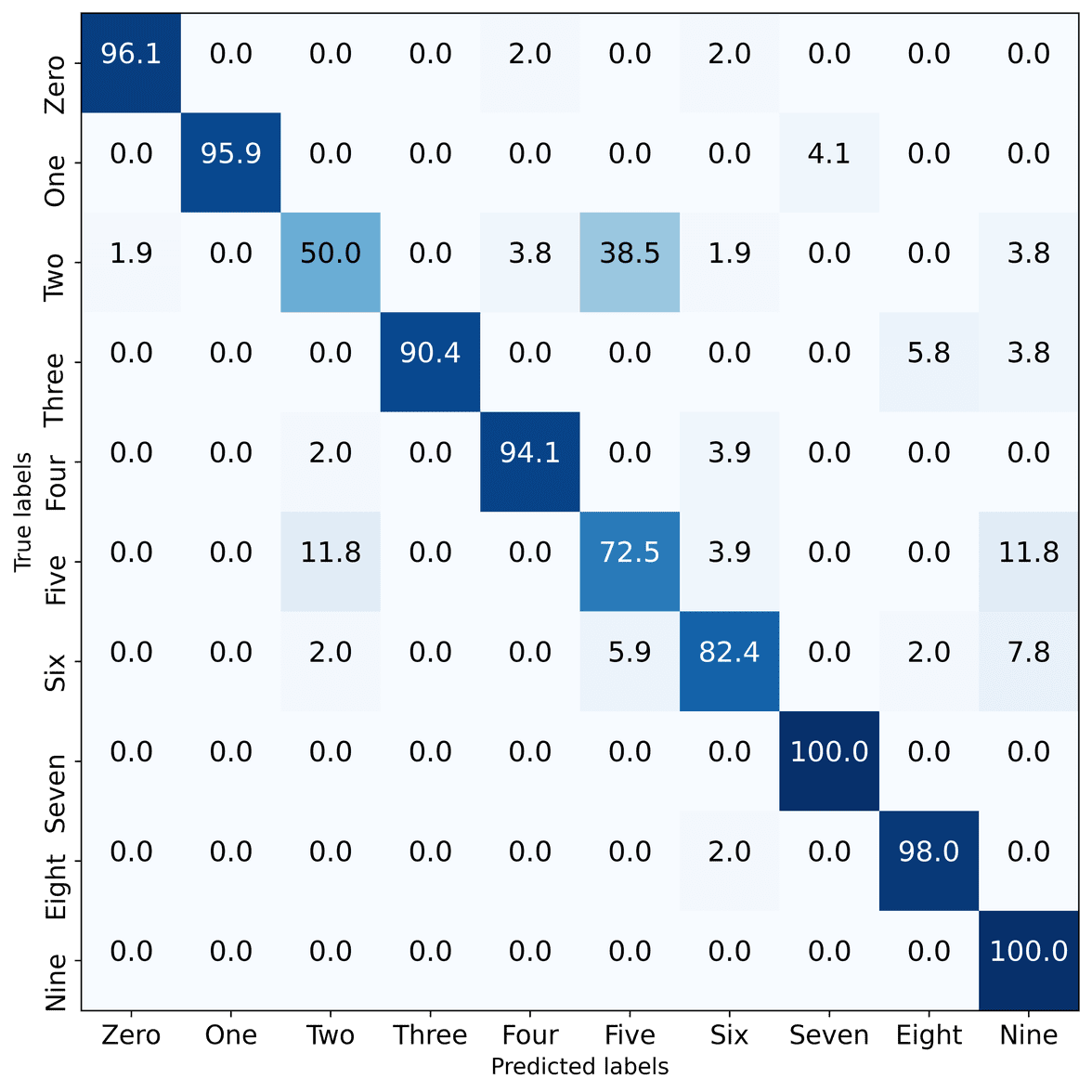
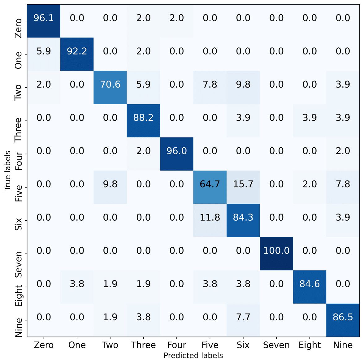
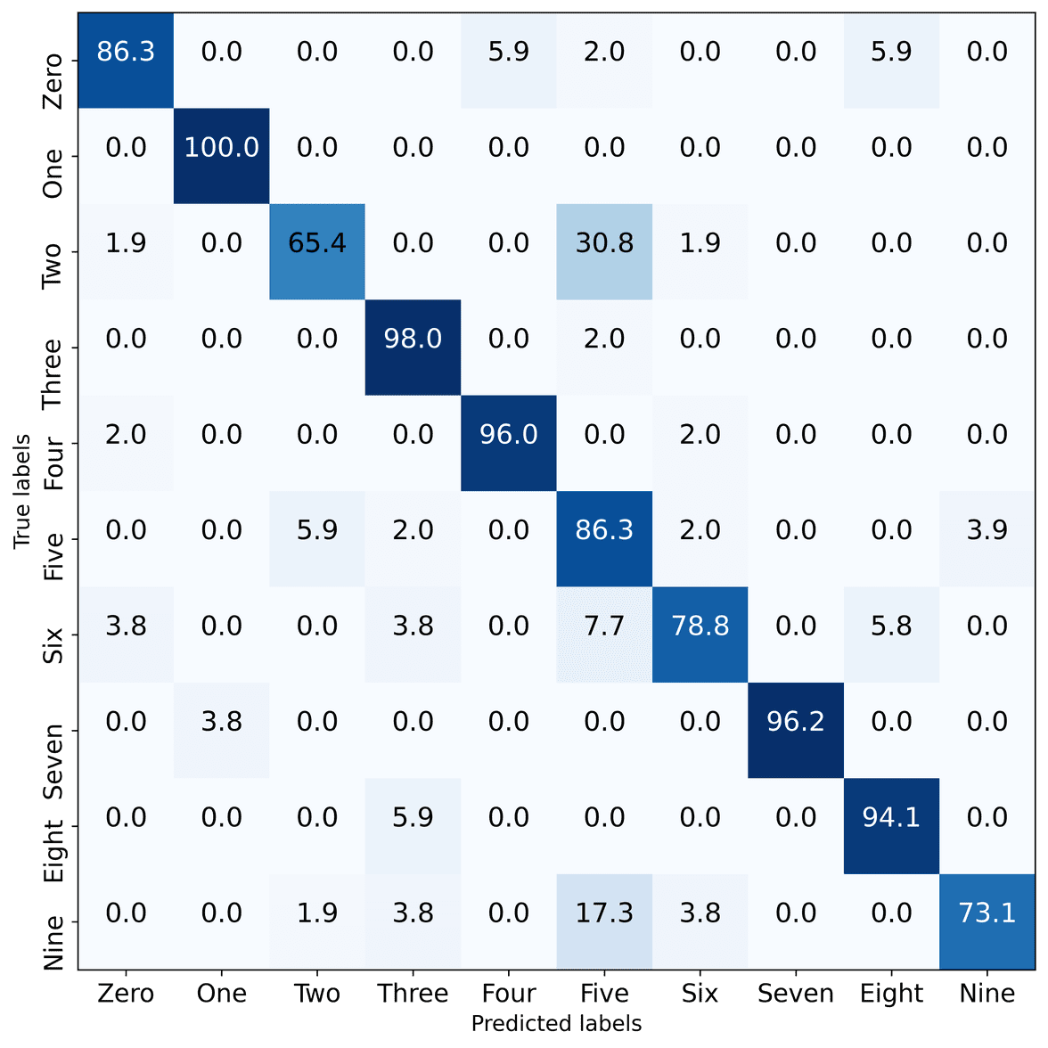
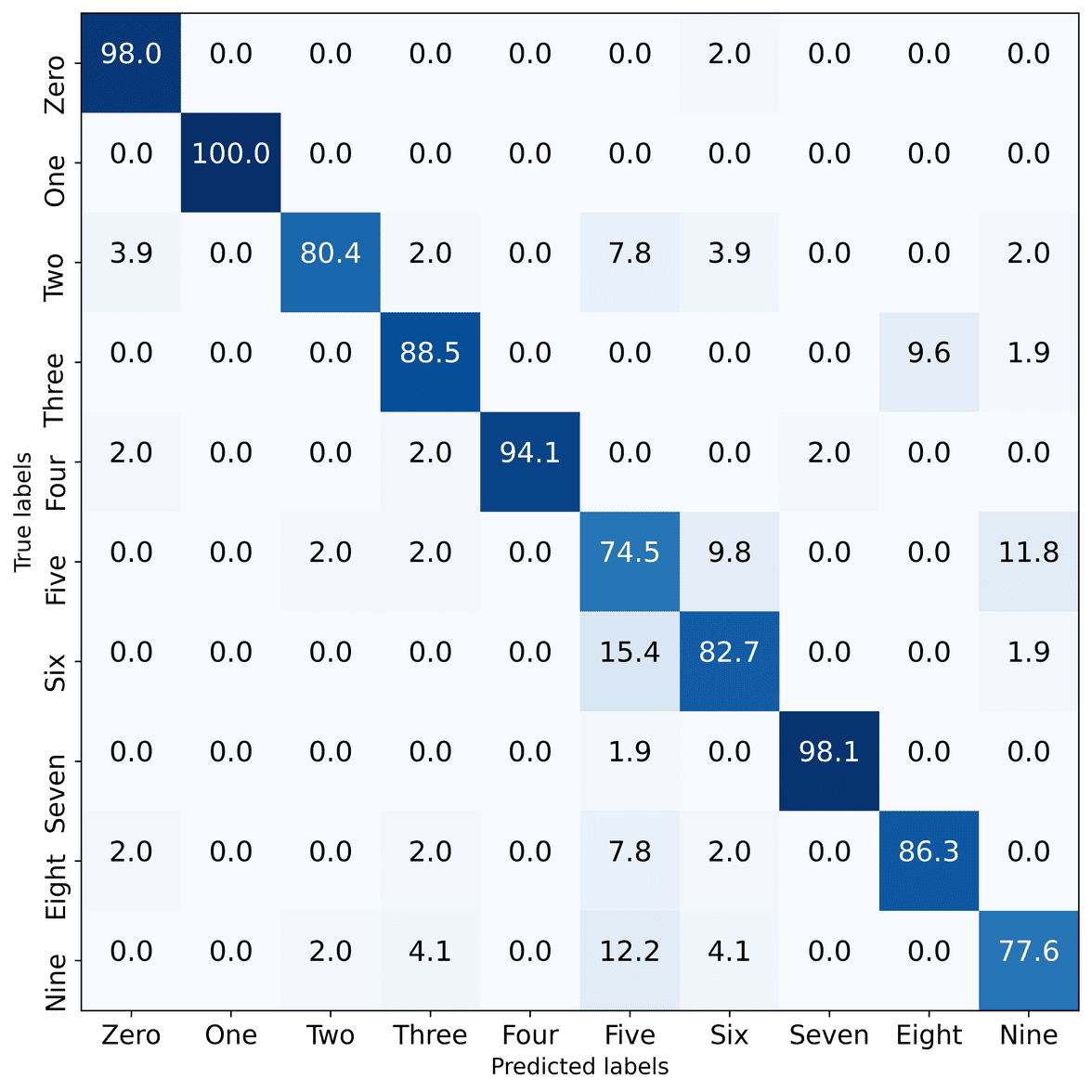
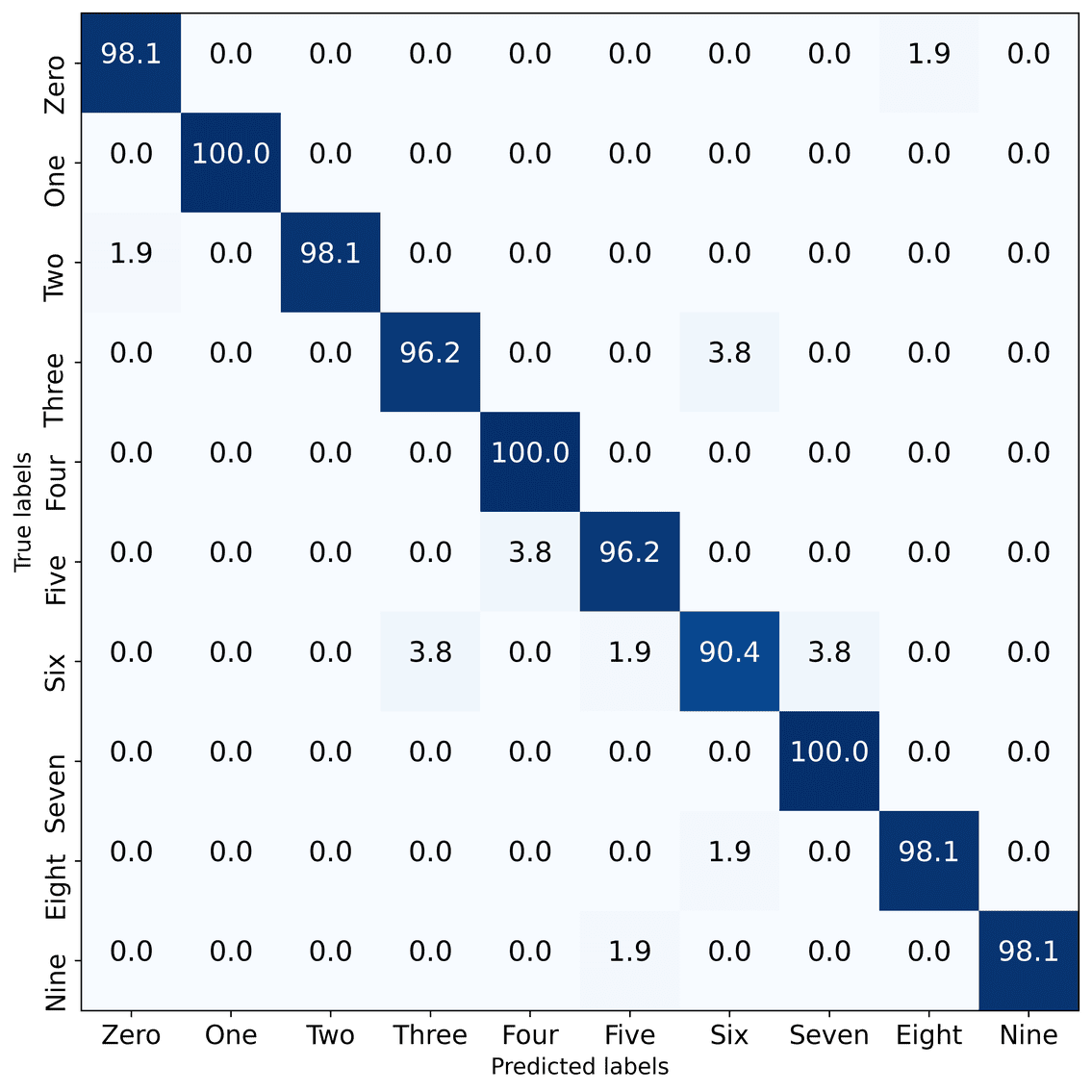
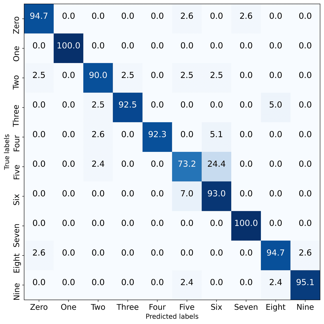
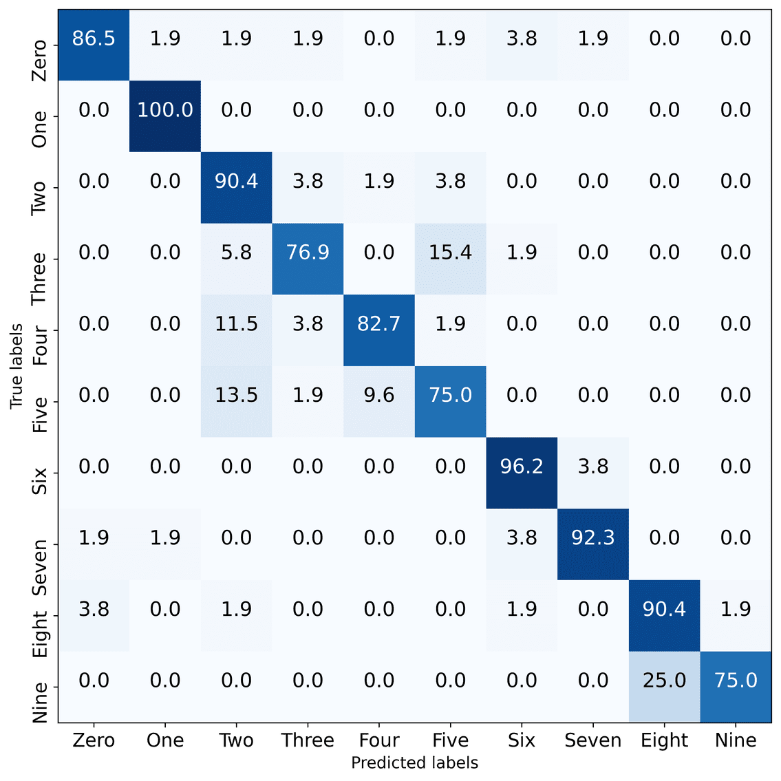
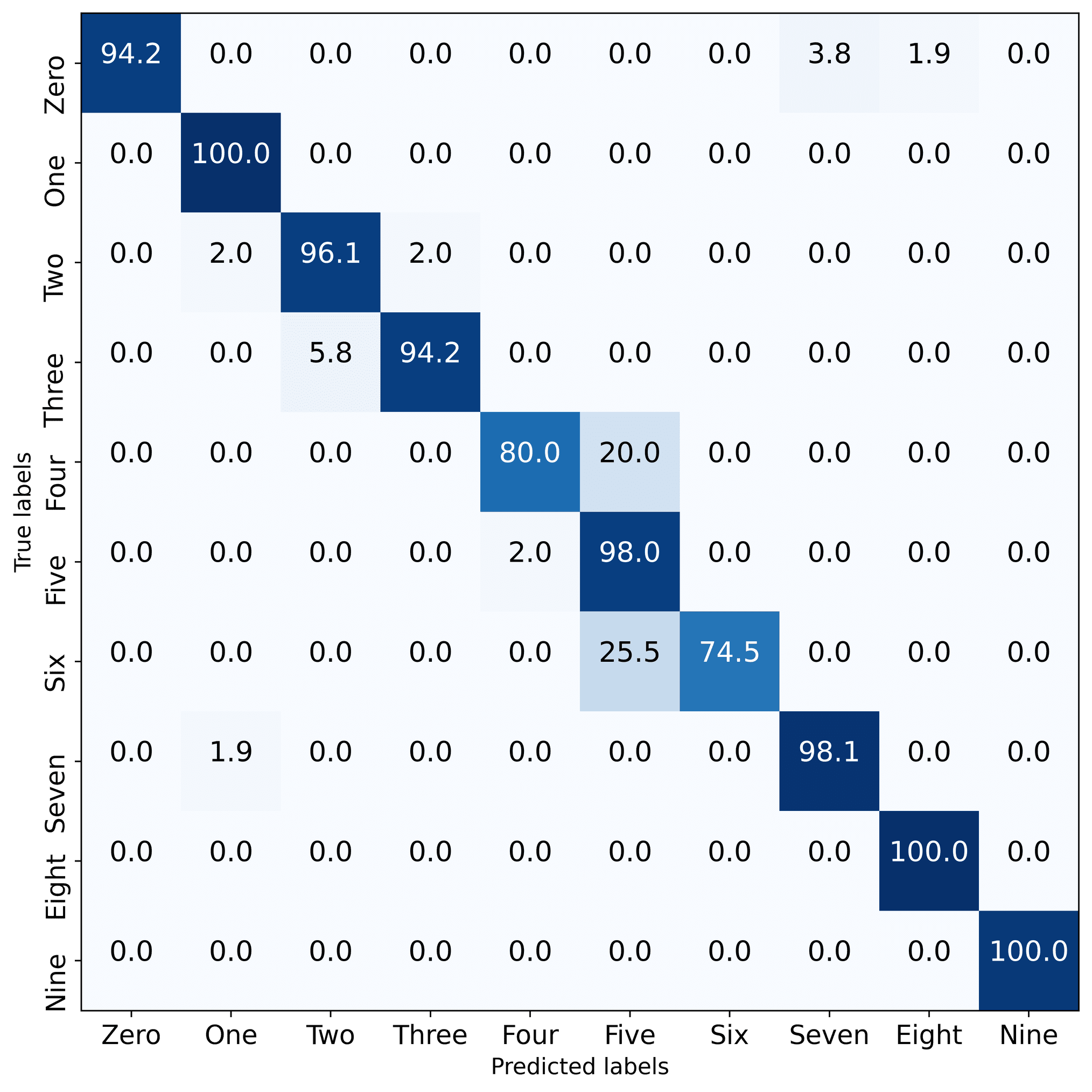
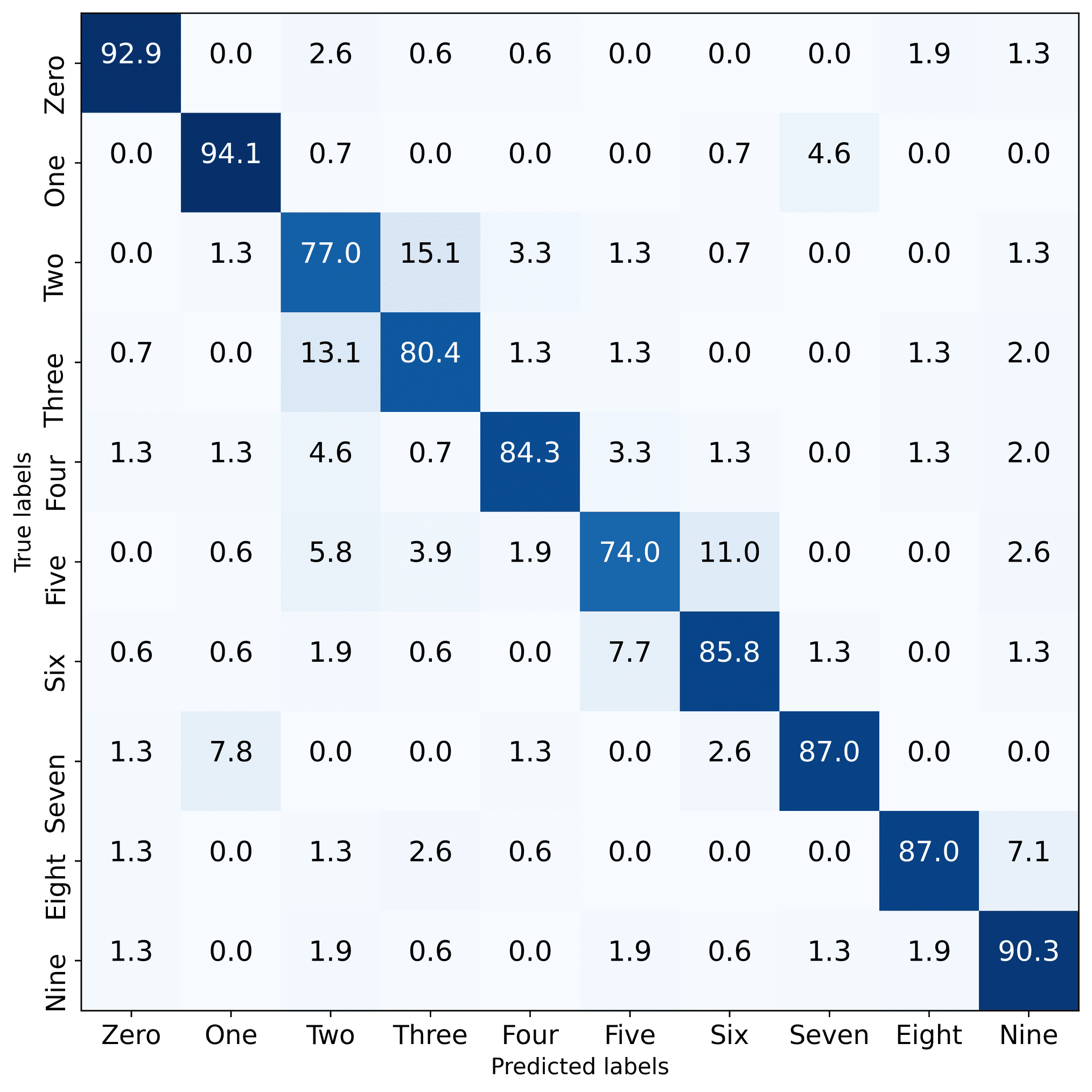
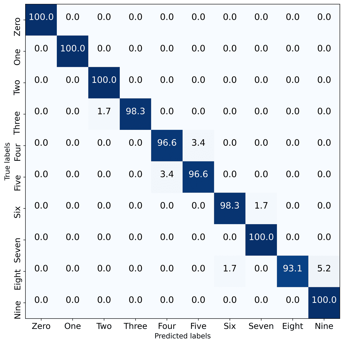
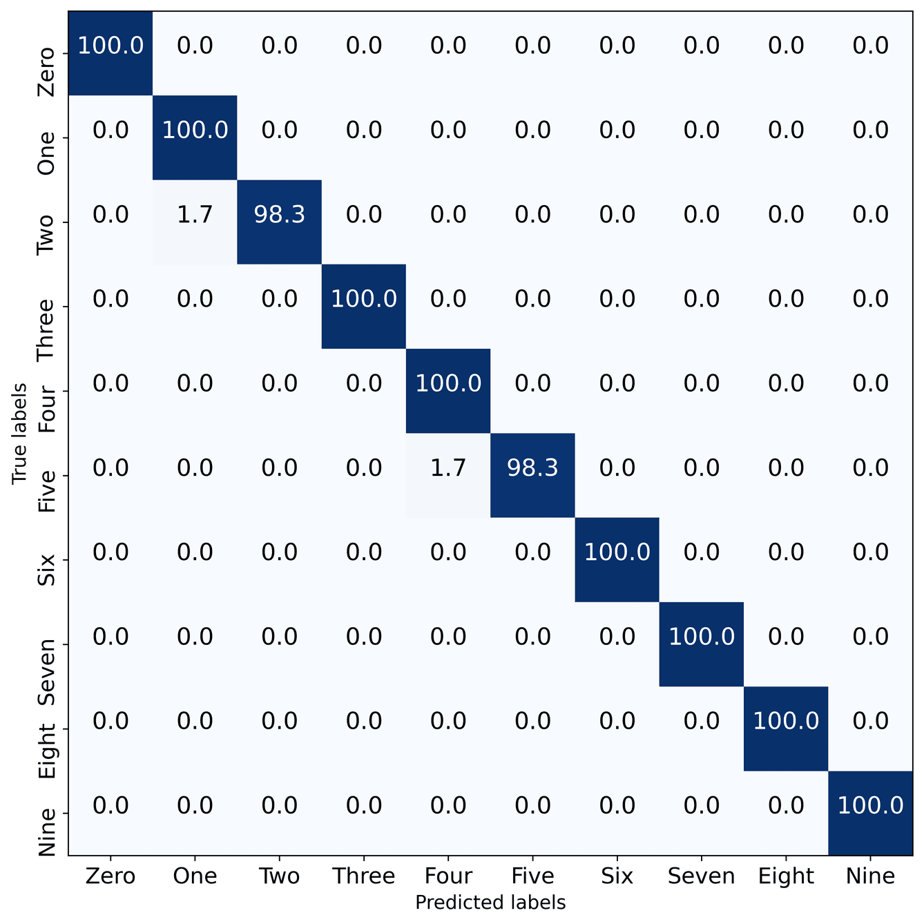
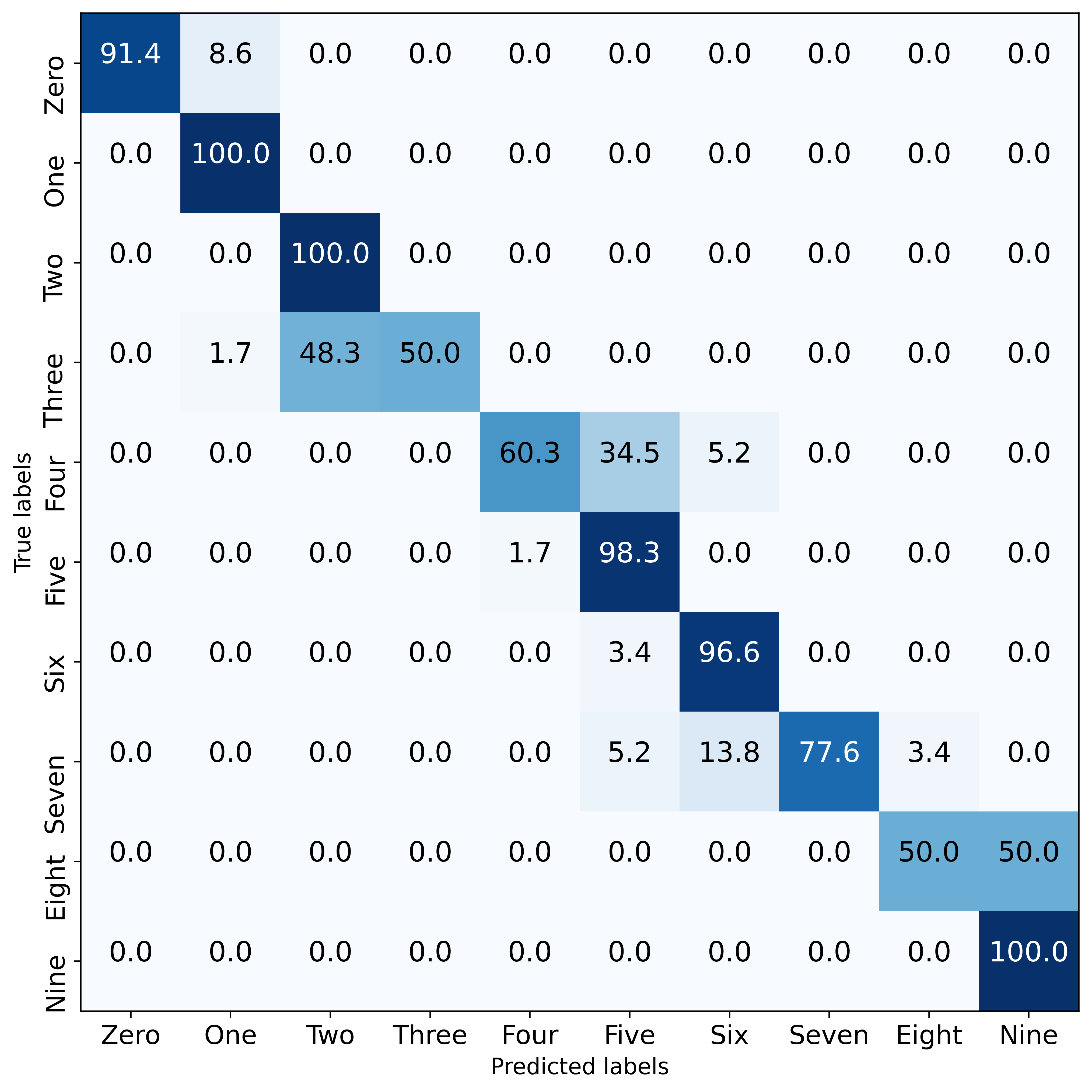
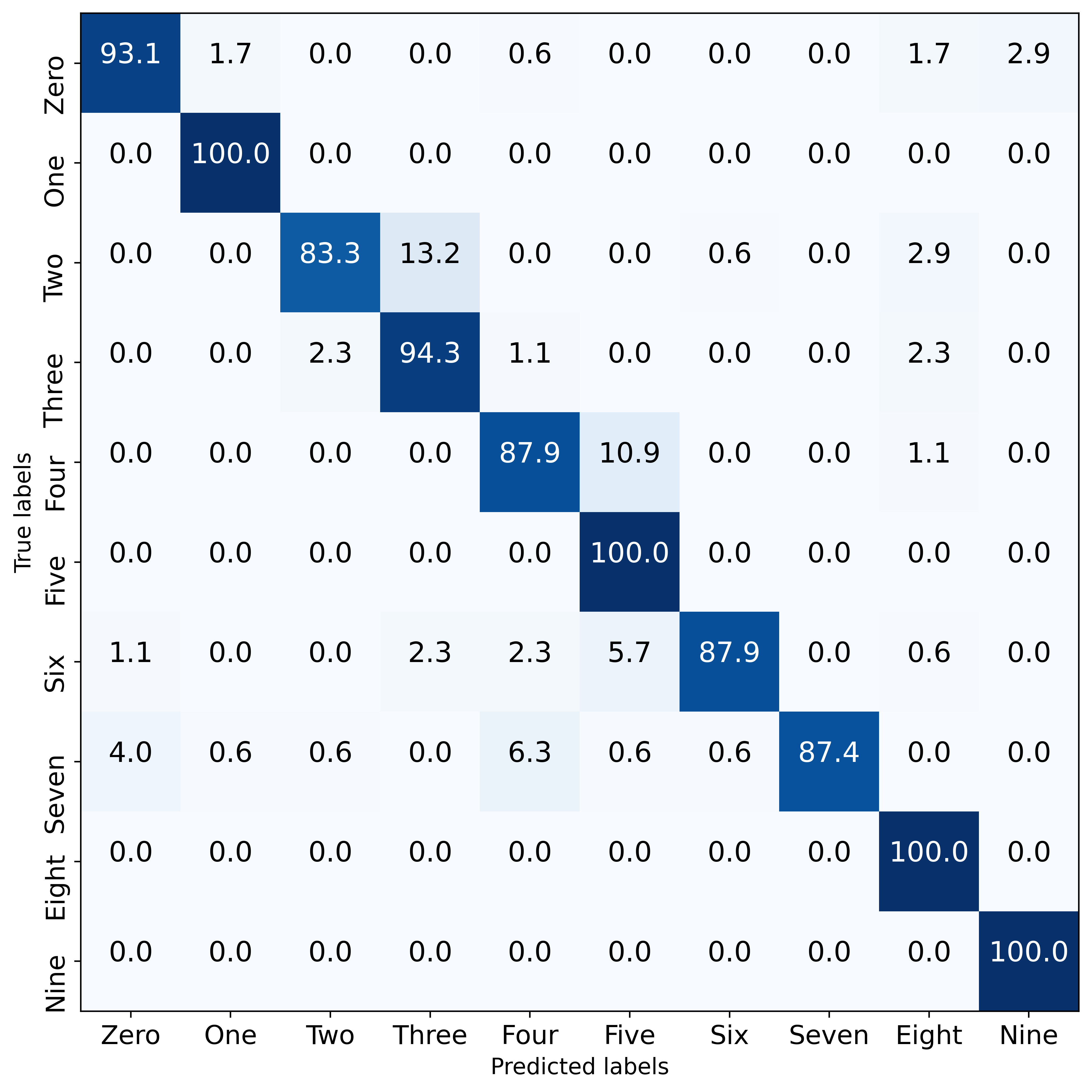
The performance of CNN and ViT models on WiFi CSI data classification for $10$ different activities is evaluated across primary combinations with varying velocities: Low, Medium, High, and all velocities. Here is a detailed review of the results presented in Tables 4 to 7, and also the confusion matrices are presented in the Appendix section.

Model WiFi modality on Low velocity Metric Zero One Two Three Four Five Six Seven Eight Nine CNN Precision 98.1$\pm$3.3 100.0$\pm$0.0 100.0$\pm$0.0 96.2$\pm$6.7 96.7$\pm$5.8 96.1$\pm$3.9 93.9$\pm$6.9 96.4$\pm$3.6 98.1$\pm$3.3 100.0$\pm$0.0 Recall 98.1$\pm$3.3 100.0$\pm$0.0 98.1$\pm$3.3 96.2$\pm$6.7 100.0$\pm$0.0 96.2$\pm$6.7 90.4$\pm$8.4 100.0$\pm$0.0 98.1$\pm$3.3 98.1$\pm$3.3 F1-Score 98.1$\pm$3.3 100.0$\pm$0.0 99.0$\pm$1.7 96.2$\pm$6.7 98.2$\pm$3.1 96.1$\pm$4.9 92.1$\pm$7.5 98.2$\pm$1.9 98.1$\pm$3.3 99.0$\pm$1.7 ViT Precision 95.0$\pm$5.3 100.0$\pm$0.0 92.6$\pm$5.1 98.1$\pm$3.3 100.0$\pm$0.0 85.4$\pm$17.1 77.6$\pm$11.0 97.5$\pm$4.3 91.4$\pm$8.8 96.4$\pm$6.2 Recall 91.9$\pm$8.6 100.0$\pm$0.0 89.9$\pm$10.7 89.7$\pm$13.7 91.7$\pm$8.3 74.9$\pm$22.6 92.5$\pm$13.0 100.0$\pm$0.0 93.1$\pm$8.2 95.3$\pm$4.8 F1-Score 93.1$\pm$5.1 100.0$\pm$0.0 90.6$\pm$4.1 93.0$\pm$7.7 95.5$\pm$4.6 76.4$\pm$16.8 83.5$\pm$9.0 98.7$\pm$2.3 92.1$\pm$7.5 95.6$\pm$2.9

Table 4: Model performance for different classes for CNN and ViT models, trained on $70\%$, validation on $10\%$ and tested on $20\%$ of the WiFi modality collected from both robotic arms at Low velocity.

For Low velocity, the CNN model generally achieves high precision, recall, and F1-scores across all classes, with precision ranging from $93.4\%$ to $100\%$, recall from $90.4\%$ to $100\%$, and F1-scores from $91.3\%$ to $100\%$. The ViT model also performs well but shows more variability, particularly in precision and recall for $A=2$ (precision: $90.6\%\pm 4.1\%$, recall: $89.9\%\pm 10.7\%$). Both models achieve perfect recall for some classes, indicating their ability to correctly identify all instances of certain activities.

Model WiFi modality on Medium velocity Metric Zero One Two Three Four Five Six Seven Eight Nine CNN Precision 93.4$\pm$7.7 96.3$\pm$3.7 91.2$\pm$9.0 85.4$\pm$9.4 100.0$\pm$0.0 92.7$\pm$5.1 100.0$\pm$0.0 91.4$\pm$5.5 98.1$\pm$3.3 98.2$\pm$3.1 Recall 90.4$\pm$6.4 92.3$\pm$5.4 90.4$\pm$6.4 94.2$\pm$3.3 100.0$\pm$0.0 94.2$\pm$3.3 98.1$\pm$3.3 96.2$\pm$3.8 96.2$\pm$3.8 88.5$\pm$12.8 F1-Score 91.3$\pm$1.0 94.1$\pm$2.1 90.5$\pm$6.1 89.3$\pm$5.3 100.0$\pm$0.0 93.4$\pm$3.0 99.0$\pm$1.7 93.5$\pm$1.5 97.1$\pm$3.2 92.4$\pm$6.8 ViT Precision $94.2\pm 5.9$ $96.7\pm 5.8$ $72.5\pm 5.6$ $87.7\pm 8.9$ $88.1\pm 8.8$ $78.5\pm 17.7$ $89.9\pm 6.9$ $94.6\pm 5.7$ $87.0\pm 22.5$ $73.2\pm 42.4$ Recall $86.5\pm 11.4$ $100.0\pm 0.0$ $90.4\pm 6.4$ $76.9\pm 12.2$ $82.7\pm 6.4$ $75.0\pm 11.4$ $96.1\pm 6.7$ $92.3\pm 7.7$ $90.4\pm 12.6$ $75.0\pm 43.3$ F1-Score $89.7\pm 6.8$ $98.2\pm 3.1$ $80.4\pm 5.4$ $81.3\pm 8.0$ $85.2\pm 6.8$ $76.3\pm 14.1$ $92.6\pm 4.6$ $93.1\pm 4.6$ $86.2\pm 15.3$ $74.1\pm 42.8$

Table 5: Model performance for different classes for CNN and ViT models, trained on $70\%$, validation on $10\%$ and tested on $20\%$ of the WiFi modality collected from both robotic arms at Medium velocity.

At Medium velocity, the performance of both models is slightly reduced compared to Low velocity. The CNN model maintains relatively high scores, with precision ranging from $85.4\%$ to $100\%$, recall from $90.4\%$ to $100\%$, and F1-scores from $85.2\%$ to $100\%$. The ViT model again shows variability, especially in $A=7$ (precision: $87.0\%\pm 22.5\%$, recall: $90.4\%\pm 12.6\%$), indicating challenges in maintaining consistent performance across all classes.

In High velocity scenarios, both models demonstrate robustness, but the ViT model generally outperforms the CNN model in precision and F1-scores for several classes. For instance, the ViT achieves $100\%$ precision and recall for $A=6$ and high precision ($100\%$) for $A=9$. The CNN model also performs well, but its precision and recall are slightly lower for certain classes compared to the ViT, such as $A=5$ (precision: $82.5\%\pm 6.5\%$, recall: $86.5\%\pm 6.4\%$).

Model WiFi modality on High velocity Metric Zero One Two Three Four Five Six Seven Eight Nine CNN Precision 92.3$\pm$9.6 96.7$\pm$5.8 93.9$\pm$3.5 100.0$\pm$0.0 96.3$\pm$3.7 82.5$\pm$6.5 91.1$\pm$5.4 98.2$\pm$3.1 100.0$\pm$0.0 94.6$\pm$5.9 Recall 100.0$\pm$0.0 100.0$\pm$0.0 88.5$\pm$3.8 100.0$\pm$0.0 94.2$\pm$6.4 86.5$\pm$6.4 92.3$\pm$9.4 100.0$\pm$0.0 86.5$\pm$11.4 92.3$\pm$9.4 F1-Score 95.7$\pm$5.5 98.2$\pm$3.1 91.1$\pm$3.3 100.0$\pm$0.0 95.1$\pm$3.4 84.1$\pm$3.8 91.3$\pm$4.8 99.1$\pm$1.6 92.4$\pm$6.8 93.0$\pm$5.3 ViT Precision 100.0$\pm$0.0 96.4$\pm$3.6 94.9$\pm$5.6 98.2$\pm$3.1 97.9$\pm$3.6 70.5$\pm$10.9 100.0$\pm$0.0 96.4$\pm$3.6 98.2$\pm$3.1 100.0$\pm$0.0 Recall 94.2$\pm$3.3 100.0$\pm$0.0 96.0$\pm$4.0 94.2$\pm$6.4 79.8$\pm$31.5 98.1$\pm$3.3 74.4$\pm$7.0 98.1$\pm$3.3 100.0$\pm$0.0 100.0$\pm$0.0 F1-Score 97.0$\pm$1.7 98.1$\pm$1.8 95.2$\pm$1.4 96.0$\pm$2.9 82.9$\pm$25.0 81.3$\pm$7.4 85.1$\pm$4.5 97.1$\pm$1.6 99.1$\pm$1.60 100.00$\pm$0.00

Table 6: Model performance for different classes for CNN and ViT models, trained on $70\%$, validation on $10\%$ and tested on $20\%$ of the WiFi modality collected from both robotic arms at High velocity.

When considering all velocities, both models show a general decline in performance, likely due to the increased variability in the data. The CNN model’s precision ranges from 78.6% to 93.5%, recall from 71.2% to 94.1%, and F1-scores from 74.5% to 92.1%. The ViT model maintains relatively high performance but with more significant standard deviations, indicating inconsistency across some classes. For example, class Two shows a significant drop in F1-score (74.2%$\pm$11.9%).

Overall, both CNN and ViT models demonstrate strong performance in classifying WiFi CSI data for various activities across different velocities. The CNN model exhibits more stable performance with smaller variations, while the ViT model occasionally achieves higher precision and recall but with greater variability. In High velocity and all-velocity scenarios, the ViT model tends to outperform the CNN model in specific metrics, suggesting its potential for handling more dynamic environments. However, the variability in the ViT’s performance indicates that further optimization may be necessary to achieve consistent results across all classes and velocities.

Model WiFi modality on All velocities Metric Zero One Two Three Four Five Six Seven Eight Nine CNN Precision 91.1$\pm$6.4 89.6$\pm$6.6 84.5$\pm$10.4 88.1$\pm$3.3 93.5$\pm$3.1 78.6$\pm$7.9 86.2$\pm$6.3 93.5$\pm$8.1 89.0$\pm$2.8 91.1$\pm$5.4 Recall 89.1$\pm$2.8 95.5$\pm$4.6 82.7$\pm$11.4 89.7$\pm$8.1 92.3$\pm$6.0 71.2$\pm$7.6 85.3$\pm$9.1 90.4$\pm$6.4 93.6$\pm$3.8 93.6$\pm$3.8 F1-Score 90.1$\pm$4.6 92.4$\pm$4.7 83.2$\pm$9.5 88.7$\pm$4.9 92.8$\pm$4.4 74.5$\pm$6.3 85.7$\pm$7.5 91.6$\pm$5.5 91.2$\pm$3.1 92.1$\pm$2.3 ViT Precision 93.6$\pm$5.1 89.4$\pm$8.1 73.4$\pm$15.3 80.1$\pm$15.3 90.2$\pm$0.6 83.3$\pm$6.0 84.5$\pm$10.1 92.4$\pm$5.8 93.1$\pm$2.0 84.6$\pm$8.3 Recall 92.9$\pm$3.3 94.1$\pm$2.9 76.9$\pm$11.4 80.3$\pm$15.9 84.4$\pm$8.6 74.1$\pm$16.6 85.9$\pm$6.6 86.9$\pm$8.4 86.9$\pm$7.2 90.3$\pm$6.3 F1-Score 93.2$\pm$3.6 91.6$\pm$5.3 74.2$\pm$11.9 78.5$\pm$10.0 86.9$\pm$4.6 77.2$\pm$9.1 84.9$\pm$7.5 89.4$\pm$6.3 89.7$\pm$3.9 87.1$\pm$5.6

Table 7: Model performance for different classes for CNN and ViT models, trained on $70\%$, validation on $10\%$ and tested on $20\%$ of the WiFi modality collected from both robotic arms at all velocities.

Video

Recognition of robot actions in videos is a challenging task that has received significant attention in the robotic research community. Unlike still image classification, the temporal component of videos provides crucial information for recognition, as many actions can be reliably identified based on motion information. In this part, we focus on robot action recognition in video data, building upon the approach recently addressed in [27], where the authors detected arm poses and utilized a deep neural network to recognize actions.
For a long time, convolution-based backbone architectures have been the cornerstone of visual modeling in computer vision[28, 29, 30]. However, a shift is occurring from CNNs to transformers [31, 25]. This change began with the introduction of the ViT [25] model, which uses a standard transformer encoder to globally model spatial relationships on non-overlapping patches. The success of ViT in image recognition has sparked interest in transformer-based architectures for video-based recognition tasks, resulting in the development of the video vision transformer (ViViT)[32]. Among all 3D CNN and transformer-based models for videos, we selected R(2+1)D [33] and ViViT, respectively, for their superior performance in action recognition tasks.
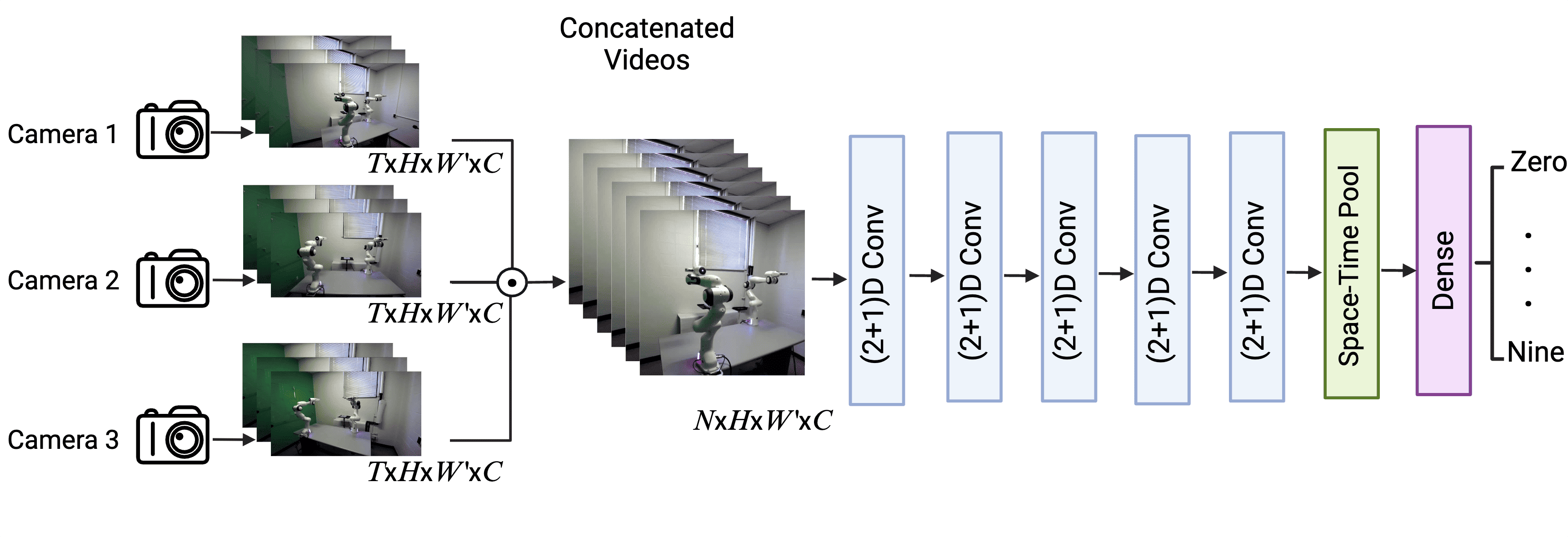
The proposed 3D CNN model for action classification is designed to effectively capture both spatial and temporal features in the input data, as illustrated in Figure 15. Each video has a duration of $15$ seconds and a frame rate of $30$ frames per second, resulting in a total of $450$ frames per video. To reduce memory usage and computational load, uniformly spaced frames are selected from each video. This uniform selection ensures consistency and simplifies batch processing. Each selected frame is concatenated along the temporal dimension to create a 4D tensor of shape $\mathbb{R}^{N\times H\times W\times C}$. In this tensor, $N$ corresponds to the number of selected frames per video, $H$ represents height, $W$ represents width, and $C$ denotes the number of channels. For training purposes, multiple video tensors are batched together, resulting in a 5D tensor with dimensions $\mathbb{R}^{B\times N\times H\times W\times C}$, where $B$ denotes the batch size. By following this structured approach, we optimize both the memory usage and computational efficiency, while ensuring that the model receives well-prepared, uniform video data for training. We outline the various stages of preprocessing as follows:

• Extracting frames: Let $\mathscr{V}$ denote a video captured from one module in this dataset, where $\mathscr{V}=\{\mathbf{F}_{1},\mathbf{F}_{2},\ldots,\mathbf{F}_{T}\}$, with $\mathbf{F}_{i}$ representing the $i$-th frame and $T$ the total number of frames in the video. Each frame $\mathbf{F}_{i}$ has dimensions $H\times W$, so $\mathbf{F}_{i}\in\mathbb{R}^{H\times W\times C}$, where $C$ is the number of channels.

• Frame sampling: For reducing temporal information and improving processing speed, we selected a subset of $N$ frames, where $N$ represents the number of frames sampled from each video. The selected subset is

  $$\mathscr{F}_{j}=\{\mathbf{F}_{j1},\mathbf{F}_{j2},\ldots,\mathbf{F}_{jN}\},\quad\text{where}\quad N\leq T\quad\text{and}\quad N\in\mathbb{N}.$$ (4)

• Splitting and resizing video frames: To augment the dataset, each frame from a stereo-type video, which features two lenses, is split into two parts: one corresponding to the left lens and one to the right lens. This approach is feasible because 3D reconstruction or depth information is not utilized in this process, it remains accessible for further research. This separation allows each part to be processed independently, effectively doubling the dataset size and enhancing its diversity. Consequently, each frame $\mathscr{F}_{j}$ is split and then resized into dimensions $H\times W^{\prime}$ resulting in $\mathscr{F}_{j}^{\prime}\in\mathbb{R}^{H\times W^{\prime}\times C}$ frames, where $W^{\prime}=\frac{W}{2}$.

Thus, each sample in the dataset is defined with the shape $\mathbf{X}\in\mathbb{R}^{N\times H\times W^{\prime}\times C}$. Correspondingly, the training set, denoted as $\mathscr{X}_{\text{train}}$, is structured with the shape $\mathscr{X}_{\text{train}}\in\mathbb{R}^{B\times N\times H\times W^{\prime}\times C}$.
We then utilized an R(2+1)D model, employing a 2D convolution followed by a 1D convolution. This approach effectively decomposes spatial and temporal modeling into two distinct stages. The network architecture, known as R(2+1)D, consists of (2+1)D blocks.
The proposed action classification model starts with an input layer handling video data of shape $\mathbb{R}^{B\times N\times H\times W^{\prime}\times C}$. The initial layer is a 2D convolution followed by a 1D convolution with 16 filters, a kernel size of $(3,7,7)$, ’same’ padding, followed by batch normalization and ReLU activation, designed to process both spatial and temporal features. The output is then resized to half the original height and width.
Following this, the model includes four residual blocks. The first residual block comprises two (2+1)D convolutions layers, each with 16 filters and a kernel size of $(3,3,3)$, ’same’ padding, followed by layer normalization and ReLU activation, and concludes with a resizing layer that reduces the spatial dimensions to a quarter of the original size. The subsequent residual blocks have similar structures but with increasing filters: 32 filters for the second block, 64 filters for the third block, and 128 filters for the fourth block, with each block further reducing the spatial dimensions. After the residual blocks, a global average pooling layer aggregates the features across the entire spatial-temporal volume, followed by a flattening layer. The model concludes with a dense layer comprising $10$ units, corresponding to the classification output for the $10$ activity classes performed by both robots. The model was trained over $50$ epochs with early stopping patience set to $10$ based on validation accuracy, a batch size of $8$, and an Adam optimizer with a learning rate of $1\times 10^{-4}$. This configuration aims to optimize performance while ensuring robust generalization to unseen video data.
This architecture offers notable advantages over full 3D convolution. Firstly, it effectively doubles the network’s nonlinearities by introducing an additional ReLU activation between the 2D and 1D convolutions within each block, without increasing the parameter count. Secondly, decomposing the 3D convolution into separate spatial and temporal components simplifies the optimization process. A major benefit of this method is the reduction in the number of parameters, which enhances both computational efficiency and overall performance[33].

Figure 15: Different steps of training 3D CNN model from extracting $N=10$ frames from each video to classification.

Figure 16: Different steps of training ViViT model from extracting $N=10$ frames from each video to classification.

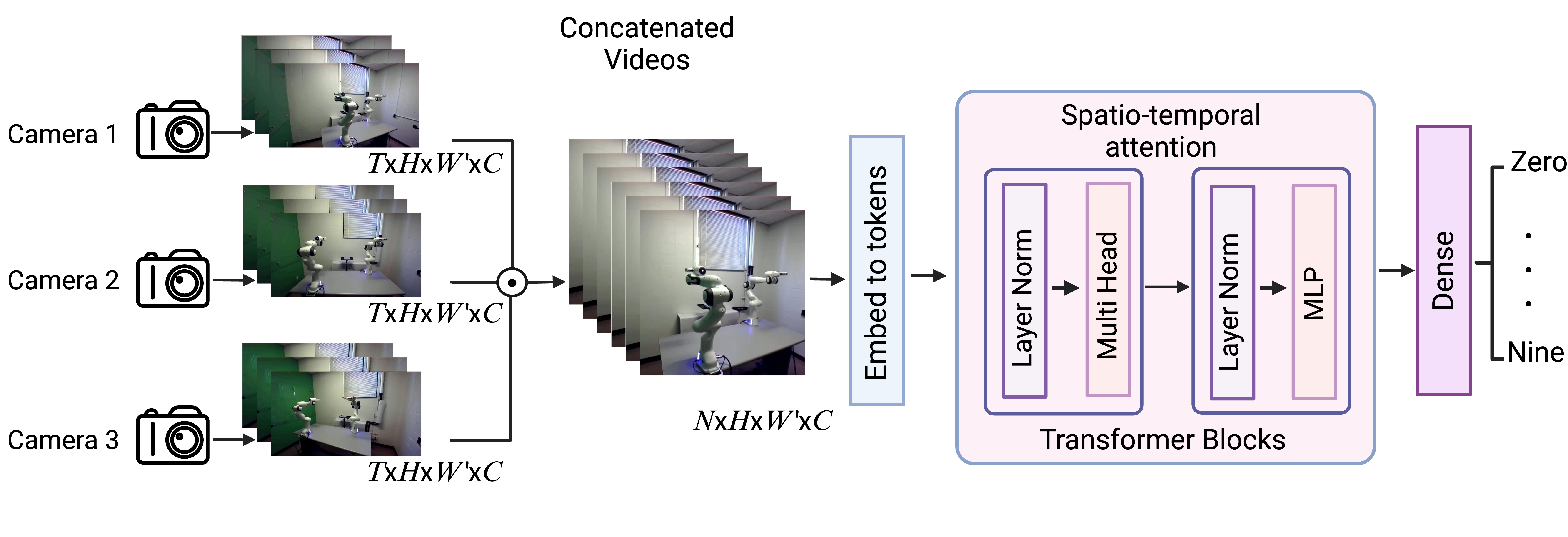
In addition, we utilized a ViViT model to introduce diversity and explore new experimental avenues. In ViTs, an image is divided into patches, which are then spatially flattened in a process known as tokenization. Since the transformer [34], which forms the foundation of ViT, is a flexible architecture capable of processing any sequence of input tokens, we utilized one of four variants of the vision transformer to tokenize the video.
We considered tubelet embedding method We employed the tubelet embedding method to convert the video into a sequence of tokens. Afterward, we added positional embeddings to the tokens, reshaped the sequence, and then fed it into the transformer block [32].
Tubelet Embedding captures temporal information from the video. Initially, volumes are extracted from the video, each containing patches of frames along with temporal data. These volumes are then flattened to construct video tokens, to which positional information is added. Among the four variants of the vision transformer, we implemented the Spatio-temporal attention model for its simplicity. This model employs a custom tubelet embedding layer, which uses 3D convolution with a patch size of $(18,18,18)$ to project video patches into a $256$-dimensional embedding space, and a positional encoder layer that adds positional information to these tokens. The core of the model consists of eight transformer layers, each featuring layer normalization with an epsilon of $1\times 10^{-6}$, multi-head self-attention with eight heads, and feed-forward networks with Gaussian Error Linear Unit (GELU) activations and skip connections. The model processes input data shaped $\mathbb{R}^{N\times H\times w^{\prime}\times C}$ and classifies into 10 classes of activities. It is compiled with the Adam optimizer, using a learning rate of $1\times 10^{-4}$ and a weight decay of $1\times 10^{-5}$, and trained over $20$ epochs with a batch size of $32$. This architecture ensures robust performance and high accuracy, optimized through sparse categorical cross-entropy loss and leveraging TensorFlow’s AUTOTUNE for efficient data handling. The architecture of the model is illustrated in Figure 16. For this purpose, we divide the dataset into training, validation, and test sets with a $70$%, $15$%, and $15$% split, respectively. 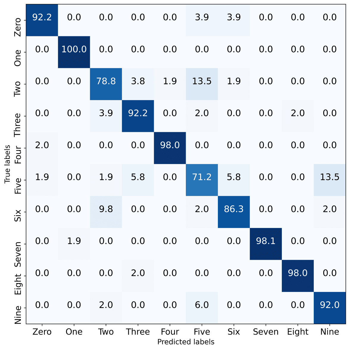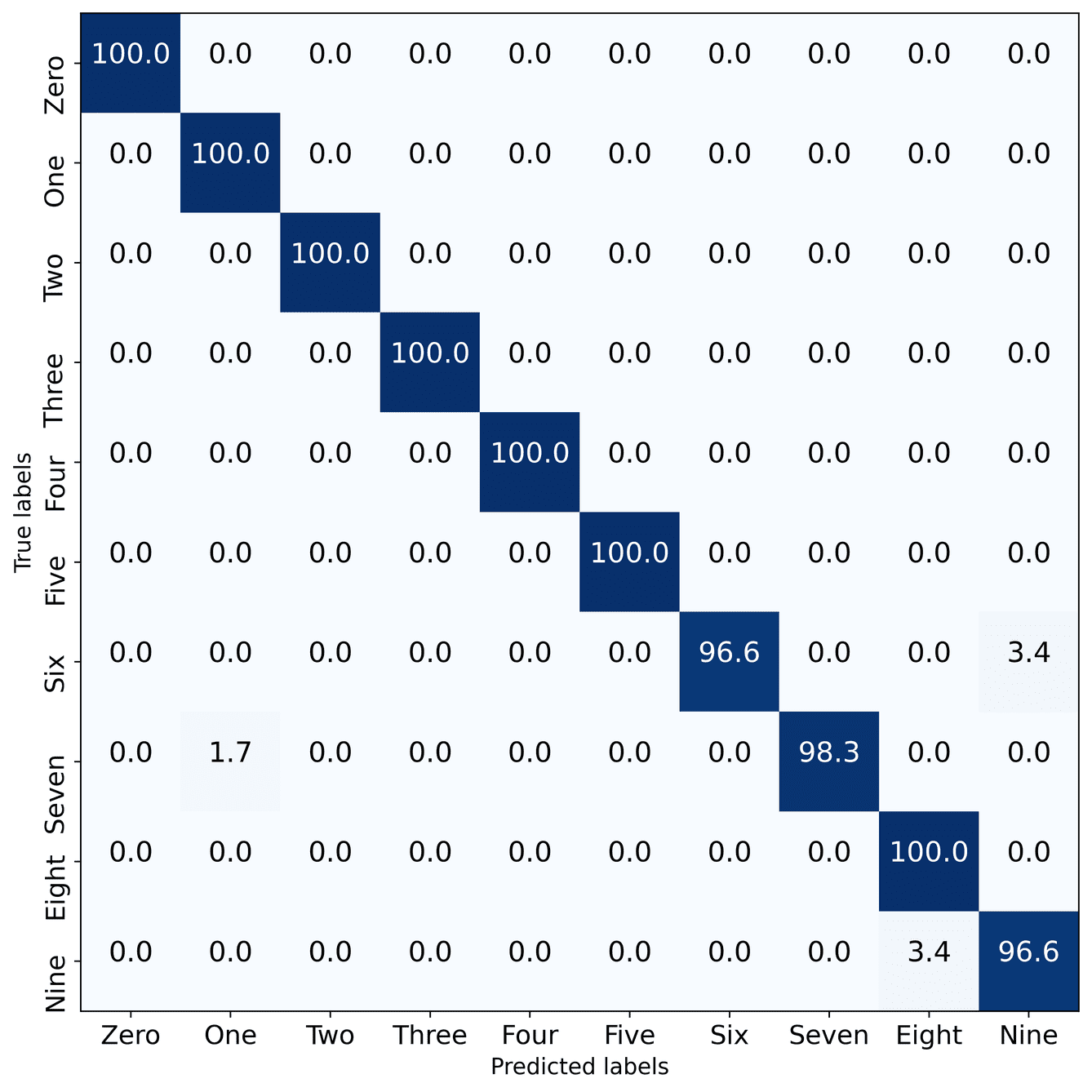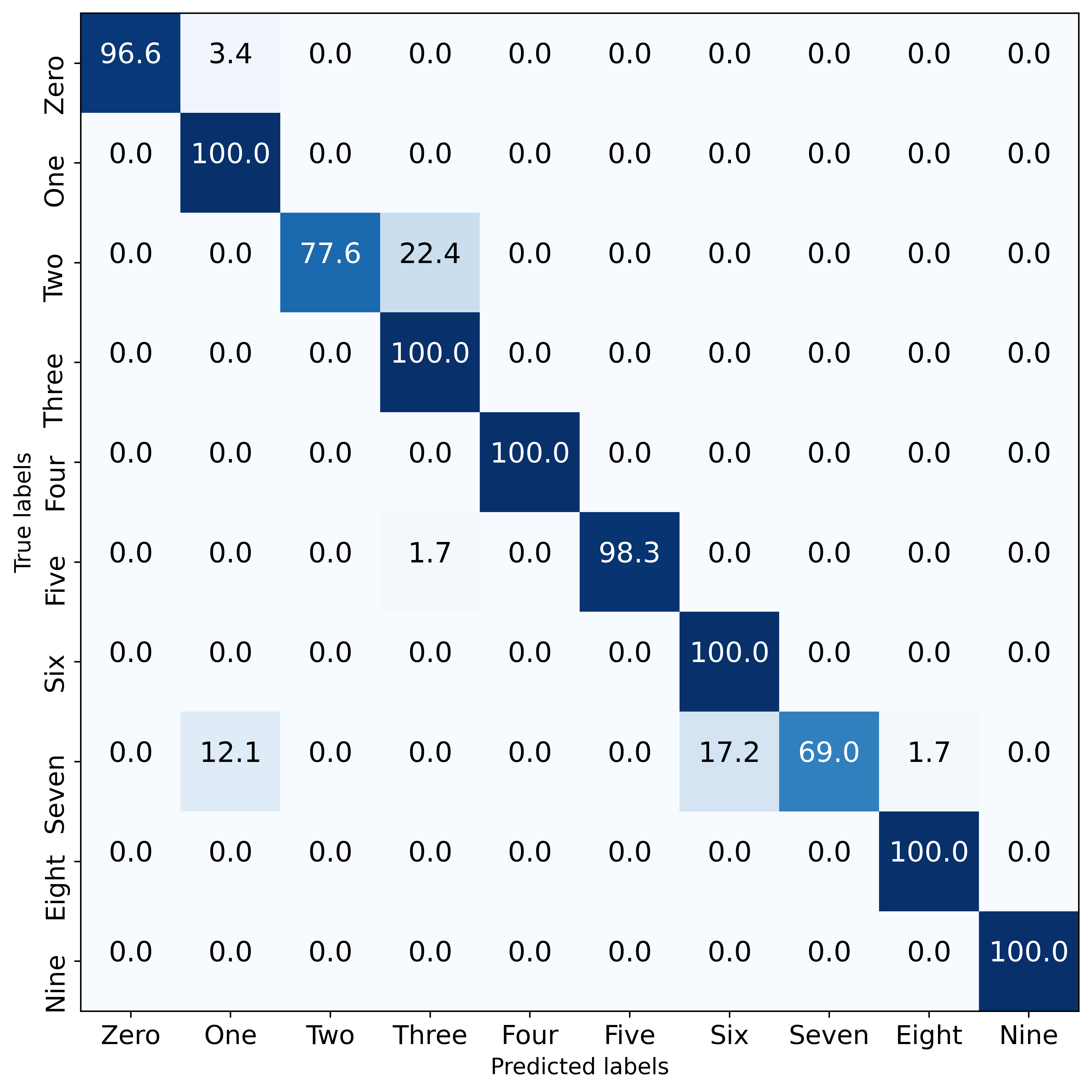Below is a comprehensive analysis of the results shown in Tables 8 to 11. The confusion matrices can be found in the Appendix.

Model Video modality on Low velocity Metric Zero One Two Three Four Five Six Seven Eight Nine 3D CNN Precision 98.2$\pm$1.6 100.0$\pm$0.3 100.0$\pm$1.9 98.3$\pm$1.1 100.0$\pm$0.6 100.0$\pm$1.8 100.0$\pm$0.8 100.0$\pm$1.2 98.3$\pm$1.4 96.7$\pm$0.8 Recall 96.6$\pm$0.5 100.0$\pm$1.3 96.6$\pm$1.3 100.0$\pm$0.6 100.0$\pm$1.2 100.0$\pm$1.0 100.0$\pm$1.5 100.0$\pm$1.1 100.0$\pm$0.6 98.3$\pm$1.4 F1-Score 97.4$\pm$1.4 100.0$\pm$0.9 98.2$\pm$1.3 99.1$\pm$0.7 100.0$\pm$1.5 100.0$\pm$0.9 100.0$\pm$1.2 100.0$\pm$1.8 99.1$\pm$1.5 97.4$\pm$0.9 ViViT Precision 100.0$\pm$1.8 87.2$\pm$2.1 100.0$\pm$1.3 81.4$\pm$2.2 100.0$\pm$0.3 100.0$\pm$2.8 85.0$\pm$2.9 100.0$\pm$2.9 98.8$\pm$3.8 100.0$\pm$1.6 Recall 97.8$\pm$3.1 100.0$\pm$1.7 78.9$\pm$3.3 100.0$\pm$4.9 100.0$\pm$1.6 98.0$\pm$2.7 100.0$\pm$1.5 69.5$\pm$3.6 100.0$\pm$2.4 100.0$\pm$1.8 F1-Score 98.9$\pm$2.4 93.1$\pm$1.8 88.2$\pm$1.5 89.7$\pm$2.8 100.0$\pm$1.0 99.0$\pm$1.3 91.9$\pm$2.1 82.0$\pm$3.1 99.4$\pm$2.2 100.0$\pm$1.2

Table 8: Model performance for different classes for 3D CNN and ViViT models, trained on $70\%$, validation on $15\%$ and tested on $15\%$ of the video modality collected from both robotic arms at Low velocity.

Model Video modality on Medium velocity Metric Zero One Two Three Four Five Six Seven Eight Nine 3D CNN Precision 100.0$\pm$1.6 98.3$\pm$1.4 100.0$\pm$0.9 98.3$\pm$0.7 100.0$\pm$1.5 100.0$\pm$1.2 100.0$\pm$1.0 100.0$\pm$1.9 96.7$\pm$1.2 96.6$\pm$0.9 Recall 100.0$\pm$1.2 100.0$\pm$1.1 100.0$\pm$0.0 100.0$\pm$1.3 100.0$\pm$0.8 100.0$\pm$1.0 96.6$\pm$0.7 98.3$\pm$1.5 100.0$\pm$1.4 96.6$\pm$1.0 F1-Score 100.0$\pm$1.7 99.1$\pm$0.8 100.0$\pm$0.1 99.1$\pm$1.6 100.0$\pm$1.1 100.0$\pm$1.9 98.2$\pm$1.2 99.1$\pm$1.8 98.3$\pm$0.9 96.6$\pm$1.5 ViViT Precision 60.4$\pm$3.2 94.1$\pm$0.9 100.0$\pm$1.8 100.0$\pm$2.2 100.0$\pm$3.1 100.0$\pm$3.6 78.7$\pm$4.1 100.0$\pm$2.5 74.6$\pm$1.4 100.0$\pm$3.9 Recall 100.0$\pm$1.0 100.0$\pm$2.9 100.0$\pm$2.6 100.0$\pm$4.1 100.0$\pm$0.4 95.0$\pm$4.2 60.8$\pm$2.9 81.7$\pm$3.1 93.8$\pm$2.1 47.8$\pm$5.5 F1-Score 75.3$\pm$2.1 96.9$\pm$1.4 100.0$\pm$2.2 100.0$\pm$2.4 100.0$\pm$1.6 97.4$\pm$3.2 68.7$\pm$3.0 89.9$\pm$2.8 83.1$\pm$1.9 64.7$\pm$3.7

Table 9: Model performance for different classes for 3D CNN and ViViT models, trained on $70\%$, validation on $15\%$ and tested on $15\%$ of the video modality collected from both robotic arms at Medium velocity.

Model Video modality on High velocity Metric Zero One Two Three Four Five Six Seven Eight Nine 3D CNN Precision 100.0$\pm$0.5 100.0$\pm$0.4 98.3$\pm$1.2 100.0$\pm$1.3 96.6$\pm$1.4 96.6$\pm$2.0 98.3$\pm$1.5 98.3$\pm$1.1 100.0$\pm$0.7 95.1$\pm$1.8 Recall 100.0$\pm$1.3 100.0$\pm$1.1 100.0$\pm$1.4 98.3$\pm$1.2 96.6$\pm$1.9 96.6$\pm$1.2 98.3$\pm$0.7 100.0$\pm$1.0 93.1$\pm$1.6 100.0$\pm$1.4 F1-Score 100.0$\pm$1.1 100.0$\pm$1.0 99.2$\pm$1.5 99.1$\pm$1.2 96.6$\pm$0.8 96.6$\pm$1.6 98.3$\pm$1.4 99.2$\pm$1.3 96.4$\pm$1.8 97.5$\pm$1.1 ViViT Precision 100.0$\pm$3.7 91.4$\pm$4.9 67.5$\pm$2.3 100.0$\pm$2.9 97.5$\pm$3.1 70.6$\pm$2.8 84.0$\pm$4.1 100.0$\pm$0.9 94.3$\pm$2.7 67.2$\pm$3.0 Recall 91.9$\pm$3.2 100.0$\pm$4.7 100.0$\pm$3.2 50.4$\pm$4.3 60.8$\pm$3.9 98.4$\pm$1.7 97.3$\pm$1.9 78.5$\pm$4.6 50.3$\pm$4.1 100.0$\pm$4.7 F1-Score 95.8$\pm$2.1 95.5$\pm$2.8 80.6$\pm$3.1 67.0$\pm$3.7 74.9$\pm$3.5 82.5$\pm$3.0 90.1$\pm$4.2 87.9$\pm$2.5 66.1$\pm$2.9 80.4$\pm$3.6

Table 10: Model performance for different classes for 3D CNN and ViViT models, trained on $70\%$, validation on $15\%$ and tested on $15\%$ of the video modality collected from both robotic arms at High velocity.

Model Video modality on All velocities Metric Zero One Two Three Four Five Six Seven Eight Nine 3D CNN Precision 100.0$\pm$1.5 98.3$\pm$1.4 100.0$\pm$1.1 100.0$\pm$1.3 98.3$\pm$1.8 100.0$\pm$0.9 100.0$\pm$1.4 100.0$\pm$1.6 100.0$\pm$1.1 100.0$\pm$1.5 Recall 100.0$\pm$0.8 100.0$\pm$1.1 98.3$\pm$1.2 100.0$\pm$1.7 100.0$\pm$0.9 98.3$\pm$1.3 100.0$\pm$1.2 100.0$\pm$1.4 100.0$\pm$1.0 100.0$\pm$1.2 F1-Score 100.0$\pm$0.9 99.2$\pm$1.2 99.1$\pm$1.4 100.0$\pm$1.1 99.2$\pm$1.5 99.1$\pm$1.8 100.0$\pm$1.3 100.0$\pm$1.7 100.0$\pm$1.1 100.0$\pm$0.8 ViViT Precision 95.2$\pm$2.3 98.4$\pm$2.1 97.9$\pm$2.6 86.3$\pm$1.7 89.1$\pm$3.8 85.6$\pm$2.7 99.4$\pm$1.2 100.0$\pm$2.9 92.7$\pm$1.8 97.3$\pm$1.9 Recall 93.6$\pm$3.8 100.0$\pm$1.7 83.5$\pm$3.2 94.4$\pm$2.7 88.7$\pm$2.6 100.0$\pm$0.8 88.3$\pm$2.1 87.6$\pm$3.1 100.0$\pm$1.1 100.0$\pm$1.0 F1-Score 94.4$\pm$3.1 99.2$\pm$2.9 90.1$\pm$3.4 90.2$\pm$2.7 88.9$\pm$3.5 92.3$\pm$2.8 93.5$\pm$3.1 93.4$\pm$2.5 96.2$\pm$2.0 98.6$\pm$2.1

Table 11: Model performance for different classes for 3D CNN and ViViT models, trained on $70\%$, validation on $15\%$ and tested on $15\%$ of the video modality collected from both robotic arms at all velocities.

Audio

To analyze the audio data, we preprocess each audio sample by computing their spectrograms. The short-time Fourier transform (STFT) is employed to convert the audio signal from the time domain to the frequency domain. For this transformation, we use a fast Fourier transform (FFT) size $n_{fft}$ of $512$ and a hop length of 256. The resulting spectrogram has dimensions that depend on the FFT size and the hop length. The number of frequency bins $F$ in the spectrogram is calculated as $\frac{n_{fft}}{2}+1$, which equals 257 for an FFT size of $512$. The number of time frames is determined by dividing the total number of samples by the hop length. For our audio files, this yields approximately 2,583 time frames ($\frac{661,500}{256}\approx 2{,}583$). To ensure consistency in the dimensions of the spectrograms, we limit the number of time frames to a maximum of $T^{\prime}$, which in this paper is set to $2{,}555$. If the number of frames exceeds this limit, the spectrogram is trimmed from both sides equally by removing an equal number of frames from the beginning and the end of the spectrogram. After this adjustment, the final dimensions of the spectrogram are $257$ frequency bins and up to $2{,}555$ time frames. This preprocessing ensures that all spectrograms have consistent dimensions, facilitating subsequent analysis.

Figure 17: Different steps of training CNN model, from audio collection to classification.

These spectrograms are then concatenated, resulting in $1920$ combined samples, from both robotic arms. We divide the dataset into training, validation, and test sets in a $70$%, $10$%, and $20$% ratio, respectively. We implement a CNN model to classify the data into $10$ classes corresponding to the activities performed by both robots, where the architecture of the model is shown in Figure 17. The CNN model comprises two convolutional layers, the first layer is followed by a max-pooling layer, and includes a dropout layer to mitigate overfitting, with a rate of $0.5$. The final layer is a fully connected layer that outputs the class probabilities. The model is trained over $60$ epochs with a batch size of $16$, using a learning rate of $1\times 10^{-3}$ and a weight decay of $1\times 10^{-4}$ to optimize performance.

Figure 18: Different steps of training ViT model, from audio collection to classification.

We also use a ViT model as the model diversity experiment. The preprocessing handles spectrograms and labels and includes functionality to divide each image into smaller patches of a specified size. This task is essential for preparing the data in a format suitable for the ViT model. The ViT model is designed to handle data patches, embedding them into a higher-dimensional space using a linear layer. The embedded patches are then processed through a series of transformer encoder layers, which consist of multi-head self-attention mechanisms and feed-forward neural networks. The model includes a final fully connected layer to produce the class predictions, and the hyperparameters are chosen using grid search. The model is trained over $90$ epochs with a batch size of $16$, an embedding dimension of $128$, $4$ attention heads, and $6$ transformer layers, as shown in Figure 18. A dropout rate of $0.45$ is applied to prevent overfitting, and the model uses a learning rate of $1\times 10^{-4}$ with a weight decay of $1\times 10^{-5}$.

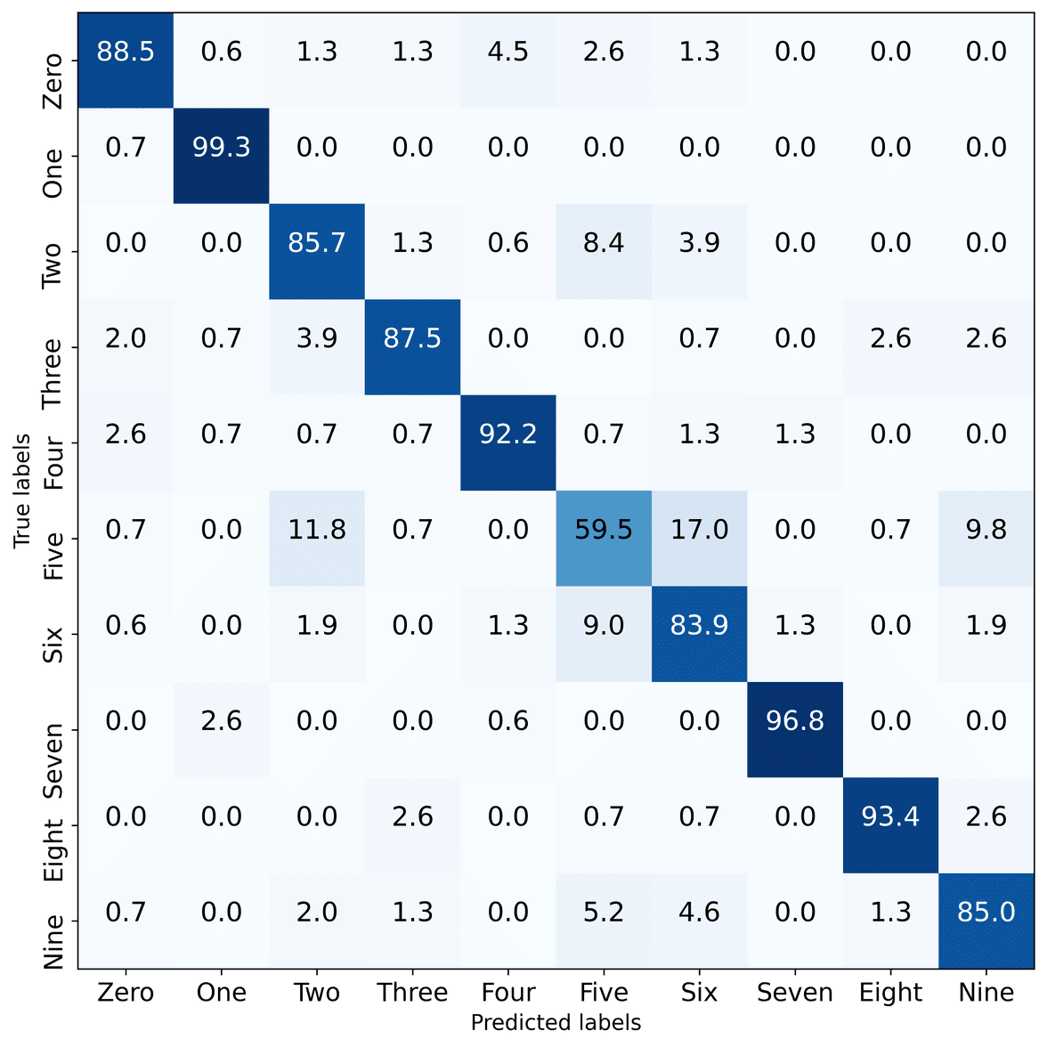
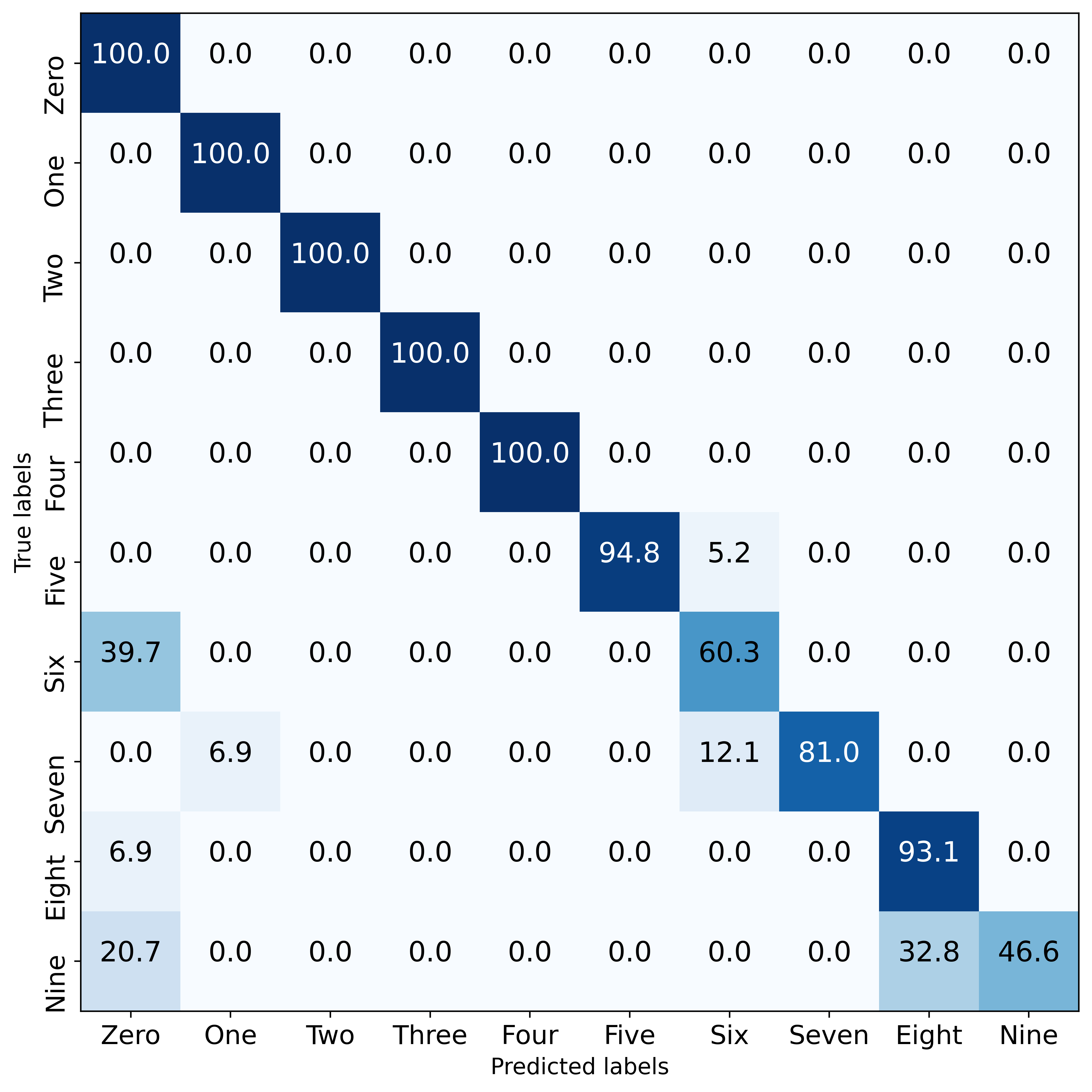
The performance of CNN and ViT models on audio data classification is evaluated across datasets with varying velocities: Low, Medium, High, and all velocities. Here is a detailed review of the results presented in Tables 12 to 15.

Model Audio modality on Low velocity Metric Zero One Two Three Four Five Six Seven Eight Nine CNN Precision 98.2$\pm$3.1 100.0$\pm$0.0 77.5$\pm$16.9 100.0$\pm$0.0 94.2$\pm$3.3 61.3$\pm$5.3 85.6$\pm$7.1 96.4$\pm$3.6 93.0$\pm$4.7 80.2$\pm$11.5 Recall 96.0$\pm$4.0 96.0$\pm$4.0 50.0$\pm$8.6 90.4$\pm$6.4 94.2$\pm$3.3 72.9$\pm$15.7 82.2$\pm$6.8 100.0$\pm$0.0 98.1$\pm$3.3 100.0$\pm$0.0 F1-Score 97.0$\pm$1.8 97.9$\pm$2.1 60.7$\pm$11.4 94.8$\pm$3.5 94.2$\pm$1.8 66.1$\pm$8.9 83.8$\pm$6.7 98.1$\pm$1.9 95.4$\pm$3.1 88.6$\pm$6.7 ViT Precision 92.9$\pm$8.2 96.2$\pm$3.8 92.0$\pm$8.0 86.3$\pm$4.6 94.4$\pm$3.3 61.3$\pm$13.4 90.1$\pm$10.2 100.0$\pm$0.0 89.3$\pm$6.2 94.7$\pm$5.3 Recall 86.4$\pm$6.2 100.0$\pm$0.0 65.4$\pm$15.9 98.1$\pm$3.3 96.2$\pm$6.7 86.2$\pm$8.5 78.8$\pm$3.3 96.2$\pm$3.8 94.2$\pm$3.3 73.1$\pm$8.6 F1-Score 89.0$\pm$2.7 98.0$\pm$2.0 74.4$\pm$8.4 91.8$\pm$3.8 95.0$\pm$1.9 70.4$\pm$7.4 83.9$\pm$5.8 98.0$\pm$2.0 91.5$\pm$2.9 82.4$\pm$7.4

Table 12: Model performance for different classes for CNN and ViT models, trained on $70\%$, validation on $10\%$ and tested on $20\%$ of the audio modality collected from both robotic arms at Low velocity.

For the Low velocity audio data, the CNN model generally achieves high precision, recall, and F1-scores across most classes, with precision ranging from $61.3\%$ to $100\%$, recall from $72.9\%$ to $100\%$, and F1-scores from $66.1\%$ to $100\%$. The ViT model also performs well, showing some variability, especially in precision and recall for $A=2$ (precision: $92.9\%\pm 8.2\%$, recall: $65.4\%\pm 15.9\%$). Both models achieve perfect recall for some classes, demonstrating their capability to accurately identify specific activities.

Model Audio modality on Medium velocity Metric Zero One Two Three Four Five Six Seven Eight Nine CNN Precision 92.4$\pm$0.5 96.0$\pm$4.0 83.8$\pm$6.5 84.6$\pm$11.9 98.1$\pm$3.3 73.5$\pm$10.5 69.5$\pm$13.8 100.0$\pm$0.0 93.9$\pm$6.9 80.5$\pm$4.8 Recall 96.0$\pm$4.0 92.3$\pm$5.4 71.0$\pm$14.5 88.3$\pm$8.5 96.0$\pm$4.0 64.9$\pm$15.5 84.3$\pm$5.5 100.0$\pm$0.0 84.6$\pm$7.7 86.5$\pm$11.4 F1-Score 94.1$\pm$2.2 94.0$\pm$3.5 76.2$\pm$10.1 86.0$\pm$8.8 97.0$\pm$3.2 68.2$\pm$12.6 75.5$\pm$10.2 100.0$\pm$0.0 88.8$\pm$6.0 83.0$\pm$6.9 ViT Precision 92.9$\pm$5.1 100.0$\pm$0.0 96.0$\pm$4.0 88.6$\pm$3.4 100.0$\pm$0.0 63.1$\pm$5.9 82.9$\pm$12.4 98.1$\pm$3.3 90.1$\pm$6.7 82.5$\pm$11.7 Recall 98.1$\pm$3.3 100.0$\pm$0.0 80.3$\pm$8.9 88.5$\pm$3.8 94.2$\pm$3.3 74.4$\pm$11.8 82.7$\pm$10.0 98.1$\pm$3.3 86.4$\pm$6.2 77.4$\pm$18.2 F1-Score 95.2$\pm$1.7 100.0$\pm$0.0 87.0$\pm$3.8 88.5$\pm$2.7 97.0$\pm$1.7 67.6$\pm$5.0 81.4$\pm$3.2 98.1$\pm$3.3 88.1$\pm$6.2 78.1$\pm$11.2

Table 13: Model performance for different classes for CNN and ViT models, trained on $70\%$, validation on $10\%$ and tested on $20\%$ of the audio modality collected from both robotic arms at Medium velocity.

At Medium velocity, both models show a slight reduction in performance compared to Low velocity. The CNN model maintains relatively high scores, with precision ranging from $69.5\%$ to $100\%$, recall from $64.9\%$ to $100\%$, and F1-scores from $68.2\%$ to $100\%$. The ViT model shows better performance in some metrics, with precision for $A=1,2$ being $100\%$, but also shows variability, particularly for $A=9$ (precision: $77.4\%\pm 18.2\%$).

Model Audio modality on High velocity Metric Zero One Two Three Four Five Six Seven Eight Nine CNN Precision 96.3$\pm$3.7 98.2$\pm$3.1 82.9$\pm$4.8 89.0$\pm$5.3 98.1$\pm$3.3 73.8$\pm$11.1 88.2$\pm$3.1 100.0$\pm$0.0 98.2$\pm$3.1 85.8$\pm$7.6 Recall 92.3$\pm$7.7 100.0$\pm$0.0 78.8$\pm$12.6 92.3$\pm$9.4 98.1$\pm$3.3 71.2$\pm$6.4 86.4$\pm$6.2 98.1$\pm$3.3 98.1$\pm$3.3 92.1$\pm$5.4 F1-Score 93.9$\pm$2.2 99.1$\pm$1.6 80.0$\pm$4.3 90.2$\pm$4.8 98.1$\pm$3.3 72.1$\pm$7.4 87.1$\pm$2.2 99.0$\pm$1.7 98.1$\pm$1.9 88.8$\pm$6.4 ViT Precision 95.8$\pm$4.2 100.0$\pm$0.0 81.0$\pm$5.5 95.3$\pm$8.1 93.5$\pm$7.7 63.0$\pm$13.3 95.8$\pm$7.2 98.2$\pm$3.1 94.6$\pm$3.1 75.4$\pm$12.0 Recall 90.1$\pm$3.2 100.0$\pm$0.0 64.3$\pm$15.4 92.1$\pm$9.4 96.0$\pm$4.0 65.4$\pm$28.0 82.7$\pm$10.0 100.0$\pm$0.0 100.0$\pm$0.0 86.4$\pm$19.1 F1-Score 92.8$\pm$3.3 100.0$\pm$0.0 70.2$\pm$10.2 93.1$\pm$5.1 94.4$\pm$2.7 59.9$\pm$17.8 88.5$\pm$7.6 99.1$\pm$1.6 97.2$\pm$1.6 77.8$\pm$8.5

Table 14: Model performance for different classes for CNN and ViT models, trained on $70\%$, validation on $10\%$ and tested on $20\%$ of the audio modality collected from both robotic arms at High velocity.

In High velocity scenarios, both models demonstrate robustness, but the ViT model generally outperforms the CNN model in terms of precision and F1-scores for several classes. For instance, the ViT achieves $100\%$ precision and recall for $A=1$ and high precision for $A=7$ ($98.2\%$). The CNN model also performs well, but its precision and recall are slightly lower for certain classes, such as $A=2$ (precision: $82.9\%\pm 4.8\%$, recall: $78.8\%\pm 12.6\%$).

Model Audio modality on All velocities Metric Zero One Two Three Four Five Six Seven Eight Nine CNN Precision 92.6$\pm$3.4 95.7$\pm$3.1 81.0$\pm$8.6 91.8$\pm$3.2 93.0$\pm$4.8 68.4$\pm$6.2 75.2$\pm$7.9 97.5$\pm$3.1 95.4$\pm$2.0 84.0$\pm$7.1 Recall 88.5$\pm$4.3 99.3$\pm$1.1 85.7$\pm$3.0 87.5$\pm$2.2 92.2$\pm$3.6 59.5$\pm$10.7 83.9$\pm$4.2 96.8$\pm$2.8 93.4$\pm$2.3 85.0$\pm$3.5 F1-Score 90.5$\pm$3.4 97.4$\pm$1.6 83.0$\pm$3.9 89.6$\pm$2.5 92.5$\pm$3.2 63.5$\pm$8.9 79.0$\pm$5.0 97.1$\pm$1.9 94.3$\pm$1.1 84.3$\pm$3.6 ViT Precision 94.4$\pm$1.9 97.5$\pm$3.1 82.9$\pm$6.3 86.6$\pm$8.4 88.9$\pm$2.5 64.2$\pm$10.6 79.3$\pm$10.3 98.0$\pm$2.2 88.4$\pm$4.9 88.9$\pm$2.2 Recall 88.2$\pm$2.9 99.3$\pm$1.1 75.9$\pm$9.1 86.8$\pm$7.7 92.9$\pm$2.1 68.9$\pm$16.2 77.0$\pm$15.6 94.2$\pm$1.2 96.1$\pm$2.3 75.7$\pm$10.6 F1-Score 91.1$\pm$2.1 98.4$\pm$2.1 78.5$\pm$3.3 86.1$\pm$3.6 90.9$\pm$2.2 64.1$\pm$6.1 76.2$\pm$5.5 96.0$\pm$1.6 92.0$\pm$1.9 81.2$\pm$5.4

Table 15: Model performance for different classes for CNN and ViT models, trained on $70\%$, validation on $10\%$ and tested on $20\%$ of the audio modality collected from both robotic arms at all velocity.

When considering all velocities, both models exhibit a general decline in performance, likely due to the increased variability in the data. The CNN model’s precision ranges from $68.4\%$ to $97.5\%$, recall from $59.5\%$ to $99.3\%$, and F1-scores from $63.5\%$ to $97.1\%$. The ViT model maintains relatively high performance but with larger standard deviations, indicating inconsistency across some classes. For example, $A=5$ shows a significant drop in F1-score ($64.1\%\pm 16.1\%$).

Overall, both CNN and ViT models demonstrate strong performance in classifying audio data for various actions across different velocities. The CNN model exhibits more stable performance with smaller variations, while the ViT model occasionally achieves higher precision and recall but with greater variability. In High velocity and all-velocity scenarios, the ViT model tends to outperform the CNN model in specific metrics, suggesting its potential for handling more dynamic environments.

Usage Notes

The dataset is available for download from our Figshare repository [24]. The interested readers are encouraged to visit our GitHub repository, where example Python notebooks for loading and visualizing our data are provided. These notebooks are described in the following section.

Code availability

We have made several Python notebooks available in our GitHub repository for users to load and replicate some of the figures in this Data Descriptor.

• wifi_csi_read.ipynb: This Python notebook loads a CSI json file from a repetition and visualizes the CSI amplitudes and RSS values.

• true_trajectory_read.ipynb: This Python notebook loads a true trajectory json file from a repetition and visualizes the robot’s motion.

Competing interests

The authors declare no competing interests.

Appendix

The confusion matrices of different experiments are presented in this section.

(a) Testing on $V=\text{{Low}}$

(b) Testing on $V=\text{{Medium}}$

(c) Testing on $V=\text{{High}}$

(d) Testing on all velocities

Figure 19: Confusion matrices of the CNN model trained on the audio data of both robotic arms and different sets of velocity.

(a) Testing on $V=\text{{Low}}$

(b) Testing on $V=\text{{Medium}}$

(c) Testing on $V=\text{{High}}$

(d) Testing on all velocities

Figure 20: Confusion matrices of the ViT model trained on the audio data of both robotic arms and different sets of velocity.

(a) Testing on $V=\text{{Low}}$

(b) Testing on $V=\text{{Medium}}$

(c) Testing on $V=\text{{High}}$

(d) Testing on all velocities

Figure 21: Confusion matrices of the CNN model trained on the WiFi data of both robotic arms and different sets of velocity.

(a) Testing on $V=\text{{Low}}$

(b) Testing on $V=\text{{Medium}}$

(c) Testing on $V=\text{{High}}$

(d) Testing on all velocities

Figure 22: Confusion matrices of the ViT model trained on the WiFi data of both robotic arms and different sets of velocity.

(a) Testing on $V=\text{{Low}}$

(b) Testing on $V=\text{{Medium}}$

Figure 23: Confusion matrices of the 3D CNN model trained on the video data of both robotic arms, Low and Medium velocities.

(a) Testing on $V=\text{{High}}$

(b) Testing on all

Figure 24: Confusion matrices of the 3D CNN model trained on the video data of both robotic arms, High and all velocities.

(a) Testing on $V=\text{{Low}}$

(b) Testing on $V=\text{{Medium}}$

Figure 25: Confusion matrices of the ViViT model trained on the video data of both robotic arms, Low and Medium velocities.

(a) Testing on $V=\text{{High}}$

(b) Testing on all

Figure 26: Confusion matrices of the ViViT model trained on the video data of both robotic arms, High and all velocities.

References

- [1] Moran, M. E. Evolution of robotic arms. \JournalTitleJournal of robotic surgery 1, 103--111 (2007).
- [2] Prajapat, M., Turchetta, M., Zeilinger, M. & Krause, A. Near-optimal multi-agent learning for safe coverage control. \JournalTitleAdvances in Neural Information Processing Systems 35, 14998--15012 (2022).
- [3] Hosseini, S. H., Tavazoei, M. S. & Kuznetsov, N. V. Agent-based time delay margin in consensus of multi-agent systems by an event-triggered control method: Concept and computation. \JournalTitleAsian Journal of Control 25, 1866--1876, https://doi.org/10.1002/asjc.2814 (2023). https://onlinelibrary.wiley.com/doi/pdf/10.1002/asjc.2814.
- [4] Jorge, V. A. et al. A survey on unmanned surface vehicles for disaster robotics: Main challenges and directions. \JournalTitleSensors 19, 702 (2019).
- [5] Duan, S., Shi, Q. & Wu, J. Multimodal sensors and ml-based data fusion for advanced robots. \JournalTitleAdvanced Intelligent Systems 4, 2200213 (2022).
- [6] Haddadin, S. et al. The franka emika robot: A reference platform for robotics research and education. \JournalTitleIEEE Robotics & Automation Magazine 29, 46--64 (2022).
- [7] LeCun, Y., Bottou, L., Bengio, Y. & Haffner, P. Gradient-based learning applied to document recognition. \JournalTitleProceedings of the IEEE 86, 2278--2324 (1998).
- [8] Krizhevsky, A., Hinton, G. et al. Learning multiple layers of features from tiny images. \JournalTitleComputer Science University of Toronto (2009).
- [9] Deng, J. et al. Imagenet: A large-scale hierarchical image database. In 2009 IEEE conference on computer vision and pattern recognition, 248--255 (Ieee, 2009).
- [10] Xiao, H., Rasul, K. & Vollgraf, R. Fashion-mnist: a novel image dataset for benchmarking machine learning algorithms. \JournalTitlearXiv preprint arXiv:1708.07747 (2017).
- [11] Schulz, M., Wegemer, D. & Hollick, M. Nexmon: The c-based firmware patching framework. https://nexmon.org (2017).
- [12] He, Y. & Liu, S. Analytical inverse kinematics for franka emika panda – a geometrical solver for 7-dof manipulators with unconventional design. In 2021 9th International Conference on Control, Mechatronics and Automation (ICCMA), 194--199, 10.1109/ICCMA54375.2021.9646185 (2021).
- [13] Emika, F. Denavit-hartenberg parameters (2024). Accessed: 2024-06-10.
- [14] Yang, Z., Zhou, Z. & Liu, Y. From rssi to csi: Indoor localization via channel response. \JournalTitleACM Computing Surveys (CSUR) 46, 1--32 (2013).
- [15] Wang, Z. et al. A survey on human behavior recognition using channel state information. \JournalTitleIeee Access 7, 155986--156024 (2019).
- [16] Salehinejad, H. & Valaee, S. Litehar: lightweight human activity recognition from wifi signals with random convolution kernels. In ICASSP 2022-2022 IEEE International Conference on Acoustics, Speech and Signal Processing (ICASSP), 4068--4072 (IEEE, 2022).
- [17] Yousefi, S., Narui, H., Dayal, S., Ermon, S. & Valaee, S. A survey on behavior recognition using wifi channel state information. \JournalTitleIEEE Communications Magazine 55, 98--104 (2017).
- [18] Zheng, Y. et al. Zero-effort cross-domain gesture recognition with wi-fi. In Proceedings of the 17th annual international conference on mobile systems, applications, and services, MobiSys ’19, 313--325 (Association for Computing Machinery, New York, NY, USA, 2019).
- [19] Zandi, R., Salehinejad, H., Behzad, K., Motamedi, E. & Siami, M. Robot motion prediction by channel state information. In 2023 IEEE 33rd International Workshop on Machine Learning for Signal Processing (MLSP), 1--6 (IEEE, 2023).
- [20] Zandi, R., Behzad, K., Motamedi, E., Salehinejad, H. & Siami, M. Robofisense: Attention-based robotic arm activity recognition with wifi sensing. \JournalTitleIEEE Journal of Selected Topics in Signal Processing (2024).
- [21] Zandi, R., Behzad, K., Motamedi, E., Salehinejad, H. & Siami, M. Enhancing robotic arm activity recognition with vision transformers and wavelet-transformed channel state information. \JournalTitlearXiv preprint arXiv:2407.06154 (2024).
- [22] Reinolds, F., Neto, C. & Machado, J. Deep learning for activity recognition using audio and video. \JournalTitleElectronics 11, 782 (2022).
- [23] Stork, J. A., Spinello, L., Silva, J. & Arras, K. O. Audio-based human activity recognition using non-markovian ensemble voting. In 2012 IEEE RO-MAN: The 21st IEEE International Symposium on Robot and Human Interactive Communication, 509--514 (IEEE, 2012).
- [24] Behzad, K., Zandi, R., Motamedi, E., Hojjat, S. & Siami, M. Robomnist (2024). https://figshare.com/s/d47e7ccb44e7c4635426.
- [25] Dosovitskiy, A. et al. An image is worth 16x16 words: Transformers for image recognition at scale. \JournalTitlearXiv preprint arXiv:2010.11929 (2020).
- [26] Gu, J. et al. Recent advances in convolutional neural networks. \JournalTitlePattern recognition 77, 354--377 (2018).
- [27] Motamedi, E., Behzad, K., Zandi, R., Salehinejad, H. & Siami, M. Robustness evaluation of machine learning models for robot arm action recognition in noisy environments. In ICASSP 2024 - 2024 IEEE International Conference on Acoustics, Speech and Signal Processing (ICASSP), 6215--6219, 10.1109/ICASSP48485.2024.10448146 (2024).
- [28] He, K., Zhang, X., Ren, S. & Sun, J. Deep residual learning for image recognition. In Proceedings of the IEEE conference on computer vision and pattern recognition, 770--778 (2016).
- [29] Huang, G., Liu, Z., Van Der Maaten, L. & Weinberger, K. Q. Densely connected convolutional networks. In Proceedings of the IEEE conference on computer vision and pattern recognition, 4700--4708 (2017).
- [30] Simonyan, K. & Zisserman, A. Very deep convolutional networks for large-scale image recognition. \JournalTitlearXiv preprint arXiv:1409.1556 (2014).
- [31] Touvron, H. et al. Training data-efficient image transformers & distillation through attention. In International conference on machine learning, 10347--10357 (PMLR, 2021).
- [32] Arnab, A. et al. Vivit: A video vision transformer. In Proceedings of the IEEE/CVF international conference on computer vision, 6836--6846 (2021).
- [33] Tran, D. et al. A closer look at spatiotemporal convolutions for action recognition. In Proceedings of the IEEE conference on Computer Vision and Pattern Recognition, 6450--6459 (2018).
- [34] Vaswani, A. et al. Attention is all you need. \JournalTitleAdvances in neural information processing systems 30 (2017).
Acknowledgements
This material is based upon work supported in part by grants ONR N00014-21-1-2431, NSF 2121121, the U.S. Department of Homeland Security under Grant Award Number 22STESE00001-01-00, and by the Army Research Laboratory under Cooperative Agreement Number W911NF-22-2-0001 (KB, RZ, EM, MS). The views and conclusions contained in this document are solely those of the authors and should not be interpreted as representing the official policies, either expressed or implied, of the U.S. Department of Homeland Security, the Army Research Office, or the U.S. Government.