Tensor Decomposed Distinguishable Cluster. I. Triples Decomposition

Abstract

We present a cost-reduced approach for the distinguishable cluster approximation to coupled cluster with singles, doubles and iterative triples (DC-CCSDT) based on a tensor decomposition of the triples amplitudes. The triples amplitudes and residuals are processed in the singular-value-decomposition (SVD) basis. Truncation of the SVD basis according to the values of the singular values together with the density fitting (or Choleski) factorization of the electron repulsion integrals reduces the scaling of the method to $N^{6}$, and the DC approximation removes the most expensive terms of the SVD triples residuals and at the same time improves the accuracy of the method. The SVD-basis vectors for the triples are obtained from the CC3 triples density matrices constructed using doubles amplitudes, which are also SVD-decomposed. This allows us to avoid steps that scale higher than $N^{6}$ altogether. Tests against DC-CCSDT and CCSDT(Q) on a benchmark set of chemical reactions with closed-shell molecules demonstrate that the SVD-error is very small already with moderate truncation thresholds, especially so when using a CCSD(T) energy correction. Tests on alkane chains demonstrated that the SVD error grows linearly with system size confirming the size extensivity of SVD-DC-CCSDT within a chosen truncation threshold.

I Introduction

For several decades coupled clusterBartlett and Musiał (2007); Bartlett (1991, 2024); Crawford and Schaefer III (2007); Zhang and Grüneis (2019); Bishop (1991) (CC) has been used as an efficient and practical methodological frame to systematically approach the full configuration interaction (FCI) solution. At the moment, the most popular flavor of the CC hierarchy is coupled cluster with singles, doubles and perturbative triples [CCSD(T)] model.Raghavachari et al. (1989) For a very wide range of systems and problems, CCSD(T) is known to deliver chemically accurate (the error below $1\,{\textrm{kcal}}/{\textrm{mol}}$) energy differences provided the static correlation is insignificant.Cole and Bartlett (1987); Stanton (1997) An important property of the CC hierarchy of methods that contributes to the high accuracy and fast and systematic convergence to the exact result is its size-extensivity. Even though CCSD(T) is computationally very demanding with an $\mathcal{O}(N^{7})$ scaling, applicability to big systems of interest can be achieved by the introduction of local approximations Schütz and Werner (2001, 2000); Werner and Schütz (2011); Riplinger and Neese (2013); Riplinger et al. (2013); Masur, Usvyat, and Schütz (2013); Schütz, Masur, and Usvyat (2014); Schwilk, Usvyat, and Werner (2015); Ma, , and Werner (2018); Nagy, Samu, and Kallay (2018).

Unfortunately, the perturbative correction (T) fails for systems with even slight multireference character (for example, already at a homolytic single-bond dissociation).Yang et al. (2013) Furthermore, it breaks down for metalsShepherd and Grüneis (2013) and is thus expected to be inaccurate for small gap systems. Iterative triples can solve some of the challenges of CCSD(T) in this respect,Yang et al. (2013) which comes, however, with a substantially higher prefactor and an $\mathcal{O}(N^{8})$ scaling.

One of possible ways of including iterative triples contributions is using the distinguishable cluster (DC) approximated CCSDT method (DC-CCSDT).Kats and Köhn (2019); Schraivogel and Kats (2021); Rishi and Valeev (2019) This approximation to full triples neglects some of exchange terms of the triples residual equations, while keeping the method (i) size-extensive, (ii) particle-hole symmetric,Kats, Usvyat, and Manby (2018) (iii) exact for three-electron (or three-hole) systems, and (iv) invariant to rotations within the occupied and virtual spaces. Furthermore, although DC-CCSDT is noticeably less expensive than CCSDT (e.g. in the real-space representation its nominal scaling is $\mathcal{O}(N^{7})$), its results are usually closer to CCSDT(Q) than those of CCSDT.Kats and Köhn (2019); Schraivogel and Kats (2021)

Unfortunately, even with the lower scaling, DC-CCSDT is hardly applicable to large systems without further approximations. As CC in general deals with high dimensional tensors, one possibility to reduce the computational cost is to factorize or decompose these tensors. One of the most common examples of such a decomposition, which is used in various quantum chemistry approaches, is the density fitting (DF) approximation for the electron repulsion integrals.Baerends, Ellis, and Ros (1973); Whitten (1973); Dunlap, Connolly, and Sabin (1979); Vahtras, Almlöf, and Feyereisen (1993); Feyereisen, Fitzgerald, and Komornicki (1993); Rendell and Lee (1994) Another example is the density matrix renormalization group (DMRG) approach,White and Noack (1992); Schollwöck (2011, 2005); Chan et al. (2008) where the tensor decomposition is applied to the FCI coefficients. For a review on tensor product approximations in ab initio quantum chemistry we refer to Ref. Szalay et al., 2015.

In this communication, we develop an approximation to DC-CCSDT based on a tensor decomposition of the triples amplitudes and residuals. Initially an idea of reducing the size of the CC amplitudes using a singular value decomposition (SVD) goes back to Bartlett and coworkers who introduced it for CCD in 2003.Kinoshita, Hino, and Bartlett (2003) Later, by the same group SVD was applied to the triples amplitudes in the CCSDT-1 method.Hino, Kinoshita, and Bartlett (2004) In that approach, the triples amplitudes $T^{ijk}_{abc}$ were decomposed as a symmetric three-index quantity $T_{XYZ}$ contracted with the transformation matrices $U$ referred to as compression coefficients,

$$T^{ijk}_{abc} = \sum_{XYZ}T_{XYZ}\>U^{iX}_{a}U^{jY}_{b}U^{kZ}_{c}.$$ (1)

This scheme has been recently adopted by Lesiuk to achieve a reduced scaling in CCSDTLesiuk (2020, 2019, 2021) and CCSDT(Q)Lesiuk (2022a) methods. In our approach we will also use this type of tensor decomposition for the triples amplitudes.

We note in passing that also other decomposition schemes have been proposed within the CC framework. Here one can mention, for example, a doubles amplitudes decomposition in the canonical polyadic tensor format Benedikt, Böhm, and Auer (2013) or a least-squares tensor hypercontraction (THC) of doubles amplitudes and integrals.Hohenstein et al. (2012) These and other schemes or their combinations have been employed for CCSD, molecularSchutski et al. (2017); Parrish et al. (2019); Hohenstein et al. (2022); Lesiuk (2022b) or periodic.Hummel, Tsatsoulis, and Grüneis (2017) In our approach we do not use a tensor decomposition in CCSD itself, but rather decompose the relevant block of an approximate two-particle density matrix obtained using converged CCSD doubles amplitudes to reduce scaling in calculation of the triples two-electron density matrix block, needed to construct the transformations $U$. With this, the SVD-DC-CCSDT method presented in this work overall scales as $\mathcal{O}(N^{6})$.

II Theory

II.1 Coupled Cluster

The CC theoryBartlett and Musiał (2007); Bartlett (1991, 2024); Crawford and Schaefer III (2007); Zhang and Grüneis (2019); Bishop (1991) features the exponential ansatz for the wave function

$$\left|\Psi_{CC}\right>=e^{\hat{T}}\left|\psi_{HF}\right>$$ (2)

with the cluster $\hat{T}$ operator defined as

$$\hat{T}=\hat{T}_{1}+\hat{T}_{2}+\hat{T}_{3}+\ldots,$$ (3)

$$\hat{T}_{n}=\left(\frac{1}{n!}\right)^{2}T_{AB\ldots}^{IJ\ldots}\hat{a}_{A}^{\dagger}\hat{a}_{I}\hat{a}_{B}^{\dagger}\hat{a}_{J}\ldots.$$ (4)

Here $\psi_{HF}$ is the HF determinant, $T_{AB\ldots}^{IJ\ldots}$ are the amplitudes, and $\hat{a}^{\dagger}$ and $\hat{a}$ are the creation and annihilation operators, respectively. We use the standard nomenclature for the orbitals: $I,J,K,...$ denote the occupied HF spin-orbitals and $A,B,C,...$ the virtual ones. In (4) and throughout the paper, summation over repeated indices is assumed. The projected linked coupled cluster equations read:

$$\left<\psi_{HF}\left|e^{-\hat{T}}\hat{H}_{N}e^{\hat{T}}\right|\psi_{HF}\right> = E,$$ (5)

$$\left<\psi^{I\ldots}_{A\ldots}\left|e^{-\hat{T}}\hat{H}_{N}e^{\hat{T}}\right|\psi_{HF}\right> = 0,$$ (6)

where $\psi^{I\ldots}_{A\ldots}$ are the excited determinants, $\hat{H}_{N}$ – the normal ordered Hamiltonian, and $E$ – the correlation energy. One way to obtain the residual equations from (6) is by diagrammatic techniques,Shavitt and Bartlett (2009) which are also instrumental for specification of the distinguishable cluster approximation (vide infra).

II.2 Distinguishable Cluster approximation

The DC approximation to CC was initially inspired by the question how truncated CC methods can be made more robust in presence of strong electron correlation. Originally, DC was formulated for the doubles residual equations, giving rise to a family of methods: DC with singles and doubles (DCSD), orbital-optimized DCD (ODCD) and Brueckner DCD (BDCD).Kats and Manby (2013); Kats (2014) Formally, all these approximations omit some of the quadratic exchange terms, nevertheless keeping exactness for two-electron subsystems, size-extensivity, particle-hole symmetry, and orbital invariance. As a result, DCSD not only provides a better qualitative description of strongly correlated systems than CCSD, but is much more accurate quantitatively quite uniformly across different systems and properties.Kats et al. (2015)

Inspired by this success, the DC approximation was extended to CCSDT.Kats and Köhn (2019); Schraivogel and Kats (2021); Rishi and Valeev (2019) To keep the aforementioned constraints and guarantee exactness for three-electron subsystems, the exchange terms in the doubles residual were reinstated, while the modification was applied to the CCSDT triples residual equations. To illustrate how exactly the DC-CCSDT approximation is defined,Kats and Köhn (2019) in Fig. 1 we provide all spin-summed diagrams of $T_{2}T_{3}$ contributions to the triples residuals of CCSDT. The procedure to obtain the spin-summed residual equations is described below in section II.4. Here we just point out how one can obtain the DC-CCSDT approximation from CCSDT diagrammatically: In DC-CCSDT the terms corresponding to the diagrams A1 to A4 remain unchanged, the terms B1 to B6 are fully omitted, and the terms corresponding to diagrams C1 to C6 and D1 to D4 are additionally multiplied by a factor $1/2$.

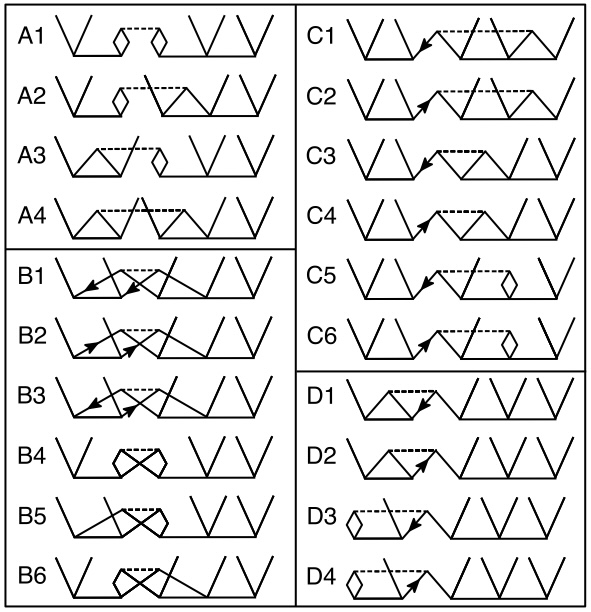
Figure 1: Spin-summed diagrams of $T_{2}T_{3}$ contributions to the triples residuals in CCSDT. For the DC-CCSDT approximation, the diagrams A1 to A4 are kept, B1 to B6 removed and C1 to C6 as well as D1 to D4 multiplied with $0.5$.

II.3 Tensor decompositions

II.3.1 Factorization of electron repulsion integrals

The electron-repulsion integrals (ERIs) are factorized as symmetric contractions of 3 index quantities. In a standard workflow employing explicit basis sets, this is achieved by the density fitting approximation:Baerends, Ellis, and Ros (1973); Whitten (1973); Dunlap, Connolly, and Sabin (1979); Vahtras, Almlöf, and Feyereisen (1993); Feyereisen, Fitzgerald, and Komornicki (1993); Rendell and Lee (1994)

$$v_{pq}^{rs}\approx v_{p}^{rP}\left[v^{-1}\right]_{PQ}v_{q}^{sQ},$$ (7)

where $v_{pq}^{rs}$, $v_{p}^{qP}$ and $v^{PQ}$ are 4-index, 3-index and 2-index ERIs, respectively:

$$v_{pq}^{rs} = \int d\textbf{r}_{1}d\textbf{r}_{2}\frac{\phi^{*}_{p}(\textbf{r}_{1})\phi^{r}(\textbf{r}_{1})\phi^{*}_{q}(\textbf{r}_{2})\phi^{s}(\textbf{r}_{2})}{|\textbf{r}_{1}-\textbf{r}_{2}|},$$ (8)

$$v_{p}^{qP} = \int d\textbf{r}_{1}d\textbf{r}_{2}\frac{\phi^{*}_{p}(\textbf{r}_{1})\phi^{q}(\textbf{r}_{1})\phi^{P}(\textbf{r}_{2})}{|\textbf{r}_{1}-\textbf{r}_{2}|},$$ (9)

$$v^{PQ} = \int d\textbf{r}_{1}d\textbf{r}_{2}\frac{\phi^{P}(\textbf{r}_{1})\phi^{Q}(\textbf{r}_{2})}{|\textbf{r}_{1}-\textbf{r}_{2}|}.$$ (10)

Here the auxiliary orbitals are denoted by capital letter indices $P$, $Q$, while $p$, $q$, $r$ and $s$ denote general (occupied or virtual) spatial orbitals. A symmetric decomposition

$$v_{pq}^{rs}\approx v_{p}^{rL}v_{q}^{sL}$$ (11)

is straightforwardly obtained by

$$v_{p}^{qL}=v_{p}^{qP}\left[v^{-{1\over 2}}\right]_{P}^{L},$$ (12)

where $L$ can correspond to the auxiliary basis functions or to eigenvectors of $v^{PQ}$, etc. Alternatively, the 4-index ERI $v_{pq}^{rs}$ can be obtained in a separate calculation and passed to the ElemCo.jl code via an FCIDUMP-interface (together with the one-electron Hamiltonian).Knowles and Handy (1989) This opens a possibility to apply a high-level correlated treatment to an important orbital subspace only, restricted in the energy or the direct-space representation. Such an approach becomes especially appealing in studying local effects in large moleculesMata, Werner, and Schütz (2008) or periodic systems.Mullan et al. (2022); Christlmaier et al. (2022); R. H. Lavroff (2024) With the 4-index ERIs of the FCIDUMP-interface, density fitting is not applicable. In this case, the factorization in Eq. (11) is performed directly by a diagonalization of the ERI matrix and removal of the eigenvectors corresponding to eigenvalues smaller than a given threshold.

II.3.2 Triples amplitudes decomposition

As is mentioned in the introduction, we employ the decomposition (1) for the triples amplitudes. With the transformation matrices $U$ this decomposition can be also seen as a formal transformation of the triples amplitudes from the SVD basis $T_{XYZ}$ to the orbital basis $T^{ijk}_{abc}$. The transformation connects one index in the SVD space and two indices – one occupied and one virtual – in the orbital space.

In the SVD-DC-CCSDT method the triples amplitudes are varied directly in the SVD basis, such that the residual $R_{XYZ}$ – again in the SVD basis – goes to zero. Importantly, each $U$-transformation can be applied to one SVD index independently of the others. This provides a flexibility, such that the transformation from SVD to the orbital basis in each diagram can be restricted only to the indices that are contracted with the Hamiltonian, while the others can stay in the SVD basis through the complete contraction.

In order to formalize the reduction of the index number and the transformation between the spaces in the SVD-CC theory we introduce new elements in the diagrammatic representation. Firstly it concerns the triples amplitudes $T_{XYZ}$, for which each pair of arrowed particle and hole lines is substituted with an unarrowed SVD line, see Fig. 2a. A transformation of an SVD index in a pair of orbital indices via a $U$ matrix will be denoted by a vertex, an SVD-line below it and a particle and a hole line line above it, see Fig. 2b.

The same principles are applied to the triples residuals that at the end also appear in the SVD basis, which in the diagrammatic representation correspond to the three unarrowed lines, see Fig. 2c. The residuals transform conversely with respect to amplitudes (as covariant and contravariant vectors).Kats, Usvyat, and Schütz (2008) Therefore the transformation $U$ that brings the amplitudes from SVD to the orbital basis, if subjected to transposition and complex conjugation $U^{\dagger}$ , transforms residuals conversely from the orbital basis to SVD. The diagrammatic representation of $U^{\dagger}$ is given in Fig. 2d. $U$ and $U^{\dagger}$ are orthogonal to each other, $U^{\dagger a}_{iX}U^{iY}_{a}=\delta_{X}^{Y}$.

Figure 2: Diagrammatic elements for the SVD-CCSDT formalism: the triples cluster operator in the SVD basis (a), the transformation from the SVD to the orbital basis (b), the residual in SVD basis (c), the transformation from the orbital to the SVD basis (d).

With these rules, we can diagrammatically represent the matrix elements within the SVD-DC-CCSDT formalism. For example Fig. 3 shows two exemplary diagrams from the triples residual: the diagram C6 from Fig. 1 and a triples ladder diagram. The triples amplitudes are given in the SVD basis. Then, as marked by the horizontal blue cuts, for the relevant lines the $U$ transformations to the orbital basis are introduced. After contraction with the Hamiltonian the orbital lines of the residual are transformed back to the SVD basis, as marked by the horizontal red cuts. Finally the vertical green cuts denote the decomposition of the ERIs, Eq. (11).

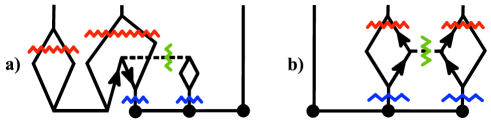
Figure 3: Diagram C6 (a) and a triples-ladder diagram (b) contributing to the triples residuals are shown in the SVD format. The blue wavy lines indicate the insertion of the transformation $U$ (Fig. 2b) from the SVD to the orbital basis, the red wavy lines – of the back transformation $U^{\dagger}$ (Fig. 2d) to the SVD basis. The green wavy lines show the factorization of the ERIs, Eq. (11).

II.4 Residual equations

To achieve an efficient implementation, we obtain the SVD-DC-CCSDT equations in the spin-summed formalism. Given the singlet excitation operator

$$\hat{E}^{a}_{i}=\hat{a}^{\dagger}_{a\alpha}\hat{a}_{i\alpha}+\hat{a}^{\dagger}_{a\beta}\hat{a}_{i\beta}$$ (13)

where the indices $i$ ($j$, $k$, …) and $a$ ($b$, $c$, …) denote the occupied and virtual spatial orbitals, respectively, one defines the standard singly, doubly and triply excited configuration state functions (CSFs):

$$\left|\Phi_{i}^{a}\right> = \hat{E}^{a}_{i}\left|\psi_{0}\right>=\left|\psi^{a}_{i}\right>+\left|\psi^{\bar{a}}_{\bar{i}}\right>$$ (14)

$$\left|\Phi_{ij}^{ab}\right> = {1\over 2}\hat{E}^{a}_{i}\hat{E}^{b}_{j}\left|\psi_{0}\right>$$ (15)

$$= {1\over 2}\left[\left|\psi^{ab}_{ij}\right>+\left|\psi^{\bar{a}\bar{b}}_{\bar{i}\bar{j}}\right>+\left|\psi^{a\bar{b}}_{i\bar{j}}\right>+\left|\psi^{\bar{a}b}_{\bar{i}j}\right>\right],$$

$$\left|\Phi_{ijk}^{abc}\right> = {1\over 6}\hat{E}^{a}_{i}\hat{E}^{b}_{j}\hat{E}^{c}_{k}\left|\psi_{0}\right>$$ (16)

$$= {1\over 6}\left[\left|\psi^{abc}_{ijk}\right>+\left|\psi^{\bar{a}\bar{b}\bar{c}}_{\bar{i}\bar{j}\bar{k}}\right>+\left|\psi^{ab\bar{c}}_{ij\bar{k}}\right>+\left|\psi^{\bar{a}\bar{b}c}_{\bar{i}\bar{j}k}\right>\right.$$

$$+\left.\left|\psi^{a\bar{b}c}_{i\bar{j}k}\right>+\left|\psi^{\bar{a}b\bar{c}}_{\bar{i}j\bar{k}}\right>+\left|\psi^{\bar{a}bc}_{\bar{i}jk}\right>+\left|\psi^{a\bar{b}\bar{c}}_{i\bar{j}\bar{k}}\right>\right]$$

and the corresponding amplitudes

$$\hat{T}_{1} = T^{i}_{a}\hat{E}^{a}_{i},$$ (17)

$$\hat{T}_{2} = {1\over 2}T^{ij}_{ab}\hat{E}^{a}_{i}\hat{E}^{b}_{j},$$ (18)

$$\hat{T}_{3} = {1\over 6}T^{ijk}_{abc}\hat{E}^{a}_{i}\hat{E}^{b}_{j}\hat{E}^{c}_{k}.$$ (19)

The bars on top of the orbital indices indicate the $\beta$-spin.

The singles contributions to the residuals are implemented using the similarity transformation on the Hamiltonian Koch et al. (1996)

$$\tilde{H}_{N}=e^{-\hat{T}_{1}}\hat{H}_{N}e^{\hat{T}_{1}},$$ (20)

which implies “dressing” of the Fock matrices and the ERIs factorization tensors $v_{p}^{qL}$ with the singles amplitudes. The dressed quantities are denoted with a hat.

II.4.1 Singles and doubles residual equations

For the bra-projection in the singles and doubles residual equations we use the contravariant CSFs:Pulay, Saebø, and Meyer (1984); Knowles, Hampel, and Werner (1993)

$$\widetilde{\Phi}_{i}^{a} = \frac{1}{2}\left(\psi_{i}^{a}+\psi_{\bar{i}}^{\bar{a}}\right),$$ (21)

$$\widetilde{\Phi}_{ij}^{ab} = \frac{1}{3}\left(\psi_{ij}^{ab}+\psi_{\bar{i}\bar{j}}^{\bar{a}\bar{b}}+2\psi_{i\bar{j}}^{a\bar{b}}+2\psi_{\bar{i}j}^{\bar{a}b}+\psi_{i\bar{j}}^{b\bar{a}}+\psi_{\bar{i}j}^{\bar{b}a}\right).$$ (22)

The pure singles and doubles terms with such a bra-projection can be found in the ElemCo.jl documentation.ele Here we focus only on the terms that involve the triples. To get the actual expressions for these terms within the SVD-DC-CCSDT we adopt the following protocol:

1. Calculate the algebraic expressions for the matrix element at question with the program Quantwo,Kats and Schraivogel (2023) which symbolically evaluates all the terms for the given bra- and ket-CSFs using the Wick’s theorem.

2. Replace the triples amplitudes with the SVD-decomposed form, Eq. (1), and the ERIs with the factorized form, Eq. (11).

3. Factorize the equations. For this the diagrammatic representation can be used, as discussed in section II.3.2 (see Figs 2 and 3).

After introducing intermediates, this yields for triples contributions to the singles residual:

$$R_{a}^{i} \leftarrow U_{a}^{iX}\left[T_{XYZ}\left(2A^{LY}A^{LZ}-{B}_{j}^{kLZ}{B}_{k}^{jLY}\right)\right]$$ (23)

$$-U_{a}^{jY}\Big{[}2{B}_{j}^{iLX}\left(T_{XYZ}A^{LZ}\right)$$

$$\,\,\,\,-T_{XYZ}\left(U_{d}^{iX}\left(\left(v_{j}^{cL}v_{k}^{dL}\right)U_{c}^{kZ}\right)\right)\Big{]},$$

with intermediates

$$A^{LX} = {B}_{i}^{iLX},\hskip 28.45274pt{B}_{i}^{jLX}=v_{i}^{aL}U_{a}^{jX}.$$ (24)

The parentheses denote the contraction order. The triples contributions to the doubles residual read:

$$R_{ab}^{ij} \leftarrow \mathcal{S}\left(ij,ab\right)\Big{\{}U_{a}^{iX}\Big{[}U_{b}^{jY}\left(T_{XYZ}\left(\hat{f}_{k}^{c}U_{c}^{kZ}\right)\right)$$

$$-\left(T_{XYZ}U_{b}^{kZ}\right)\left(\hat{f}_{k}^{c}U_{c}^{jY}\right)\Big{]}$$

$$+2U_{b}^{jY}\Big{[}\left(\bar{B}_{a}^{iLZ}-B_{a}^{iLZ}\right)\left(T_{XYZ}A^{LX}\right)\Big{]}$$

$$+\left(B_{a}^{iLZ}-\bar{B}_{a}^{iLZ}\right)\left({B}_{k}^{jLY}\left(T_{XYZ}U_{b}^{kX}\right)\right)$$

$$-U_{b}^{jZ}\left(T_{XYZ}\left(U_{c}^{iY}\left(\bar{B}_{a}^{kLX}v_{k}^{cL}\right)-U_{a}^{kY}\left(B_{c}^{iLX}v_{k}^{cL}\right)\right)\right)\Big{\}},$$

with intermediates

$$B_{a}^{iLX}=\hat{v}_{j}^{iL}U_{a}^{jX},\hskip 28.45274pt\bar{B}_{a}^{iLX}=\hat{v}_{a}^{bL}U_{b}^{iX},$$ (26)

and the symmetrization operator

$$\mathcal{S}\left(ij,ab\right)X_{ab}^{ij}=X_{ab}^{ij}+X_{ba}^{ji}.$$ (27)

The correlation energy $E$ is calculated as usually using the singles and doubles amplitudes:

$$E = \left(2T_{a}^{i}T_{b}^{j}-T_{b}^{i}T_{a}^{j}\right)v_{ij}^{ab}+2T_{a}^{i}f^{a}_{i}$$ (28)

$$+(2T_{ab}^{ij}-T_{ba}^{ij})v_{ij}^{ab}.$$

II.4.2 Triples residual equations

For the triply excited covariant CSF the permutation of virtual orbital indices leads to a linear dependency for one CSF on the other five CSFs.Schütz (2000); Paldus and Jeziorski (1988) As a result a fully orthogonal contravariant CSF for the bra-projection cannot be constructed for triples. We employ the contravariant triples CSFs of Ref. Schütz, 2000 (apart from the 1/6 prefactor, which in our case is absorbed in the covariant CSF $\Phi_{ijk}^{abc}$, eq. (16)). To ease the evaluation of the matrix elements with the Quantwo programKats and Schraivogel (2023) we express it via the covariant ones as

$$\widetilde{\Phi}_{abc}^{ijk}={\Phi}_{abc}^{ijk}-{\Phi}_{cab}^{ijk}.$$ (29)

Importantly, due to the overlap properties of the chosen contravariant and covariant CSFs (see eq. (8) of Ref. Schütz, 2000)

$$\left<\widetilde{\Phi}_{abc}^{ijk}|{\Phi}^{abc}_{ijk}\right> = 1$$

$$\left<\widetilde{\Phi}_{abc}^{ijk}|{\Phi}^{acb}_{ijk}\right> = \left<\widetilde{\Phi}_{abc}^{ijk}|{\Phi}^{bac}_{ijk}\right>=\left<\widetilde{\Phi}_{abc}^{ijk}|{\Phi}^{bca}_{ijk}\right>=\left<\widetilde{\Phi}_{abc}^{ijk}|{\Phi}^{cba}_{ijk}\right>$$

$$= 0$$

$$\left<\widetilde{\Phi}_{abc}^{ijk}|{\Phi}^{cab}_{ijk}\right> = -1$$ (30)

the matrix elements with such a contravariant CSF bra-projection will consist of two sets of terms. The second set can be obtained from the first one by the index-permutation $abc\rightarrow cab$ and multiplication with -1. This can be expressed by the antisymmetrized permutation operator

$$\mathcal{P}(abc;cab)F(a,b,c) = F(a,b,c)-F(c,a,b)$$ (31)

For an illustration, consider a simple matrix element $\left<\widetilde{\Phi}_{abc}^{ijk}|\hat{T}_{3}|\psi_{0}\right>$. Due to the overlap relations (30)

$$\left<\widetilde{\Phi}_{abc}^{ijk}|\hat{T}_{3}|\psi_{0}\right>=T^{ijk}_{abc}-T^{ijk}_{cab}=\mathcal{P}(abc;cab)T^{ijk}_{abc}.$$ (32)

For this effect in the (T) residual we refer to eq. (17) in Ref. Schütz, 2000. Similarly, the full CCSDT triples residual $\bar{R}^{ijk}_{abc}$ can be represented by two terms $R^{ijk}_{abc}$ and $R^{ijk}_{cab}$, one obtained by an index permutation of the other:

$$\left<\tilde{\Phi}_{abc}^{ijk}|\exp\left(-\hat{T}_{2}-\hat{T}_{3}\right)\tilde{H}_{N}\exp\left(\hat{T}_{2}+\hat{T}_{3}\right)|\psi_{0}\right>=\bar{R}^{ijk}_{abc}$$

$$\,\,\,\,\,\,\,\,\,\,\,\,\,\,\,\,\,\,=R^{ijk}_{abc}-R^{ijk}_{cab}=\mathcal{P}(abc;cab)R^{ijk}_{abc}$$ (33)

Importantly, when the $R^{ijk}_{abc}$ residual vector is zero the permuted term $R^{ijk}_{cab}$ is zero too. Therefore it is sufficient to solve the equations:

$$R^{ijk}_{abc}=0$$ (34)

with just half of the terms of the initial residual $\bar{R}^{ijk}_{abc}$.

To define the triples residual equations to be solved we introduce a formal operator $\mathcal{P}^{-1}(abc;cab)$ as an inverse of the initial operator

$$\mathcal{P}^{-1}(abc;cab)\mathcal{P}(abc;cab)=1.$$ (35)

It has an obvious property:

$$\mathcal{P}^{-1}(abc;cab)\left[F(a,b,c)-F(c,a,b)\right]=F(a,b,c).$$ (36)

With this operator we can define our bra-projection for the triples residual equations as $\mathcal{P}^{-1}(abc;cab)\left<\tilde{\Phi}_{abc}^{ijk}\right|$, where the operator $\mathcal{P}^{-1}(abc;cab)$ is meant to be applied not to the bra-function only but rather to the complete matrix element. With that we obtain

$$\mathcal{P}^{-1}(abc;cab)\left<\tilde{\Phi}_{abc}^{ijk}\right|$$

$$\,\,\,\,\,\,\,\,\,\,\,\,\,\,\,\,\,\left.\exp\left(-\hat{T}_{2}-\hat{T}_{3}\right)\tilde{H}_{N}\exp\left(\hat{T}_{2}+\hat{T}_{3}\right)|\psi_{0}\right>=R^{ijk}_{abc}.$$ (37)

Technically, application of the operator $\mathcal{P}^{-1}(abc;cab)$ to a set of terms, obtained by expanding the matrix element, involves a polynomial division of these terms by $\mathcal{P}(abc;cab)$, represented as a linear of combination of virtual index permutations: $(123)-(312)$.

Below we summarize the workflow for the determination of the terms in the triples residual equations of SVD-DC-CCSDT.

1. Calculate the algebraic expressions for the matrix element $\left<\tilde{\Phi}_{abc}^{ijk}|\exp\left(-\hat{T}_{2}-\hat{T}_{3}\right)\tilde{H}_{N}\exp\left(\hat{T}_{2}+\hat{T}_{3}\right)|\psi_{0}\right>$ using the program Quantwo.Kats and Schraivogel (2023)

2. Apply the operator $\mathcal{P}^{-1}(abc;cab)$ to the obtained terms using Quantwo.

3. Identify the B-, C- and D-diagrams of Fig. 1 and scale or remove them to define the DC-CCSDT approximation. It can also be done in Quantwo by subtracting the corresponding terms.

4. Replace the triples amplitudes with the SVD-decomposed form, Eq. (1), the ERIs with the factorized form, Eq. (11), and multiply the residual equation with $U^{\dagger a}_{iX}U^{\dagger b}_{jY}U^{\dagger c}_{kZ}$.

5. Factorize the terms considering the orthogonality of $U$ using common intermediates. The latter can be identified by searching for identical diagrammatic fragments after slicing the diagrams according to Fig. 3.

The triples residual equations in the SVD basis, obtained using this protocol, read:

$$R_{XYZ} = Q_{XYZ}+Q_{YXZ}+Q_{XZY}+Q_{ZYX}+Q_{ZXY}+Q_{YZX}$$ (38)

$$+q_{XYZ}+q_{YXZ}+q_{ZYX}$$

with the main intermediates

$$Q_{XYZ} = U^{\dagger b}_{jY}\Big{[}T_{bX}^{l}X_{lZ}^{j}-X_{bZ}^{d}T_{dX}^{j}$$ (39)

$$+\left(T_{X^{\prime}Y^{\prime}Z}U_{b}^{lX^{\prime}}\right)\left(U_{d}^{jY^{\prime}}\left(v_{l}^{dL}Y_{X}^{L}\right)\right)\Big{]}$$

and

$$q_{XYZ} = T_{X^{\prime}YZ}\Big{[}U_{a}^{lX^{\prime}}\left(\left(\hat{f}_{l}^{i}+0.5v_{l}^{dL}V_{d}^{iL}\right)U^{\dagger a}_{iX}\right)$$ (40)

$$-U^{\dagger a}_{iX}\left(\left(\hat{f}_{a}^{d}-0.5v_{l}^{dL}V_{a}^{lL}\right)U_{d}^{iX^{\prime}}\right)$$

$$+U^{\dagger a}_{iX}\left(\left(\hat{v}_{l}^{iL}\hat{v}_{a}^{dL}\right)U_{d}^{lX^{\prime}}\right)-2Y_{X}^{L}A^{LX^{\prime}}\Big{]}$$

$$-T_{XY^{\prime}Z^{\prime}}\left(W_{Y}^{Y^{\prime}L}W_{Z}^{Z^{\prime}L}\right).$$

The further intermediates used in these expressions are

$$X_{bZ}^{d} = \hat{v}_{b}^{dL}Y_{Z}^{L}-\hat{f}_{l}^{d}T_{bZ}^{l}+v_{l}^{dL}\Big{[}G_{bZ}^{lL}-\hat{v}_{b}^{cL}T_{cZ}^{l}\Big{]}$$

$$+0.5T_{X^{\prime}Y^{\prime}Z}\left(U_{b}^{kY^{\prime}}w_{k}^{dX^{\prime}}\right),$$

$$X_{lZ}^{j} = \hat{v}_{l}^{jL}Y_{Z}^{L}-v_{l}^{dL}\Big{[}G_{dZ}^{jL}+\hat{v}_{k}^{jL}T_{dZ}^{k}\Big{]}$$ (41)

$$-0.5T_{X^{\prime}Y^{\prime}Z}\left(U_{d}^{jY^{\prime}}w_{l}^{dX^{\prime}}\right)$$

and

$$\begin{split}&G_{bX}^{jL}=T_{bc}^{jk}\left(U^{\dagger c}_{lX}\hat{v}_{k}^{lL}-U_{kX}^{\dagger d}\hat{v}_{d}^{cL}\right)-U_{b}^{jZ^{\prime}}\Big{[}T_{XY^{\prime}Z^{\prime}}A^{LY^{\prime}}\\ &\qquad-0.5\left(\left(U_{c}^{mX^{\prime}}T_{X^{\prime}Y^{\prime}Z^{\prime}}\right)B_{m}^{kLY^{\prime}}\right)U^{\dagger c}_{kX}\Big{]}\end{split}$$ (42)

$$\begin{split}&V_{a}^{iL}=v_{k}^{cL}\widetilde{T}_{ac}^{ik}\hskip 42.67912ptY_{X}^{L}=U^{\dagger a}_{iX}\left(\hat{v}_{a}^{iL}+V_{a}^{iL}\right)\\ &T_{aX}^{i}=U^{\dagger b}_{jX}T_{ab}^{ij}\hskip 36.98866pt\widetilde{T}_{ab}^{ij}=2T_{ab}^{ij}-T_{ba}^{ij}\\ &w_{k}^{dX}=v_{l}^{dL}{B}_{k}^{lLX}\hskip 31.2982ptW_{Y}^{Y^{\prime}L}=U^{\dagger b}_{jY}\left(B_{b}^{jLY^{\prime}}-\bar{B}_{b}^{jLY^{\prime}}\right).\end{split}$$ (43)

None of the contractions in eqs. (23)-(26) and (39)-(43) involve more than six different indices. This means that the tensor decompositions reduce the scaling of the DC-CCSDT method, which conventionally is ${\cal O}(N^{8})$, to ${\cal O}(N^{6})$, provided the number of SVD basis functions grows linearly with the system size (vide infra). Furthermore, some particularly nasty terms become inexpensive, like e.g. the 4-external ladder diagram of the triples amplitudes (the term in the sixth line of eq. (40)), which is reduced to even $N^{5}$.

The most expensive terms in the triples residual equations scale as $N_{o}^{2}N_{v}N_{X}^{2}N_{L}$, where $N_{o}$ and $N_{v}$ are the numbers of occupied and virtual orbitals, and $N_{X}$ and $N_{L}$ are the numbers of SVD and density-fitting basis functions, respectively. Assuming $N_{v}\approx N_{X}$ (vide infra), the most expensive terms in SVD-DC-CCSDT are only a factor of $N_{L}/N_{v}$ more expensive than the most expensive term in CCSD (the 4-external ladder diagram with the $N_{o}^{2}N_{v}^{4}$ scaling). This is a significant improvement over the SVD-CCSDT method (especially for large basis sets), where the most expensive term scales as $N_{o}N_{v}^{2}N_{X}^{3}$, see Ref. Lesiuk, 2020. Note that it is possible to further reduce the scaling of the iterative solution of the triples residual equations by using a different factorization of the $G$ intermediate in eq. (42), such that the $N_{o}^{2}N_{v}N_{X}^{2}N_{L}$-scaling terms become independent of the amplitudes and have to be computed only once and can be reused in each iteration.

II.5 Construction of the SVD basis

In order to achieve the ${\cal O}(N^{6})$ scaling of the SVD-DC-CCSDT method at every stage of the calculation, the construction of the singular vectors $U^{iX}_{a}$ should scale not higher than that. Generally the singular values and singular vectors can be obtained by diagonalizing an approximate triples two-particle density matrix block $D^{aj}_{ib}$. This diagonalization scales as $N^{6}$, but the computation of such density matrix scales as $N^{8}$ even at the (T)-level. To reduce this scaling we use a two-step procedure.

First, we obtain the relevant block of the approximate two-particle density matrix from converged CCSD doubles amplitudes

$$\mathcal{D}^{aj}_{ib}=T^{\dagger ac}_{ik}T^{jk}_{bc},$$ (44)

and eigendecompose it,

$$\mathcal{D}^{aj}_{ib}\approx\bar{U}_{i\tilde{\bar{X}}}^{\dagger a}\bar{D}_{\tilde{\bar{X}}}\bar{U}^{j\tilde{\bar{X}}}_{b}.$$ (45)

In the decomposition (45) the SVD basis $\{\tilde{\bar{X}}\}$ is truncated by disregarding the eigenvectors that correspond to eigenvalues smaller than a threshold: $\bar{D}_{\tilde{\bar{X}}}<\varepsilon_{T2}$.

Next, triples amplitudes in the mixed – orbital and doubles-SVD – basis are computed. For this purpose we canonicalize the latter by diagonalizing the Fock matrix in the SVD basis $f_{\tilde{\bar{X}}}^{\tilde{\bar{Y}}}$:

$$f_{\tilde{\bar{X}}}^{\tilde{\bar{Y}}}=\bar{U}_{i\tilde{\bar{X}}}^{\dagger a}(\epsilon_{a}-\epsilon_{i})\bar{U}^{i\tilde{\bar{Y}}}_{a}.$$ (46)

In the basis of its eigenvectors $U_{\tilde{\bar{X}}}^{\bar{X}}$ the Fock matrix (46) is diagonal

$$f^{{\bar{X}}}_{{\bar{Y}}}=\epsilon_{\bar{X}}\delta^{{\bar{X}}}_{{\bar{Y}}}$$ (47)

and the complete transformation to the ${\bar{X}}$-basis is given by

$$\bar{U}^{i{\bar{X}}}_{a}=\bar{U}^{i\tilde{\bar{X}}}_{a}\bar{U}_{\tilde{\bar{X}}}^{\bar{X}}.$$ (48)

Having the transformation matrices to the (doubles) SVD-basis at hand we can obtain a partially decomposed CC3-type triples residual

$$R^{i}_{a\bar{X}\bar{Y}} = \left(\left(T^{j}_{c\bar{X}}v^{cL}_{b}\right)\bar{U}^{\dagger b}_{j\bar{Y}}\right)\hat{v}_{a}^{iL}-V^{i}_{l\bar{X}}T^{l}_{a\bar{Y}}+E^{d}_{l\bar{X}\bar{Y}}T_{ad}^{il}$$ (49)

$$-\left(\left(T^{l}_{b\bar{X}}\hat{v}^{jL}_{l}\right)\bar{U}^{\dagger b}_{j\bar{Y}}\right)\hat{v}_{a}^{iL}+V_{a\bar{X}}^{d}T^{i}_{d\bar{Y}}$$

with the intermediates

$$\begin{split}&E^{d}_{l\bar{X}\bar{Y}}=V_{a\bar{X}}^{d}\bar{U}_{l\bar{Y}}^{\dagger a}-V_{l\bar{X}}^{i}\bar{U}_{i\bar{Y}}^{\dagger d}\\ &V^{d}_{a\bar{X}}=\hat{v}_{a}^{dL}W^{L}_{\bar{X}}\hskip 56.9055ptV^{j}_{l\bar{X}}=\hat{v}^{jL}_{l}W^{L}_{\bar{X}}\\ &T_{a\bar{X}}^{i}=\bar{U}^{\dagger b}_{j\bar{X}}T^{ij}_{ab}\hskip 56.9055ptW_{\bar{X}}^{L}=\hat{v}_{c}^{kL}\bar{U}^{\dagger c}_{k\bar{X}}\\ \end{split}$$ (50)

at the $N^{6}$ cost at most. This scaling corresponds to the third term of eq. (49), while all other terms scale even as $N^{5}$. Since the SVD basis is canonicalized, the partially transformed triples amplitudes are readily available:

$$T^{i}_{a\bar{X}\bar{Y}} = \;-\frac{R^{i}_{a\bar{X}\bar{Y}}+R^{i}_{a\bar{Y}\bar{X}}}{(\epsilon_{\bar{X}}+\epsilon_{\bar{Y}}+\epsilon_{a}-\epsilon_{i})}$$ (51)

and with that – the triples two-particle density matrix

$$D^{aj}_{ib} = T^{\dagger a\bar{X}\bar{Y}}_{i}T_{b\bar{X}\bar{Y}}^{j}$$ (52)

again at the $N^{6}$ cost.

In the SVD basis the triples amplitudes implicitly include nonphysical components with triply repeated occupied orbital indices like $T_{abc}^{iii}$ which would cancel in case of a full SVD basis. However, it is possible to explicitly isolate and discard their contributions to the density matrix:

$$\Delta D^{aj}_{ib}=(T^{\dagger a}_{i\bar{X}\bar{Y}}\mathcal{U}^{\bar{X}}_{i\bar{X}^{\prime}}\mathcal{U}^{\bar{Y}}_{i\bar{Y}^{\prime}})T^{j\bar{X}^{\prime}\bar{Y}^{\prime}}_{b}$$ (53)

with

$$\mathcal{U}^{\bar{X}}_{i\bar{X}^{\prime}}=\sum_{a}\bar{U}^{\dagger a}_{i\bar{X}^{\prime}}\bar{U}^{i\bar{X}}_{a}$$ (54)

such that

$$\widetilde{D}^{aj}_{ib} = D^{aj}_{ib}-\left(1-\frac{1}{2}\delta^{i}_{j}\right)\mathcal{S}(ij,ab)\Delta D^{aj}_{ib}.$$ (55)

Finally we obtain the actual SVD basis for the triples in DC-CCSDT by diagonalizing the triples two-electron density matrix $\widetilde{D}^{aj}_{ib}$

$$\widetilde{D}^{aj}_{ib}\approx U^{\dagger a}_{i\tilde{X}}D_{\tilde{X}}U^{j\tilde{X}}_{b}.$$ (56)

Analogously to the doubles SVD, we disregard all the vectors whose eigenvalues are smaller than the chosen threshold: $D_{\tilde{X}}<\varepsilon_{T3}$. Again, before the use in DC-CCSDT the SVD-basis is canonicalized by diagonalizing the Fock matrix

$$f_{\tilde{X}}^{\tilde{Y}}=U_{i\tilde{X}}^{\dagger a}(\epsilon_{a}-\epsilon_{i})U^{i\tilde{Y}}_{a}.$$ (57)

The eigenvectors $U_{\tilde{X}}^{X}$ of $f_{\tilde{X}}^{\tilde{Y}}$ are used in the final SVD transformation matrices

$$U^{iX}_{a}=U^{i\tilde{X}}_{a}\bar{U}_{\tilde{X}}^{X}.$$ (58)

The matrices $U^{iX}_{a}$ of eq. (58) are the ones that are used in the DC-CCSDT residual equations given in section II.4.

The eigenvalues $\epsilon_{X}$ of $f_{\tilde{X}}^{\tilde{Y}}$ are employed in the update, which is carried out directly in the SVD basis:

$$\Delta T_{XYZ}=-\frac{R_{XYZ}}{\epsilon_{X}+\epsilon_{Y}+\epsilon_{Z}}.$$ (59)

Due to the symmetry property $T_{XYZ}=T_{YXZ}=T_{XZY}=T_{ZYX}=T_{ZXY}=T_{YZX}$ one can restrict solving the residual equations to $X\leq Y\leq Z$. However, since our implementation is based on the implicit tensor contraction library TensorOperations.jlLukas Devos <lukas.devos@ugent.be> and contributors (2023) we keep the full tensors. To accelerate the convergence of DC-CCSDT we employ the direct inversion of the iterative subspace (DIIS) for singles, doubles and triples amplitude vectors.

III Test Calculations

To test the performance of SVD-DC-CCSDT we benchmark it against DC-CCSDT and CCSDT(Q) for a set of reaction energies from Ref. Huntington et al., 2012. Below we focus on the mean absolute (MEAN), the root mean square (RMS) and the maximum (MAX) deviations for the complete set. The detailed compilation of the results for each individual reaction can be found in the supplementary material.

All CCSD(T), DC-CCSDT, SVD-CCSD(T) and SVD-DC-CCSDT calculations are performed using ElemCo.jlKats et al. (2024), a Julia-based quantum chemistry package. ElemCo.jl includes an interface to the libcintSun (2015) library for the electron-repulsion integrals. In the calculations we use the orbital basis sets from the Dunning basis set family.Dunning Jr (1989) In the post-HF treatment the core is not correlated, and the density fitting approximation employs the respective auxiliary basis sets.Weigend, Köhn, and Hättig (2002) In the density fitted HF the def2-universal-jkfit auxiliary basis setWeigend (2008) is chosen.

Firstly, we investigate the effect of the truncation of the SVD basis for the CCSD doubles amplitudes, eq. (45), used to calculate the triples density matrix for the subsequent decomposition of the triples. This truncation, governed by the threshold $\varepsilon_{T2}$, is an additional approximation to the SVD-DC-CCSDT method. Therefore it is important to keep its influence negligible compared to that of the truncation of the SVD-basis for the triples. In order to guarantee that by tightening of the triples SVD threshold $\varepsilon_{T3}$ the threshold $\varepsilon_{T2}$ would automatically be tightened too, we link the two by a factor $w_{T2}$:

$$\varepsilon_{T2}=w_{T2}\varepsilon_{T3}.$$ (60)

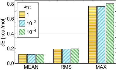
Figure 4: The mean, RMS and maximum deviations of the SVD-DC-CCSDT reaction energies as functions of the $w_{T2}$ weight factor for the $\varepsilon_{T2}$ tolerance (see eq. (60)) with respect to the CCSDT(Q) reference. The calculations employ the cc-pVDZ basis and fixed $\varepsilon_{T3}=10^{-6}$.

Fig. 4 presents the deviations of the SVD-DC-CCSDT energies from the CCSDT(Q) reference calculated with different values of $w_{T2}$ – from 10^-4 to 1. Surprisingly, the accuracy of the method is insensitive to the choice of $w_{T2}$. A likely reason of such a minute effect of the truncation of the SVD-basis for the doubles is only a partial representation of the triples residuals (49) and the corresponding triples amplitudes (51) in the truncated SVD basis. Therefore, the two-particle density matrix (52) still contains information about the complete orbital space.

Next, we focus on the main approximation of the method – the truncation of the triples SVD space. In Fig. 5a it is demonstrated that the SVD-DC-CCSDT reaction energies for the test set calculated with the cc-pVDZ basis, progressively approach the untruncated DC-CCSDT ones with tightening of the threshold $\varepsilon_{T3}$. The appreciable accuracy (the mean and RMS deviations $<0.1$ kcal/mol, maximum deviation $~{}0.2$ kcal/mol), however, can only be achieved with $\varepsilon_{T3}$ not higher than 10^-6. A comparison to the higher-level CCSDT(Q) results, shown in Fig. 5b reveals that at this value of $\varepsilon_{T3}$ the truncation error becomes smaller than the DC-CCSDT method error.

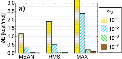
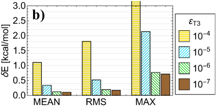
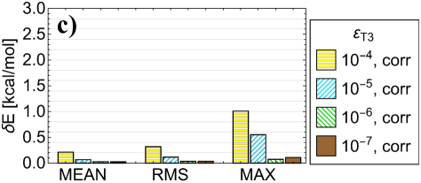
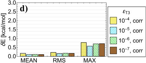
Figure 5: The mean, RMS and maximum deviations of the SVD-DC-CCSDT reaction energies as functions of the $\varepsilon_{T3}$ tolerance with respect to the DC-CCSDT (panels a and c) and CCSDT(Q) (panels b and d) references. The calculations employ the cc-pVDZ basis and fixed $w_{T2}=10^{-2}$. In panels c and d, the SVD error was corrected using the hybrid approach of eqs. (61) and (62).

In order to accelerate convergence with the SVD truncation threshold we tested a hybrid approach with the SVD-error correction at the CCSD(T) level:

$$E_{\textrm{DC-CCSDT}}\approx E_{\textrm{SVD-DC-CCSDT}}+\delta_{\rm SVD}$$ (61)

with

$$\delta_{\rm SVD}=E_{\textrm{CCSD(T)}}-E_{\textrm{SVD-CCSD(T)}}.$$ (62)

As is seen in Fig. 5c, the hybrid approach (61) indeed converges noticeably faster. A sufficient accuracy is achieved already with $\varepsilon_{T3}=10^{-5}$. Interestingly, comparison to CCSDT(Q) in Fig. 5d shows that the SVD-error in the hybrid scheme is no longer dominant even for $\varepsilon_{T3}=10^{-4}$.

A qualitatively similar picture is observed for larger basis sets – aug-cc-pVDZ and cc-pVTZ – shown in Fig. 6. Due to the computational cost, for these basis sets not only the CCSDT(Q) reference is unfeasible but also the untruncated DC-CCSDT one. So here we use the SVD-DC-CCSDT results with $\varepsilon_{T3}=10^{-6}$ obtained with the hybrid scheme (61) as the reference. Again the pure SVD-DC-CCSDT is reliable provided the threshold $\varepsilon_{T3}$ is tightened to 10^-6. With the hybrid approach, however, a comparable accuracy is reached already with $\varepsilon_{T3}=10^{-5}$. Moreover, even with a very crude tolerance of $\varepsilon_{T3}=10^{-4}$ the RMS and mean deviations of the hybrid scheme are about 0.2 kcal/mol and the maximum deviation for the reaction set is smaller than 1 kcal/mol.

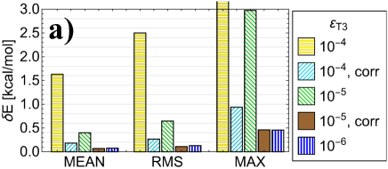
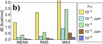
Figure 6: The mean, RMS and maximum deviations of the SVD-DC-CCSDT reaction energies as functions of the $\varepsilon_{T3}$ tolerance, calculated with and without the hybrid approach (see eqs. (61) and (62)) and two different basis sets: aug-cc-pVDZ (panel a) and cc-pVTZ (panel b). The reference results were obtained with the hybrid approach and $\varepsilon_{T3}=10^{-6}$. In all the calculations the weight $w_{T2}$ of $10^{-2}$ was chosen.

A possibility to use looser $\varepsilon_{T3}$ thresholds, provided by the hybrid approach, is essential, as it has a strong impact on the computational cost. In table 1 we list the sizes of the SVD space and timings of the SVD-DC-CCSDT calculations (within the hybrid scheme) on a benzene molecule with different basis sets. Tightening of $\varepsilon_{T3}$ by an order of magnitude results in an increase of the time for a SVD-DC-CCSDT iteration also by an order of magnitude on average. Furthermore, for the threshold values of 10^-4 or 10^-5 the cost of the SVD-DC-CCSDT calculations is lower or comparable to that of the untruncated (T) needed for the hybrid scheme (61). Interestingly, the size of the SVD basis after truncation within a given threshold does grow with the orbitals basis but very slowly, much slower than the number of virtual orbitals.

Table 1: The number of the SVD basis functions ($n_{\textrm{SVD}}$) and respective timings (per iteration $t_{\textrm{ITER}}$ and total $t_{\textrm{TOTAL}}$ for SVD-DC-CCSDT calculations on the benzene molecule from the test set with with different $\varepsilon_{T3}$ thresholds and cc-pVDZ, aug-cc-pVDZ and cc-pVTZ basis sets. The number of virtual orbitals for each basis set is denoted by $n_{\textrm{virt}}$. The weight $w_{T2}=10^{-2}$ was chosen. All calculations were performed on 12-core Intel Xeon Gold 6128 nodes with the rate of 3.40GHz.

	$\varepsilon_{T3}$	$n_{\textrm{SVD}}$	$t_{\textrm{ITER}}\textrm{[min]}$	$t_{\textrm{TOTAL}}\textrm{[h]}$
cc-pVDZ	$10^{-4}$	33	0.13	0.17
($n_{\textrm{virt}}=93$)	$10^{-5}$	147	1.21	0.42
	$10^{-6}$	440	26.29	5.60
	$10^{-7}$	950	382.21	76.70
aug-cc-pVDZ	$10^{-4}$	36	0.46	1.63
($n_{\textrm{virt}}=171$)	$10^{-5}$	161	3.17	2.18
	$10^{-6}$	494	70.14	13.58
cc-pVTZ	$10^{-4}$	36	0.82	6.97
($n_{\textrm{virt}}=243$)	$10^{-5}$	187	5.62	8.13
	$10^{-6}$	592	111.91	30.14

Finally we investigate how the size of the truncated SVD basis and the truncation error scale with the system size. The theoretical $N^{6}$ scaling that formally follows from the equations (38)-(43) and (49)-(52) will be reproduced in practice only if the number of the SVD-basis functions after truncation grows linearly with systems size. Furthermore, for the size-extensivity of the method it is vital that the SVD-truncation error also scales linearly with the systems size. In order to test these two aspects we considered a set of formal linear alkanes from $(\textrm{CH}_{2})_{2}\textrm{H}_{2}$ to $(\textrm{CH}_{2})_{5}\textrm{H}_{2}$ with the following parameters: $r_{\textrm{C-C}}=1.54$ Å, $r_{\textrm{C-H}}=1.1$ Å and $\alpha_{\textrm{C-C-C}}=\alpha_{\textrm{H-C-H}}=109.5^{\circ}$.

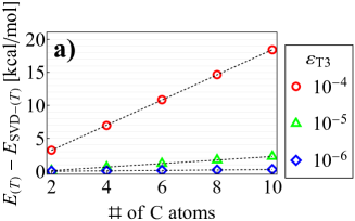
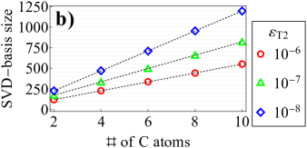
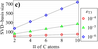
Figure 7: The SVD-error of the SVD-(T) energy (panel a) and the SVD basis sizes as functions of the length of linear alkane chains from $(\textrm{CH}_{2})_{2}\textrm{H}_{2}$ to $(\textrm{CH}_{2})_{5}\textrm{H}_{2}$, calculated with different thresholds $\varepsilon_{T3}$. Panel b reports the sizes of the SVD-space for the doubles decomposition (see eqs. (45)-(52)), the panel c – the SVD space for the triples decomposition.

Firstly, we focus on the size-extensivity of the SVD truncation error. Since the DC-CCSDT calculations for larger alkanes are too expensive, we evaluate this error at the SVD-(T) level. As is seen from Fig. 7a the error is clearly linear with the system size for all the thresholds used, confirming the size-extensivity of the truncation strategy based on the cutoff tolerance. As concerns the error itself, with $\varepsilon_{T3}=10^{-4}$ it is clearly unacceptably large. With $\varepsilon_{T3}=10^{-6}$ the errors are very small: for the largest alkane considered, the error in the total (T) energy is below 0.3 kcal/mol. The choice $\varepsilon_{T3}=10^{-5}$ leads to small errors, but not necessarily negligible for larger systems. However, as established above, the hybrid scheme reduces this error to appreciable levels. Finally, the linear growth of the truncated SVD-spaces is also reproduced, as is evident from Figs. 7b and 7c.

IV Conclusions

In this work we presented an SVD-DC-CCSDT method, which is a very accurate but much less expensive approximation to DC-CCSDT. In SVD-DC-CCSDT the triples amplitudes as well as the triples residuals are represented in the truncated basis of singular vectors. At no point in the method the full triples amplitudes in the molecular orbital basis need to be processed. The factorization of the intermediates in the triples residual equations achieved by the decomposition of the triples amplitudes and the density fitting reduces the scaling from ${\cal O}(N^{8})$ to ${\cal O}(N^{6})$. The DC approximation not only improves the accuracy of the CCSDT method, but also removes the most expensive terms from the SVD-CCSDT method.

The determination of the SVD transformation matrices is evaluated via the CC3-like triples contribution to the 2-particle density matrix. This procedure also scales as ${\cal O}(N^{6})$ due to a partial transformation of the involved intermediates in an auxiliary SVD basis for the doubles amplitudes.

The truncation of both SVD spaces are governed by the tolerances $\varepsilon_{T3}$ for the triples and $\varepsilon_{T2}$ in the auxiliary SVD for the doubles. These thresholds are compared to the eigenvalues of the respective two-electron density matrices. The choice of $\varepsilon_{T2}$ has a very little effect on the results, at least if it is not larger than $\varepsilon_{T3}$. At the same time, the SVD-error depends on the choice $\varepsilon_{T3}$ itself quite strongly. By benchmarking reaction energies for a test set of 42 small molecules, it was determined that with the $\varepsilon_{T3}=10^{-6}$ the error of the SVD approximation is smaller than the error of the DC-CCSDT method itself compared to CCSDT(Q). A correction of the SVD error at the SVD-(T) level allows one to loosen this tolerance to $10^{-5}$. Regardless of the choice of $\varepsilon_{T3}$, the SVD error in the energy and the size of the SVD bases scale linearly with the system size.