Cold Quark Matter: Renormalization Group improvement
at next-to-next-to leading order

Abstract

We extend previous next-to-next-to leading order (NNLO) calculations of the QCD pressure at zero temperature and non-zero baryonic densities using the renormalization group optimized perturbation theory (RGOPT), which entails an all-order RG-invariant resummation. First, we consider the approximation of three massless quark flavors, and then adding the running strange quark mass dependence. The resulting pressure displays a sizeably reduced sensitivity to variations of the arbitrary renormalization scale as compared to the state-of-the-art NNLO results. This confirms previous NLO investigations that the RGOPT resummation scheme provides improved convergence properties and reduced renormalization scale uncertainties, thus being a promising prescription to improve perturbative QCD at high and mid range baryonic densities.

I Introduction

Quantum Chromodynamics (QCD) displays nonperturbative features, even at weak coupling values, when either finite temperature ($T$) and/or baryonic density are taken in consideration. This complication is due to the apparition of long-range correlations in the medium for the gluonic fields (see Trev for reviews), making any analytical approaches to the determination of the partition function and associated thermodynamical quantities challenging. For vanishing baryonic densities and high temperatures, the state-of-the-art thermodynamical calculationslattice are held by lattice QCD (LQCD) simulations, however, owing to the sign problem in the fermionic sectorsign , presently LQCD cannot explore mid and high range of the baryonic chemical potential ($\mu_{B}$) values. At low baryonic densities, Chiral perturbation theory gives a quite accurate descriptionDrischler:2017wtt ; chptdense , whereas perturbative QCD (pQCD) is reliable only for relatively high chemical potential values, leaving the mid range, particularly relevantNSrev to the description of Neutron Stars (NS), still uncertain. Recently developed approaches were used in order to reconnect the lower and higher baryonic density ranges, in particular with model-independent inferences for the equations of state (EoS) of compact stars (see e.g. vuorNS ; KurkelaNS ; Annala:2023cwx ; Komoltsev:2023zor ). Moreover, QCD is expected to undergo a phase transitioncritrev for some intermediate value of $\mu_{B}$, thus further complexifying an accurate EoS description. While Heavy Ion collision experiments at RHIC and LHC have shown evidence for a Quark-Gluon-Plasma (QGP)CBMrev , present and future experimentsCBMrev in particular FAIRFAIR , aim to systematically scan the finite density region of the phase diagram looking for a postulated critical end point separating the first order phase transition from the smooth crossoverlattice region.

Thanks to the asymptotic freedom property of QCD, one could hope at first that a perturbative expansion could be reliable. However, it is well known that at least two different scales naturally emerge in thermal field theory: the hard scale $T$ (resp. $\mu_{B}$) and the soft scale $g\,T$ (resp. $g\,\mu_{B}$) at finite T (respectively finite $\mu$ and $T\to 0$). When bosonic degrees of freedom are present, the soft scale is responsible for the apparition of long range interactions in the medium, which cannot be consistently reproduced by a naive weak-coupling expansion. This property is usually seen in a massless gauge field which develops an infinity of nonphysical infrared divergences (IR) in Feynman diagrams. These IR divergences have to be appropriately resummed to give reliable predictions, and lead to non-analytical coupling dependence in the pressure and other resulting thermodynamical quantities. At finite $\mu_{B}$ but zero temperature, the perturbative expansion suffers relatively less instability than its counterpart at finite $T$ and $\mu_{B}=0$. The pioneering calculation by Freedman and McLerransoft1 of the next-to-next-to-leading order (NNLO) pressure at vanishing temperature and finite chemical potential (in the massless quark approximation), displayed the emergence of an $\alpha_{S}^{2}\ln\alpha_{S}$ dependence from the plasmon (ring) resummation of soft divergences. More recent efforts lead to a full calculation of the pQCD pressure at NNLO for finite quark massesFraga:2004gz ; LaineSchroder ; Kurkela:2009gj ; Fraga_2014 including thermal effects PhysRevD.74.045016 PhysRevLett.117.042501 . A successful alternative resummation method is to systematically expand from the start about a quasiparticle mass, which naturally circumvent infrared divergences, like is done in screened perturbation theory (SPT)spt1 ; spt3 , or concerning QCD, the Hard Thermal Loop perturbation theory (HTLpt)HTLpt , based on the HTL effective theoryHTLbasic . Expanding about a quasiparticle mass is reminiscent of resummation approaches also used at zero temperature and density, like the traditional Hartree approximation and its variational generalizations. Essentially, it implies to modify the original Lagrangian by a Gaussian mass term, to be treated as an interaction. Already at NLO, one usually goes beyond the simple Hartree approximation since the variational mass is dressed by incorporating different resummed topologies (exchange terms, vertex corrections, etc) order by order. This results in a sequence of “variationnally improved” approximations at successive orders.

From the renormalization group (RG) properties we know that the QCD free energy should be an RG-invariant quantity in the complete theory, but practical calculations are limited to the first few orders of perturbative expansion, spoiling this property, and a residual renormalization scale dependence is unavoidable. The latter is conventionally often taken as a measure of the theoretical uncertainties due to unknown higher perturbative orders. Accordingly, upon including higher order terms from the weak-coupling expansion, one expect this residual scale dependence to decrease. However, it has been observed in the context of HTLpt HTLpt ; HTLpt2g ; HTLptDense2L ; HTLptDense3L , notably at finite temperatures, that the residual scale sensitivity remains important, and even increases when successive terms in the weak-coupling expansion are considered. In contrast, for $T=0$ (cold and dense) quark matter, the residual scale dependence uncertainties of the state-of-the-art results for thermodynamics quantities (i.e., NNLO for massive quarks Kurkela:2009gj and $\rm N^{3}LO$ in the massless quark approximationGorda:2018gpy ; Gorda:2021znl ; Gorda:2021kme ; Gorda:2023mkk ) are milder than for their counterpart quantities at $T\neq 0$. Moreover, the scale dependence decreases upon including more and more higher order contributionsGorda:2023mkk . Those $T=0,\mu\neq 0$ results are actually perturbatively RG invariant, namely the residual scale dependence formally enters explicitly only at higher ($\rm N^{3}LO$) order. Nevertheless, those results still exhibit a rather sizable scale dependence, specially at intermediate and rather low $\mu_{B}$ values and for the massive quark case, hinting that there is room for further improvement from RG resummation properties, as indeed exemplified recentlyFernandez:2021jfr .

In the present work, we consider the NNLO pressure for three flavors of quarks at vanishing temperature and high baryonic density, using an alternative resummation method: the Renormalization Group Optimized perturbation theory (RGOPT)RGOPTals . This approach was initially a RG-improved variant of Optimized Perturbation Theory (OPT), at vanishing temperature and density. In contrast with standard perturbation theory, RGOPT can provide nontrivial results for the order parameters of chiral symmetry breaking, in particular for the quark condensateKNcond ; KNcond2 , in excellent agreement with lattice simulation results. When applied at finite temperatures, RGOPT can be considered a RG-improved variant of SPT and HTLpt, which crucially involves a thermal (medium)-dressed screening mass. The RGOPT has been investigated at finite temperature first for the $\lambda\phi^{4}$ theory rgopt_phi4 up to NNLO rgopt_phi4_NNLO , and at NLO for the QCD pressurergopt_hot , where in both cases it was shown to drastically reduce the residual scale dependence, as compared to standard perturbation theory and HTLpt. Moreover, for hot QCD this NLO approximation is quite close to lattice simulation resultslattice (at least down to temperatures moderately above $T_{c}$). Concerning cold quark matter, RGOPT was investigated at NLOrgopt_cold , producing again a reduced residual scale dependence (although with more moderate effect than for the $T\neq 0$ case). Therefore, in this work our main purpose is to extend the RGOPT approach to cold quark matter at NNLO. As compared to NLOrgopt_cold , there are more challenging issues to cope with when incorporating our RG approach, due to the quite involved quark mass dependence, as obtained perturbatively from the state-of-the-art standard weak-coupling expansion.

The paper is organized as follows: In Section II, we review the standard NNLO cold and dense pressure relevant for two massless and one massive (strange) quark flavor (referred to as $N_{f}=2+1^{*}$), originally obtained in Kurkela:2009gj . Due to needed generalizations for the RGOPT construction as detailed below, we had to reconsider from basics the latter NNLO calculation, and we fully reproduce all the analytical results from Kurkela:2009gj . We obtain, however, some numerical differences in the quark mass dependence of one fitting function introduced in Kurkela:2009gj . As we will illustrate, the differences produce hardly visible effects in the resulting standard NNLO pressure for actual values of the physical strange quark mass, while it has potentially more sizable impact for larger quark masses, in particular for the “medium-dressed” quark masses entering our subsequent RGOPT construction. In Section III, we generalize the NNLO pressure expression to $N_{f}=3^{*}$ (symmetric, i.e. degenerate) massive quarks, a needed ingredient of the RGOPT construction. The perturbative modifications of standard weak-coupling expansion results as implied by the RGOPT approach are reviewed and worked out to evaluate the quark contribution to the NNLO RGOPT pressure at vanishing temperatures and finite baryonic densities. In section IV we thus present our NNLO results for this symmetric case, compared to the standard NNLO weak-coupling expansion pressure, illustrating how the RGOPT reduces the residual renormalization scale dependence. Finally, in section V we consider a further modification from a physically more realistic quark mass spectrum, including the genuine (current) strange quark mass ($N_{f}=2^{*}+1^{*}$), and we present our main results. We conclude in section VI.
A number of technical details are treated in several Appendices, notably our nontrivial generalization to the case of arbitrary quark masses of the basic calculations of NNLO massive contributions of Kurkela:2009gj is presented in Appendix C.

II NNLO massive quark matter $N_{f}=2+1^{*}$ pressure

We briefly review here the main calculation steps and explicit results for the NNLO weak-coupling expansion of the cold quark matter pressure with massive quarks, originally obtained in Kurkela:2009gj , those results being a basic ingredient for our main purpose with the subsequent RGOPT construction. As already mentioned, we fully reproduce all the analytical expressions obtained in the above quoted work (up to a few typos, easily identifiable from comparing the expressions in WebSiteRomatchke used in Kurkela:2009gj ). Accordingly, the sequel of this Section contains almost verbatim expressions, adopting the same notations for clarity, and at a level of details needed to make clear the modifications induced upon considering the RGOPT construction in Sec.III below.

II.1 Massive cold quark matter pressure

II.1.1 NLO pressure

Figure 1: Contributions at LO and NLO to the QCD pressure.

For symmetric quark matter (i.e. with chemical potentials $\mu_{u}=\mu_{d}=\mu_{s}\equiv\mu\equiv\mu_{B}/3$), the LO and NLO contributions in Fig. 1 to the free energy $\Omega=-PV$ with $P$ the pressure, for one massive quark flavor and after renormalization, reads

$$P(m,\mu)=P_{\rm LO}(m,\mu)+P_{\rm NLO}(m,\mu)+P_{\rm NNLO}(m,\mu)$$ (1)

where

$$P_{\rm LO}(m,\mu)=\Theta(\mu^{2}-m^{2})\frac{N_{c}}{12\pi^{2}}\left[\mu\ p_{F}\left(\mu^{2}-\frac{5}{2}m^{2}\right)+\frac{3}{2}m^{4}\ln\left(\frac{\mu+p_{F}}{m}\right)\right]$$ (2)

$$P_{\rm NLO}(m,\mu)= -\Theta(\mu^{2}-m^{2})\frac{d_{A}g^{2}}{4(2\pi)^{4}}\left\{3\left[m^{2}\ln\left(\frac{\mu+p_{F}}{m}\right)-\mu\ p_{F}\right]^{2}-2p_{F}^{4}\right\}$$ (3)

$$-\Theta(\mu^{2}-m^{2})\frac{d_{A}g^{2}}{4(2\pi)^{4})}m^{2}\left(4-6\ln\frac{m}{\Lambda}\right)\left[\mu\ p_{F}-m^{2}\ln\left(\frac{\mu+p_{F}}{m}\right)\right],$$

where $g\equiv g(\Lambda)$ is the ${\overline{\mbox{\rm MS}}}$-scheme renormalized QCD coupling at renormalization scale $\Lambda$, $d_{A}\equiv N_{c}^{2}-1$, $m$ is at the moment an arbitrary (renormalized) quark mass, and $p_{F}=\sqrt{\mu^{2}-m^{2}}$ is the Fermi momentum.

II.1.2 NNLO pressure: perturbative three-loop contributions

Figure 2: The 2GI contributions at NNLO.

Figure 3: The plasmon contribution and its decomposition into three different part due to the gluon polarization tensor own decomposition into vacuum (V) and matter (M) part. The last one is absorbed in the ring contribution in Fig. 4.

At NNLO, two sets of diagrams can be identifiedpQCDmu4L ; Kurkela:2009gj , the IR and UV finite (after renormalization): the two-gluon-irreducible (2GI) contribution, see Fig. 2, and the IR divergent plasmon contribution appearing in Fig. 3. The latter involving two independent quark loops, therefore, even the single-flavor contribution to the pressure now intrinsically depends on the full quark mass spectrum of the theory. The matter-matter part of the plasmon develops an IR divergence that is taken care of by resumming the set of diagrams, the “ring” resummation, shown in Fig. 4. As is well knownsoft1 , this resummation leads to a contribution $\sim\alpha_{S}^{2}\ln\alpha_{S}\sim g^{4}\ln g$ (in the massless quark approximation) that breaks the naive perturbative expansion. As it will be clear in the explicit expressions below (see Eq.(II.1.3), considering a non-vanishing quark mass involves similar $g^{4}\ln g$ terms plus additional complicated quark mass dependence.

Figure 4: The ring sum contributing at $\mathcal{O}(\alpha_{s}^{2})$.

The pure vacuum VV contribution in Fig. 3 being independent of the chemical potential, is often discarded from the pressure contribution (we will however return to this point in Sec. III below), while the vacuum-matter VM diagram contributes at $\mathcal{O}(\alpha_{S}^{2})$. The 2GI and the VM contributions for massive quarks were first calculated in Kurkela:2009gj , more precisely for two massless flavors and one massive flavor (referred here as $N_{f}=2+1^{*}$). The calculation can be conveniently organized in the form of separate 1-, 2-, and 3-cut contributions: in short, for a given graph this corresponds to the number (ranging from zero to the number of loops) of fermionic lines being cut, i.e. with corresponding propagator put on-shell and remaining three-dimensional integration with the appropriate weight $-\Theta(\mu-E_{p})/(2E_{p})$, where $E_{p}=\sqrt{p^{2}+m^{2}}$. Then, the remnant factors and extra integrations are to be performed for their corresponding vacuum ($\mu=0$) expressions. Note that the zero-cut, pure vacuum contribution, is again usually discarded in the cold quark matter literature. We refer to Kurkela:2009gj for more details on these cutting rules (see also cutrules ). Here we simply display their final results, that we have fully reproduced upon following the same procedure.

$$P_{\rm 2GI+VM}^{N_{f}=2+1^{*}}=\Theta(\mu^{2}-m^{2})\frac{g^{4}}{(4\pi)^{4}}\mathcal{M}_{3}^{N_{f}=2+1^{*}}\equiv\Theta(\mu^{2}-m^{2})\frac{g^{4}}{(4\pi)^{4}}\left(\mathcal{M}_{3}^{\rm 1c}+\mathcal{M}_{3}^{\rm 2c}+\mathcal{M}_{3}^{\rm 3c}\right).$$ (4)

Accordingly, the renormalized 1-cut contribution reads:

$$\begin{split}\mathcal{M}_{3}^{\rm 1c}=&\frac{d_{A}\mu^{4}}{(2\pi)^{2}}\Bigg{\{}\Bigg{(}-C_{A}\Big{[}\left(22\ln\frac{\Lambda}{m}+\frac{185}{3}\right)\ln\frac{\Lambda}{m}+\frac{1111}{24}-\frac{4\pi^{2}}{3}+4\pi^{2}\ln 2-6\zeta(3)\Big{]}\\ &-C_{F}\Big{[}3\left(12\ln\frac{\Lambda}{m}+5\right)\ln\frac{\Lambda}{m}+\frac{313}{8}+\frac{35\pi^{2}}{6}-8\pi^{2}\ln 2+12\zeta(3)\Big{]}+N_{f}\Big{[}\frac{2}{3}\left(6\ln\frac{\Lambda}{m}+13\right)\ln\frac{\Lambda}{m}+\frac{71}{12}+\frac{2\pi^{2}}{3}\Big{]}\\ &+6-2\pi^{2}\Bigg{)}\hat{m}^{2}z+4\hat{m}^{2}C_{F}\Big{[}3\left(3\ln\frac{\Lambda}{m}+4\right)\ln\frac{\Lambda}{m}+4\Big{]}(\hat{u}-z)\Bigg{\}},\end{split}$$ (5)

where $\hat{m}=m/\mu$ , $\hat{u}=u/\mu=\sqrt{1-\hat{m}^{2}}$ and $z=\hat{u}-\hat{m}^{2}\ln{\frac{1+\hat{u}}{\hat{m}}}$, $C_{A}=N_{c}$ and $C_{F}=\frac{N_{c}^{2}-1}{2N_{c}}$. Next, the renormalized 2-cut contribution is

$$\begin{split}\frac{\mathcal{M}_{3}^{\rm 2c}}{(4\pi)^{2}}=&d_{A}\Bigg{\{}C_{A}\Big{(}-\frac{16}{9}I_{1}^{2}+\frac{62}{9}m^{2}I_{2}+\frac{5}{3}I_{\rm 1c}-\frac{10}{3}m^{2}I_{\rm 2c}+I_{10}-\frac{22}{3}[I_{1}^{2}-2m^{2}I_{2}]\ln\frac{\Lambda}{m}\Big{)}\\ &+C_{F}\Big{(}I_{11}+24m^{2}[I_{2}-I_{\rm 1b}I_{1}+2m^{2}I_{\rm 2b}+2m^{2}I_{8}]\ln\frac{\Lambda}{m}\Big{)}+N_{f}\Big{(}\frac{10}{9}I_{1}^{2}-\frac{20}{9}m^{2}I_{2}-\frac{2}{3}I_{1c}+\frac{4}{3}m^{2}I_{\rm 2c}\\ &+\big{[}\frac{4}{3}I_{1}^{2}-\frac{8}{3}m^{2}I_{2}\big{]}\ln\frac{\Lambda}{m}\Big{)}-\frac{2}{3}I_{12}\Bigg{\}},\end{split}$$ (6)

and finally the 3-cut contribution (which is directly UV finite) reads

$$\begin{split}\frac{\mathcal{M}_{3}^{\rm 3c}}{(4\pi)^{4}}=&-d_{A}\Bigg{\{}C_{A}\Big{[}2I_{1}I_{2}-4(I_{5}+I_{7}-2m^{4}I_{6})\Big{]}+C_{F}\Big{[}2I_{1}^{2}I_{\rm 1b}-4I_{1}I_{2}-8m^{2}I_{1}I_{\rm 2b}+8m^{2}I_{3}+8m^{4}I_{\rm 3b}-2I_{4}\\ &+8(I_{5}+I_{7}-2m^{4}I_{6})-8m^{2}I_{1}I_{8}+8m^{4}I_{9}\Big{]}\Bigg{\}},\end{split}$$ (7)

where the basic integral $I_{1}(\hat{m})$-$I_{12}(\hat{m})$ for the quark mass dependence were originally defined in Appendix D of Kurkela:2009gj . For self-containedness we reproduce those definitions in Appendix B, discussing in addition a number of useful relations among these quantities. Notice that the 1-cut contribution in Eq.(5) has a fully analytical expression, while the basic integrals entering the 2-cut and 3-cut contributions, apart from $I_{1},I_{2},I_{8}$ that have relatively simple analytical expressions, can only be evaluated numerically, some of these involving up to six-dimensional integration over appropriate momenta and angular variables. Accordingly, in ref.Kurkela:2009gj the integrals $I_{k}$ were evaluated numerically to good accuracy and subsequently fitted in the relevant range $0\leq\hat{m}\leq 1$, resulting into the more compact and convenient expression for the $N_{f}=2+1^{*}$ massive NNLO contribution Eq.(4):

$$\mathcal{M}_{3}^{\small{N_{f}=2+1^{*}}}=\frac{d_{A}\mu^{4}}{2\pi^{2}}\Bigg{\{}-\hat{m}^{2}[(11C_{A}-2N_{f})z+18C_{F}(2z-\hat{u})](L_{m})^{2}$$ (8)

$$-\frac{1}{3}\bigg{[}C_{A}\big{(}22\hat{u}^{4}-\frac{185}{2}z\hat{m}^{2}-33z^{2}\big{)}+\frac{9C_{F}}{2}(16\hat{m}^{2}\hat{u}(1-\hat{u})-3(7\hat{m}^{2}-8\hat{u})z-24z^{2})$$

$$-N_{f}(4\hat{u}^{4}-13z\hat{m}^{2}-6z^{2})\bigg{]}L_{m}+C_{A}\left(-\frac{11}{3}\ln{\frac{\hat{m}}{2}}-\frac{71}{9}+G_{1}(\hat{m})\right)+C_{F}\left(\frac{17}{4}+G_{2}(\hat{m})\right)$$

$$+N_{f}\left(\frac{2}{3}\ln{\frac{\hat{m}}{2}}+\frac{11}{9}+G_{3}(\hat{m})\right)+G_{4}(\hat{m})\Bigg{\}},$$

with $L_{m}\equiv\ln(m/\Lambda)$ and the $G_{i}(\hat{m})$ fitting functions, defined such that $G_{i}(\hat{m})\to 0$ for $\hat{m}\to 0$, were given explicitly in Eqs.(41)-(46) of ref.Kurkela:2009gj . Note that the 1-cut contribution in Eq.(5) has a straightforward limit, $\mathcal{M}_{3}^{1c}\to 0$ for $m\to 0$, while the 2-cut and 3-cut contributions have far less trivial $m\to 0$ behavior, with apparently uncancelled IR divergent $\ln(m)$ terms within Eqs.(6), (7), due to the lack of analytical result for the $I_{k}$ integrals in these contributions. Actually, the necessary cancellations of such IR divergent terms, together with the knownpQCDmu4L $m\to 0$ limit of Eq.(8), and explicit expressions of $I_{k}(m)$ (see Appendix B) provide useful constraints to determine the fitting functions $G_{i}(x)$. At this stage, however, having identified a mismatch between the function $G_{2}(\hat{m})$ and its equivalent expressions in terms of basic $I_{k}$ integrals (for which we found excellent agreement with available results WebSiteRomatchke used in Kurkela:2009gj ), we have performed more independent crosschecks, obtaining a new, slightly more precise, determination of the above fitting functions $G_{i},\ i\in\{1,2,3,4\}$. Our results are

$$G_{1}(\hat{m})= \ 32\pi^{4}\hat{m}^{2}\Big{(}0.001715-0.000339\,\hat{u}+0.002818\,\hat{u}^{2}-0.002282\,\hat{u}^{3}$$ (9)

$$+0.005854\ln\hat{m}-0.018427\,\hat{m}^{2}\ln^{3}\hat{m}+0.000444\,\hat{m}^{2}\ln\left(\frac{1+\hat{u}}{\hat{m}}\right)\Big{)}$$

$$G_{2}(\hat{m})= \ 32\pi^{4}\hat{m}^{2}\Big{(}-0.001363+0.000401\,\hat{u}+0.003454\,\hat{u}^{2}-0.002983\hat{u}^{3}+0.021502\hat{u}^{4}$$

$$+0.017914\ln\hat{m}-0.032789\,\hat{m}^{2}\ln^{2}\hat{m}+0.002067\,\hat{m}^{2}\ln\left(\frac{1+\hat{u}}{\hat{m}}\right)\Big{)}$$

$$G_{3}(\hat{m})= \ 32\pi^{4}\hat{m}^{2}\Big{(}-0.000244-0.002192\,\hat{u}+0.000086\,\hat{u}^{2}+0.001895\,\hat{u}^{3}$$

$$+0.000054\ln\hat{m}+0.000521\ln^{2}\hat{m}+0.002176\,\hat{m}^{2}\ln\left(\frac{1+\hat{u}}{\hat{m}}\right)\Big{)}$$

$$G_{4}(\hat{m})= \ 32\pi^{4}\hat{m}^{2}\Big{(}-0.0020405\,\hat{u}+0.0003254\,\hat{u}^{3}+0.0001777\,\hat{u}^{4}+0.0002580\hat{u}^{5}-0.0003811\ln\hat{m}$$

$$-0.0003289\ln^{2}\hat{m}+0.0005292\hat{m}^{2}\ln\hat{m}+0.0004012\hat{m}^{2}\ln^{2}\hat{m}+0.0020462\,\hat{m}^{2}\ln\left(\frac{1+\hat{u}}{\hat{m}}\right)\Big{)}$$

We obtain excellent numerical agreement with Kurkela:2009gj for the fitting functions $G_{1}$, $G_{3}$, $G_{4}$ (although the analytical expressions appear somewhat different, due to slightly different functional fitting choices), but sizable differences in $G_{2}(\hat{m})$ for intermediate and large $\hat{m}$ values. This is discussed in more details in Appendix B, where a comparison is shown in Fig. 9. Although in Fig. 9 the $G_{2}$ discrepancies appear important, note that the generic massive result Eq.(8) is only used for the strange quark mass $m_{s}(\Lambda)$ contributions within the standard NNLO $N_{f}=2+1^{*}$ pressure. Accordingly, accounting for its running, $m_{s}(\Lambda)/\mu\leq 0.15$ roughly within the range $\mu\geq 0.7$ (below which $\alpha_{S}(\Lambda\sim\mu)$ becomes anyway too large for perturbative results to be much reliable), namely one always has $m_{s}(\Lambda)/\mu\ll 1$. In this range our obtained differences in $G_{2}(\hat{m})$ are very moderate, as seen in Fig. 9. Moreover, the terms involving $G_{1}(\hat{m})$ numerically dominates the contributions to Eq.(8), such that overall the updated $G_{2}$ expression in Eq.(9) has a benign impact on the complete $N_{f}=2+1^{*}$ NNLO pressure as compared to Kurkela:2009gj . This will be illustrated in Fig. 5 after completing the remaining needed contributions to the NNLO pressure below.

II.1.3 Plasmon ring resummed contribution

The plasmon (ring) contribution to the free energy $\Omega\equiv-P$, that corresponds to resummed quark loops, for the relevant case of $N_{l}$ massless quarks and one massive quark, reads (keeping strictly the same notations as in Kurkela:2009gj ):

$$\Omega^{N_{f}=2+1^{*}}_{\rm Ring}=\frac{d_{A}\ g^{4}}{512\pi^{6}}\Bigg{\{}(\vec{\mu}^{2})^{2}\left[\left(2\ln\left(\frac{g}{4\pi}\right)-\frac{1}{2}\right)+\frac{1}{2}\left(-\frac{19}{3}+\frac{2\pi^{2}}{3}+\frac{I_{15}(\vec{\mu})}{(\vec{\mu}^{2})^{2}}+\frac{16}{3}(1-\ln 2)\ln(2)+I_{16}(\hat{m},\vec{\mu}^{2})\right)\right]$$

$$+2\mu^{2}\sum_{i=1}^{N_{l}=2}\mu_{i}^{2}\left[I_{14}\left(2\ln\left(\frac{g}{4\pi}\right)-\frac{1}{2}\right)+\frac{1}{2}\left(I_{17}(\hat{m},\mu_{i})+\frac{16}{3}(1-\ln 2)\ln(2)\,I_{18}+I_{19}(\hat{m},\vec{\mu}^{2})\right)\right]$$

$$+\mu^{4}\left[I_{13}\left(2\ln\left(\frac{g}{4\pi}\right)-\frac{1}{2}\right)+\frac{1}{2}\left(I_{20}(\hat{m})+\frac{16}{3}(1-\ln 2)\ln(2)I_{21}+I_{22}(\hat{m},\vec{\mu}^{2})\right)\right]\Bigg{\}},\ \ \vec{\mu}=\left(\mu_{1},\mu_{2}\right)$$ (10)

where all basic integrals $I_{13}-I_{22}$ were given explicitly in Appendix D of Kurkela:2009gj and will not be repeated here.

II.1.4 NNLO pressure: additional mixed VM graph

Finally, upon considering the summed contributions of $N_{l}$ massless (u,d) quarks and one massive (strange) quark, there is an additional vacuum-matter (VM) term, such that the matter quark loop is massless, while the vacuum term is the difference between massive and massless contributions. An approximate but accurate expression readsKurkela:2009gj

$$\Omega^{N_{f}=2+1^{*}}_{{\rm VM},x}=d_{A}\frac{g^{4}}{(4\pi)^{2}}\frac{m^{4}}{12\pi^{2}}\sum_{i=1}^{N_{l}=2}I_{x}\left(\frac{\mu_{i}}{m+\mu_{i}}\right),$$ (11)

where $N_{l}$ stands for the number of massless flavors and $I_{x}$ is a well-defined integral, that is properly approximated by the following expression

$$I_{x}(t)=-3t^{4}(1-\ln t)\left[\frac{0.83}{(1-t)^{2}}+\frac{0.06}{(1-t)}-0.056+\frac{\ln(1-t)}{t(1-t)^{2}}(1.005-0.272t(1-t)+0.154t(1-t)^{2})\right].$$ (12)

II.1.5 Remaining contribution from the massless quarks

The last quantity required is the contribution from the massless part entering at LO, NLO, and from 2GI plus VM graphs (NB the massless quark contributions within the resummed ring diagram is already accounted within Eq.(II.1.3), as is explicit): Its well-known result for symmetric quark matter (see e.g. pQCDmu4L ) reads, as given in Eq.(23) of Kurkela:2009gj

$$P^{m=0}=\frac{1}{4\pi^{2}}\sum_{i=1}^{N_{l}=2}\mu^{4}\left\{\frac{N_{c}}{3}-d_{A}\frac{g^{2}}{(4\pi)^{2}}+d_{A}\frac{g^{4}}{(4\pi)^{4}}\left[\frac{4}{3}\left(N_{f}-\frac{11\,C_{A}}{2}\right)\ln\frac{\Lambda}{2\mu}-\frac{142}{9}C_{A}+\frac{17}{2}C_{F}+\frac{22}{9}N_{f}\right]\right\}.$$ (13)

II.2 Numerical results and comparisons: $N_{f}=2+1^{*}$ pressure

We illustrate at this stage the resulting standard NNLO perturbative quark matter pressure, $N_{f}=2+1^{*}$, obtained from combining all the previous contributions. To recap, the total NNLO quark matter pressure, for two massless (u,d) and one massive (strange) quark is

$$\mathcal{P}_{\rm QCD}^{N_{f}=2+1^{*}}(m_{s},\mu)= 2P^{m=0}(\mu)+P_{\rm LO}(m_{s},\mu)+P_{\rm NLO}(m_{s},\mu)+P^{\rm N_{f}=2+1^{*}}_{\rm 2GI,VM}(m_{s},\mu)$$ (14)

$$-\Omega^{N_{f}=2+1^{*}}_{\rm Ring}(m_{s},\mu)-\Omega^{\rm N_{f}=2+1^{*}}_{\rm VM,x}(m_{s},\mu)$$

obtained respectively from Eq.(2),(3),(8),(II.1.3),(11),(13).

II.2.1 Running mass and coupling prescriptions

For the running coupling $g^{2}(\Lambda)\equiv 4\pi\alpha_{S}(\Lambda)$, we use the exact NLO one, obtained for a given renormalization scale $\Lambda$ from solving

$$\Lambda_{\rm\overline{MS}}=\Lambda e^{-\frac{1}{2b_{0}g^{2}}}\left(\frac{b_{0}g^{2}}{1+\frac{b_{1}}{b_{0}}g^{2}}\right)^{-\frac{b_{1}}{2b_{0}^{2}}}\$$ (15)

with beta-function coefficients defined in our normalization in Appendix A, and fixing $\Lambda_{\rm\overline{MS}}=330\$MeVPDG2018 so that $\alpha_{s}(\Lambda=1.5\,{\rm GeV})\simeq 0.326$ Bazavov:2012ka . Using an higher order running coupling would hardly give any visible differences in our numerical results for the relevant $\mu$ range considered. For the strange quark, since mass renormalization is only needed at NLO in the present case, we use the NLO running mass expression, given in our normalization as:

$$m_{s}(\Lambda)=m_{s}(\Lambda_{0})\left(\frac{g^{2}(\Lambda)}{g^{2}(\Lambda_{0})}\right)^{\frac{\gamma_{0}}{2b_{0}}}\left(\frac{1+\frac{b_{1}}{b_{0}}\,g^{2}(\Lambda)}{1+\frac{b_{1}}{b_{0}}\,g^{2}(\Lambda_{0})}\right)^{\frac{\gamma_{1}}{2b_{1}}-\frac{\gamma_{0}}{2b_{0}}}$$ (16)

where $m_{s}(\Lambda_{0}=\mathrm{2GeV})\simeq 93.5$ MeVPDG2018 . Similarly to the running coupling, accounting for higher orders in the running strange quark mass does not lead to evident differences in the pressure.
The NNLO pressure resulting from Eq.(14), normalized to the free pressure $\mathcal{P}_{f}=N_{c}N_{f}/(12\pi^{2})$, is shown in Fig. 5 (left), also compared with the massless quark $N_{f}=3$ pressure.

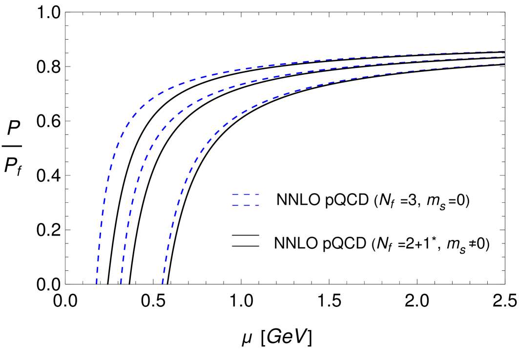
Figure 5: Left: the normalized pressure $\mathcal{P}_{\rm QCD,NNLO}^{N_{f}=2+1^{*}}/\mathcal{P}_{f}$ obtained from our reevaluated $G_{i}$ functions, Eq.(9), with residual scale dependence $\mu\leq\Lambda\leq 4\mu$. Right: relative difference with respect to KRV 2010 Kurkela:2009gj , with $\Delta P\equiv P(\mathrm{KRV\;2010})-P(\mathrm{this\;work})$.

The residual renormalization scale dependence is illustrated from taking $\mu\leq\Lambda\leq 4\mu$ as conventionally done in the literature. Note that the scale dependence of both $N_{f}=3$ and $N_{f}=2+1^{*}$ pQCD pressures in Fig. 7 appears slightly reduced as compared to Kurkela:2009gj , due to the exact NLO running coupling Eq.(15) producing slightly smaller scale variations for very low scale values, compared to the more standard running coupling given as an expansion in $\ln(\Lambda)^{-1}$PDG2018 . We also illustrate in Fig. 5 (right) the modifications induced from our updated $G_{i}$ fitting functions (notably $G_{2}$): comparing the two pressures obtained respectively from the previousKurkela:2009gj or with our new $G_{i}$ functions in Eq.(9), we observe that the $G_{2}(\hat{m})$ difference we obtained has a very moderate effect on the standard NNLO pressure values for $m_{s}\neq 0$: in the extreme case, for the scale $\Lambda=\mu$ and $\mu=0.7$ GeV, where $\alpha_{S}\approx 0.58$ is already very large, the difference is about $-4\%$ (noting that the updated $G_{2}$ gives a lower pressure for a given $\mu$ value). In contrast, the differences in $G_{2}$ will have more impact for our RGOPT construction, as the latter involves medium-dressed quark masses of order $\sim g\,\mu\gg m_{s}$, as it will be developed in next Section.

II.2.2 Pocket formula for pQCD $N_{f}=2+1^{*}$

Finally, for completeness, we provide a compact fitting function giving a good approximation of the full NNLO quark matter $N_{f}=2+1^{*}$ pressure, in the spirit of a similar approximation given in ref.prevN2LOfit :

$$\frac{\mathcal{P}_{\rm QCD}^{N_{f}=2+1^{*}}(\mu,\Lambda=X\,\mu)}{\mathcal{P}_{f}(\mu,N_{f}=3)}=\left(c_{1}+c_{2}X^{\nu_{3}}\right)-\frac{d_{1}(3\tilde{\mu})^{\alpha_{1}}X^{\nu_{1}}}{(3\tilde{\mu}-d_{2}\,X^{-\nu_{2}})},\ \ \ \tilde{\mu}=\mu/{\rm GeV},$$ (17)

$$c_{1}=0.830189,c_{2}=0.505545,d_{1}=0.438396,d_{2}=1.165107,\alpha_{1}=1.014939,$$

$$\nu_{1}=0.670277,\nu_{2}=0.899925,\nu_{3}=0.632526.$$

III RGOPT pressure at next-to-next-to-leading order for $N_{f}=3^{*}$

Although the quark sector of dense QCD does not exhibit proper IR divergences like for the soft gluon modes, it is nevertheless highly desirable to resum well-defined (RG-induced) higher orders as well in this sector, incorporating additional information beyond the strictly perturbative expansion. Accordingly, our main aim is to possibly further reduce in particular the residual renormalization scale dependence, that hampers to some extent the standard cold quark matter pressure perturbative expansion.

Quite similarly to the SPTspt1 ; spt3 or HTLptHTLpt framework, the RGOPT implies as a first step to modify the original QCD Lagrangian by adding and subtracting a Gaussian (quark) mass term, with one of the contribution being treated as an interaction. Although the specific mass dependence is at first the one dictated by the standard massive perturbative calculations, this mass is subsequently treated as a variational parameter, $\overline{m}$, not to be confused with the physical quark masses in the present context. More precisely, as will be derived in more details below, $\overline{m}$ is determinedRGOPTals ; rgopt_cold from a self-consistent mass gap upon imposing the pressure $P(\overline{m})$ to satisfy the RG equation at a given order of the modified expansion. This gives to $\overline{m}$ the properties of a medium-dressed quark mass, $\overline{m}(g,\mu\cdots)$, but embedding a RG-dictated all order coupling dependence. Accordingly, at successive orders of the modified expansion, the resulting pressure $P(\overline{m}(g,\mu,\cdots))$ gives a sequence of improved approximations to the initially massless quark limit of the theory.

To simplify, we first implement the RGOPT for degenerate (dressed) quark masses, i.e. the $N_{f}$ quark flavors are treated similarly, obtaining a common RG-dressed medium mass $\overline{m}(\mu)$, while the physical quark masses are neglected. Then we consider the more precise non-degenerate case, incorporating in this framework the extra contribution from the genuine strange quark (current) mass. Concretely, we have first to modify the previously considered $N_{f}=2+1^{*}$ pressure to implement $N_{f}=3^{*}$ degenerate massive quarks, followed by a generalization to unequal masses.

III.1 From $N_{f}=2+1^{*}$ to $N_{f}=3^{*}$ massive quarks

Upon examination of the relevant contributions, including the cancellations of UV divergences and renormalization terms, going from $N_{f}=2+1^{*}$ to $N_{f}=3^{*}$ massive quarks with an identical mass can be incorporated upon following the simple prescriptions:

$$\begin{array}[]{ccl}\mathcal{M}_{3}^{\rm 1c}&\to&\mathcal{M}_{3}^{\rm 1c}+(N_{f}-1)2(3-\pi^{2})\hat{m}^{2}z,\\ \mathcal{M}_{3}^{\rm 2c}&\to&\mathcal{M}_{3}^{\rm 2c}-(N_{f}-1)\frac{2}{3}I_{12},\\ \mathcal{M}_{3}^{\rm 3c}&\to&\mathcal{M}_{3}^{\rm 3c}\end{array}\Bigg{\}}\Rightarrow G_{4}(\hat{m})\to N_{f}G_{4}(\hat{m}),\ \ {\rm for}\ N_{f}=2+1^{*}\to 3^{*}$$ (18)

which accordingly modifies $\mathcal{M}_{3}^{N_{f}=2+1^{*}}$ to $\mathcal{M}_{3}^{N_{f}=3^{*}}$ in Eq.(8) with the same $G_{i}$ functions in Eq.(9), and then

$$P^{\rm N_{f}=3^{*}}_{\rm 2GI,VM}(m,\mu)=\frac{g^{4}}{(4\pi)^{3}}\mathcal{M}_{3}^{N_{f}=3^{*}}.$$ (19)

On top of Eq.(18), an extra overall factor of $N_{f}$ multiplies the contributions in Eq.(1), so that explicitly:

$$\mathcal{P}_{\rm NNLO}^{N_{f}=3^{*}}(m,\mu)=N_{f}\left(P_{\rm LO}(m,\mu)+P_{\rm NLO}(m,\mu)+P^{\rm N_{f}=3^{*}}_{\rm 2GI,VM}(m,\mu)\right)-\Omega^{N_{f}=3^{*}}_{\rm Ring}(m,\mu)\;.$$ (20)

Note that the vacuum-matter term $\Omega_{{\rm VM},x}^{N_{F}=3^{*}}$ appearing in Eq.(11) is now zero since $N_{l}=0$. Concerning next the ring contributions, care must be taken to avoid double counting contributions and other inconsistencies when generalizing the results from $N_{f}-1$ massless quarks plus a single massive quark, to $N_{f}$ massive quarks. The final expression reads

$$\Omega_{\rm Ring}^{N_{f}=3^{*}}=\frac{N_{f}^{2}d_{A}\ g^{4}\,\mu^{4}}{512\pi^{6}}\left[I_{13}\left(2\ln\left(\frac{g}{4\pi}\right)-\frac{1}{2}\right)+\frac{1}{2}\left(I_{20}+\frac{16}{3}(1-\ln 2)\ln(2)I_{21}+I_{23}\right)\right],$$ (21)

where the overall factor $N_{f}^{2}$ accounts for all degrees of freedom. Note that for this purpose ($N_{f}=3^{*}$) one has to define a new integral, $I_{23}$, generalizing $I_{22}$ of Eq.(II.1.3) to three massive quarks with the same mass and chemical potential. The definition of $I_{23}$ is

$$\begin{split}I_{23}(m,\mu)=&\frac{16}{\pi}\int_{0}^{\frac{\pi}{2}}d\phi\sin{\phi}^{2}\left(F_{h}^{2}(0,\phi,\hat{m})\ln(N_{f}F_{h}(0,\phi,\hat{m}))+\frac{1}{2}G_{h}^{2}(0,\phi,\hat{m})\ln(N_{f}G_{h}(0,\phi,\hat{m}))\right)\\ =&2\,I_{13}(m,\mu)\ln N_{f}+\delta(1-\hat{m}^{2})+\hat{m}^{2}\left(1.4000-2.2193\hat{u}\right)+\hat{m}^{4}\left(-2.4866+2.8318\hat{u}\right)+\hat{m}^{6}\left(1.0866-0.5860\hat{u}\right),\end{split}$$ (22)

where $\delta\approx-0.85638321$ was defined in pQCDmu4L , and $F_{h}$, $G_{h}$ are the same functions defined in Eq.(A11) of Kurkela:2009gj . The corrections from different chemical potential appear in $I_{20}$ and $I_{23}$ but have been neglected since their relative contribution is numerically completely negligible.

III.2 RGOPT modifications to the pressure

The next important modification with respect to the above weak-coupling expansion pressure in Eq.(1), is to supplement it with pure vacuum contributions: these are evidently vanishing for massless quarks, and even when considering the quark mass dependence these contributions are often justifiably neglected in the quark matter literature, on grounds that they depend solely on the mass $m$ and not on the in-medium $\mu$ scale. However, since RG properties are essentially related to UV divergences, and the latter are determined by the $T=\mu=0$ theory, these vacuum contributions play a crucial role in the massive RG invariance properties, as will be recalled below.

Up to NNLO, the complete contributions to the pure vacuum (including the VV part of the plasmon) pressure can be easily extracted from KNcond , modifying the above defined NNLO quark matter pressure expressions in Eqs.(2), (3), (8), as follows:

$$P_{\rm LO}(m,\mu)\to P_{\rm LO}(m,\mu)-N_{c}\frac{m^{4}}{8\pi^{2}}\left(\frac{3}{4}-L_{m}\right)\equiv P^{v+m}_{\rm LO}(m,\mu)$$ (23)

$$P_{\rm NLO}(m,\mu)\to P_{\rm NLO}(m,\mu) -\frac{d_{A}g^{2}}{4(2\pi)^{4}}m^{4}\left(3L_{m}^{2}-4L_{m}+\frac{9}{4}\right)\equiv P^{v+m}_{\rm NLO}(m,\mu)$$ (24)

$$P_{\rm NNLO}(m,\mu)\to P_{\rm NNLO}(m,\mu)+P^{v,d}_{\rm NNLO}(m,N_{f},N_{h},N_{l})\equiv P^{v+m}_{\rm NNLO}(m,\mu)$$ (25)

where $L_{m}=\ln(m/\Lambda)$, and

$$P^{v,d}_{\rm NNLO}(m,N_{f},N_{h},N_{l})\equiv \frac{g^{4}m^{4}}{\pi^{2}(4\pi)^{4}}\left(a_{3,3}+a_{3,2}\ L_{m}+a_{3,1}\ L_{m}^{2}+a_{3,0}\ L_{m}^{3}\right)$$ (26)

$$a_{3,3}= \ -\frac{23\,821}{144}-\frac{22}{3}\zeta(4)-\frac{8}{3}\zeta(2)(\log{2})^{2}+\frac{4}{9}(\log{2})^{4}+\frac{32}{3}\ {\rm Li}_{4}(1/2)-6\ \zeta(3)$$

$$+\frac{13}{12}N_{f}+N_{h}\left(\frac{367}{24}-\frac{28}{3}\ \zeta(3)\right)+N_{l}\left(\frac{45}{8}+\frac{8}{3}\zeta(3)\right)$$

$$a_{3,2}= \ \frac{3817}{12}-4\zeta(3)-\frac{13}{3}N_{f}-\frac{39}{2}N_{h}-\frac{15}{2}N_{l}$$

$$a_{3,1}= \frac{1}{3}\left(-807+26N_{f}\right)$$

$$a_{3,0}= \frac{4}{3}\left(81-2N_{f}\right)$$

where in the most general case $N_{l}$, $N_{h}$ are respectively the number of massless and massive quarks and $N_{f}\equiv N_{h}+N_{l}$. The “d” index at NNLO stands for diagonal since we will later distinguish the contributions from different quark masses in the “VV” diagram, Fig. 3, contained in Eq.(26). For the degenerate case $N_{f}=3^{*}$, we always have $N_{l}=0$ such that $N_{h}=N_{f}$, thus omitting here the argument. The generalization to $N_{f}=2^{*}+1^{*}$ in the next section is more subtle and will be addressed later.
This gives for the resulting complete NNLO vacuum and medium pressure contribution:

$$P^{v+m}(m,\mu)=P^{v+m}_{\rm LO}(m,\mu)+P^{v+m}_{\rm NLO}(m,\mu)+P^{v+m}_{\rm NNLO}(m,\mu)$$ (27)

In particular, it is easily seen from Eq.(23) and Eq.(2) that the $\ln(m)$ terms cancel via the recombination $\ln\frac{m}{\Lambda}+\ln\frac{\mu+p_{f}}{m}=\ln\frac{\mu+p_{f}}{\Lambda}$. Similarly, this cancellation also occurs at NLO. Now, note importantly that for arbitrary $m$ the pressure in Eq.(27) is not perturbatively RG invariant, as it explicitly depends on the renormalization scale $\ln(m/\Lambda)$ at LO, and within the original expression Eq.(27) this contribution cannot be canceled from $g(\Lambda)$ or $m(\Lambda)$ dependence, that would only affect higher orders. This is a known feature of any massive theories, actually related to their vacuum energy anomalous dimension. Accordingly, an important preliminary step of our construction is to obtain a (perturbatively) RG invariant (RGI) pressure, which implies to adding an extra zero point energy contribution, $S(m,g)$, to the pressureKNcond ; rgopt_phi4 :

$$P^{v+m}(m,\mu)\to P^{v+m}(m,\mu)-S(m,g)\equiv P^{v+m}(m,\mu)-\frac{m^{4}}{g^{2}}\sum_{k\geq 0}s_{k}\left(g^{2}\right)^{k}\equiv P^{v+m}_{\mathrm{RGI}}(m,\mu),$$ (28)

such that the latter combination is approximately scale-independent, at a given perturbative order. More precisely, the coefficients $s_{k}$ are determined at successive orders by applying the massive (homogeneous) RG operator

$$\Lambda\frac{d}{d\Lambda}=\Lambda\frac{\partial}{\partial\Lambda}+\beta(g^{2})\frac{\partial}{\partial g^{2}}-\gamma_{m}(g^{2})m\frac{\partial}{\partial m}\;,$$ (29)

on Eq.(28), requiring it to vanish up to neglected higher order terms. In our conventions the RG functions $\beta(g^{2})$ and $\gamma_{m}(g^{2})$ (the anomalous mass dimension) are given by

$$\beta\left(g^{2}\equiv 4\pi\alpha_{s}\right)=-2b_{0}g^{4}-2b_{1}g^{6}+\cdots\;,$$ (30)

and

$$\gamma_{m}\left(g^{2}\right)=\gamma_{0}g^{2}+\gamma_{1}g^{4}+\cdots\;,$$ (31)

with higher orders and explicit expressions collected in Appendix A. Accordingly, one obtains rgopt_cold

$$s_{0}=-N_{c}\left[(4\pi)^{2}(b_{0}-2\gamma_{0})\right]^{-1}\;,$$ (32)

and other relevant higher order $s_{k},k=1,\cdots,3$ coefficients are listed in Appendix A.
Note that in a fully equivalent way, $S(m,g)$ may be obtained from applying Eq.(29) as

$$\Lambda\frac{d}{d\Lambda}\left[S(m,g)\right]\equiv\hat{\Gamma}^{0}(g)m^{4}=m^{4}\sum_{k\geq 0}\Gamma^{0}_{k}g^{2k}$$ (33)

where $\hat{\Gamma}^{0}(g)$ defines the vacuum energy anomalous dimensionvacEn1 ; vacEn2 ; E0phi4 , similarly relevant for other massive theories, and adding an inhomogeneous contribution to the RG operator in Eq.(29). For QCD, $\hat{\Gamma}^{0}(g)$ has been determined up to five-loop ordervacEn5l . Notice that $S(m,g)$ only depends on the vacuum contributions and not on the medium ones. By construction the $s_{k}$ coefficients, even though being of order $k$-loops, encode RG information from order $k+1$.

Next, the RGOPT is implemented as the following stepsRGOPTals ; rgopt_cold :
1) First, reshuffling the interaction terms in the QCD Lagrangian, according to the replacements

$$m\to m\left(1-\delta\right)^{a},\;\;g^{2}\to\delta g^{2},$$ (34)

where in the present context $m$ is a quark mass. Eq.(34) can be most conveniently performed directly within the renormalized RGI massive pressure, Eq.(28): $\delta$ is a new expansion parameter, interpolating between the massive but free theory ($\delta\to 0$), and the massless interacting original theory, $\delta\to 1$, and the exponent $a$ will be specified below. For $a=1$ Eq.(34) is equivalent to the more familiar and intuitive “added and subtracted” mass term prescription, typically adopted in SPTspt1 ; spt3 or also in HTL perturbation theoryHTLptDense2L ; HTLptDense3L . Eq.(34) is consistent with standard mass renormalization, i.e. it does not add any new type of counterterms as long as one treats the mass counterterms within the modified $\delta$-expansion consistently with Eq.(34). As mentioned previously, we stress that $m$ is an arbitrary mass at this stage, determined from the prescription specified below.
2) Next, one expands the pressure resulting from Eq.(34) to the perturbative order in $\delta$ consistent with the usual perturbative expansion, then setting the result (after expansion) to $\delta\to 1$ suitable for the massless theory. Now importantly, RGOPT is based on observing that such a modified perturbative expansion may generally spoil the perturbative RGI properties of the original physical quantity (the pressure Eq.(28) in the case at hand): therefore the exponent $a$ in Eq.(34) is instead fixed (uniquely) such that RG invariance is recovered. Accordingly, applying the massless RG equation (i.e. with $m=0$ in Eq.(29)), to the LO RGOPT pressure, one obtains the critical valueRGOPTals ; rgopt_cold ; rgopt_hot

$$a=\frac{\gamma_{0}}{2b_{0}},$$ (35)

thus determined solely by the first order RG function coefficients.
3) Since step 2) leaves a remnant $m$-dependence at any finite $\delta$ orders, similarly to the OPTopt_pms (or HTLptHTLpt ; HTLptDense2L ) prescriptions, $m$ may be determined from requiring stationarity or mass optimization (OPT),

$$\frac{\partial P^{\rm{RGOPT}}}{\partial m}\Big{|}_{\overline{m}}=0\;,$$ (36)

giving a sequence of improved approximations at successive orders of the actually massless all order result. Accordingly $\overline{m}(g,\mu)$ is the nontrivial solution of a mass gap equation, akin to a medium-dressed mass.
4) According to our construction, $a$ is fixed once and for all at LO from Eq.(35), then used at higher orders of the $\delta$-expansion as a sensible way of comparing successive perturbative orders. Whereas at LO the RG equation is automatically fulfilled due to Eq.(35), at NLO and higher orders the resulting pressure no longer satisfies the RG Eq.(29), due to reshuffled mass dependence. Therefore, an alternativeRGOPTals to the OPT Eq.(36) is rather to (re)impose the RG Eq.(29), including RG coefficients consistently at the same perturbative order. The resulting nontrivial solution gives a “RG-dressed” medium mass, which by construction is expected to better restore the RG invariance of the pressure, as it includes higher order RG contributions. Actually, since we aim to recover the originally massless theory, it is more appropriate to determine $\overline{m}$ upon solving the reduced RG equation:

$$\left[\Lambda\frac{\partial}{\partial\Lambda}\mathcal{P}+\beta(g^{2})\frac{\partial}{\partial g^{2}}\mathcal{P}\right]_{\overline{m}_{RG}}=0\;.$$ (37)

Unfortunately, at NLO and higher orders, the exact solutions of either Eq.(36) or Eq.(37) are becoming highly nonlinear in $m$, with multiple $\overline{m}$ solutions appearing, some being non-real valued. Importantly, however, Eq.(35) also implies the compelling feature that at higher orders, the asymptotic freedom (AF) behavior for $\overline{m}(g\to 0)$ is obtained for only one of the solutionsRGOPTals .

IV RGOPT for cold quark matter

IV.1 NLO RGOPT

Before addressing the more involved results at NNLO, we briefly summarize the RGOPT results that were obtained at NLOrgopt_cold considering three flavors of quarks, corresponding to the graph in Fig. 1. With the genuine mass of the quarks being zero we end up with the chemical equilibrium condition $\mu_{s}=\mu_{u}=\mu_{d}\equiv\mu=\mu_{B}/3$. At this order there are still no gluons in the medium as they formally enter at the NNLO through the Ring diagrams. Starting from the known perturbative LO and NLO pressures in Eqs.(2)(3), supplemented by vacuum contributions Eqs(23),(24), these expressions are modified by Eq.(34), expanded to LO (NLO) $\delta^{0}$ ($\delta^{1}$), then finally taking $\delta\to 1$ to formally recover the massless limit. At LO, the RG equation being already used to fix Eq.(35), one uses Eq.(36) to determine $\overline{m}_{\rm LO}$, and RG invariance is exact at this one-loop order. For completeness, we give the LO mass gap obtained in rgopt_cold :

$$\overline{m}_{\rm LO}^{2}=\mu^{2}\left(\frac{\sqrt{1+4c\left(\overline{m}_{\rm LO},\mu,g^{2}\right)}-1}{2c\left(\overline{m}_{\rm LO},\mu,g^{2}\right)}\right),$$ (38)

with

$$c\left(\overline{m}_{\rm LO},\mu,g\right)=\left(\frac{1}{2b_{0}g^{2}}-\frac{1}{2}+L_{\mu}\right)^{2}\ \ \ ,\ \ \ L_{\mu}=\ln\left(\frac{\mu+p_{F}}{\Lambda}\right).$$ (39)

Applying next the same procedure (34) to the NLO pressure, Eqs.(23),(24), Eqs.(36) or (37) gave no real $\overline{m}$ exact solutionrgopt_cold on the full relevant $\mu$-value range. Invoking RG-invariance of the pressure under renormalization scheme change (RSC) up to perturbatively higher orders, one may slightly change the scheme to a one close to $\overline{\rm MS}$, such that a comparison remains perturbatively consistent, but modifying the RG equation coefficients to possibly recover real $\overline{m}$ solutionsRGOPTals . The NLO RSC is performed on the arbitrary mass $m$ according to

$$m\rightarrow m\left(1+B_{2}\ g^{4}\right),$$ (40)

to be applied prior to the variational modifications from Eq.(34), so that the RSC is defined in a standard perturbative manner. Notice that the higher order RG coefficients are also modified under the RSC (see Appendix A). Moreover, a definite prescription is needed to uniquely fix the RSC parameter $B_{2}$, arbitrary at this stage. FollowingRGOPTals ; rgopt_cold , the real solution closest to ${\overline{\mbox{\rm MS}}}$ is obtained when the two independent OPT and RG equations, Eqs.(36),(37), first intersect, respectively viewed as functions $f_{\rm OPT}(m,g^{2})\equiv 0$ and $f_{\rm RG}(m,g^{2})\equiv 0$ (i.e. when their respective tangent vectors are collinear). The latter prescription easily translates into a vanishing determinant condition:

$$\frac{\partial f_{\rm RG}}{\partial g^{2}}\frac{\partial f_{\rm OPT}}{\partial m}-\frac{f_{\rm RG}}{\partial m}\frac{\partial f_{\rm OPT}}{\partial g^{2}}\equiv 0.$$ (41)

Since the latter equation depends nontrivially on $B_{2}$, one solves it in conjunction with either Eq.(36) or Eq.(37) to obtain $(\overline{B}_{2},\overline{m})$ solutions. Following the previous prescription, the NLO RGOPT pressure was obtained in rgopt_cold , that we will not reproduce here. We simply remark that due to embedded RG invariance properties of $\overline{m}(g,\mu)$, the resulting pressure exhibits a more moderate sensitivity to residual renormalization scale variationsrgopt_cold , although the improvement is not as drastic as in the analogous construction at finite temperature and zero densityrgopt_hot .

IV.2 NNLO RGOPT

Next at NNLO, we include the RGOPT modifications of the relevant contributions in Fig. 2 as well as the plasmon contribution in Fig. 3, where the ring diagram, represented in Fig. 4, is given by Eq.(21). To recap, the perturbatively NNLO RG-invariant massive quark pressure $P_{RGI}^{v+m}$ as obtained in Eq.(28),(60) entails the contributions from Eqs.(27), with the NNLO contributions (25),(19). Then one applies on $P_{RGI}^{v+m}$ the modifications from Eqs.(34),(35) in the quark sector, these previously defined steps being formally summarized as:

$$P_{RGI}^{v+m}(m\to m(1-\delta)^{\frac{\gamma_{0}}{2b_{0}}},g\to\delta g)|_{\delta^{2},\delta\to 1}\equiv P_{\rm RGOPT}^{v+m}(m,g)\equiv P_{\rm RGOPT}^{N_{f}=3^{*}}(m,g).$$ (42)

The explicit expression resulting from Eq.(42) is not particularly illuminating so we do not display it here. Upon next using either the OPT Eq.(36) or the RG Eq.(37) to determine $\overline{m}$, we found no real solutions in the full relevant $\mu$ range. Thus, similarly to the NLO case, we perform a perturbative RSC in order to obtain real and continuous solutions in the full $\mu$ range, considering the same RSC Eq.(40) as was performed at NLO. After the modified expansion from Eq.(34), this induces contributions to the pressure that remain linear in $B_{2}$, therefore easier to handle analytically. Similarly to NLO, we can recover a real solution by requiring Eq.(41) to be satisfied. As a technical remark, while Eqs.(36),(37),(41) all have a very involved nonlinear $m$-dependence at NNLO, note that the RSC parameter $B_{2}$ may be first trivially obtained from the relevant RG Eq.(37), linear in $B_{2}$. Inserting the resulting solution $B_{2}(m,g,\cdots)$ into Eq.(41) provides a single equation for $m$, once fixing the other relevant parameters $g(\Lambda),\mu,\Lambda$. In this way the whole procedure to determine $\overline{m}(g,\mu,\Lambda)$ is analytically straightforward, although somewhat involved numerically.
While our prescription defines $\overline{m}_{RG}(g,\mu)$ from an RG-optimized pressure, thus unrelated to the standard Debye mass, defined from the pole of the quark propagator, we expect a consistent solution to behave at small $g^{2}$ as a screening mass in the medium, $\overline{m}^{2}\sim\#g^{2}\mu^{2}$, upon perturbative re-expansion. Accordingly, it is sensible to compare at least qualitatively our solutions with the $T=0$ perturbative Debye screening quark mass:

$$m^{2}_{\rm D}=\frac{g^{2}\,C_{F}}{8\pi^{2}}\mu^{2}.$$ (43)

It turns out that the $\overline{m}_{RG}(g,\mu)$ obtained from Eqs.(37) and (41) is remarkably close to $m_{D}$ (at least for moderate and high $\mu$ values in the perturbative range), as illustrated in Fig. 6. In contrast, using alternatively the OPT Eq.(36) with Eq.(41) gives a NNLO solution more than an order of magnitude smaller than $m_{D}$ for any $\mu$ values, which accordingly we do not consider a physically acceptable solution. Concerning the RSC parameter $\overline{B}_{2}(\mu)$ determined together with $\overline{m}_{RG}(\mu)$, for a given scale $\Lambda$ we obtain $B_{2}$ values almost constant for a large $\mu$ range, e.g. $\overline{B}_{2}\sim-0.025$ for $\Lambda=2\mu$. These relatively large values can be traced to the sizable (negative) departure from the massless quark NNLO pressure for a typical dressed mass $\simeq m_{\rm D}$, originating dominantly from $G_{1}(m/\mu),G_{2}(m/\mu)$ entering the NNLO massive contributions Eq.(8) (see Fig. 9), requiring a relatively sizable $|B_{2}|$ to recover real $\overline{m}_{RG}(\mu)$ solutions. However, importantly the fact that $\overline{m}_{RG}^{2}\sim\#g^{2}\,\mu^{2}$ for moderate $g$ guarantees that the modifications induced in the pressure from the RSC, $\propto\overline{B}_{2}\,g^{2}\overline{m}^{4},\overline{B}_{2}\,g^{4}\mu^{2}\overline{m}^{2}$ or higher orders, remain perturbatively formally of higher order ${\cal O}(g^{6})$.
In Fig. 6 we also illustrate the residual scale dependence of $\overline{m}_{RG}$ as compared to the perturbative Debye mass, Eq.(43). The scale dependence is moderately reduced, but once inserting $\overline{m}_{RG}$ in the RGOPT pressure,

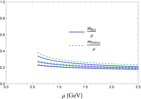
Figure 6: Residual scale dependence of the RG-determined mass $\overline{m}_{\rm RG}(g(\Lambda))$ for $\Lambda=2\mu X$ with $X=\frac{1}{2},1,2$ (from top to bottom curves respectively), compared with the LO Debye mass.

the latter exhibits a further reduced scale dependence, compared to the NNLO weak-coupling expansion pressure, as observed in Fig. 7. The NNLO pressure also shows a better scale dependence with respect to NLO RGOPTrgopt_cold . Overall, the reduction of scale dependence from RG resummation we obtain for cold dense matter is, however, not as efficient as its counterpart for hot QCDrgopt_hot . This may be explained by the already improved scale dependence and convergence of the standard weak-coupling expansion for cold quark matter, as compared to its counterpart for hot QCD.

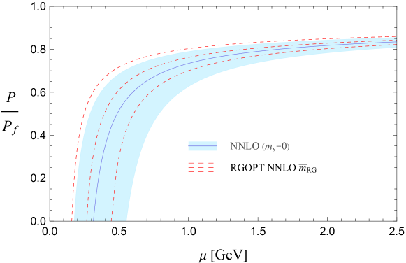
Figure 7: The RGOPT pressure $P_{\rm RGOPT}^{N_{f}=3^{*}}(\overline{m}_{RG})$, Eq.(42), compared to the NNLO pQCD pressure (massless and massive quarks as indicated) for three different scales $\Lambda=2\mu X$ with $X\in\left[\frac{1}{2},1,2\right]$ (from bottom to top curves)

Since the RG dressed mass is very close to the Debye mass $m_{\rm D}$ in Eq.(43), one may perhaps consider using the latter as a much simpler alternative mass prescription (as it is indeed done at finite temperature and densities for NNLO HTLptHTLptDense3L ). However, in this case the resulting pressure does not show any improved scale dependence with respect to the standard NNLO pressure. Likewise, perturbatively reexpandingrgopt_cold the $\overline{m}_{RG}$ solution would result in a degradation of the scale dependence, compared to the exact $\overline{m}_{RG}$. This illustrates that the RG-dressed mass is quite crucial to gain scale independence, due to the embedded higher RG order dependence.

On top of the previous RG improved NNLO results, one could wish to include a recently derived all order resummation of the HTL soft logarithmic dependence in the pure glue sectorFernandez:2021jfr . More precisely, the ring contribution discussed earlier is only the leading order of a sequence of non-analytic contributions in $g^{2}$ to the pressure. Going to higher orders, higher powers of $\ln g$ will appear due to IR divergences resummationsGorda:2021znl , and those contributions arise with a specific pattern, that happens to be dictated by the RG in an adequately defined effective field theory (EFT) set-upFernandez:2021jfr . This EFT is built on the hard thermal loops generated by the gluonsHTLbasic , hence the name HTL EFT. At the moment, only the leading logarithms ($g^{4}\ln g,\ g^{6}\ln^{2}g,\ g^{8}\ln^{3}g,\dots$) are completely resummed in this approach. However, it appears presently difficult to combine the gluon sector resummation results in Fernandez:2021jfr with the RGOPT approach performed here, as it would require to apply a similar variational procedure rather in the HTL EFT, with an effective gluon mass relevant for dense HTL. But missing higher order contributions prevents us from pursuing such considerations here, which are beyond our present scope and left for future work.

V Incorporating the Strange quark mass in RGOPT: $N_{f}=2^{*}+1^{*}$

V.1 Non-diagonal massive contributions at NNLO

So far, we discussed fully symmetric $N_{f}=3$ quark matter with RG-dressed masses $m_{1}=m_{2}=m_{3}\equiv\overline{m}_{RG}$ and chemical potentials $\mu_{1}=\mu_{2}=\mu_{3}\equiv\mu$. Reintroducing different chemical potentials is straightforward within the NNLO contribution $\mathcal{M}_{3}^{N_{f}=3^{*}}$, Eq.(19), but more involved in the ring contributions in Fig. 4. However, when accounting for beta-equilibrium and charge neutrality, since the electron chemical potential $\mu_{e}\ll\mu\equiv\mu_{d}=\mu_{s}$, it leads to very small differences among the three respective quark $\mu_{i}$ values. Moreover, the ring contribution being itself numerically subdominant for a large $\mu$ range with respect to other NNLO contributions, accounting for these differences would lead to completely negligible effects in the total pressure. Indeed, we anticipate that the strange quark mass effects, on top of the RG-dressed mass, are numerically quite irrelevant within the ring contributions, while the latter effects are typically an order of magnitude larger than unequal chemical potential contributions. After a lengthy numerical evaluation we found these modifications to be too small to be relevant at all. Therefore, as far as the ring contributions are concerned, for computational efficiency we stick to the $N_{f}=3^{*}$ massive ring results given earlier in Eq.(21).

In contrast, concerning the other largely dominant NNLO contributions to the pressure, Eqs.(19),(25), our goal now is to treat a more general case $(m_{1}=m_{2}=\overline{m}_{RG},\,m_{3}=\overline{m}_{RG}+m_{s})$, where $m_{s}$ is the genuine strange quark (running) mass. We anticipate that the latter is the relevant mass pattern within NNLO contributions, resulting from the appropriate generalization of Eq.(34) when incorporating $m_{s}\neq 0$, as will be clear below. Starting at $\mathcal{O}(\alpha_{s}^{2})$, there are new “mixed” (non-diagonal) contributions from having nondegenerate quark masses. This is easily observed from the plasmon displayed in Fig. 3) where two loops of independent quarks contribute. These effects from unequal masses are not a priori negligible, in particular for relatively low $\mu$ values where the NNLO contributions $\sim g^{4}(\Lambda\sim\mu)$ are enhanced, and at the same time the strange quark running mass $m_{s}(\Lambda\sim\mu)$ and RG-dressed mass $\overline{m}_{RG}(g,\mu)$ values may become roughly of similar order. The first contribution is purely a vacuum (VV) contribution, which has to be incorporated in Eq.(25). The second graph is incorporated in an appropriately modified $\mathcal{M}_{3}^{N_{f}=3^{*}}$ of Eq.(19), while the last one is part of the ring resummation. For a careful derivation of the modified vacuum contribution, see Appendix C. Collecting the result from Eq.(93), we find the replacement

$$N_{f}P^{v,N_{f}=3^{*}}_{\rm NNLO}\to P^{v,N_{f}=2^{*}+1^{*}}_{\rm NNLO} =\left(\frac{g^{4}}{\pi^{2}\,(4\pi)^{4}}\right)\bigg{(}(N_{f}-1)m^{4}\left(-156.833+253.775L_{m}-243L_{m}^{2}+100L_{m}^{3}\right)$$ (44)

$$\left.+2(N_{f}-1)m^{2}m_{3}^{2}\left(-4.75802-6\left(L_{m}+L_{m_{3}}\right)\right)\right.$$

$$+m_{3}^{4}\left(-152.075+265.775L_{m_{3}}-243L_{m_{3}}^{2}+100L_{m_{3}}^{3}\right)\bigg{)},$$

accounting for the $N_{f}^{2}$ degrees of freedom, with $L_{m}=\ln(m/\Lambda)$ and $L_{m_{3}}=\ln(m_{3}/\Lambda)$. Accordingly, the zero point energy terms in Eq.(28) must be modified similarly such as to preserve perturbative RG invariance, according to

$$-N_{f}\frac{m^{4}}{g^{2}}\sum_{k=0}^{2}s_{k}\,\left(g^{2}\right)^{k}\to P_{\rm sub}^{N_{f}=2^{*}+1^{*}}\equiv -(N_{f}-1)\frac{m^{4}}{g^{2}}\left(s_{0}+s_{1}\,g^{2}\right)-\frac{m_{3}^{4}}{g^{2}}\left(s_{0}+s_{1}\,g^{2}\right)$$ (45)

$$-(N_{f}-1)s_{2,1}m^{4}\,g^{2}-s_{2,3}\,m_{3}^{4}\,g^{2}-2(N_{f}-1)s_{2}^{nd}\,m^{2}m_{3}^{2}\,g^{2}.$$

(See appendix A for the explicit expressions of the $s_{i,j}$ coefficients).

The derivation of the “VM” graph with three different masses is more involved: details about the modifications implied for this new $\mathcal{M}_{3}^{N_{f}=2^{*}+1^{*}}$ are given in Appendix C.2. To keep track of the origin of the mass coming either from the vacuum or the matter loop, we rename the latter $m\to m_{i}$ according to $\mathcal{M}_{3}^{N_{f}=3^{*}}(m)\to\mathcal{M}_{3}^{N_{f}=2^{*}+1^{*}}(m_{i})$. In summary, to switch from the fully symmetric massive quarks ($N_{f}=3^{*}$) case to the more general $N_{f}=1^{*}+1^{*}+1^{*}$ case with different masses (from which $N_{f}=2^{*}+1^{*}$ is a specific case) amounts to apply the following modifications of the last terms in Eq.(8):

$$\begin{split}N_{f}\left(\frac{2}{3}\ln\frac{\hat{m}}{2}+\frac{11}{9}+G_{3}(\hat{m})+G_{4}(\hat{m})\right)\to&N_{f}\left(\frac{2}{3}\ln\frac{\hat{m}_{i}}{2}+\frac{11}{9}+G_{3}^{\rm bis}(\hat{m}_{i})\right)+\hat{m}_{i}^{2}z(m_{i})\sum_{j}^{N_{f}}\Bigg{\{}{\rm Li}_{2}(\nu_{ij})\left(1+\nu_{ij}^{-2}\right)\\ &-\Phi\left(\nu_{ij},2,\frac{3}{2}\right)\left(1+\nu_{ij}\right)-\nu_{ij}^{-2}+\mathcal{F}(\nu_{ij})\Bigg{\}}-\sum_{j}^{N_{f}}\frac{4}{3}I_{12}^{\rm bis}(\hat{m}_{i},\nu_{ij}),\end{split}$$ (46)

where $\nu_{ij}=(m_{i}/m_{j})^{2}$, $\mathcal{F}(\nu_{ij})$ is defined in Eq.(97), $\Phi(a,b,c)$ is the Lerch Zeta function, ${\rm Li}_{2}$ is the Polylogarithm function and we conveniently provide $G_{3}^{\rm bis}$ as a rather accurate fitting function, quite similarly to those in Eq.(9):

$$G_{3}^{\rm bis}(\hat{m})=32\pi^{4}\hat{m}^{2}\Big{(}-0.000244-0.003777\hat{u}+0.000319\hat{u}^{2}+0.001263\hat{u}^{3}+0.000322\ln\hat{m}+0.000572\ln^{2}\hat{m}+0.003743\hat{m}^{2}\ln\left(\frac{1+\hat{u}}{\hat{m}}\right)\Big{)}.$$ (47)

In addition, the definition and a more convenient two-dimensional fit of the integral $I_{12}^{\rm bis}$ is given in appendix C.3. To recover the massless limit, one must first take the limit $\nu_{ij}\to 1\,\forall\>i,\,j$, where all masses become identical, and only then taking the limit $m\to 0$. (Upon taking the former limits, we correctly reproduce the left-hand side of Eq.(46) as a crosscheck).
Finally to recap, the complete $N_{f}=2^{*}+1^{*}$ QCD pressure reads

$$\mathcal{P}_{\rm QCD,NNLO}^{N_{f}=2^{*}+1^{*}}(m,m_{s},\mu)= (N_{f}-1)\left(P_{\rm LO}(m,\mu)+P_{\rm NLO}(m,\mu)+P_{\rm 2GI,VM}^{N_{f}=2^{*}+1^{*}}(m,\mu)\right)+P_{\rm LO}(m_{3},\mu)+P_{\rm NLO}(m_{3},\mu)$$ (48)

$$+P_{\rm 2GI,VM}^{N_{f}=2^{*}+1^{*}}(m_{3},\mu)-\Omega_{\rm Ring}^{N_{f}=2^{*}+1^{*}}+P_{\rm NNLO}^{v,N_{f}=2^{*}+1^{*}}+P_{\rm sub}^{N_{f}=2^{*}+1^{*}},$$

where, as above explained, we made the legitimate approximation $\Omega_{\rm Ring}^{N_{f}=2^{*}+1^{*}}\approx\Omega_{\rm Ring}^{N_{f}=3^{*}}$.

From here, we apply the RGOPT procedure as detailed in section III, Eqs.(34)-(37), with the modification that Eq.(34) is now generalized to

$$m_{i}\to m\left(1-\delta\right)^{{\frac{\gamma_{0}}{2b_{0}}\,}},\ i=1,2\$$ (49)

$$m_{3}\to m\left(1-\delta\right)^{{\frac{\gamma_{0}}{2b_{0}}\,}}+m_{s}$$

$$\;g^{2}\to\delta g^{2},$$

accordingly importantly the genuine physical mass $m_{s}$ remains unaffected by the $\delta$-expansion. This leads to a corresponding generalization of Eq.(42) for $m_{s}\neq 0$. Upon recovering $\delta\to 1$ after the appropriate $\delta$-expansion being performed up to NNLO ($\delta^{2}$), notice that the originally NNLO $m$-dependent contributions, being already ${\cal O}(g^{4})$, are simply obtained from $m\to m+m_{s}\equiv m_{3}$ concerning the strange quark contributions, due to the last term in Eq.(49). Accordingly, this brings NNLO contributions of the form derived above in Eqs.(44), (45), (46) as anticipated. An additional important modification as compared to $m_{s}=0$ is that the RG operator has to be consistently extended by introducing the strange quark anomalous mass dimension within Eq.(37),

$$\Lambda\frac{d}{d\Lambda}=\Lambda\frac{\partial}{\partial\Lambda}+\beta(g^{2})\frac{\partial}{\partial g^{2}}-m_{s}\gamma_{m_{s}}\frac{\partial}{\partial m_{s}}.$$ (50)

Note indeed that if restricting Eq.(48) to LO, Eq.(49) breaks explicitly, by ${\cal O}(m_{s}/m)$ terms, the exact RG-invariance of the LO pressure previously satisfied for arbitrary $m$, resulting from the critical exponent in Eq.(35). However, similarly to our NLO and NNLO prescription for $m_{s}=0$, the massive LO RG invariance can be simply recovered upon reimposing Eq.(50): it gives an already nontrivial LO screening mass solution, behaving for sufficiently small $m_{s}$ as $\overline{m}_{RG,LO}\sim\#g\mu+{\cal O}(m_{s})$. Next proceeding at NNLO, applying the complete RGOPT prescription with $m_{s}\neq 0$ is slightly more involved but conceptually very similar to the procedure described above in Sec.IV.2, so that we basically use now the massive RG Eq.(50), after having performed the RSC according to Eqs.(40),(41), the latter being required in order to recover real $\overline{m}_{RG}$ solutions. Due to nonlinear $m$, $m_{s}$ dependencies, the solutions $\overline{m}_{RG}(m_{s})$ are not related in a simple manner to $\overline{m}_{RG}(0)$ obtained in Fig. 6, but one always get $\overline{m}_{RG}(m_{s})<\overline{m}_{RG}(0)$, which can be understood since $m_{s}\neq 0$ gives additional positive contributions to the pressure. As expected, this effect is relatively small for very perturbative $\mu,\Lambda$ values, while it becomes more important for very low $\mu$ and $\Lambda=\mu$, i.e. large $\alpha_{s}(\Lambda)$ values.

V.2 NNLO RGOPT pressure for $N_{f}=2^{*}+1^{*}$

Inserting the obtained $\overline{m}_{u,d}\equiv\overline{m}_{\rm RG},\ \overline{m}_{3}\equiv\overline{m}_{\rm RG}(m_{s})+m_{s}$ masses into Eq.(48) gives our final result for the $N_{f}=2^{*}+1^{*}$ pressure, accounting also for the running $m_{s}(\Lambda)$ from Eq.(16). The resulting pressure with its remnant scale dependence is displayed in Fig. 8, compared with the standard NNLO pQCD pressure ($N_{f}=2+1^{*}$), Eq.(14), and with the RGOPT pressure for symmetric quark matter ($N_{f}=3^{*}$), $P_{RGOPT}^{v+m}(\overline{m}_{RG})$ in Eq.(42). Importantly, we observe that our result lies within the uncertainty range of the standard NNLO QCD pressure but with a significantly reduced scale dependence with respect to the latter. Remark that the relative difference between respectively the resummed RGOPT pressures for massless quark and for $m_{s}\neq 0$ appears rather important for low $\mu$ values, as could be expected since $m_{s}(\Lambda)/\mu$ is not that small. For instance, for the central scale $\Lambda=2\mu$ and $\mu=0.5$ GeV, where $\alpha_{s}\simeq 0.4$, the RGOPT pressure for $m_{s}\neq 0$ is reduced by $\sim 20\%$ with respect to the massless pressure. This effect, however, is roughly comparable to the corresponding $m_{s}\neq 0$ effect for the standard NNLO pressure, comparing the latter in Fig. 5 (left).
We remark also that the threshold of the Heaviside $\theta(\mu-(\overline{m}+m_{s}))$ function is never reached, down to the lowest $\mu$ values here considered, therefore, the strange quark always populates the quark matter medium. The RGOPT pressure for the central scale ($\Lambda=2\mu$) reaches zero value for a somewhat smaller critical $\mu_{c}(\approx 0.338$ GeV) than the pQCD one ($\mu_{c}\approx 0.364$ GeV). This, in addition with the reduced scale dependence, is expected to have interesting consequences for the EoS relevant to compact stars. Such considerations, however, are beyond the scope of this work.

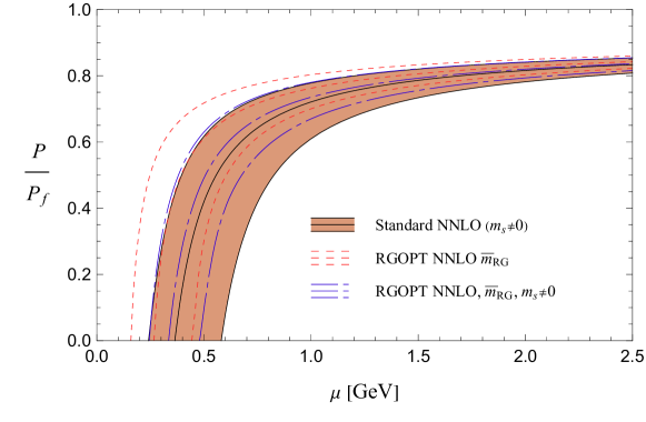
Figure 8: The RGOPT $N_{f}=2^{*}+1^{*}$ pressure compared to the NNLO pQCD $N_{f}=2+1^{*}$ pressure for $\Lambda=2\mu X$ with $X\in\left[\frac{1}{2},1,2\right]$ (from bottom to top curves).

V.2.1 Pocket formula for the RGOPT $N_{f}=2^{*}+1^{*}$ pressure

Finally, the procedure to reproduce our final results for $N_{f}=2^{*}+1^{*}$ being rather involved, we provide a simpler pocket formula as a good fit to the numerical RGOPT pressure result in Fig. 8, inspired from a similar construction in prevN2LOfit :

$$\frac{\mathcal{P}_{\rm RGOPT}^{N_{f}=2^{*}+1^{*}}(\mu,\Lambda=X\,\mu)}{\mathcal{P}_{f}(\mu,N_{f}=3)}=\left(c_{1}+c_{2}X^{\nu_{3}}\right)-\frac{d_{1}(3\tilde{\mu})^{\alpha_{1}}X^{\nu_{1}}}{(3\tilde{\mu}-d_{2}\,X^{-\nu_{2}})},\ \ \ \tilde{\mu}=\mu/{\rm GeV},$$

$$c_{1}=0.766035,c_{2}=0.501495,\alpha_{1}=0.996305,d_{1}=0.402405,d_{2}=0.974897,$$

$$\nu_{1}=0.410395,\ \nu_{2}=0.631054,\ \nu_{3}=0.366230.$$ (51)

VI Summary and conclusion

In this work we have applied the RGOPT resummation approach at NNLO to the cold quark matter pressure. As a preliminary basic ingredient of this approach, we have re-investigated the derivation of the NNLO massive cold quark matter pressure for two massless and one massive quark ($N_{f}=2+1^{*}$), originally evaluated in Kurkela:2009gj . While we have reproduced all analytical intermediate and final results from the latter work, we obtain a mismatch in one of the numerical fitting function ($G_{2}$) for massive integrals which, however, has a small impact on the standard NNLO pQCD pressure result, due to the moderate $m_{s}(\Lambda)$ relevant values. Then, we have proceeded to derive the RGOPT resummation at NNLO, first for the simpler degenerate $N_{f}=3^{*}$ case, and next for the more realistic $N_{f}=2^{*}+1^{*}$ case, the latter incorporating effects from the genuine strange quark mass. This involves first some modifications required to incorporate a fully symmetric massive pressure ($N_{f}=3^{*}$), followed by the more general case of non-symmetric massive pressure ($N_{f}=1^{*}+1^{*}+1^{*}$). In either case, our procedure embeds a higher order RG-dependence, and our results display a significantly reduced scale dependence with respect to the standard NNLO pressure Kurkela:2009gj . The latter RG resummation improvements appear, however, not as efficient as their counterpart for hot QCDrgopt_hot or for a hot scalar theoryrgopt_phi4_NNLO at NNLO. This is likely explained by the already better scale dependence and convergence properties of the weak-coupling expansion for cold quark matter, as compared typically to hot QCD. The RGOPT improvements should follow up for the EoS of cold quark matter in the same approximation, thereby potentially reducing the present pQCD uncertainties in the intermediate $\mu_{B}$ regime very relevant for the properties of compact stars.

VII Acknowledgements

We are very thankful to Aleksi Vuorinen for discussions, and for providing us useful intermediate numerical results related to Kurkela:2009gj for more precise comparisons. L.F. has been supported in part by the Research Council of Finland grants no. 353772 and 354533. L.F. is also grateful to the University of Montpellier where this work was started.

Appendix A

A.1 Renormalization group functions and counterterms

We give here relevant expressions for the coefficients of the RG functions $\beta(g^{2})$, $\gamma_{m}(g^{2})$ as well as the subtraction coefficients entering $S(m,g)$ in Eq.(28). Up to three-loop order (NNLO) one has

$$\beta\left(g^{2}\equiv 4\pi\alpha_{s}\right)=-2g^{4}\left(b_{0}+b_{1}g^{2}+b_{2}g^{4}+\mathcal{O}\left(g^{6}\right)\right)\;,$$ (52)

$$\gamma_{m}\left(g^{2}\right)=g^{2}\left(\gamma_{0}+\gamma_{1}g^{2}+\gamma_{2}g^{4}+\mathcal{O}\left(g^{6}\right)\right)\;,$$ (53)

with the successive order coefficients, for the relevant QCD case with $C_{A}=N_{c}$, $C_{F}=4/3$, $N_{c}=3$, but keeping the number of quark flavors $N_{f}$ unspecified:

$$b_{0}= h\left({\frac{11}{3}\,}C_{A}-\frac{2}{3}N_{f}\right)\ \ ,\ \ b_{1}=h^{2}\left({\frac{34}{3}\,}C_{A}^{2}-2C_{F}N_{f}-{\frac{10}{3}\,}C_{A}N_{f}\right)\ \ ,\ \ b_{2}=h^{3}\left(\frac{2857}{2}-\frac{5033}{18}N_{f}+\frac{325}{54}N_{f}^{2}\right)$$ (54)

$$b_{3}= h^{4}\left(\frac{149753}{6}+3564\zeta(3)-\Big{(}\frac{1078361}{162}+\frac{6508}{27}\zeta(3)\Big{)}N_{f}+\Big{(}\frac{50065}{162}+\frac{6472}{81}\zeta(3)\Big{)}N_{f}^{2}+\frac{1093}{729}N_{f}^{3}\right)$$

with $h=1/(4\pi)^{2}$,

$$\gamma_{0}= 2h(N_{c}C_{F}),\ \ \ \gamma_{1}=2h^{2}\left({\frac{3}{2}\,}C_{F}^{2}+{\frac{97}{6}\,}C_{F}C_{A}-{\frac{5}{3}\,}C_{F}N_{f}\right),\ \ \gamma_{2}=2h^{3}\left(1249+N_{f}\left(\frac{-2216}{27}-\frac{160}{3}\zeta(3)\right)-\frac{140}{81}N_{f}^{2}\right)$$ (55)

$$\gamma_{3}= 2h^{4}\Big{(}\frac{4603055}{162}+\frac{135680}{27}\zeta(3)-8800\zeta(5)+\Big{(}-\frac{91723}{27}-\frac{34192}{9}\zeta(3)+880\zeta(4)+\frac{18400}{9}\zeta(5)\Big{)}N_{f}$$

$$+\Big{(}\frac{5242}{243}+\frac{800}{9}\zeta(3)-\frac{160}{3}\zeta(4)\Big{)}N_{f}^{2}+\Big{(}-\frac{332}{243}+\frac{64}{27}\zeta(3)\Big{)}N_{f}^{3}\Big{)}.$$

Next, the coupling and mass counterterms are defined in our normalization conventions and with $D=4-2\varepsilon$, as

$$g_{0}^{2} \equiv g^{2}Z_{g}=g^{2}\left(1-g^{2}{\frac{b_{0}}{\varepsilon}\,}+g^{4}({\frac{b_{0}^{2}}{\varepsilon^{2}}\,}-{\frac{b_{1}}{2\varepsilon}\,})+{\cal O}(g^{6})\right)$$

$$m_{0} \equiv mZ_{g}=m\left(1-g^{2}{\frac{\gamma_{0}}{2\varepsilon}\,}+g^{4}({\frac{\gamma_{0}(2b_{0}+\gamma_{0})}{8\varepsilon^{2}}\,}-{\frac{\gamma_{1}}{4\varepsilon}\,})+{\cal O}(g^{6})\right),$$ (56)

where $g_{0}$, $m_{0}$ are the bare coupling and mass. Without going into full details, we simply remark that essentially taking the LO and NLO contributions in Eqs.(2),(3) formally with $m\to m_{0}$, $g\to g_{0}$ and using Eq.(A.1) cancels the explicit UV divergences initially present in the 1-cut and 2-cut contributions (see Eqs.(91), (97), (98)), resulting into the finite contributions Eqs.(5),(6).
The vacuum energy counterterm $Z_{0}$ is defined asvacEn2 ; vacEn5l

$${\cal E}_{0}^{B}\equiv\Lambda^{-2\varepsilon}\left({\cal E}_{0}(g^{2})-m^{4}\,Z_{0}(g^{2})\right)$$ (57)

where ${\cal E}_{0}^{B},{\cal E}_{0}$ are respectively the bare and renormalized vacuum energies and $Z_{0}$ the dimensionless counterterm (that cancels divergences originally present only in the vacuum contributions, that are not cancelled after coupling and mass renormalization). From this follows the vacuum energy anomalous dimension, that reads in our normalization:

$$\hat{\Gamma}^{0}(g^{2})=(-4\gamma_{m}(g^{2})-2\varepsilon)Z_{0}(g^{2})+\overline{\beta}(g^{2})\frac{\partial}{\partial g^{2}}Z_{0}(g^{2})\equiv\sum_{k\geq 0}\Gamma^{0}_{k}g^{2k}$$ (58)

with $\overline{\beta}(g^{2})\equiv-2\varepsilon g^{2}+\beta(g^{2})$ as it is appropriate for bare quantities. Explicitly, the vacuum energy anomalous dimension coefficients are (translated into our normalization from vacEn2 ; vacEn5l )

$$\Gamma^{0}_{0}=-2hN_{c},\ \ \Gamma^{0}_{1}=-2h\frac{N_{c}}{(4\pi^{2})}C_{F},\ \ \Gamma^{0}_{2}=-2h\frac{N_{c}}{(4\pi^{2})^{2}}\left(\frac{457}{72}-\frac{29}{12}N_{h}-\frac{2}{3}\zeta(3)-\frac{5}{12}N_{l}\right),$$ (59)

$$\Gamma^{0}_{3}=-2h\frac{N_{c}}{(4\pi^{2})^{3}}\left(33.6625-32.5586N_{h}+0.18139N_{h}^{2}+0.214632N_{h}\,N_{l}-4.96507N_{l}+0.0332417N_{l}^{2}\right),$$

where generically $N_{h},N_{l}$ are respectively the number of massive and massless flavor of quarks.

Note that the NLO in Eq.(A.1) is sufficient for the mass renormalization counterterm within the medium contributions, while higher order RG coefficients enter the RG-restoring coefficient $s_{k}$ in Eq.(28), those being only relevant for the pure vacuum contributions. These $s_{k}$ are determined from Eq.(28) or equivalently alternatively from Eq.(33) with Eq.(59), which gives explicitlyKNcond

$$s_{0}= \frac{\Gamma^{0}_{0}}{2\big{(}b_{0}-2\gamma_{0}\big{)}}=\frac{3}{7}\ \ ,\ \ s_{1}=\frac{1}{2\gamma_{0}}\left((b_{1}-2\gamma_{1})s_{0}-\frac{\Gamma^{0}_{1}}{2}\right)=-\frac{53}{224\pi^{2}}$$ (60)

$$s_{2}(N_{h},N_{l})= \frac{1}{b_{0}+2\gamma_{0}}\left((b_{2}-2\gamma_{2})s_{0}-2\gamma_{1}s_{1}-\frac{\Gamma^{0}_{2}}{2}\right)\underset{N_{h}=3,N_{l}=0}{=}-0.00040082$$

$$s_{3}(N_{h},N_{l})= \frac{1}{2(b_{0}+\gamma_{0})}\left((b_{3}-2\gamma_{3})s_{0}-2\gamma_{2}s_{1}-(b_{1}+2\gamma_{1})s_{2}-\frac{\Gamma^{0}_{3}}{2}\right)\underset{N_{h}=3,N_{l}=0}{=}-0.00008304.$$

Next, for the unequal quark mass case, dubbed as $N_{f}=2^{*}+1^{*}$ in the main text, the appropriate RG-restoring subtraction terms, as defined in Eq.(45), are determined as

$$s_{2,1}=s_{2}(N_{h}=2,N_{l}=1)=-0.00024683,\ \ \ s_{2,3}=s_{2}(N_{h}=1,N_{l}=2)=-0.00009284,\ \ s_{2}^{nd}=\frac{9}{8\pi^{4}(2N_{f}-81)}$$ (61)

A.2 Renormalization scheme change

For the relevant RSC, Eq.(40), one should account that it also affects RG coefficientsCollins . Accordingly, this induces the following modificationsRGOPTals :

$$\gamma_{2} \to\gamma_{2}^{\prime}=\gamma_{2}-4b_{0}\,B_{2}$$ (62)

$$\gamma_{3} \to\gamma_{3}^{\prime}=\gamma_{3}-4b_{1}\,B_{2}$$

$$s_{2}\to s_{2}^{\prime}=s_{2}+\frac{8b_{0}s_{0}}{b_{0}+2\gamma_{0}}B_{2}=-0.00040082+\frac{216}{175}B_{2},$$ (63)

$$s_{2,i}\to s_{2,i}^{\prime}=s_{2,i}+\frac{216}{175}B_{2},\,i=\{1,3\}$$

$$(s_{2}^{nd})^{\prime}=s_{2}^{nd}$$

$$s_{3}\to s_{3}^{\prime}=s_{3}+\frac{4B_{2}}{b_{0}+\gamma_{0}}\left(b_{0}s_{1}-\frac{b_{0}}{4}(a_{10}+4a_{11})+2\frac{s_{0}}{b_{0}+2\gamma_{0}}(b_{1}\gamma_{0}-b_{0}\gamma_{1})\right)=-0.00008304-\frac{111}{280\pi^{2}}B_{2}$$ (64)

where $a_{10}=-2(b_{0}-2\gamma_{0})s_{0}$, $a_{11}=-(3/4)a_{10}$.

Appendix B Massive integrals and fitting functions

Most basic integrals for the quark mass dependence were originally defined and evaluated in Kurkela:2009gj or given as supplemental material in WebSiteRomatchke . We give here some details on our reevaluation of the fitting functions $G_{i}(x)$ entering Eq.(8), obtained as combinations of the basic massive integrals $I_{k},k=1\cdots 12$ entering 2-cut and 3-cut contributions, Eqs.(6),(7). As mentioned in Sec. II, the $m\to 0$ limit of Eq.(8) is very nontrivial due to apparent $\ln(m)$ divergences, and the fitting procedure can be guided by the necessary cancellations of such IR divergent terms together with the knownpQCDmu4L $m\to 0$ limit of Eq.(8), and from inferring the $m\to 0$ limit of some of the $I_{k}$. There are first analytically integrable ones:

$$I_{1}(\hat{m})=\int\frac{d^{3}p}{(2\pi)^{3}}\frac{\Theta(\mu-E_{p})}{2E_{p}}\equiv\int_{p}=\frac{\mu^{2}}{8\pi^{2}}\,z,$$ (65)

$$I_{2}(\hat{m})=\int_{p}\int_{q}\frac{1}{(P-Q)^{2}}=\frac{\mu^{2}}{64\pi^{2}}\,\frac{\hat{u}^{4}-z^{2}}{\hat{m}^{2}}\underset{m\to 0}{=}\ -\frac{\mu^{2}}{64\pi^{2}}\,\left(1+2\ln\left(\frac{\hat{m}}{2}\right)+{\cal O}(\hat{m}^{2})\right)$$ (66)

$$I_{1b}(\hat{m})={\frac{\partial}{\partial\widetilde{m}^{2}}\,}\int_{p}={\frac{1}{8\pi^{2}}\,}{\frac{z-\hat{u}}{\hat{m}^{2}}\,}\underset{m\to 0}{=}\ \frac{1}{8\pi^{2}}\,\ln\left(\frac{\hat{m}}{2}\right)+{\cal O}(\hat{m}^{2})$$ (67)

$$I_{2b}(\hat{m}) = {\frac{\partial}{\partial\widetilde{m}^{2}}\,}\int_{p}\int_{q}{\frac{1}{(P-Q)^{2}}\,}={\frac{1}{128\pi^{4}}\,}\Bigg{\{}\left({\rm arctan}\left({\frac{\hat{u}}{\hat{m}}\,}\right)\right)^{2}-{\frac{2\hat{u}}{\hat{m}}\,}{\rm arctan}\left({\frac{\hat{u}}{\hat{m}}\,}\right)-\left(\ln\left({\frac{1+\hat{u}}{\hat{m}}\,}\right)\right)^{2}\Bigg{\}}$$ (68)

$$\underset{m\to 0}{=}\ \frac{1}{128\pi^{4}}\left(-\frac{\pi}{\hat{m}}+2+\frac{\pi^{2}}{4}-\ln^{2}\left(\frac{\hat{m}}{2}\right)+{\cal O}(\hat{m})\right)$$

$$I_{8}(\hat{m}) = \int_{p}\int_{q}\left(1-{\frac{E_{q}}{E_{p}}\,}\right){\frac{1}{\left((P-Q)^{2}\right)^{2}}\,}=-\frac{1}{128\pi^{4}}\left(\frac{\hat{u}}{\hat{m}}-{\rm arctan}\left(\frac{\hat{u}}{\hat{m}}\right)\right)^{2}$$ (69)

$$\underset{m\to 0}{=}\ \frac{1}{128\pi^{4}}\left(-\frac{1}{\hat{m}^{2}}+\frac{\pi}{\hat{m}}-1-\frac{\pi^{2}}{4}+{\cal O}(\hat{m})\right)$$

where $\hat{m},\hat{u},z$ were defined after Eq.(5), and we give straightforward $m\to 0$ limits. Note that in all integrals $P,Q,...$ are Euclidean on-shell four-momenta, i.e. $P^{2}=Q^{2}=-m^{2}$, and the remaining integrals $\int_{p},\int_{q}$ are three-dimensional with $p_{F}$ as cutoff, as explicit in Eq.(65). Moreover, $\partial_{\widetilde{m}^{2}}$ outside the integral acts only on the mass in the $p$-integration measure, after which $\widetilde{m}^{2}=m^{2}$ is set. Remark also the useful relation:

$$2(I_{2b}+I_{8})-{\frac{\partial\,I_{2}}{\partial m^{2}}\,}=0$$ (70)

where now $\partial_{m^{2}}$ is the standard full derivative. Next, the other relevant integrals can only be performed numerically, these are reproduced below from Kurkela:2009gj for convenience for the following discussion:

$$I_{1c}(\hat{m}) = \int_{p}\int_{q}\ln\left(\frac{(P-Q)^{2}}{m^{2}}\right)$$ (71)

$$I_{2c}(\hat{m}) = \int_{p}\int_{q}\frac{1}{(P-Q)^{2}}\ln\left(-\frac{(P-Q)^{2}}{m^{2}}\right)$$ (72)

$$I_{3}(\hat{m}) = \int_{p}\int_{q}\int_{r}{\frac{1}{(P-Q)^{2}(P-R)^{2}}\,},$$ (73)

$$I_{3b}(\hat{m}) = {\frac{\partial}{\partial\widetilde{m}^{2}}\,}\int_{p}\int_{q}\int_{r}{\frac{1}{(P-Q)^{2}(P-R)^{2}}\,},$$ (74)

$$I_{4}(\hat{m}) = \int_{p}\int_{q}\int_{r}{\frac{(Q-R)^{2}}{(P-Q)^{2}(P-R)^{2}}\,},$$ (75)

$$I_{5}(\hat{m}) = \int_{p}\int_{q}\int_{r}{\frac{1}{(P-Q-R)^{2}+m^{2}}\,},$$ (76)

$$I_{6}(\hat{m}) = \int_{p}\int_{q}\int_{r}{\frac{1}{(P-Q)^{2}(P-R)^{2}\left((P-Q-R)^{2}+m^{2}\right)}\,},$$ (77)

$$I_{7}(\hat{m}) = \int_{p}\int_{q}\int_{r}{\frac{(P-Q)^{2}}{(P-R)^{2}\left((P-Q-R)^{2}+m^{2}\right)}\,},$$ (78)

$$I_{9}(\hat{m}) = \int_{p}\int_{q}\int_{r}\left(1-{\frac{E_{q}}{E_{p}}\,}\right){\frac{2}{\left((P-Q)^{2}\right)^{2}\,(P-R)^{2}}\,},$$ (79)

where all integrals $I_{3}-I_{7}$ and $I_{9}$ require six-dimensional integration over three momenta $p,q,r$ and three angles. The last three integrals entering the 2-cut contributions are, defining $a=(P-Q)^{2}/m^{2}=-2+2(E_{p}E_{q}-p.q)/m^{2}$,

$$I_{10}(\hat{m}) = \int_{p}\int_{q}\Bigg{\{}-\frac{23}{3}+\frac{8}{a}-\ln(a)+\sqrt{\frac{a}{4+a}}\Bigg{[}-\pi^{2}\left(1+\frac{4}{3a^{2}}\right)+\ln^{2}(a)-2h_{1}^{2}(a)+\frac{8\ln(a)}{a^{2}}h_{3}(a)$$ (80)

$$+\left(\frac{4}{a^{2}}-1\right)\Big{(}\ln^{2}(4+a)-2h_{2}^{2}(a)+4h_{5}(a)\Big{)}+4h_{4}(a)\Bigg{]}+\sqrt{\frac{4+a}{a}}\left(\frac{4}{a}-3\right)h_{3}(a)\Bigg{\}},$$

$$I_{11}(\hat{m}) = -16m^{2}I_{1}I_{1b}+32m^{4}I_{2b}+\int_{p}\int_{q}\Bigg{\{}12+\frac{32}{a^{2}}(1-\frac{E_{q}}{E_{p}})+\left(2-\frac{8}{a}\right)\ln(a)+\sqrt{\frac{a}{4+a}}\Bigg{[}\left(2+\frac{16}{a}+\frac{8}{a^{2}}\right)\frac{\pi^{2}}{3}$$ (81)

$$-2\ln^{2}(a)+4h_{1}^{2}(a)-\frac{16\ln(a)}{a^{2}}h_{3}(a)+\left(\frac{4}{a^{2}}-1\right)\Big{(}4h_{2}^{2}(a)-2\ln^{2}\left(4+a\right)-8h_{5}(a)\Big{)}$$

$$+\left(\frac{4}{a}-1\right)\Big{(}4h_{6}(a)+h_{3}^{2}(a)\Big{)}-8h_{4}(a)\Bigg{]}+\sqrt{\frac{4+a}{a}}\left(6-\frac{8}{a}\right)h_{3}(a)\Bigg{\}},$$

$$I_{12}(\hat{m}) = \int_{p}\int_{q}\left(\frac{a-2}{a^{2}}\right)\left(4-a\ln(a)+2(a-2)\sqrt{\frac{4+a}{a}}{\rm Arctanh}\left[\sqrt{\frac{a}{4+a}}\right]\right),$$ (82)

where we introduced

$$h_{1}(a)=\ln\left(\frac{1}{2}\left[\sqrt{a(4+a)}-a\right]\right),$$

$$h_{2}(a)=\ln\left(\frac{1}{2}\left[4+a-\sqrt{a(4+a)}\right]\right),$$

$$h_{3}(a)=\ln\left(\frac{1}{2}\left[2+a-\sqrt{a(4+a)}\right]\right),$$

$$h_{4}(a)=\text{Li}_{2}\left(\frac{1}{2}\left[1-\sqrt{\frac{4+a}{a}}\right]\right),$$

$$h_{5}(a)=\text{Li}_{2}\left(\frac{1}{2}\left[1-\sqrt{\frac{a}{4+a}}\right]\right),$$

$$h_{6}(a)=\text{Li}_{2}\left(\frac{1}{2}\left[2+a-\sqrt{a(4+a)}\right]\right).$$ (83)

Eqs.(80)-(82) are to be integrated over $p,q$ and $z\equiv p.q/(pq)$. It is not difficult to extract the divergent pieces for $m\to 0$ of (80),(81) as

$$I_{10}(m)\underset{m\to 0}{\simeq}-(\frac{23}{3}+\pi^{2})I_{1}^{2}(m\to 0)+2I_{1c}(m\to 0)+I_{10}^{f}(m)$$

$$I_{1c}(m)=I_{1c}^{f}(m)-2\ln\left(\frac{\hat{m}}{2}\right)I_{1}^{2}(m)$$ (84)

$$I_{11}(m)\underset{m\to 0}{\simeq}(12+\frac{2\pi^{2}}{3})I_{1}^{2}(m\to 0)-4I_{1c}(m\to 0)-I_{1d}(m\to 0)+I_{11}^{f}(m)$$

$$I_{1d}(m)=\int_{p}\int_{q}\ln\left(\frac{(P-Q)^{2}}{m^{2}}\right)=I_{1d}^{f}(m)-4\ln\left(\frac{\hat{m}}{2}\right)I_{1c}^{f}(m)+4\ln^{2}\left(\frac{\hat{m}}{2}\right)I_{1}^{2}(m)$$ (85)

where the $I_{k}^{f}$ are finite integrals for $m\to 0$.
Accordingly, one can infer that the following combinations of basic integrals $I_{k}$ should be finite for $m\to 0$:

$$\begin{split}\mathcal{M}_{3}^{2c}:&\ C_{A}\left(\frac{5}{3}I_{1c}-\frac{22}{3}I_{1}^{2}\ln\frac{\Lambda}{m}+I_{10}\right)\\ \mathcal{M}_{3}^{2c}:&\ N_{f}\left(\frac{4}{3}I_{1}^{2}\ln\frac{\Lambda}{m}-\frac{2}{3}I_{1c}\right)\\ \mathcal{M}_{3}^{3c}:&\ (C_{A}+C_{F})\left(2I_{1}I_{2}-4(I_{5}+I_{7})\right)\\ \mathcal{M}_{3}^{2c}\ {\rm and}\ \mathcal{M}_{3}^{3c}:&\ C_{F}\left((4\pi)^{2}I_{11}+2I_{1}^{2}I_{1b}-2I_{4}\right).\end{split}$$ (86)

We have reevaluated the basic $I_{k}$ with accurate multidimensional Monte-Carlo integration methodsvegas ; Cuba , for which we find excellent agreement with Kurkela:2009gj . From these we obtain the new determination of the fitting functions $G_{i},\ i\in\{1,2,3,4\}$ given in Eq.(9), having used available data in WebSiteRomatchke and extra data that we determined to match a bit more precisely the particularly nontrivial $m\to 0$ limit, as well as the $m\to\mu$ limit. The $G_{i}(\hat{m})$ of Eq.(9) are numerically illustrated in Fig. 9, also compared to the similar functions in Kurkela:2009gj . The error bars for $G_{3}$ and $G_{4}$ are too small to be seen in the figure scale, and the propagation of uncertainties from $G_{2}$ to the pressure is rather negligible.

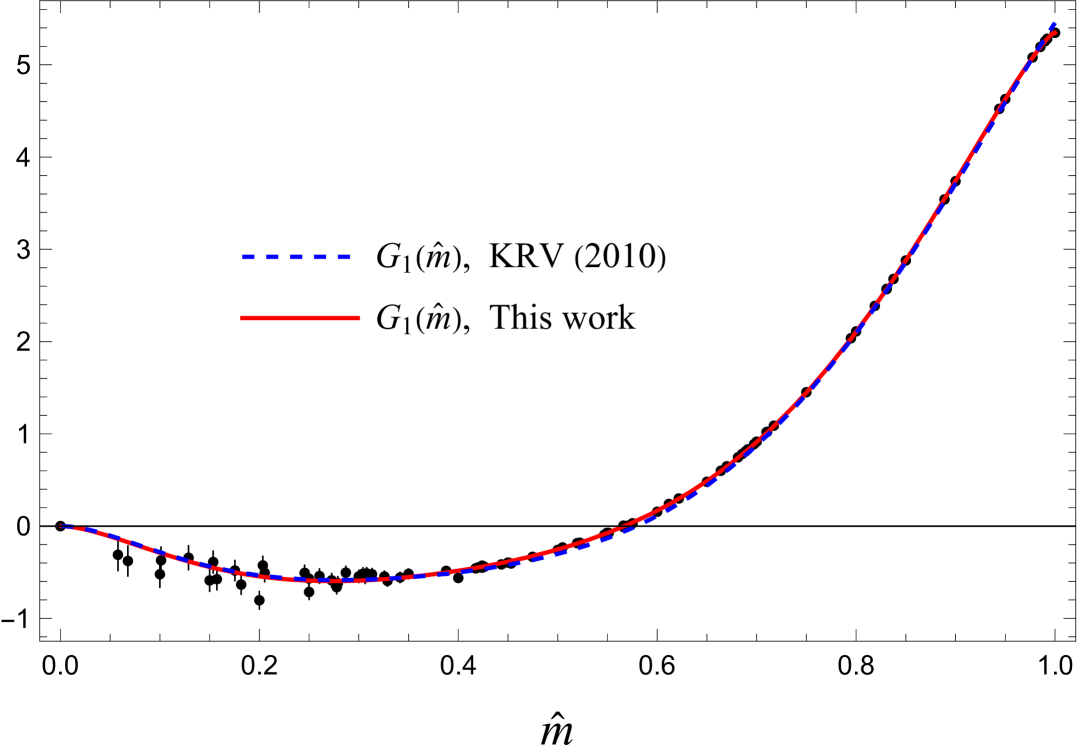
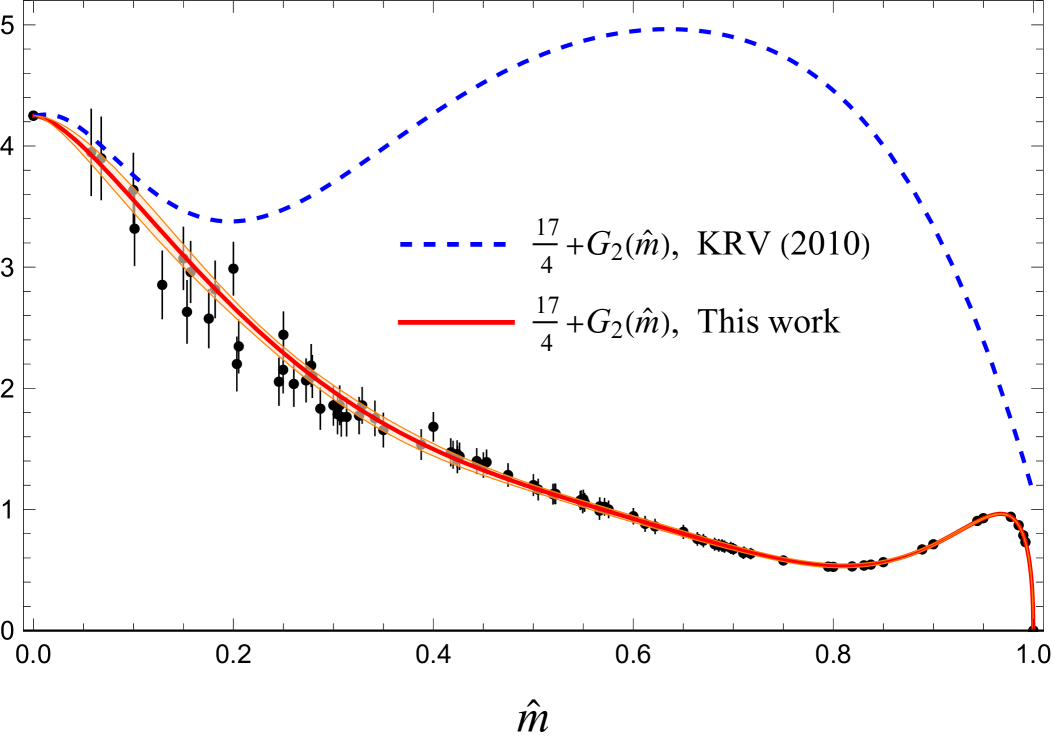
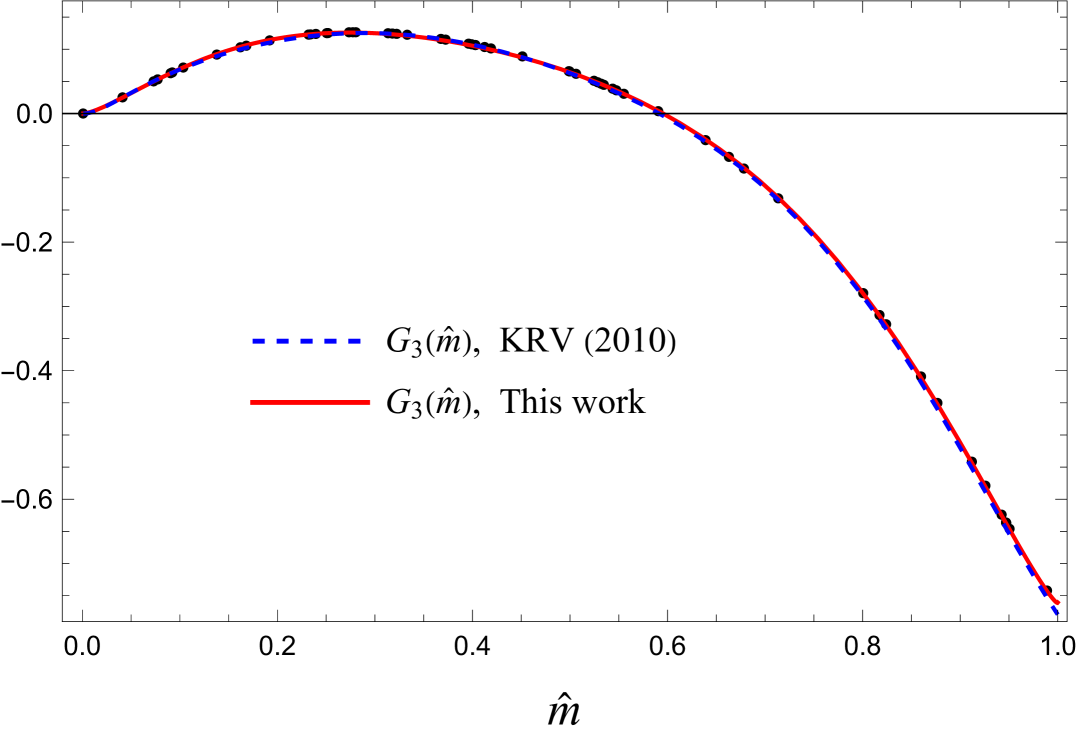
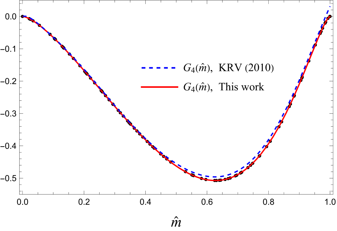
Figure 9: Comparison between the $G_{i}(\hat{m}=m/\mu)$ fitting functions from KRV (2010) Kurkela:2009gj and our reevaluated ones. The extra constant for $G_{2}$ is the one appearing in parenthesis in Eq.(8) such that its sum with $G_{2}$ must vanish for $\hat{m}\to 1$. The envelop shown for $G_{2}(\hat{m})$ represents 3-$\sigma$ confidence level of the obtained fit, given statistical errors of ${\cal O}(\leq 1\%)$ obtained for the relevant $I_{k}$ integral results.

According to Fig. 9, we thus obtain very good agreement for $G_{1}$, $G_{3}$, $G_{4}$, but sizable differences in $G_{2}(\hat{m})$ as compared to Kurkela:2009gj for intermediate and large $\hat{m}=m/\mu$ values. Notice also the vanishing of the $C_{F}$ contribution $17/4+G_{2}(\hat{m})\to 0$ for $\hat{m}\to 1$ in Fig. 9, as expected for $\mathcal{M}_{3}$ consistently from the fact that $p_{F}$ provides a cut-off for the momenta integration domain.

Appendix C non-diagonal massive NNLO contributions

C.1 Derivation of the NNLO non-diagonal $\mathcal{M}_{3}^{N_{f}=2^{*}+1^{*}}$ contribution

For the sake of clarity we stick to the same notations introduced in Kurkela:2009gj . The one-loop gluon polarization tensor is conveniently split into a vacuum ($T=\mu=0$) and matter contribution via

$$\Pi^{\mu\nu}(\vec{m}^{2},K) = \Pi_{\rm vac}^{\mu\nu}(\vec{m}^{2},K)+\Pi_{\rm mat}^{\mu\nu}(\vec{m}^{2},K),$$ (87)

where we suppressed the trivial color factor $\delta_{ab}$ and $\vec{m}^{2}$ means $(m_{i}^{2})_{i\in 1\dots N_{f}}$. Lorentz symmetry and gauge invariance give

$$\Pi^{\mu\nu}_{\rm vac}(\vec{m}^{2},K) = \Pi_{\rm vac}\left(\vec{m}^{2},K^{2}\right){\frac{g^{2}}{(4\pi)^{2}}\,}\left({\frac{\Lambda^{2}}{K^{2}}\,}\right)^{\!\!\varepsilon}\left(K_{\mu}K_{\nu}-K^{2}\delta_{\mu\nu}\right),$$ (88)

and a direct calculation leads to

$$\Pi_{\rm vac}\left(\vec{m}^{2},K^{2}\right) = \underbrace{-2^{5-2d}\pi^{\frac{7-d}{2}}(3d-2)C_{A}{\frac{{\rm csc}(\frac{\pi\,d}{2})}{\Gamma(\frac{d+1}{2})}\,}}_{f_{0}}-\sum_{j=1}^{N_{f}}2^{6-d}\pi^{\frac{4-d}{2}}\Gamma\left(\frac{4-d}{2}\right)\int_{0}^{1}{\rm d}x(x(1-x))^{\frac{d-2}{2}}\left(1+{\frac{m_{j}^{2}/K^{2}}{x(1-x)}\,}\right)^{\frac{d-4}{2}}$$ (89)

$$\equiv f_{0}+\sum_{j=1}^{N_{f}}f_{1}\left({\frac{m_{j}^{2}}{K^{2}}\,}\right).$$

To evaluate $\mathcal{M}_{3}^{N_{f}=2^{*}+1^{*}}$, we only need to modify the VM graph which only contributes to the 1-cut and 2-cut contributions. The expressions for the 2GI graphs derived in Kurkela:2009gj are

$$\frac{\Omega_{\rm 2GI}^{m,1c}(m_{i})}{V} = -d_{A}m_{i}^{2}\Bigg{\{}C_{A}\Bigg{[}\frac{16}{\varepsilon^{2}}+\frac{10}{3}\left(6\ln\frac{\Lambda}{m_{i}}+1\right)\frac{1}{\varepsilon}$$

$$- \left(4\ln\frac{\Lambda}{m_{i}}+\frac{136}{3}\right)\ln\frac{\Lambda}{m_{i}}-\frac{82}{3}+\pi^{2}\left(\frac{41}{6}-8\ln\,2\right)+12\zeta(3)\Bigg{]}I_{1}(m_{i})$$

$$+ C_{F}\Bigg{[}\bigg{\{}\frac{18}{\varepsilon^{2}}-\frac{3}{2\varepsilon}-6\left(12\ln\frac{\Lambda}{m_{i}}+5\right)\ln\frac{\Lambda}{m_{i}}-\frac{313}{4}$$

$$- \pi^{2}\left({\frac{35}{3}\,}-16\ln\,2\right)-24\zeta(3)\bigg{\}}I_{1}(m_{i})$$

$$+ m_{i}^{2}\bigg{\{}\frac{18}{\varepsilon^{2}}-36\left(2\ln{\frac{\Lambda}{m_{i}}\,}+\frac{8}{3}\right)\ln\frac{\Lambda}{m_{i}}-32\bigg{\}}I_{1b}(m_{i})\Bigg{]}$$

$$- N_{f}\Bigg{[}\frac{4}{\varepsilon^{2}}+8\bigg{(}\ln\frac{\Lambda}{m_{i}}+\frac{2}{3}\bigg{)}\frac{1}{\varepsilon}+8\left(\ln\frac{\Lambda}{m_{i}}+{\frac{4}{3}\,}\right)\ln\frac{\Lambda}{m_{i}}+{\frac{32}{3}\,}+\frac{\pi^{2}}{3}\Bigg{]}I_{1}(m_{i})\Bigg{\}}\,\frac{g^{4}({\Lambda})}{(4\pi)^{4}},$$

$${\frac{\Omega_{\rm 2GI}^{m,2c}(m_{i})}{V}\,} = -d_{A}\Bigg{\{}C_{A}\left[\left(\frac{5}{3}I_{1}(m_{i})^{2}-\frac{10}{3}m_{i}^{2}I_{2}(m_{i})\right)/\varepsilon+I_{10}(m_{i})+(-4I_{1}(m_{i})^{2}+8m_{i}^{2}I_{2}(m_{i}))\ln{\frac{\bar{\Lambda}}{m_{i}}\,}\right]$$ (91)

$$+ C_{F}\left[I_{11}(m_{i})+\left[24(m_{i}^{2}I_{2}(m_{i})-m_{i}^{2}I_{1b}(m_{i})I_{1}(m_{i})+2m_{i}^{4}I_{2b}(m_{i}))+48m_{i}^{4}I_{8}(m_{i})\right]\ln{\frac{\Lambda}{m_{i}}\,}\right]$$

$$+ N_{f}\Bigg{[}\left(-\frac{2}{3}I_{1}(m_{i})^{2}+\frac{4}{3}m_{i}^{2}I_{2}(m_{i})\right)/\varepsilon+\frac{2}{3}I_{1}(m_{i})^{2}\Bigg{]}\Bigg{\}}\,{\frac{g^{4}({\Lambda})}{(4\pi)^{2}}\,},$$

where the coupling $g$ and the quark mass $m_{i}$ are renormalized quantities. The divergences in the previous contributions cancel out with lowest order mass and coupling renormalization (see the discussion in Appendix A). There is no need to modify the $N_{f}$ coefficient depending on the case at hand ($N_{f}=2+1^{*},\ N_{f}=3^{*},\dots$) in the 2GI function since it only comes from renormalization.

C.2 Non-diagonal VV contribution

The “VV” additional contribution to the pressure, for arbitrary $m_{i},m_{j}$ different quark masses, may be derived from appropriately applying RG invariance properties with already known three-loop vacuum results from specific quantities, thus without need of actual three-loop calculations. More precisely, using results for the (quark sector) vacuum energy anomalous dimensionvacEn5l , and from the quark condensateKNcond ; KNcond2 , we can obtain the non-diagonal NNLO VV pressure contribution. The vacuum pressure given in Eq.(25) is normalized to one flavor of quark, but here it is more convenient to rewrite this contribution directly taking into account the $N_{f}\otimes N_{f}$ degrees of freedom. Using combinatorics, one finds:

$$N_{f}\,P^{v}_{\rm NNLO}(m,N_{h}=N_{f},N_{l}=0)\to P^{v}_{\rm NNLO}\equiv (N_{f}-1)P^{v,d}_{\rm NNLO}(m,N_{h}=N_{f}-1,N_{l}=1)$$ (93)

$$+P^{v,d}_{\rm NNLO}(m_{3},N_{h}=1,N_{l}=N_{f}-1)+2(N_{f}-1)P^{v,nd}_{\rm NNLO}(m,m_{3}),$$

with

$$P^{v,nd}_{\rm NNLO}(m,m_{3})= \frac{1}{\pi^{2}}\frac{g^{4}}{(4\pi)^{4}}m^{2}m_{3}^{2}\left(\alpha_{32}^{nd}(\ln\frac{m}{\Lambda}+\ln\frac{m_{3}}{\Lambda})+\alpha_{33}^{nd}\right)$$ (94)

$$\alpha_{32}^{nd}= -3N_{c}C_{F}T_{f}=-6,\;\;\;\alpha_{33}^{nd}=\frac{29}{3}-12\zeta(3).$$

In the diagonal part of the pressure, $N_{l}$ has been replaced by $N_{l}=N_{f}-N_{h}$ such that $N_{f}=N_{h}+N_{l}$ is always satisfied. As a crosscheck, for $m_{s}=0$, i.e, $m_{3}=m$, the right hand-side of Eq.(93) reproduces the left-hand side.

C.3 Non-diagonal VM contribution

Following Kurkela:2009gj , we re-evaluate the 1- and 2-cut contributions:

$$\begin{split}\frac{\Omega_{\rm VM}^{\rm m,1c}(m_{i})}{V}=&\ 2d_{A}\frac{g^{4}}{(4\pi)^{2}}\Lambda^{2\varepsilon}\Bigg{\{}2m_{i}^{2}\left(f_{0}\mathcal{D}_{4}\begin{pmatrix}m_{i}&m_{i}&0\\ c&1&1\end{pmatrix}+\sum_{j}^{N_{f}}\tilde{\mathcal{D}}_{4}\begin{pmatrix}m_{j}&\Big{\rvert}&m_{i}&m_{i}&0\\ \varepsilon&\Big{\rvert}&c&1&1\end{pmatrix}\right)\\ &-(1-\varepsilon)\left(f_{0}\mathcal{D}_{4}\begin{pmatrix}m_{i}&m_{i}&0\\ c&1&\varepsilon\end{pmatrix}+\sum_{j}^{N_{f}}\tilde{\mathcal{D}}_{4}\begin{pmatrix}m_{j}&\Big{\rvert}&m_{i}&m_{i}&0\\ \varepsilon&\Big{\rvert}&c&1&\varepsilon\end{pmatrix}\right)+(1-\varepsilon)\sum_{j}^{N_{f}}\tilde{\mathcal{D}}_{5}\begin{pmatrix}m_{j}&\Big{\rvert}&0\\ \varepsilon&\Big{\rvert}&1+\varepsilon\end{pmatrix}\Bigg{\}},\end{split}$$ (95)

$$\begin{split}\frac{\Omega_{\rm VM}^{\rm m,2c}(m_{i})}{V}=&-d_{A}\frac{g^{4}}{(4\pi)^{2}}\Lambda^{2\varepsilon}\Bigg{\{}2m_{i}^{2}\left(\frac{f_{0}}{((P-Q)^{2})^{1+\varepsilon}}+\frac{1}{(P-Q)^{2}}\sum_{j}^{N_{f}}\tilde{\mathcal{D}}_{4}\begin{pmatrix}m_{j}&\Big{\rvert}&m_{i}&m_{i}&0\\ \varepsilon&\Big{\rvert}&c&c&\varepsilon\end{pmatrix}\right)\hskip 62.59596pt\\ &-(1-\varepsilon)\left(\frac{f_{0}}{((P-Q)^{2})^{\varepsilon}}+\sum_{j}^{N_{f}}\tilde{\mathcal{D}}_{4}\begin{pmatrix}m_{j}&\Big{\rvert}&m_{i}&m_{i}&0\\ \varepsilon&\Big{\rvert}&c&c&\varepsilon\end{pmatrix}\right)\Bigg{\}},\end{split}$$ (96)

where $m_{j}$ is the mass of the quark flowing in the vacuum loop and $m_{i}$ the mass flowing in the matter loop. The tilde on the $D_{i}$ functions means that it is multiplied by $f_{1}(m_{j})$ prior to integration. For this calculation we needed to reevaluate the 1-cut $\mathcal{D}_{4}$ integrals whose expression are given in appendix C.4.
Once implemented in $\Omega_{\rm VM}$ we find:

$$\begin{split}\frac{\Omega_{\rm VM}^{m,1c}(m_{i})}{V}=&\frac{d_{A}m_{i}^{2}g^{4}I_{1}(m_{i})}{(4\pi)^{4}}\Bigg{\{}C_{A}\Bigg{[}\frac{5}{\varepsilon^{2}}+\frac{1}{\varepsilon}\left(20\ln\frac{\Lambda}{m_{i}}+\frac{39}{2}\right)+2\left(20\ln\frac{\Lambda}{m_{i}}+39\right)\ln\frac{\Lambda}{m_{i}}+\frac{261}{4}+\frac{25\pi^{2}}{6}\Bigg{]}-N_{f}\Bigg{[}\frac{2}{\varepsilon^{2}}+\frac{1}{\varepsilon}\left(7+8\ln\frac{\Lambda}{m_{i}}\right)\\ &+\frac{13}{2}+\frac{\pi^{2}}{3}+16\ln^{2}\frac{\Lambda}{m_{i}}+28\ln\frac{\Lambda}{m_{i}}\Bigg{]}-\sum_{j=1}^{N_{f}}\Bigg{[}4\left({\rm Li}_{2}(\nu_{ij})\left(1+\nu_{ij}^{-2}\right)-\frac{1}{\nu_{ij}^{2}}-\Phi(\nu_{ij},2,\frac{3}{2})(1+\nu_{ij})+\mathcal{F}(\nu_{ij})\right)\Bigg{]}\Bigg{\}},\\ &\mathcal{F}(\nu_{ij})=\ln\nu_{ij}\Bigg{\{}\ln(1-\nu_{ij})\left(1+\nu_{ij}^{-2}\right)+2\frac{{\rm Arctanh}(\sqrt{\nu_{ij}})}{\sqrt{\nu_{ij}}}(1+\nu_{ij}^{-1})-\nu_{ij}^{-1}-\frac{1}{2}\ln\nu_{ij}\Bigg{\}},\ \ \mathcal{F}(\nu_{ij}=1)=0,\end{split}$$ (97)

with $\nu_{ij}=(m_{i}/m_{j})^{2}$, and

$$\begin{split}\frac{\Omega_{\rm VM}^{m,2c}(m_{i})}{V}=&\frac{d_{A}g^{4}}{(4\pi)^{2}}\Bigg{\{}C_{A}\Bigg{[}\frac{1}{\varepsilon}\left(\frac{5}{3}I_{1}(m_{i})^{2}-\frac{10}{3}m_{i}^{2}I_{2}(m_{i})\right)+\left(\frac{10}{3}I_{1}(m_{i})^{2}-\frac{20}{3}m_{i}^{2}I_{2}(m_{i})\right)\ln\frac{\Lambda}{m_{i}}+\frac{16}{9}I_{1}(m_{i})^{2}-\frac{62}{9}m_{i}^{2}I_{2}(m_{i})\\ &-\frac{5}{3}I_{1c}(m_{i})+\frac{10}{3}m_{i}^{2}I_{2c}(m_{i})\Bigg{]}-N_{f}\Bigg{[}\frac{1}{\varepsilon}\left(\frac{2}{3}I_{1}(m_{i})^{2}-\frac{4}{3}m_{i}^{2}I_{2}(m_{i})\right)+\left(\frac{4}{3}I_{1}(m_{i})^{2}-\frac{8}{3}m_{i}^{2}I_{2}(m_{i})\right)\ln\frac{\Lambda}{m_{i}}\\ &+\frac{4}{9}I_{1}(m_{i})^{2}-\frac{20}{9}m_{i}^{2}I_{2}(m_{i})-\frac{2}{3}I_{1c}(m_{i})+\frac{4}{3}m_{i}^{2}I_{2c}(m_{i})\Bigg{]}+\frac{2}{3}\sum_{j=1}^{N_{f}}I_{12}^{\rm bis}(m_{i},\nu_{ij})\Bigg{\}},\end{split}$$ (98)

C.4 Unequal mass integrals

Finally additional ingredients needed for our generalization to unequal quark masses, entering Eq.(98), are

$$I_{12}^{\rm bis}(\hat{m}_{i},\nu_{ij})= \int_{p}\int_{q}\left(\frac{a_{i}-2}{a_{i}^{2}\,\nu_{ij}}\right)\left(4-a_{i}\,\nu_{ij}\ln(a_{i}\,\nu_{ij})+2(a_{i}\,\nu_{ij}-2)\sqrt{\frac{4+a_{i}\,\nu_{ij}}{a_{i}\,\nu_{ij}}}{\rm Arctanh}\left[\sqrt{\frac{a_{i}\,\nu_{ij}}{4+a_{i}\,\nu_{ij}}}\right]\right),\ \ a_{i}=\frac{\left(P-Q\right)^{2}}{m_{i}^{2}}$$ (99)

$$=\ \hat{m}^{2}\hat{u}^{2}\Bigg{\{} -3.459417+0.421797\hat{m}^{2}-0.776318\hat{u}-0.770475\hat{u}^{3}+(0.387893+2.123092\hat{m})\nu_{ij}$$

$$+(0.181022-0.506166\hat{m}+0.139366\hat{m}^{2})\nu_{ij}^{2}+(0.664467+0.115689\hat{m}+0.115689\ln\hat{m})/(\hat{m}\ \nu_{ij})$$

$$+(1.960279-3.332848\hat{m})\ln\nu_{ij}+(-0.585635-0.680364\hat{m}+0.576210\ln\hat{m})\ln^{2}\nu_{ij}\Bigg{\}}.$$

Note that the 2-dimensional fit of $I_{12}^{\rm bis}(\hat{m}_{i},\nu_{ij})$ is only valid (within $\sim 1\%$ accuracy) in the region $x\otimes\nu_{ij}\in[0,1]\otimes[0.4,2.5]$, where the latter range is largely sufficient for physically relevant values of $\nu_{ij}$.
The last ingredients required to generalize the “VM” contribution for the $N_{f}=2^{*}+1^{*}$ case are the vacuum amplitude $\tilde{D}_{i}$, defined in Fig. 12 in Kurkela:2009gj and obtained from Di_Ref . These functions correspond to different scalar Feynman graph topologies, where an upper index indicate the mass of the propagator and the lower index indicates the power of the propagator. For tilde functions, the first dual arguments (before the vertical line) indicates the propagator coming from the multiplication of $f_{1}$ prior to integration :

$$\mathcal{D}_{4}= \ \leavevmode\hbox to45.92pt{\vbox to45.92pt{\text{[drawing]}}}\ \ ,\ \ \ \mathcal{D}_{5}=\leavevmode\hbox to40.23pt{\vbox to40.23pt{\text{[drawing]}}} (0,0.9) (0,-0.9)$$ (100)

$$\mathcal{D}_{4}\begin{pmatrix}m_{1}&m_{2}&0\\ \alpha&\beta&\gamma\end{pmatrix}=\int_{-\infty+i\mu}^{\infty+i\mu}dp_{0}\int\frac{d^{d-1}p}{\left(2\pi\right)^{d-1}} \int_{-\infty+i\mu}^{\infty+i\mu}dq_{0}\int\frac{d^{d-1}q}{\left(2\pi\right)^{d-1}}\frac{1}{\left(p_{0}^{2}+p^{2}+m_{1}^{2}\right)^{\alpha}\left(q_{0}^{2}+q^{2}+m_{2}^{2}\right)^{\beta}\left((p_{0}-q_{0})^{2}+(p-q)^{2}\right)^{\gamma}}.$$

For the relevant $D_{i}$ function we use dimensional regularization where the integration measure reads:

$$\int_{P}=\left(\frac{\Lambda^{2}e^{\gamma}}{4\pi}\right)^{\varepsilon}\int\frac{d^{d}P}{(2\pi)^{d}},\ \ \ \int_{\vec{p}}=\left(\frac{\Lambda^{2}e^{\gamma}}{4\pi}\right)^{\varepsilon}\int\frac{d^{d-1}\vec{p}}{(2\pi)^{d-1}},\ \ \ d=4-2\varepsilon,$$ (101)

where $P$ is an Euclidean momentum and $\gamma$ is Euler’s constant. On top of that, a “$c$” lower index indicates that the corresponding propagator has been cut following the rules explained in section II.A.2.
Finally, the $\tilde{\mathcal{D}_{i}}$ which required re-evaluation when using two different masses, reads

$$\begin{split}&\left(\frac{\Lambda^{2}e^{\gamma}}{4\pi}\right)^{\varepsilon}\tilde{\mathcal{D}}_{4}\begin{pmatrix}m_{j}&\Big{\rvert}&m_{i}&m_{i}&0\\ \varepsilon&\Big{\rvert}&c&1&1+\varepsilon\end{pmatrix}=-\frac{1}{3(4\pi)^{2}}\left(\frac{\Lambda^{2}}{m_{i}\ m_{j}}\right)^{2\varepsilon}\Bigg{\{}\frac{1}{\varepsilon^{2}}+\frac{1}{\varepsilon}\left(\frac{14}{3}-\ln\nu_{ij}\right)+(1-3\nu_{ij})\Phi(\nu_{ij},2,\frac{3}{2})+\frac{46}{9}+\frac{\pi^{2}}{6}\\ &\hskip 113.81102pt+\frac{2}{3}\ln\nu_{ij}\Bigg{(}-7+3\nu_{ij}^{-1}+\nu_{ij}^{-\frac{1}{2}}(9-3\nu_{ij}^{-1}){\rm Arctanh}(\sqrt{\nu_{ij}})+3\ln(1-\nu_{ij})\Bigg{)}+2{\rm Li}_{2}(\nu_{ij})\Bigg{\}}\\ &\left(\frac{\Lambda^{2}e^{\gamma}}{4\pi}\right)^{\varepsilon}\tilde{\mathcal{D}}_{4}\begin{pmatrix}m_{j}&\Big{\rvert}&m_{i}&m_{i}&0\\ \varepsilon&\Big{\rvert}&c&1&\varepsilon\end{pmatrix}=\frac{m_{i}^{2}}{3(4\pi)^{2}}\left(\frac{\Lambda^{2}}{m_{i}\ m_{j}}\right)^{2\varepsilon}\Bigg{\{}\frac{1}{\varepsilon^{2}}+\frac{1}{\varepsilon}\left(\frac{13}{6}+6\nu_{ij}^{-\frac{1}{2}}-\ln\nu_{ij}\right)-\frac{67}{36}+\frac{\pi^{2}}{6}-8\,\nu_{ij}\Phi(\nu_{ij},2,\frac{5}{2})\\ &\hskip 56.9055pt+\frac{1}{2}\ln(\nu_{ij})\left(-\frac{13}{3}-\frac{8}{\nu_{ij}}-\ln(\nu_{ij})+\frac{32}{(\sqrt{\nu_{ij}})^{3}}{\rm Arctanh}(\sqrt{\nu_{ij}})+\left(4+\frac{12}{\nu_{ij}^{2}}\right)\ln(1-\nu_{ij})\right)+\left(2+\frac{6}{\nu_{ij}^{2}}\right){\rm Li}_{2}(\nu_{ij})\Bigg{\}}.\end{split}$$ (102)

For this calculation we used Mellin-Barnes techniques to perform the integration over the Feynman parameters (see for instance Smirnov:2012gma for a review). In practise, it amounts to factorize the mass dependence of the propagator coming from $f_{1}$ in $\tilde{\mathcal{D}}_{4}$ into:

$$\left(1+\frac{m^{2}}{(P-Q)^{2}x(1-x)}\right)^{-\varepsilon}=\frac{1}{2\pi i}\oint ds\,\Gamma(-s)\Gamma(s+\varepsilon)\left(\frac{m^{2}}{\left(P-Q\right)^{2}\,x(1-x)}\right)^{s},$$ (103)

where $x$ is a Feynman parameter. Such factorization makes the integration over all Feynman parameters straightforward in terms of $\Gamma$ functions, then the remaining $s$-integral is carried out via the Residue theorem with appropriately chosen contours.

References

• (1) J. P. Blaizot, E. Iancu and A. Rebhan, In *Hwa, R.C. (ed.) et al.: Quark gluon plasma* 60-122 [hep-ph/0303185]; U. Kraemmer and A. Rebhan, Rept. Prog. Phys.  67, 351 (2004) [arXiv:hep-ph/0310337 [hep-ph]]; J. Ghiglieri, A. Kurkela, M. Strickland and A. Vuorinen, Phys. Rept. 880, 1 (2020) [arXiv:2002.10188 [hep-ph]].
• (2) Y. Aoki, G. Endrodi, Z. Fodor, S. D. Katz and K. K. Szabo, Nature 443, 675-678 (2006) [arXiv:hep-lat/0611014 [hep-lat]]; Y. Aoki, S. Borsanyi, S. Durr, Z. Fodor, S. D. Katz, S. Krieg and K. K. Szabo, JHEP 06, 088 (2009) [arXiv:0903.4155 [hep-lat]]; S. Borsanyi et al. [Wuppertal-Budapest], JHEP 09, 073 (2010) [arXiv:1005.3508 [hep-lat]]; A. Bazavov, T. Bhattacharya, M. Cheng, C. DeTar, H. T. Ding, S. Gottlieb, R. Gupta, P. Hegde, U. M. Heller and F. Karsch, et al. Phys. Rev. D 85, 054503 (2012) [arXiv:1111.1710 [hep-lat]].
• (3) P. de Forcrand, PoS LAT 2009, 010 (2009); [arXiv:1005.0539 [hep-lat]]; G. Aarts, J. Phys. Conf. Ser.  706, 022004 (2016). [arXiv:1512.05145 [hep-lat]].
• (4) K. Hebeler, Phys. Rept. 890, 1-116 (2021) [arXiv:2002.09548 [nucl-th]].
• (5) C. Drischler, K. Hebeler and A. Schwenk, Phys. Rev. Lett. 122, no.4, 042501 (2019) [arXiv:1710.08220 [nucl-th]].
• (6) G. Baym, T. Hatsuda, T. Kojo, P. D. Powell, Y. Song and T. Takatsuka, Rept. Prog. Phys. 81, no.5, 056902 (2018) [arXiv:1707.04966 [astro-ph.HE]].
• (7) E. Annala, T. Gorda, A. Kurkela, J. Nättilä and A. Vuorinen, Nature Phys. 16, no.9, 907-910 (2020) [arXiv:1903.09121 [astro-ph.HE]].
• (8) O. Komoltsev and A. Kurkela, Phys. Rev. Lett. 128, no.20, 202701 (2022) [arXiv:2111.05350 [nucl-th]].
• (9) E. Annala, T. Gorda, J. Hirvonen, O. Komoltsev, A. Kurkela, J. Nättilä and A. Vuorinen, Nature Commun. 14, no.1, 8451 (2023) [arXiv:2303.11356 [astro-ph.HE]].
• (10) O. Komoltsev, R. Somasundaram, T. Gorda, A. Kurkela, J. Margueron and I. Tews, Phys. Rev. D 109, no.9, 094030 (2024) [arXiv:2312.14127 [nucl-th]].
• (11) S. Gupta, X. Luo, B. Mohanty, H. G. Ritter and N. Xu, Science 332, 1525-1528 (2011) [arXiv:1105.3934 [hep-ph]].
• (12) B. Friman, C. Hohne, J. Knoll, S. Leupold, J. Randrup, R. Rapp and P. Senger, Lect. Notes Phys. 814, pp.1-980 (2011) doi:10.1007/978-3-642-13293-3
• (13) T. Ablyazimov et al. [CBM], Eur. Phys. J. A 53, no.3, 60 (2017) [arXiv:1607.01487 [nucl-ex]].
• (14) A. D. Linde, Phys. Lett. B 96, 289-292 (1980)
• (15) B. A. Freedman and L. D. McLerran, Phys. Rev. D 16,1147 (1977); Phys. Rev. D 16,1169 (1977).
• (16) E. S. Fraga and P. Romatschke, Phys. Rev. D 71, 105014 (2005) [arXiv:hep-ph/0412298 [hep-ph]].
• (17) M. Laine and Y. Schröder, Phys. Rev. D 73, 085009 (2006). [arXiv:hep-ph/0603048 [hep-ph]].
• (18) A. Kurkela, P. Romatschke and A. Vuorinen, Phys. Rev. D 81, 105021 (2010) [arXiv:0912.1856 [hep-ph]].
• (19) T. Graf, J. Schaffner-Bielich and E. S. Fraga, Eur. Phys. J. A 52, no.7, 208 (2016) [arXiv:1507.08941 [hep-ph]].
• (20) A. Ipp, K. Kajantie, A. Rebhan and A. Vuorinen, Phys. Rev. D 74, 045016 (2006) doi:10.1103/PhysRevD.74.045016 [arXiv:hep-ph/0604060 [hep-ph]].
• (21) A. Kurkela and A. Vuorinen, Phys. Rev. Lett. 117, no.4, 042501 (2016) doi:10.1103/PhysRevLett.117.042501 [arXiv:1603.00750 [hep-ph]].
• (22) R. R. Parwani, Phys. Rev. D 45, 4695 (1992) [erratum: Phys. Rev. D 48, 5965 (1993)] [arXiv:hep-ph/9204216 [hep-ph]]; F. Karsch, A. Patkos and P. Petreczky, Phys. Lett. B 401, 69 (1997) [arXiv:hep-ph/9702376 [hep-ph]].
• (23) J. O. Andersen, E. Braaten and M. Strickland, Phys. Rev. D 63, 105008 (2001); [arXiv:hep-ph/0007159 [hep-ph]].
• (24) J. O. Andersen, E. Braaten and M. Strickland, Phys. Rev. Lett.  83, 2139 (1999); [hep-ph/9902327]. J. O. Andersen, E. Braaten and M. Strickland, Phys. Rev. D 61, 074016 (2000) [arXiv:hep-ph/9908323 [hep-ph]].
• (25) E. Braaten and R. D. Pisarski, Phys. Rev. D 45, 1827 (1992).
• (26) J. O. Andersen, E. Braaten, E. Petitgirard and M. Strickland, Phys. Rev. D 66, 085016 (2002) [arXiv:hep-ph/0205085 [hep-ph]].
• (27) N. Haque, M. G. Mustafa and M. Strickland, Phys. Rev. D 87, no.10, 105007 (2013) [arXiv:1212.1797 [hep-ph]].
• (28) J. O. Andersen, L. E. Leganger, M. Strickland and N. Su, JHEP 1108, 053 (2011) [arXiv:1103.2528 [hep-ph]]; N. Haque, A. Bandyopadhyay, J. O. Andersen, M. G. Mustafa, M. Strickland and N. Su, JHEP 1405, 027 (2014); [arXiv:1402.6907 [hep-ph]]; S. Mogliacci, J. O. Andersen, M. Strickland, N. Su and A. Vuorinen, JHEP 1312, 055 (2013); [arXiv:1307.8098 [hep-ph]].
• (29) T. Gorda, A. Kurkela, P. Romatschke, M. Säppi and A. Vuorinen, Phys. Rev. Lett. 121, no.20, 202701 (2018) [arXiv:1807.04120 [hep-ph]].
• (30) T. Gorda, A. Kurkela, R. Paatelainen, S. Säppi and A. Vuorinen, Phys. Rev. Lett. 127, no.16, 162003 (2021) [arXiv:2103.05658 [hep-ph]].
• (31) T. Gorda, A. Kurkela, R. Paatelainen, S. Säppi and A. Vuorinen, Phys. Rev. D 104, no.7, 074015 (2021) [arXiv:2103.07427 [hep-ph]].
• (32) T. Gorda, R. Paatelainen, S. Säppi and K. Seppänen, Phys. Rev. Lett. 131, no.18, 181902 (2023) [arXiv:2307.08734 [hep-ph]].
• (33) L. Fernandez and J. L. Kneur, Phys. Rev. Lett. 129, no.21, 212001 (2022) [arXiv:2109.02410 [hep-ph]].
• (34) J. L. Kneur and A. Neveu, Phys. Rev. D 88, no.7, 074025 (2013) [arXiv:1305.6910 [hep-ph]].
• (35) P.M. Stevenson, Phys. Rev. D 23, 2916 (1981); Nucl. Phys. B 203, 472 (1982).
• (36) R. Seznec and J. Zinn-Justin, J. Math. Phys. 20, 1398 (1979); J.C. Le Guillou and J. Zinn-Justin, Ann. Phys. 147, 57 (1983); J. Zinn-Justin, [arXiv:1001.0675 [math-ph]].
• (37) V.I. Yukalov, Theor. Math. Phys. 28, 652 (1976); W.E. Caswell, Ann. Phys. (N.Y) 123, 153 (1979); I.G. Halliday and P. Suranyi, Phys. Lett. B85, 421 (1979); R.P. Feynman and H. Kleinert, Phys. Rev. A34, 5080 (1986); A. Duncan and M. Moshe, Phys. Lett. B 215, 352-358 (1988) H.F. Jones and M. Moshe, Phys. Lett. B234, 492 (1990); A. Neveu, Nucl. Phys. B, Proc. Suppl. B18, 242 (1991); V. Yukalov, J. Math. Phys (N.Y) 32, 1235 (1991); S. Gandhi, H.F. Jones and M. Pinto, Nucl. Phys. B359, 429 (1991); C. M. Bender et al., Phys. Rev. D45, 1248 (1992); H. Yamada, Z. Phys. C59, 67 (1993); A.N. Sisakian, I.L. Solovtsov and O.P. Solovtsova, Phys. Lett. B321, 381 (1994); R. Guida, K. Konishi, and H. Suzuki, Ann. Phys. (N.Y.) 241, 152 (1995); 249, 109 (1996); H. Kleinert, Phys. Rev. D57, 2264 (1998); Phys. Lett. B434, 74 (1998).
• (38) S. Chiku and T. Hatsuda, Phys. Rev. D 58, 076001 (1998) [arXiv:hep-ph/9803226 [hep-ph]].
• (39) J. L. Kneur and A. Neveu, Phys. Rev. D 92, no.7, 074027 (2015) [arXiv:1506.07506 [hep-ph]].
• (40) J. L. Kneur and A. Neveu, Phys. Rev. D 101, no.7, 074009 (2020) [arXiv:2001.11670 [hep-ph]].
• (41) J. L. Kneur and M. B. Pinto, Phys. Rev. Lett.  116, 031601 (2016) [arXiv:1507.03508 [hep-ph]]; ibid, Phys. Rev. D 92, 116008 (2015) [arXiv:1508.02610 [hep-ph]].
• (42) L. Fernandez and J. L. Kneur, Phys. Rev. D 104, no.9, 096012 (2021) [arXiv:2107.13328 [hep-ph]].
• (43) J. L. Kneur, M. B. Pinto and T. E. Restrepo, Phys. Rev. D 104, no.3, 034003 (2021) [arXiv:2101.08240 [hep-ph]]; Phys. Rev. D 104, no.3, L031502 (2021) [arXiv:2101.02124 [hep-ph]].
• (44) J. L. Kneur, M. B. Pinto and T. E. Restrepo, Phys. Rev. D 100, 114006 (2019) [arXiv:1908.08363 [hep-ph]].
• (45) Supplementary material for Ref.Kurkela:2009gj can be found at http://hep.itp.tuwien.ac.at/~paulrom/eost0/eospaper.html
• (46) A. Vuorinen, Phys. Rev. D 68, 054017 (2003). [arXiv:hep-ph/0305183 [hep-ph]].
• (47) I. Ghisoiu, T. Gorda, A. Kurkela, P. Romatschke, S. Säppi and A. Vuorinen, Nucl. Phys. B 915, 102-118 (2017) [arXiv:1609.04339 [hep-ph]].
• (48) M. Tanabashi et al. [Particle Data Group], Phys. Rev. D 98, 030001 (2018).
• (49) A. Bazavov, N. Brambilla, X. Garcia Tormo, i, P. Petreczky, J. Soto and A. Vairo, Phys. Rev. D 86, 114031 (2012) [arXiv:1205.6155 [hep-ph]].
• (50) E. S. Fraga, A. Kurkela and A. Vuorinen, Astrophys. J. Lett. 781, no.2, L25 (2014) [arXiv:1311.5154 [nucl-th]].
• (51) V. P. Spiridonov and K. G. Chetyrkin, Sov. J. Nucl. Phys. 47 (1988), 522-527.
• (52) K. G. Chetyrkin and J. H. Kuhn, Nucl. Phys. B 432, 337-350 (1994), [arXiv:hep-ph/9406299 [hep-ph]].
• (53) B. M. Kastening, Phys. Rev. D 54, 3965-3975 (1996) [arXiv:hep-ph/9604311 [hep-ph]].
• (54) P. A. Baikov and K. G. Chetyrkin, PoS RADCOR2017, 025 (2018)
• (55) J. C. Collins, Renormalization, Cambridge University Press, Cambridge, England, 1984.
• (56) G. P. Lepage, J. Comput. Phys. 439, 110386 (2021) [arXiv:2009.05112 [physics.comp-ph]].
• (57) T. Hahn, Comput. Phys. Commun. 168, 78-95 (2005) [arXiv:hep-ph/0404043 [hep-ph]].
• (58) R. Bonciani et al., Nucl. Phys. B681, 261 (2004); B702 364(E) (2004); [arXiv:hep-ph/0310333 [hep-ph]]; R. Bonciani, P. Mastrolia, and E. Remiddi, Nucl. Phys. B690, 138 (2004) [arXiv:hep-ph/0311145 [hep-ph]]; Y. Schröder and A. Vuorinen, JHEP 06, 051 (2005) [arXiv:hep-ph/0503209 [hep-ph]]; S. Laporta and E. Remiddi, Nucl. Phys. B 704, 349-386 (2005) [arXiv:hep-ph/0406160 [hep-ph]].
• (59) V. A. Smirnov, “Analytic tools for Feynman integrals,” Springer Tracts Mod. Phys. 250 (2012), 1-296