Eigen-Cluster VIS: Improving Weakly-supervised Video Instance Segmentation by Leveraging Spatio-temporal Consistency

Abstract

The performance of Video Instance Segmentation (VIS) methods has improved significantly with the advent of transformer networks. However, these networks often face challenges in training due to the high annotation cost. To address this, unsupervised and weakly-supervised methods have been developed to reduce the dependency on annotations. This work introduces a novel weakly-supervised method called Eigen-cluster VIS that, without requiring any mask annotations, achieves competitive accuracy compared to other VIS approaches. This method is based on two key innovations: a Temporal Eigenvalue Loss (TEL) and a clip-level Quality Cluster Coefficient (QCC). The TEL ensures temporal coherence by leveraging the eigenvalues of the Laplacian matrix derived from graph adjacency matrices. By minimizing the mean absolute error (MAE) between the eigenvalues of adjacent frames, this loss function promotes smooth transitions and stable segmentation boundaries over time, reducing temporal discontinuities and improving overall segmentation quality. The QCC employs the K-means method to ensure the quality of spatio-temporal clusters without relying on ground truth masks. Using the Davies-Bouldin score, the QCC provides an unsupervised measure of feature discrimination, allowing the model to self-evaluate and adapt to varying object distributions, enhancing robustness during the testing phase. These enhancements are computationally efficient and straightforward, offering significant performance gains without additional annotated data. The proposed Eigen-Cluster VIS method is evaluated on the YouTube-VIS 2019/2021 and OVIS datasets, demonstrating that it effectively narrows the performance gap between the fully-supervised and weakly-supervised VIS approaches. The code is available on: https://github.com/farnooshar/EigenClusterVIS

I Introduction

Multi-object tracking and segmentation are two fundamental tasks in the field of computer vision with vast applications in areas like autonomous driving [1], surveillance [2], and sports analysis [3, 4]. Video Instance Segmentation [5], on the other hand, involves both segmenting and tracking instances across all video frames. Despite its challenging nature, there has been rapid progress in deep learning-based methods for this task, thanks to the availability of annotated datasets for the VIS [5, 6]. Although fully supervised methods have achieved considerable performance on these datasets, annotating many videos for this task is heavily labor-intensive and limits the dataset to a limited number of domains and classes. Specifically, this is an important problem for transformer-based VIS models [7, 8, 9], which are supposed to be very data-hungry to achieve their best performance.

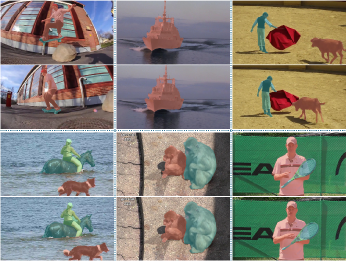
Figure 1: Visualization of Eigen-Cluster VIS Predictions. Eigen-Cluster VIS uses no video or image mask annotations, and achieves 44% mask AP on the YouTube-VIS 2019 validation dataset, with a ResNet-50 backbone. These outputs validate the fact that high performance VIS can be obtained without any mask annotations.

To address the aforementioned challenges, a various weakly-supervised [10, 11, 12, 13, 14] and unsupervised[15, 16, 17] methods have been proposed with different kinds of supervisions. Some methods rely on classification labels [18, 19] and use the optical flow [20, 21] methods for one-to-one correspondence. But, this kind of supervision is not sufficient for achieving higher performance. On the other hand, a variety of box-supervised methods have been proposed for image-level instance segmentation [22, 23, 24, 25, 26]. Although those methods achieve great performance due to the existence of large-scale datasets, like COCO [27], they are not completely appropriate for VIS, as they ignore the temporal information in videos. As such, their performance is lower when applied to the video. In fact, with a 3D spatio-temporal volume, some temporal consistency constraints can be utilized to improve the performance further. Recently, the MaskFree VIS [28] work proposed the first VIS method with bounding box supervision by applying temporal consistency loss to match patch-oriented one-to-many correspondences to handle the occlusion and homogenous region scenarios. Doing this reduces the gap between fully supervised and weakly supervised VIS.

In this work, we extend the idea of [28] and define two more temporal consistency constraints. Inspired by deep spectral methods [29], we leverage eigenvalues derived from the Laplacian matrix of a graph adjacency matrix as a robust representation of structural and spatial properties. To do this, first, a Temporal Eigenvalue Loss (TEL) is defined as clip-oriented and aims at minimizing the difference between the eigenvalues of instances in consecutive frames. This regularization term reduces the temporal discontinuities and improves the overall quality and reliability of the segmentation output for more consistent and visually pleasing results. This loss function integrates easily into existing VIS methods without requiring additional network parameters. Furthermore, a Quality Cluster Coefficient (QCC) is proposed for clip-level spatio-temporal consistency without relying on ground-truth labels. The proposed QCC measures the quality and discrimination power of dense spatio-temporal areas, enabling dynamic adjustment of the impact of both patch-oriented and clip-oriented constraints. Qualitative results are provided in Figure 1. To summarize, the main contributions of this work are as follows:

• Proposing a wealy-supervised VIS method called Eigen-cluster VIS, which only needs weak supervision to achieve competitive accuracy without requiring mask annotations. Notably, this method dose not add any trainable parameters to the network.

• Introducing clip-oriented views beside patch-oriented views to ensure spatio-temporal consistency with QCC and TEL. The QCC uses K-means clustering and the Davies-Bouldin score for unsupervised feature discrimination, while the TEL ensures temporal coherence by minimizing the MAE between eigenvalues of adjacent frames. Together, these functions enhance the overall performance of the proposed VIS method.

• Analyzing the effectiveness of the proposed method on the YouTube-VIS 2019/2021 and OVIS benchmarks, demonstrating that Eigen-cluster VIS narrows the performance gap between fully-supervised and weakly-supervised VIS methods.

II RELATED WORK

II-A Video Instance Segmentation

Based on their application, existing VIS methods can be divided into two distinct categories: offline and online methods.

II-A1 Online VIS

Online VIS methods [30, 31, 32, 33, 34, 35, 36] have made significant progress due to the availability of robust detectors and image-level instance segmentation methods. Most of those works, including [5] as the first VIS method, attempt to extend segmentation models [37, 38] by adding a tracking head. Due to their online nature, they can be applied to real-time scenarios such as video surveillance and autonomous driving.

II-A2 Offline VIS

Offline VIS methods [39, 40, 41, 42, 43], on the other hand, by having access to all frames, can take advantage of temporal information and post-processing, making them suitable for applications such as video editing and content analysis. The STEm-Seg [44], as one of the first offline VIS methods, uses clustering to track instances by viewing the input video as a spatio-temporal 3D volume.

Aside from the offline/online nature of VIS methods, transformer-based methods have recently emerged and achieved impressive results in this task [45, 46, 47, 48]. The [7] work was one of the first to employ transformers for VIS. Other methods like Seqformer [8] and Mask2Former [9] introduced the frame query decomposition and masked attention, respectively. The IDOL [49], while effective, relied on post-processing for tracking. Recent advancements, such as VITA [50] and DVIS [51], take a more sophisticated approach. The VITA leverages temporal interactions between the frame-level object queries, and DVIS adopts a modular design, separating VIS into distinct stages of segmentation, tracking, and refinement.

II-B Mask-Free Video Instance Segmentation

Existing weakly-supervised methods for mask-free instance segmentation primarily operate at image level [10, 23, 24, 11, 25, 26]. Early works, such as [52, 22], relied on region proposals, leading to slow training times. More recently, point-supervised instance segmentation methods have emerged [12, 13]. The BoxTeacher [53] work leverages a sophisticated teacher model to generate high-quality masks as pseudo-labels. While these methods demonstrate promising performance in weakly-supervised instance segmentation, they ignore temporal information presented in videos, as they operate solely at the image level.

Several works have been conducted in the areas of weakly-, semi-, and unsupervised VIS. Methods like flowIRN [19] leverage classification labels alongside optical flow to enforce temporal mask consistency, while Cluster2Former [14] utilizes scribble-based annotations. The SOLO-Track [54] proposes a novel semi-supervised method for VIS that requires no video annotations, and MinVIS [55] utilizes a small subset of annotated frames to train a query-based instance segmentation model with bipartite matching for mask tracking. In the unsupervised setting, VideoCutLER [16] employs MaskCut [15] to generate object pseudo-masks. It proposes ImageCut2Video to create synthetic videos using a pair of images and then trains an unsupervised VIS model using these mask trajectories. The most recent work, UVIS [17], uses DINO [56] for mask generation and leverages CLIP [57] to add semantic information to these masks. It then trains a transformer to learn queries for predicting per-frame instance masks and introduces tracking banks to associate masks between frames.

The most relevant methods related to this work are Mask-Free VIS [28] and PM-VIS [58]. The Mask-Free VIS incorporates [24] as its instance segmentation baseline and introduces a novel temporal consistency constraint called Temporal KNN-patch Loss. This constraint is achieved by finding one-to-many patch matches across frames followed by k-nearest neighbor selection. A consistency loss is then applied to these matched patches. On the other hand, the PM-VIS employs different methods to generate three distinct pseudo-masks, which are filtered to achieve high-quality pseudo-masks. Finally, a fully-supervised VIS method is trained on these filtered pseudo-masks.

II-C Deep Spectral Methods

The spectral graph theory, initially introduced in [59], has evolved to connect global graph features by the eigenvalues and eigenvectors of the Laplacian matrix [60, 61]. Notably, [60] proposed the Fidler eigenvalue, the second smallest eigenvalue, as a measure of graph connectivity. Furthermore, [61] demonstrated the use of graph Laplacian eigenvectors for achieving energy-minimizing graph partitions. With the advent of machine learning and computer vision, [62] and [63] pioneered the application of spectral clustering for image segmentation. Inspired by these works, a recent method like DSM [29] and [64], leverage features extracted from a self-supervised transformer-based backbone, along with the Laplacian of the affinity matrix and patch-wise similarities, to perform tasks such as object localization and semantic segmentation.

Building upon DSM [29], research has primarily focused on object localization [64, 65, 15], semantic segmentation [66, 67, 68], and video object segmentation [69, 70, 71]. In contrast, instance segmentation has received less attention. The MaskCut [15] method constructs a patch-wise similarity matrix by using a self-supervised backbone. It then iteratively applies Normalized Cuts to generate foreground masks and masking out affinity matrix values for each discovered object. The work in [72] has a similar paradigm to the DSM and shows that not all channels of a self-supervised backbone are useful for instance segmentation purposes. It proposes channel pruning methods for improving instance segmentation performance.

III PROPOSED METHOD

Inspired by the weakly supervised approaches, this paper introduces an Eigen-Cluster VIS method, which performs segmentation without requiring mask annotation during the training phase. Eigen-Cluster VIS comprises two main components: QCC and TEL. Figure 2 shows their placement in the overall pipeline. The QCC measures the spatio-temporal coherence at the feature representation level in a video clip. Considering the eigenvalue components of predicted instances over time, the TEL predicts the masks with smoother transitions. The proposed method will be briefly reviewed below, followed by a more detailed introduction of the specific modules.

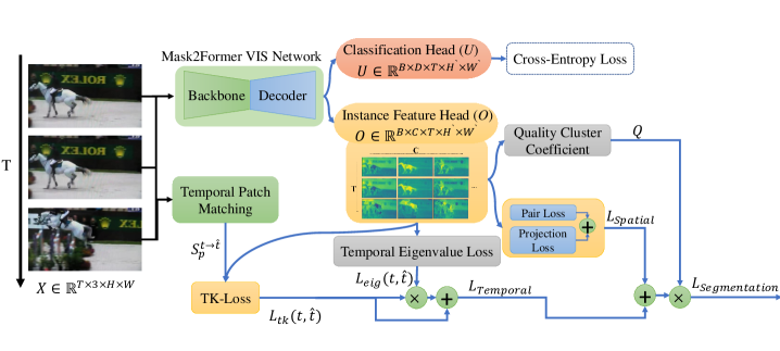
Figure 2: Pipelines of proposed Eigen-Cluster VIS. After inputting $X$ into Mask2former, two outputs, $U$ and $O$, are generated. According to Method [48], $X$ is also fed into the Temporal Patch Matching module to extract the corresponding patches for TK-Loss. $U$ pertains to classification and is optimized using Cross-Entropy Loss, while $O$ represents instance features from which the QCC, TEL, and TK-Loss modules are derived. All the losses are then aggregated under the title $L_{\text{segmentation}}$ during the training process, and the optimization is carried out.

III-A Overview

Figure 2 illustrates the overall pipeline of the proposed method. It is worth mentioning that the proposed method can be integrated with any backbone and supervised VIS model. In this research, the Mask2Former VIS is used with ResNet50-101 and Swin-L backbones. The input to the network is denoted as $X\in\mathbb{R}^{B\times T\times 3\times H\times W}$, where $B$ represents the number of three-channel color clips, $T$ is the number of frames, and $H$ and $W$ are the height and width of each frame, respectively.

To apply the Temporal KNN-patch Loss (TK-Loss), as described in [28], candidate patches must first be extracted from the input clip $X$. Then, the temporal matching is performed between these patches. If $p$ represents a patch location in frame $t$, the temporal matching yields the mapping $\mathcal{S}$, where $\mathcal{S}_{p}^{t\rightarrow\hat{t}}=\{\hat{p}_{i}\}_{i}$ provides the corresponding locations $\hat{p}$ in frame $\hat{t}$.

After obtaining the corresponding patches, the $X$ clip is fed into the Mask2Former network. The Mask2Former produces two outputs: $O\in\mathbb{R}^{B\times C\times T\times H^{\prime}\times W^{\prime}}$, which contains the features corresponding to the instances, and $U\in\mathbb{R}^{B\times D\times T\times H\times W}$, which is the classification matrix corresponding to $D$ categories. The classification matrix $U$ is optimized by using the cross-entropy function and the ground truth targets.

During the training phase, the losses and coefficients related to predicted instances in space and time are calculated from the output $O$. These calculations occur at different levels: i) at the spatio-temporal level, which includes the QCC; at the temporal level, which includes the TEL and TK_Loss; and ii) at the spatial level, which includes $L_{projection}$ and $L_{pair}$. The network weights are then optimized according to these criteria.

In the following sections, first the concept of spatio-temporal consistency is presented as it pertains to this research, followed by a detailed introduction of the proposed loss functions and coefficients for the VIS task.

III-B Spatio-Temporal Consistency

In the past, spatial compatibility modules often used a patch-oriented approach to address compatibility issues. A patch-oriented view, such as the TK-Loss approach, focuses on small areas like corresponding patches across frames. This can be achieved by working with predicted masks [73, 19] or using optical flow techniques as shown in [74, 75]. However, in addition to the patch-oriented view, a clip-oriented view examines compatibility over larger areas.

In this research, the QCC module is introduced to create a clip-oriented view. This module measures spatio-temporal coherence at the feature representation level of a video clip without requiring any knowledge of the ground truth mask regions. Although the patch-oriented view, like TK-Loss, strongly constrains the consistency of the mask for corresponding patches of instances across frames, it applies this constraint equally across all patches without accounting for inherent differences between frames.

In successive frames, instances may be deformed or occluded, or their appearance may change due to motion blur and brightness. Therefore, the degree of inter-frame changes in each clip varies and can be measured and applied in the loss function at the level of patches. With the TEL module, we aim to create a regularizing coefficient between frames based on the difference in eigenvalues. This coefficient controls the penalty amount in the loss at the level of corresponding patches. As shown in Figure 2, this controller increases the patch loss by multiplying the TK-Loss value that measures the loss at the patch level. Therefore, the more significant the difference in eigenvalues between frames, the greater the final temporal loss and, ultimately, the greater the effort to improve the accuracy of such frames. As demonstrated in Section 4, using eigenvalues as the controller coefficients effectively enhances the segmentation accuracy.

III-C Quality Cluster Coefficient

During the training process, specifically in the loss calculation stage, the output $O$ converges towards a suitable representation of each instance based on the ground truth mask. However, beyond just training with ground truth masks, it is possible to design a loss function that measures the discrimination of the features obtained without relying on the ground truth. This allows for an unsupervised evaluation of the output quality of $O$. Incorporating an unsupervised perspective enables the model to learn new aspects that might not be captured by the supervised view alone. This approach allows for better adaptation when the distribution of objects during testing differs significantly from that during training. By learning aspects independently of the ground truth and focusing more on the internal consistency of the output, the model can improve mask prediction accuracy and other related tasks.

To achieve this, a new metric called the QCC is introduced, which emphasizes the natural grouping consistency of features and promotes better segmentation of instances. The QCC as shown in Figure 3 is calculated by applying the K-means clustering (with K equal to the number of real instances) on $O$ and evaluating the quality of the resulting spatio-temporal clusters by using the Davies-Bouldin score [76]. By implementing this coefficient, the mismatch between the number of clusters and the type of clustering is reduced, allowing the model to converge towards denser clusters with a higher resolution gradually. This leads to better discrimination of the features representing the instances. The QCC measures the quality and discrimination of dense areas in space and time without considering the actual regions of the instances. This nearly unsupervised approach allows the network to self-evaluate its outputs, which can uncover new learning opportunities when combined with other loss functions that provide feedback from the real output. Note that this score is straightforward to implement and does not add any new parameters to the network. Further details on the main steps are explained in the follow:

1. Feature Transformation: Each instance feature $O\in\mathbb{R}^{B\times C\times T\times H^{\prime}\times W^{\prime}}$ is first resized using the scale factor $S$. Then, each batch is resized to the dimensions $F\in\mathbb{R}^{(TH^{\prime}W^{\prime}/S)\times C}$.

2. K-means Clustering: For each batch, the K-means algorithm is applied to cluster the transformed features into $K$ clusters. The K-means algorithm partitions $F$ into $K$ clusters $\{V_{1},V_{2},\ldots,V_{K}\}$ by minimizing the within-cluster variance. In this context, $f$ denotes an individual feature vector in $F$. The objective is defined as:

$$\min_{\{V_{k}\}}\sum_{k=1}^{K}\sum_{f\in V_{k}}\|f-\mu_{k}\|^{2}$$ (1)

where $\mu_{k}$ is the centroid of cluster $V_{k}$.

3. Davies-Bouldin Score: The quality of the clustering is evaluated using the Davies-Bouldin score, which is defined as:

$$d_{b}=\frac{1}{K}\sum_{i=1}^{K}\max_{j\neq i}\left(\frac{\sigma_{i}+\sigma_{j}}{dist(\mu_{i},\mu_{j})}\right),b\in B$$ (2)

where $\sigma_{i}$ is the average distance between each point in cluster $i$ and the centroid $\mu_{i}$. Also, $dist(\mu_{i},\mu_{j})$ is the Euclidean distance between centroids $\mu_{i}$ and $\mu_{j}$. Lower $d_{b}$ scores indicate better cluster quality.

4. Creating the Coefficient: Since QCC is considered a coefficient, the sum of the $d_{b}$ values plus one is chosen as the final value of $Q$:

$$Q=1+\frac{1}{B}\sum_{b\in B}d_{b},$$ (3)

which is then multiplied by the final loss. A lower value of $Q$ encourages the network to learn better features, leading to more distinct clusters.

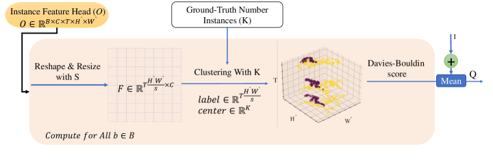
Figure 3: Quality Cluster Coefficient. Instance features are reshaped and resized along the spatial dimension for each clip in a batch. Subsequently, a K-means clustering (where K is the number of instances in the ground truth) is performed on these features. The Quality Cluster Coefficient is computed by using the Davies-Bouldin metric.

III-D Temporal Eigenvalue Loss

The goal of TEL, shown in Figure 4, is to ensure temporal consistency and coherence in VIS. As explained earlier, the eigenvalues derived from the Laplacian matrix of a graph adjacency matrix provide a robust representation of the structural and spatial properties in each graph. These eigenvalues offer essential information about the connectivity and smoothness of pixel links in each frame, making them useful in the graph segmentation process. For example, the second smallest eigenvalue, known as the algebraic connectivity or Fiedler value, reflects the algebraic connectivity and is related to the sparsest cut and spectral gap. Other eigenvalues can represent the structure of the graph at higher levels of abstraction.

By converting the output $O$ to an adjacency matrix, the characteristics of eigenvalues can be utilized in the context of input video frames. Ensuring that eigenvalues are close to each other between successive frames is crucial for maintaining temporal coherence. Time warping in segmentation tasks helps to avoid flickering and non-contiguous segmentation in frames, which are common problems in video analysis. Minimizing the MAE between eigenvalues of adjacent frames promotes smoother transitions and more stable segmentation boundaries over time.

This alignment of eigenvalues across frames reduces temporal discontinuities and increases the overall quality and reliability of the segmentation output, resulting in more consistent and visually pleasing results. One of the important features of this loss function is the small dimensions of the compared data, making the optimization process easier and not imposing an additional burden on the overall network optimization process. Note that this loss function does not add any parameters to the network. The main steps of this loss function are outlined below.

1. Select the Corresponding Pair: For each real instance $i\in\{1,\ldots,I\}$ in batch $b\in\{1,\ldots,B\}$, we determine the corresponding channel $c_{i}$ from the prediction matrix $O$ by using the Hungarian algorithm [77]. This result is a set of pairs $R=\{(i,c_{i})\}_{i=1}^{I}$, where $c_{i}$ is the selected channel for instance $i$. The total number of pairs $(i,c_{i})$ across all batches is $N=B\times I$. Using these pairs $R$, a target matrix $E\in\mathbb{R}^{N\times T\times H^{\prime}\times W^{\prime}}$ is constructed. The elements of $E$ are obtained by indexing $O$ with the selected channels from $R$.

2. Feature Transformation and Affinity Matrix Construction: For each $t\in T$ and each $n\in N$, we first resize the $E$ matrix by a scale factor $S$ and then reshape it as follows:

$$E_{(n,t)}\in\mathbb{R}^{\frac{H^{\prime}W^{\prime}}{S}\times 1}.$$ (4)

Next, the affinity matrix $A_{(n,t)}\in\mathbb{R}^{\frac{H^{\prime}W^{\prime}}{S}\times\frac{H^{\prime}W^{\prime}}{S}}$ is constructed by:

$$A_{(n,t)}=E_{(n,t)}E_{(n,t)}^{T}\odot\left(E_{(n,t)}E_{(n,t)}^{T}>0\right)$$ (5)

where $\odot$ denotes the element-wise multiplication. The affinities are thresholded at $0$ because the features are intended for aggregating similar features rather than anti-correlated features.

3. Building the Laplacian Matrix and Decomposing it into Eigenvalues: First, the Degree Matrix $D_{(n,t)}$ is calculated as:

$$D_{(n,t)}=\sum_{j}A_{(n,t)}(i,j).$$ (6)

Then, the Laplacian matrix is constructed as: $La_{(n,t)}$:

$$La_{(n,t)}=D_{(n,t)}-A_{(n,t)}.$$ (7)

Finally, $La_{(n,t)}$ is decomposed to obtain the first $Y$ eigenvalues, resulting in:

$$\{\lambda_{1},\lambda_{2},\ldots,\lambda_{Y}\}=\text{Eig}(La_{(n,t)},Y)\in\mathbb{R}^{Y}.$$ (8)

4. Calculation of Loss: All eigenvalues are stacked at the level of each $n\in N$ to get $\Lambda_{t}$:

$$\Lambda_{t}=\text{Stack}([\lambda_{1},\lambda_{2},\ldots,\lambda_{Y}])\in\mathbb{R}^{N\times Y}.$$ (9)

Then, the eigenvalue loss $\mathcal{L}_{\text{eig}}(\hat{t},t)$ is calculated using the following relationship:

$$\mathcal{L}_{\text{eig}}(t,\hat{t})=\|\Lambda_{\hat{t}}-\Lambda_{t}\|_{1}.$$ (10)

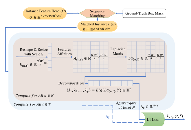
Figure 4: Temporal Eigenvalue Loss. Matched instances are identified through sequence matching between the instance features and ground truth masks. Subsequently, for each instance in every frame, the features are resized and reshaped, followed by the creation of an affinity matrix based on these features. Eigenvalues of the Laplacian of this affinity matrix are extracted for each instance. The MAE loss is then computed cyclically between the corresponding instances in every two consecutive frames.

III-E Segmentation Loss

As explained in [48], the TK-loss, denoted as $L_{\text{tk}}(t,\hat{t})$, is derived by considering the matrix $O$, the locations $p$, and the mapping $\mathcal{S}_{p}^{t\rightarrow\hat{t}}$. This can be expressed more simply as:

$$\tau=M^{t}_{p}M^{\hat{t}}_{\hat{p}}+(1-M^{t}_{p})(1-M^{\hat{t}}_{\hat{p}}),$$ (11)

$$L_{\text{tk}}(t,\hat{t})=\frac{1}{H^{\prime}W^{\prime}}\sum_{p}\sum_{\hat{p}\in\mathcal{S}^{t\rightarrow\hat{t}}}-\log(\tau),$$ (12)

where $M^{t}_{p}\in[0,1]$ represents the predicted binary instance mask of an object, evaluated at position $p$ in frame $t$.

According to the given explanations, $L_{\text{eig}}(t,\hat{t})$ is first multiplied by $L_{\text{tk}}(t,\hat{t})$, and then added again with $L_{\text{tk}}(t,\hat{t})$ to finally obtain the temporal loss $L_{\text{temporal}}$, as:

$$\psi(t,\hat{t})=L_{\text{tk}}(t,\hat{t})+\beta\left(L_{\text{tk}}(t,\hat{t})\times L_{\text{eig}}(t,\hat{t})\right),$$ (13)

$$L_{\text{temporal}}=\sum_{t=1}^{T}\begin{cases}\psi(t,t+1)&\text{if }t<T-1\\ \psi(t+1,0)&\text{if }t=T-1\end{cases},$$ (14)

where $\beta$ is a hyperparameter chosen according to the complexity of the backbone.

Since the proposed method is based on weak supervision and does not involve ground truth masks, we draw inspiration from [24] to estimate a spatial loss, $L_{\text{spatial}}$, using two components: the Box Projection Loss $L_{\text{proj}}$ and the Pairwise Loss $L_{\text{pair}}$. The Box Projection Loss $L_{\text{proj}}$ measures the compatibility between the predicted and ground truth bounding boxes by projecting the predicted and ground truth masks along the $x$ and $y$ axes, using the Dice loss function. The concept behind $L_{\text{pair}}$ is that pixels with similar colors most probably belong to the same predicted mask.

After obtaining the spatial loss and temporal loss and multiplying them by $Q$, which indicates the clustering quality in space-time, the final segmentation loss $L_{\text{seg}}$ can be computed as:

$$L_{\text{segmentation}}=Q^{\alpha}\times\left(L_{\text{spatial}}+L_{\text{temporal}}\right)$$

where $\alpha$ is a value of zero or one used in the training process, as described in Section 4.

As described in [28], during the instance-sequence matching step, the predicted and ground truth masks are first converted into box masks. Then, random points are sampled from these masks using the Dice IoU loss function to identify the best pairs of predicted and ground truth masks.

IV EXPERIMENTS

This section begins by introducing the experimental datasets and evaluation metrics. It then explains the implementation methods. Finally, the experiments and ablation studies are presented and discussed.

TABLE I: Comparison on the YouTube-VIS 2019 validation dataset: I refers to the use of the COCO dataset during pre-training at the image mask level, while V indicates that video masks were used during the training process.

Method	Mask ann.	Backbone	AP	$AP_{50}$	$AP_{75}$	$AR_{1}$	$AR_{10}$
Fully-supervised:
PCAN [78]	I+V	Res50	36.1	54.9	39.4	36.3	41.6
EfficientVIS [79]	I+V	Res50	37.9	59.7	43.0	40.3	46.6
InsPro [80]	I+V	Res50	40.0	62.9	43.1	37.6	44.5
IFC [45]	I+V	Res50	42.8	65.8	46.8	43.8	51.2
SeqFormer [8]	I+V	Res50	47.4	69.8	51.8	45.5	54.8
Mask2Former [9]	I+V	Res50	47.8	69.2	52.7	46.2	56.6
VMT [81]	I+V	Res50	47.9	-	52.0	45.8	-
GenVIS [36]	I+V	Res50	50.0	71.5	54.6	49.5	59.7
DVIS [51]	I+V	Res50	51.2	73.8	57.1	47.2	59.3
Weakly-supervised:
FlowIRN [19]	-	Res50	10.5	27.2	6.2	12.3	13.6
SOLO-Track [54]	I	Res50	30.6	50.7	33.5	31.6	37.1
Cluster2Former [14]	I	Res50	38.3	62.5	42.5	39.3	46.6
Mask2Former + BoxInst [24]	-	Res50	38.6	64.2	38.5	38.0	46.8
Mask2Former + Mask-free VIS [28]	I	Res50	46.6	72.5	49.7	44.9	55.7
Mask2Former + Eigen-Cluster VIS	I	Res50	47.4	72.7	50.1	45.7	57.2
Fully-supervised:
PCAN [78]	I+V	Res101	37.6	57.2	41.3	37.2	43.9
EfficientVIS [79]	I+V	Res101	39.8	61.8	44.7	42.1	49.8
IFC [45]	I+V	Res101	44.6	69.2	49.5	44.0	52.1
SeqFormer [8]	I+V	Res101	49.0	71.1	55.7	46.8	56.9
VMAT [81]	I+V	Res101	49.4	-	56.4	46.7	-
Mask2Former [9]	I+V	Res101	49.8	73.6	55.4	48.0	58.0
Weakly-supervised:
Mask2Former + BoxInst [24]	-	Res101	40.8	67.8	42.2	40.0	49.2
Mask2Former + Mask-free VIS [28]	I	Res101	48.9	74.9	54.7	44.9	57.0
Mask2Former + Eigen-Cluster VIS	I	Res101	49.7	75.8	54.6	46.6	58.5
Fully-supervised:
SeqFormer [8]	I+V	SwinL	59.3	82.1	66.4	51.7	64.4
VMAT [81]	I+V	SwinL	59.7	-	66.7	52.0	-
Mask2Former [9]	I+V	SwinL	60.4	84.4	67.0	-	-
DVIS [51]	I+V	SwinL	63.9	78.2	70.4	56.2	69.0
GenVIS [36]	I+V	SwinL	64.0	84.9	68.3	56.1	69.4
Weakly-supervised:
Mask2Former + BoxInst [24]	-	SwinL	49.8	73.2	55.5	48.2	58.1
Mask2Former + Mask-free VIS [28]	I	SwinL	55.3	82.5	60.8	50.7	62.2
Mask2Former + Eigen-Cluster VIS	I	SwinL	56.8	83.7	62.9	51.7	63.1

IV-A Dataset and Evaluation Metrics

IV-A1 Datasets

Two datasets, YouTube-VIS 2019/2021 [5] and OVIS [6], were used for experiments in the VIS task. YouTube-VIS 2019 contains 2,238 videos across 40 categories, mainly featuring animals, humans, and sports activities. In the 2021 version, the dataset has expanded to 3,032 videos, with some class categories differing from the previous version. OVIS, a VIS dataset with 607 videos across 25 categories, focuses on animals and humans. It presents more challenging conditions than the YouTube-VIS datasets due to a higher number of instances per video and greater occlusion, measured by MBOR [6]. The instance-to-video ratio is 1.69 for YouTube-VIS 2019, 2.10 for YouTube-VIS 2021, and 5.80 for OVIS. The MBOR values are 0.07 and 0.06 for YouTube-VIS 2019 and 2021, respectively, and 0.22 for OVIS.

IV-A2 Evaluation Metrics

Following the COCO [27] guidelines and methodology of [5], the evaluation metrics are based on AP, AP50, AP75, AR1, and AR10.

IV-B Implementation Details

As mentioned earlier, the Mask2Former network is used as the baseline for the VIS task in this research. All settings of this network are preserved, except for the loss function and sequence matching components. The loss function follows the TK-Loss settings as outlined in [28]. The training process is divided into three stages. The first stage involves pre-training with the COCO dataset using image-level masks. In contrast, the second and third stages involve the main training process, where no ground-truth masks are available, and only bounding box information is used.

In the first and second stages, all backbone and network head weights are optimized with $\alpha=0$ and $\beta=0$ settings. In the third stage, the backbone is frozen, and $\beta$ is adjusted based on backbone complexity settings, with $\alpha$ set to 1. The batch size is 16 in the first and second stages and 2 in the third stage. The number of iterations is 60k for the first stage, 6k for the second stage, and up to 4k for the third stage, depending on different backbones. The AdamW optimization technique is used with a learning rate of $10^{-4}$ in all three stages. In the QCC and TEL modules, we set $S=4$ to reduce dimensions, and the number of extracted eigenvalues was $Y=3$.

IV-C Comparison with State-of-the-art Methods

The proposed Eigen-cluster VIS is compared to state-of-the-art methods in weak and fully supervised settings. Table I presents the evaluation results on the YouTube-VIS 2019 validation set across three backbones: R50, R101, and SwinL.

For the R50 backbone, Eigen-cluster VIS achieves an AP of 47.4, demonstrating clear superiority over fully supervised methods such as EfficientVIS[79], PCAN[78], INSpro [80], IFC [45], and matching the AP of SeqFormer[8]. Additionally, in this backbone shows an improvement of 0.8% over the Mask-freeVIS method and reduces the performance gap between Weakly-supervised methods and Mask2Former[9] from 1.2 to 0.4.

With the R101 backbone, our proposed method achieves an AP of 49.7, outperforming fully supervised methods[79],[45] and [8]. It also improves by 0.8% over the MaskFreeVIS method, narrowing the gap between Weakly-supervised methods and Mask2Former from 0.9 to 0.1.

In the SwinL backbone, which employs a transformer architecture, fully supervised methods generally exhibit higher accuracy than other backbones. However, our proposed method reduces the performance gap between Weakly-supervised methods and Mask2Former from 5.1 to 3.6, achieving an AP of 56.8.

IV-D Ablation study

The method presented in [48] provides a valuable comparison of various temporal matching schemes designed to enhance the performance of temporal matching algorithms in the VIS task, as shown in Table II. These temporal matching schemes can be integrated into the loss function to ensure consistency between instance masks over time. As shown in Table II, the proposed temporal matching achieved an AP of 44.0, improving the previous best matching method by 1.5

A significant advantage of the matching algorithm presented in this research is that it introduces no additional learnable parameters. Furthermore, its clip-oriented design enables improved performance in occluded areas. In contrast, flow-based [20] algorithms struggle when an object’s pixels are occluded in other frames, leading to inaccurate predictions of pixel flow and consistency in those areas. Other matching algorithms, such as Deformable[19] Matching and the set of Learnable Pixel/Patch Matching, 3D Pairwise Matching, and Temporal KNN-Matching introduced by [48], provide only a patch-oriented perspective. In contrast, our proposed method also incorporates a clip-oriented view, resulting in higher accuracy than other methods.

The effect of different modules, both individually and in combination, is shown in Table III. Adding the TEL module increases AP by 1.1%. When both AP modules are added, the accuracy reaches 44.0, demonstrating the effectiveness of these modules. Figure 5 illustrates the impact of adding and removing the proposed modules.

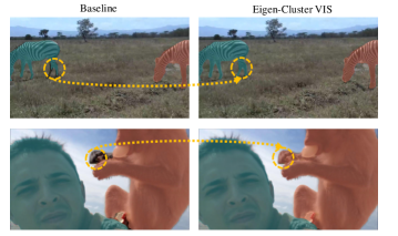
Figure 5: Visualization of Baseline and Eigen-Cluster VIS Differences. In the baseline, some foreground areas may be missed, particularly in details involving fast movements. These missed regions are indicated with dashed lines.

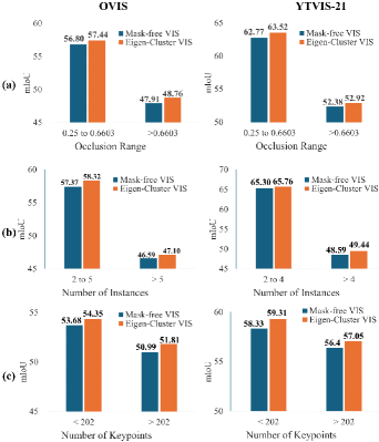
Figure 6: mIoU evaluation across the YouTube-VIS 2021 (YTVIS-21) and OVIS datasets, examining three characteristics. (a) mIoU concerning occlusion, (b) mIoU in relation to the number of instances, and (c) mIoU based on the number of keypoints.

In addition, Table IV shows the impact of $Y$ on segmentation accuracy. As evident, the best performance was achieved when ${Y=3}$.

TABLE II: Comparison of Temporal Matching Schemes on Youtube-VIS 2019 validation set. The term ”Param” refers to whether a learnable parameter is added to the model.

Temporal Matching Scheme	Param	AP	AP50	AP75	AR1	AR10
Baseline (No Matching)	✗	38.6	65.9	38.8	38.4	47.7
3D Pairwise Matching	✗	39.4	65.0	41.7	40.2	48.0
Learnable Pixel Matching	✓	39.5	65.7	40.2	39.7	48.4
Temporal Deformable Matching	✓	39.6	65.9	40.1	39.9	48.6
Flow-based Matching	✓	40.2	66.3	41.9	40.5	49.1
Learnable Patch Matching	✓	40.6	66.5	42.6	40.3	49.2
Temporal KNN-Matching (TK)	✗	42.5	66.8	45.7	41.2	51.2
Temporal EigenValue + TK	✗	44.0	68.9	48.0	41.9	52.0

TABLE III: An ablation study to analyze the impact of proposed components on Youtube-VIS 2019 validation set.

TEL	QCC	AP	AP50	AP75	AR1	AR10
		42.5	66.8	45.7	41.2	51.2
✓		43.6	68.5	46.9	41.5	51.6
✓	✓	44.0	68.9	48.0	41.9	52.0

TABLE IV: Impact of the number of eigenvalues Y on segmentation accuracy on Youtube-VIS 2019 validation set.

Y	AP	AP50	AP75	AR1	AR10
2	43.8	68.4	47.8	41.9	51.8
3	44.0	68.9	48.0	41.9	52.0
4	43.6	68.2	46.9	41.8	51.5

Previous research has not reported the effect of the inherent characteristics of videos on the obtained accuracy, primarily because ground-truth validation tags have not been publicly released. As a result, it has been difficult to measure the accuracy of different methods based on various factors, such as occlusions, the number of instances, and the number of image keypoints. To address this, we conducted an experiment to evaluate the accuracy of a model trained on YouTube-VIS2019 across different video attributes. The model was tested without exposure to the YouTube-VIS2021 and OVIS datasets during training. Since the classes used for training and testing are different, we only utilized the mIoU metric. Table V presents the experimental results of the model trained on YouTube-VIS2019 and tested on YouTube-VIS2021 and OVIS datasets using the SwinL backbone. Due to the overlap of some videos between YouTube-VIS2021 and YouTube-VIS2019, we tested only 794 new videos that were not present in the older version. In Table V, the selected videos had a maximum ${T=36}$ and MBOR${\geq 2}$ . As shown in the table, Eigen-cluster VIS improved the mIoU by 0.63% compared to MaskFreeVIS on the YouTube-VIS2021 dataset. On the OVIS dataset, the mIoU improvement reached 0.74%, demonstrating the greater generalizability of the method.

TABLE V: mIoU in Youtube-VIS 2021 and OVIS datasets.

model	Youtube-VIS 2021	OVIS
MaskfreeVIS	57.53	52.34
Eigen-Cluster VIS	58.16	53.08

From Table V, the graphs in Figure 6 can be derived. In this chart, mIoU is reported based on three characteristics: occlusion, the number of instances, and the number of keypoints. Occlusion is measured using the MBOR criterion, and keypoints are extracted using the SIFT algorithm [82]. Due to the unique characteristics of each dataset, we calculate the median value for each dataset and characteristic and then assess the accuracy on either side of these median values.

Part (a) of Figure 6 shows the relationship between MBOR values and segmentation performance. Generally, higher MBOR values lead to lower segmentation performance. Our proposed method improves accuracy by 0.54% over MaskFreeVIS in the higher MBOR interval of the YouTube-VIS 2021 dataset, and by 0.85% in the OVIS dataset.

Part (b) of Figure 6 demonstrates how segmentation performance decreases as the number of instances increases. Our method outperforms MaskFreeVIS by 0.85% in the higher instance interval of the YouTube-VIS 2021 dataset and by 0.51% in the OVIS dataset.

Part (c) of Figure 6 highlights the effect of the number of video foreground keypoints on segmentation accuracy. Fewer keypoints generally result in better detection due to smoother textures in the foreground. Our method shows a 0.65% improvement over MaskFreeVIS in the higher keypoint interval of the YouTube-VIS 2021 dataset, and a 0.82% improvement in the OVIS dataset.

V Conclusion

In this paper, the Eigen-Cluster VIS model, which is a weakly supervised approach to video instance segmentation, was proposed. This method effectively narrowed the gap between the weakly supervised and fully supervised techniques without requiring ground truth masks at the video level. By introducing the Quality Cluster Coefficient module, a criterion for discriminating spatio-temporal instances without the need for ground truth regions was established. Additionally, the Temporal Eigenvalue Loss was introduced, which leverages the eigenvalue information of frames to create smoother transitions and enhance mask consistency across frames within a video clip. This simultaneous focus on both spatial and temporal dimensions, from the image patch level to the clip level, resulted in a VIS model that demonstrated strong performance compared to previous methods. Eigen-cluster VIS offers potential for further development in both representation and optimization processes and can be integrated with fully unsupervised methods, which we plan to explore in our future work.

References

- [1] P. Voigtlaender, M. Krause, A. Osep, J. Luiten, B. B. G. Sekar, A. Geiger, and B. Leibe, “Mots: Multi-object tracking and segmentation,” in Proceedings of the ieee/cvf conference on computer vision and pattern recognition, 2019, pp. 7942–7951.
- [2] M. Elhoseny, “Multi-object detection and tracking (modt) machine learning model for real-time video surveillance systems,” Circuits, Systems, and Signal Processing, vol. 39, no. 2, pp. 611–630, 2020.
- [3] A. M. Mansourian, V. Somers, C. De Vleeschouwer, and S. Kasaei, “Multi-task learning for joint re-identification, team affiliation, and role classification for sports visual tracking,” in Proceedings of the 6th International Workshop on Multimedia Content Analysis in Sports, 2023, pp. 103–112.
- [4] V. Somers, V. Joos, A. Cioppa, S. Giancola, S. A. Ghasemzadeh, F. Magera, B. Standaert, A. M. Mansourian, X. Zhou, S. Kasaei et al., “Soccernet game state reconstruction: End-to-end athlete tracking and identification on a minimap,” in Proceedings of the IEEE/CVF Conference on Computer Vision and Pattern Recognition, 2024, pp. 3293–3305.
- [5] L. Yang, Y. Fan, and N. Xu, “Video instance segmentation,” in Proceedings of the IEEE/CVF international conference on computer vision, 2019, pp. 5188–5197.
- [6] J. Qi, Y. Gao, Y. Hu, X. Wang, X. Liu, X. Bai, S. Belongie, A. Yuille, P. H. Torr, and S. Bai, “Occluded video instance segmentation: A benchmark,” International Journal of Computer Vision, vol. 130, no. 8, pp. 2022–2039, 2022.
- [7] Y. Wang, Z. Xu, X. Wang, C. Shen, B. Cheng, H. Shen, and H. Xia, “End-to-end video instance segmentation with transformers,” in Proceedings of the IEEE/CVF conference on computer vision and pattern recognition, 2021, pp. 8741–8750.
- [8] J. Wu, Y. Jiang, S. Bai, W. Zhang, and X. Bai, “Seqformer: Sequential transformer for video instance segmentation,” in European Conference on Computer Vision. Springer, 2022, pp. 553–569.
- [9] B. Cheng, A. Choudhuri, I. Misra, A. Kirillov, R. Girdhar, and A. G. Schwing, “Mask2former for video instance segmentation,” arXiv preprint arXiv:2112.10764, 2021.
- [10] A. Khoreva, R. Benenson, J. Hosang, M. Hein, and B. Schiele, “Simple does it: Weakly supervised instance and semantic segmentation,” in Proceedings of the IEEE conference on computer vision and pattern recognition, 2017, pp. 876–885.
- [11] J. Lee, J. Yi, C. Shin, and S. Yoon, “Bbam: Bounding box attribution map for weakly supervised semantic and instance segmentation,” in Proceedings of the IEEE/CVF conference on computer vision and pattern recognition, 2021, pp. 2643–2652.
- [12] B. Cheng, O. Parkhi, and A. Kirillov, “Pointly-supervised instance segmentation,” in Proceedings of the IEEE/CVF Conference on Computer Vision and Pattern Recognition, 2022, pp. 2617–2626.
- [13] H. Lee, S. Hwang, and S. Kwak, “Extreme point supervised instance segmentation,” in Proceedings of the IEEE/CVF Conference on Computer Vision and Pattern Recognition, 2024, pp. 17 212–17 222.
- [14] Á. Fóthi, A. Szlatincsán, and E. Somfai, “Cluster2former: Semisupervised clustering transformers for video instance segmentation,” Sensors, vol. 24, no. 3, p. 997, 2024.
- [15] X. Wang, R. Girdhar, S. X. Yu, and I. Misra, “Cut and learn for unsupervised object detection and instance segmentation,” in Proceedings of the IEEE/CVF conference on computer vision and pattern recognition, 2023, pp. 3124–3134.
- [16] X. Wang, I. Misra, Z. Zeng, R. Girdhar, and T. Darrell, “Videocutler: Surprisingly simple unsupervised video instance segmentation,” in Proceedings of the IEEE/CVF Conference on Computer Vision and Pattern Recognition, 2024, pp. 22 755–22 764.
- [17] S. Huang, S. Suri, K. Gupta, S. S. Rambhatla, S.-n. Lim, and A. Shrivastava, “Uvis: Unsupervised video instance segmentation,” in Proceedings of the IEEE/CVF Conference on Computer Vision and Pattern Recognition, 2024, pp. 2682–2692.
- [18] J. Ahn, S. Cho, and S. Kwak, “Weakly supervised learning of instance segmentation with inter-pixel relations,” in Proceedings of the IEEE/CVF conference on computer vision and pattern recognition, 2019, pp. 2209–2218.
- [19] Q. Liu, V. Ramanathan, D. Mahajan, A. Yuille, and Z. Yang, “Weakly supervised instance segmentation for videos with temporal mask consistency,” in Proceedings of the IEEE/CVF Conference on Computer Vision and Pattern Recognition, 2021, pp. 13 968–13 978.
- [20] Z. Teed and J. Deng, “Raft: Recurrent all-pairs field transforms for optical flow,” in Computer Vision–ECCV 2020: 16th European Conference, Glasgow, UK, August 23–28, 2020, Proceedings, Part II 16. Springer, 2020, pp. 402–419.
- [21] N. Eslami, F. Arefi, A. M. Mansourian, and S. Kasaei, “Rethinking raft for efficient optical flow,” in 2024 13th Iranian/3rd International Machine Vision and Image Processing Conference (MVIP). IEEE, 2024, pp. 1–7.
- [22] C.-C. Hsu, K.-J. Hsu, C.-C. Tsai, Y.-Y. Lin, and Y.-Y. Chuang, “Weakly supervised instance segmentation using the bounding box tightness prior,” Advances in neural information processing systems, vol. 32, 2019.
- [23] S. Lan, Z. Yu, C. Choy, S. Radhakrishnan, G. Liu, Y. Zhu, L. S. Davis, and A. Anandkumar, “Discobox: Weakly supervised instance segmentation and semantic correspondence from box supervision,” in Proceedings of the IEEE/CVF International Conference on Computer Vision, 2021, pp. 3406–3416.
- [24] Z. Tian, C. Shen, X. Wang, and H. Chen, “Boxinst: High-performance instance segmentation with box annotations,” in Proceedings of the IEEE/CVF Conference on Computer Vision and Pattern Recognition, 2021, pp. 5443–5452.
- [25] W. Li, W. Liu, J. Zhu, M. Cui, X.-S. Hua, and L. Zhang, “Box-supervised instance segmentation with level set evolution,” in European conference on computer vision. Springer, 2022, pp. 1–18.
- [26] R. Li, C. He, Y. Zhang, S. Li, L. Chen, and L. Zhang, “Sim: Semantic-aware instance mask generation for box-supervised instance segmentation,” in Proceedings of the IEEE/CVF Conference on Computer Vision and Pattern Recognition, 2023, pp. 7193–7203.
- [27] T.-Y. Lin, M. Maire, S. Belongie, J. Hays, P. Perona, D. Ramanan, P. Dollár, and C. L. Zitnick, “Microsoft coco: Common objects in context,” in Computer Vision–ECCV 2014: 13th European Conference, Zurich, Switzerland, September 6-12, 2014, Proceedings, Part V 13. Springer, 2014, pp. 740–755.
- [28] L. Ke, M. Danelljan, H. Ding, Y.-W. Tai, C.-K. Tang, and F. Yu, “Mask-free video instance segmentation,” in Proceedings of the IEEE/CVF Conference on Computer Vision and Pattern Recognition, 2023, pp. 22 857–22 866.
- [29] L. Melas-Kyriazi, C. Rupprecht, I. Laina, and A. Vedaldi, “Deep spectral methods: A surprisingly strong baseline for unsupervised semantic segmentation and localization,” in Proceedings of the IEEE/CVF Conference on Computer Vision and Pattern Recognition, 2022, pp. 8364–8375.
- [30] G. Bertasius and L. Torresani, “Classifying, segmenting, and tracking object instances in video with mask propagation,” in Proceedings of the IEEE/CVF Conference on Computer Vision and Pattern Recognition, 2020, pp. 9739–9748.
- [31] H. Lin, R. Wu, S. Liu, J. Lu, and J. Jia, “Video instance segmentation with a propose-reduce paradigm,” in Proceedings of the IEEE/CVF International Conference on Computer Vision, 2021, pp. 1739–1748.
- [32] S. Yang, Y. Fang, X. Wang, Y. Li, C. Fang, Y. Shan, B. Feng, and W. Liu, “Crossover learning for fast online video instance segmentation,” in proceedings of the IEEE/CVF international conference on computer vision, 2021, pp. 8043–8052.
- [33] X. Li, H. He, Y. Yang, H. Ding, K. Yang, G. Cheng, Y. Tong, and D. Tao, “Improving video instance segmentation via temporal pyramid routing,” IEEE Transactions on Pattern Analysis and Machine Intelligence, vol. 45, no. 5, pp. 6594–6601, 2022.
- [34] J. Li, B. Yu, Y. Rao, J. Zhou, and J. Lu, “Tcovis: Temporally consistent online video instance segmentation,” in Proceedings of the IEEE/CVF International Conference on Computer Vision, 2023, pp. 1097–1107.
- [35] K. Ying, Q. Zhong, W. Mao, Z. Wang, H. Chen, L. Y. Wu, Y. Liu, C. Fan, Y. Zhuge, and C. Shen, “Ctvis: Consistent training for online video instance segmentation,” in Proceedings of the IEEE/CVF International Conference on Computer Vision, 2023, pp. 899–908.
- [36] M. Heo, S. Hwang, J. Hyun, H. Kim, S. W. Oh, J.-Y. Lee, and S. J. Kim, “A generalized framework for video instance segmentation,” in Proceedings of the IEEE/CVF Conference on Computer Vision and Pattern Recognition, 2023, pp. 14 623–14 632.
- [37] K. He, G. Gkioxari, P. Dollár, and R. Girshick, “Mask r-cnn,” in Proceedings of the IEEE international conference on computer vision, 2017, pp. 2961–2969.
- [38] L. Ke, Y.-W. Tai, and C.-K. Tang, “Deep occlusion-aware instance segmentation with overlapping bilayers,” in Proceedings of the IEEE/CVF conference on computer vision and pattern recognition, 2021, pp. 4019–4028.
- [39] J. Cao, R. M. Anwer, H. Cholakkal, F. S. Khan, Y. Pang, and L. Shao, “Sipmask: Spatial information preservation for fast image and video instance segmentation,” in Computer Vision–ECCV 2020: 16th European Conference, Glasgow, UK, August 23–28, 2020, Proceedings, Part XIV 16. Springer, 2020, pp. 1–18.
- [40] D. Liu, Y. Cui, W. Tan, and Y. Chen, “Sg-net: Spatial granularity network for one-stage video instance segmentation,” in Proceedings of the IEEE/CVF conference on computer vision and pattern recognition, 2021, pp. 9816–9825.
- [41] M. Li, S. Li, L. Li, and L. Zhang, “Spatial feature calibration and temporal fusion for effective one-stage video instance segmentation,” in Proceedings of the IEEE/CVF Conference on Computer Vision and Pattern Recognition, 2021, pp. 11 215–11 224.
- [42] X. Li, H. Yuan, W. Zhang, G. Cheng, J. Pang, and C. C. Loy, “Tube-link: A flexible cross tube framework for universal video segmentation,” in Proceedings of the IEEE/CVF International Conference on Computer Vision, 2023, pp. 13 923–13 933.
- [43] X. Li, J. Wang, X. Li, and Y. Lu, “Video instance segmentation by instance flow assembly,” IEEE Transactions on Multimedia, vol. 25, pp. 7469–7479, 2022.
- [44] A. Athar, S. Mahadevan, A. Osep, L. Leal-Taixé, and B. Leibe, “Stem-seg: Spatio-temporal embeddings for instance segmentation in videos,” in Computer Vision–ECCV 2020: 16th European Conference, Glasgow, UK, August 23–28, 2020, Proceedings, Part XI 16. Springer, 2020, pp. 158–177.
- [45] S. Hwang, M. Heo, S. W. Oh, and S. J. Kim, “Video instance segmentation using inter-frame communication transformers,” Advances in Neural Information Processing Systems, vol. 34, pp. 13 352–13 363, 2021.
- [46] O. Thawakar, S. Narayan, J. Cao, H. Cholakkal, R. M. Anwer, M. H. Khan, S. Khan, M. Felsberg, and F. S. Khan, “Video instance segmentation via multi-scale spatio-temporal split attention transformer,” in European Conference on Computer Vision. Springer, 2022, pp. 666–681.
- [47] S. Yang, X. Wang, Y. Li, Y. Fang, J. Fang, W. Liu, X. Zhao, and Y. Shan, “Temporally efficient vision transformer for video instance segmentation,” in Proceedings of the IEEE/CVF conference on computer vision and pattern recognition, 2022, pp. 2885–2895.
- [48] L. Ke, M. Danelljan, X. Li, Y.-W. Tai, C.-K. Tang, and F. Yu, “Mask transfiner for high-quality instance segmentation,” in Proceedings of the IEEE/CVF Conference on Computer Vision and Pattern Recognition, 2022, pp. 4412–4421.
- [49] J. Wu, Q. Liu, Y. Jiang, S. Bai, A. Yuille, and X. Bai, “In defense of online models for video instance segmentation,” in European Conference on Computer Vision. Springer, 2022, pp. 588–605.
- [50] M. Heo, S. Hwang, S. W. Oh, J.-Y. Lee, and S. J. Kim, “Vita: Video instance segmentation via object token association,” Advances in Neural Information Processing Systems, vol. 35, pp. 23 109–23 120, 2022.
- [51] T. Zhang, X. Tian, Y. Wu, S. Ji, X. Wang, Y. Zhang, and P. Wan, “Dvis: Decoupled video instance segmentation framework,” in Proceedings of the IEEE/CVF International Conference on Computer Vision, 2023, pp. 1282–1291.
- [52] J. Dai, K. He, and J. Sun, “Boxsup: Exploiting bounding boxes to supervise convolutional networks for semantic segmentation,” in Proceedings of the IEEE international conference on computer vision, 2015, pp. 1635–1643.
- [53] T. Cheng, X. Wang, S. Chen, Q. Zhang, and W. Liu, “Boxteacher: Exploring high-quality pseudo labels for weakly supervised instance segmentation,” in Proceedings of the IEEE/CVF Conference on Computer Vision and Pattern Recognition, 2023, pp. 3145–3154.
- [54] Y. Fu, S. Liu, U. Iqbal, S. De Mello, H. Shi, and J. Kautz, “Learning to track instances without video annotations,” in Proceedings of the IEEE/CVF Conference on Computer Vision and Pattern Recognition, 2021, pp. 8680–8689.
- [55] D.-A. Huang, Z. Yu, and A. Anandkumar, “Minvis: A minimal video instance segmentation framework without video-based training,” Advances in Neural Information Processing Systems, vol. 35, pp. 31 265–31 277, 2022.
- [56] M. Caron, H. Touvron, I. Misra, H. Jégou, J. Mairal, P. Bojanowski, and A. Joulin, “Emerging properties in self-supervised vision transformers,” in Proceedings of the IEEE/CVF international conference on computer vision, 2021, pp. 9650–9660.
- [57] A. Radford, J. W. Kim, C. Hallacy, A. Ramesh, G. Goh, S. Agarwal, G. Sastry, A. Askell, P. Mishkin, J. Clark et al., “Learning transferable visual models from natural language supervision,” in International conference on machine learning. PMLR, 2021, pp. 8748–8763.
- [58] Z. Yang, D. Liu, W. Cheng, J. Wang, and Y. Wu, “Pm-vis: High-performance box-supervised video instance segmentation,” arXiv preprint arXiv:2404.13863, 2024.
- [59] J. Cheeger, “A lower bound for the smallest eigenvalue of the laplacian,” Problems in analysis, vol. 625, no. 195-199, p. 110, 1970.
- [60] W. E. Donath and A. J. Hoffman, “Lower bounds for the partitioning of graphs,” IBM Journal of Research and Development, vol. 17, no. 5, pp. 420–425, 1973.
- [61] M. Fiedler, “Algebraic connectivity of graphs,” Czechoslovak mathematical journal, vol. 23, no. 2, pp. 298–305, 1973.
- [62] J. Shi and J. Malik, “Normalized cuts and image segmentation,” IEEE Transactions on pattern analysis and machine intelligence, vol. 22, no. 8, pp. 888–905, 2000.
- [63] A. Ng, M. Jordan, and Y. Weiss, “On spectral clustering: Analysis and an algorithm,” Advances in neural information processing systems, vol. 14, 2001.
- [64] Y. Wang, X. Shen, S. X. Hu, Y. Yuan, J. L. Crowley, and D. Vaufreydaz, “Self-supervised transformers for unsupervised object discovery using normalized cut,” in Proceedings of the IEEE/CVF Conference on Computer Vision and Pattern Recognition, 2022, pp. 14 543–14 553.
- [65] O. Siméoni, G. Puy, H. V. Vo, S. Roburin, S. Gidaris, A. Bursuc, P. Pérez, R. Marlet, and J. Ponce, “Localizing objects with self-supervised transformers and no labels,” arXiv preprint arXiv:2109.14279, 2021.
- [66] K. Li, Z. Wang, Z. Cheng, R. Yu, Y. Zhao, G. Song, C. Liu, L. Yuan, and J. Chen, “Acseg: Adaptive conceptualization for unsupervised semantic segmentation,” in Proceedings of the IEEE/CVF conference on computer vision and pattern recognition, 2023, pp. 7162–7172.
- [67] A. Zadaianchuk, M. Kleindessner, Y. Zhu, F. Locatello, and T. Brox, “Unsupervised semantic segmentation with self-supervised object-centric representations,” arXiv preprint arXiv:2207.05027, 2022.
- [68] A. Aflalo, S. Bagon, T. Kashti, and Y. Eldar, “Deepcut: Unsupervised segmentation using graph neural networks clustering,” in Proceedings of the IEEE/CVF International Conference on Computer Vision, 2023, pp. 32–41.
- [69] Y. Wang, X. Shen, Y. Yuan, Y. Du, M. Li, S. X. Hu, J. L. Crowley, and D. Vaufreydaz, “Tokencut: Segmenting objects in images and videos with self-supervised transformer and normalized cut,” IEEE transactions on pattern analysis and machine intelligence, 2023.
- [70] G. Ponimatkin, N. Samet, Y. Xiao, Y. Du, R. Marlet, and V. Lepetit, “A simple and powerful global optimization for unsupervised video object segmentation,” in Proceedings of the IEEE/CVF Winter Conference on Applications of Computer Vision, 2023, pp. 5892–5903.
- [71] S. Choudhury, L. Karazija, I. Laina, A. Vedaldi, and C. Rupprecht, “Guess what moves: Unsupervised video and image segmentation by anticipating motion,” arXiv preprint arXiv:2205.07844, 2022.
- [72] F. Arefi, A. M. Mansourian, and S. Kasaei, “Deep spectral improvement for unsupervised image instance segmentation,” arXiv preprint arXiv:2402.02474, 2024.
- [73] J. Lee, E. Kim, S. Lee, J. Lee, and S. Yoon, “Frame-to-frame aggregation of active regions in web videos for weakly supervised semantic segmentation,” in Proceedings of the IEEE/CVF International Conference on Computer Vision, 2019, pp. 6808–6818.
- [74] P. Tokmakov, K. Alahari, and C. Schmid, “Learning semantic segmentation with weakly-annotated videos,” in Proc. European Conference on Computer Vision (ECCV), 2016.
- [75] Y.-H. Tsai, G. Zhong, and M.-H. Yang, “Semantic co-segmentation in videos,” in Computer Vision–ECCV 2016: 14th European Conference, Amsterdam, The Netherlands, October 11–14, 2016, Proceedings, Part IV 14. Springer, 2016, pp. 760–775.
- [76] D. L. Davies and D. W. Bouldin, “A cluster separation measure,” IEEE transactions on pattern analysis and machine intelligence, no. 2, pp. 224–227, 1979.
- [77] H. W. Kuhn, “The hungarian method for the assignment problem,” Naval research logistics quarterly, vol. 2, no. 1-2, pp. 83–97, 1955.
- [78] L. Ke, X. Li, M. Danelljan, Y.-W. Tai, C.-K. Tang, and F. Yu, “Prototypical cross-attention networks for multiple object tracking and segmentation,” Advances in neural information processing systems, vol. 34, pp. 1192–1203, 2021.
- [79] J. Wu, S. Yarram, H. Liang, T. Lan, J. Yuan, J. Eledath, and G. Medioni, “Efficient video instance segmentation via tracklet query and proposal,” in Proceedings of the IEEE/CVF Conference on Computer Vision and Pattern Recognition, 2022, pp. 959–968.
- [80] F. He, H. Zhang, N. Gao, J. Jia, Y. Shan, X. Zhao, and K. Huang, “Inspro: Propagating instance query and proposal for online video instance segmentation,” Advances in Neural Information Processing Systems, vol. 35, pp. 19 370–19 383, 2022.
- [81] L. Ke, H. Ding, M. Danelljan, Y.-W. Tai, C.-K. Tang, and F. Yu, “Video mask transfiner for high-quality video instance segmentation,” in European Conference on Computer Vision. Springer, 2022, pp. 731–747.
- [82] D. G. Lowe, “Distinctive image features from scale-invariant keypoints,” International journal of computer vision, vol. 60, pp. 91–110, 2004.