Flexible Modified LSMR for Least Squares Problems

Abstract

LSMR is a widely recognized method for solving least squares problems via the double QR decomposition. Various preconditioning techniques have been explored to improve its efficiency. One issue that arises when implementing these preconditioning techniques is the need to solve two linear systems per iterative step. In this paper, to tackle this issue, among others, a modified LSMR method (MLSMR), in which only one linear system per iterative step needs to be solved instead of two, is introduced, and then it is integrated with the idea of flexible GMRES to yield a flexible MLSMR method (FMLSMR). Numerical examples are presented to demonstrate the efficiency of the proposed FMLSMR method.

Key words. LSMR, flexible GMRES, FMLSMR, preconditioner, least squares problem, linear system

AMS classification. 65F10

1 Introduction

In this paper, we present a numerical method called the flexible modified LSMR method (FMLSMR), which is built upon our previous work [20], for solving the least square problem

$$\min_{x}\left\|Ax-b\right\|_{2},$$ (1.1)

where $A\in\mathbb{R}^{m\times n}$, $b\in\mathbb{R}^{m}$, and either $m\geq n$ or $m<n$ is allowed. FMLSMR improves of the well-known LSMR method [6] which is based on the Golub-Kahan bidiagonalization. LSMR seeks the best approximate solution in the Krylov subspace $\mathcal{K}_{k}\left(A^{\operatorname{T}}A,A^{\operatorname{T}}b\right)$ that minimizes $\|A^{\operatorname{T}}r\|_{2}$, while LSQR [15] seeks to minimize $\|r\|_{2}$ in the same Krylov subspace, where $r=b-Ax$. LSMR has been used for various problems, including saddle point problems, as demonstrated in recent publications [11, 12].

To speed up the convergence of LSMR, preconditioners with some desirable properties are typically used. There are various specific preconditioners, such as incomplete LU [17], incomplete QR [13], and preconditioners based on perturbed QR factorizations [2]. However, determining whether a given preconditioner is suitable for a particular problem at hand is not straightforward.

In 1993, Saad proposed a flexible GMRES (FGMRES) [16] which still has an Arnoldi-like process, like original GMRES. In the process, each matrix-vector multiplications involves a linear system solving that can be viewed as an application of some preconditioner that differs from one matrix-vector multiplication to another. Accelerating techniques to generate better approximate search space [3, 10] for GMRES can also be extended to FGMRES, resulting in variants of the method, such as in [7, 21]. These approaches aim at solving linear systems. In 2015, Morikuni and Hayami proposed an inner-outer iterative GMRES method [14] for solving (1.1), where the inner iterations are some stationary iterative methods like NR-SOR and NE-SOR to solve normal-equation-type equations in the form of $A^{\operatorname{T}}Av=A^{\operatorname{T}}p$ or $AA^{\operatorname{T}}v=p$.

In this paper, we will combine the two ideas above to form a flexible modified LSMR but use non-stationary methods to deal with normal-equation-type equations in the inner iteration. Every time the use of a non-stationary method yields a preconditioner in the Golub-Kahan bidiagonalization process. Previously, there are two linear systems to solve per iterative step for the right-preconditioned least squares problems, and that can be too demanding computationally. We adopt the concept of factorization-free LSQR (MLSQR) from [1] and merge the two linear systems into one to reduce computational cost. We mainly focus on accelerating LSMR rather than LSQR because LSMR exhibts better convergence properties than LSQR. However, it’s not difficult to apply the same strategy of FMLSMR to create flexible modified LSQR.

In [5], Chuang and Gazzola proposed flexible LSMR (FLSMR) and flexible LSQR for $\ell_{p}$ regularization based on the flexible Golub-Kahan process, in which one upper Hessenberg and one upper triangular matrices are constructed via Arnoldi process. Specifically, in FLSMR, two Arnoldi processes are required and so the computational cost is high for large scale problems when a really long Arnoldi process is needed due to orthogonalization. However, in our proposed FMLSMR and LSMR, only one lower-bidiagonal matrix is generated via the Golub-Kahan process, a two-term recurrence, which keeps orthogonalization cost per step low and constant. This is a major difference between FMLSMR and FLSMR.

The rest of this paper is organized as follows. In Section 2, we present the flexible modified LSMR method based on modified LSMR for right-preconditioned least squares problems and give some theoretical analysis of MLSMR and flexible LSMR. In Section 3, we present the framework of flexible MLSMR with implementation. Numerical experiments are shown in Section 4. Finally, the conclusion is drawn in Section 5.

Notation. $\mathbb{R}^{m\times n}$ is the set of all $m\times n$ real matrices, $\mathbb{R}^{n}=\mathbb{R}^{n\times 1}$. $I_{n}$ or $I$ (if its size is clear) is the $n\times n$ identity matrix, and $e_{j}$ is its $j$th column. $(\cdot)^{\operatorname{T}}$ takes the transpose of a matrix or vector. For a vector $u\in\mathbb{R}^{n}$, $u_{(i)}$ is its $i$th entry, and $\|\cdot\|_{2}$ is either $\ell_{2}$-vector norm or the matrix spectral norm:

$$\|u\|_{2}=\sqrt{\sum\limits_{i}|u_{(i)}|^{2}},\quad\|B\|_{2}:=\max\limits_{v\neq 0}\frac{\|Bv\|_{2}}{\|v\|_{2}}.$$

The standard inner product $\langle u,v\rangle=u^{\operatorname{T}}v$ for vectors $u$ and $v$ of the same size, and in particular $\langle u,u\rangle=u^{\operatorname{T}}u=\|u||_{2}^{2}$. Positive definite symmetric matrix $M\in\mathbb{R}^{n\times n}$ induces the $M$-inner product $\langle u,u\rangle_{M}=u^{\operatorname{T}}Mu$. Finally, the $k$th Krylov subspace $\mathcal{K}_{k}\left(X,u\right)$ of $X\in\mathbb{R}^{n\times n}$ on $u$ is defined as

$$\mathcal{K}_{k}\left(X,u\right)=\operatorname{span}\{u,Xu,X^{2}u,\cdots,X^{k-1}u\},$$

spanned by vectors $u,Xu,X^{2}u,\cdots,$ and $X^{k-1}u$. ${\cal R}(X)$ is the column space of $X$, spanned by its column vectors.

2 Modified LSMR and Flexible LSMR

In this section, firstly, based on the modified LSQR in [1], the modified LSMR method (MLSMR) for right-preconditioned least squares problems is introduced and some theoretical analysis of MLSMR is shown. Secondly, we review the flexible LSMR method (FLSMR) [5]. Lastly, we compare MLSMR and FLSMR from the aspects of theoretical analysis and implementation.

2.1 Modified LSMR

The right-preconditioned least squares problem of (1.1) is as follows

$$\min_{\hat{x}}\left\|AL^{-1}\hat{x}-b\right\|_{2},\,\,x=L^{-1}\hat{x},$$ (2.1)

where $L$ is a preconditioner. Any solution to (2.1) is a solution to the split-preconditioned normal equation [4]

$$L^{-\operatorname{T}}A^{\operatorname{T}}AL^{-1}\hat{x}=L^{-\operatorname{T}}A^{\operatorname{T}}b,$$ (2.2)

and vice versa.

Recall the Golub-Kahan bidiagonalization process [8], also known as the Lanczos bidiagonalization [4], for a rectangular matrix. It iteratively transforms a matrix into a lower bidiagonal matrix. With a right-preconditioner $L$ as in (2.1), the Golub-Kahan bidiagonalization process for $AL^{-1}$ on $b$, is outlined in Algorithm 1.

0:  $A\in\mathbb{R}^{m\times n}$, $L\in\mathbb{R}^{n\times n}$, $b\in\mathbb{R}^{m}$, and tolerance $\epsilon$;

0:  Partial bidiagonalization of $AL^{-1}\approx U_{k+1}B_{k}V^{T}_{k}$.

1:  $\beta_{1}=\left\|b\right\|_{2}$, $u_{1}=b/\beta_{1}$;

2:  solve $L^{\operatorname{T}}\hat{u}=A^{\operatorname{T}}u_{1}$ for $\hat{u}$;

3:  $\alpha_{1}=\|\hat{u}\|_{2}$, $v_{1}=\hat{u}/\alpha_{1}$;

4:  for $k=1,2,\ldots,k_{\max}$ do

5:     solve $L\tilde{v}_{k}=v_{k}$ for $\tilde{v}_{k}$;

6:      $w=A\tilde{v}_{k}$, $q=w-\alpha_{k}u_{k}$, $\beta_{k+1}=\|q\|_{2}$;

7:     if $\beta_{k+1}\leq\epsilon\,\|w\|_{2}$ then

8:        break;

9:     end if

10:     $u_{k+1}=q/\beta_{k+1}$;

11:     solve $L^{\operatorname{T}}\hat{u}=A^{\operatorname{T}}u_{k+1}$ for $\hat{u}$;

12:     $p=\hat{u}-\beta_{k+1}v_{k}$, $\alpha_{k+1}=\|p\|_{2}$;

13:     if $\alpha_{k+1}\leq\epsilon\,\|\hat{u}\|_{2}$ then

14:        break;

15:     end if

16:     $v_{k+1}=p/\alpha_{k+1}$;

17:  end for

18:  return  the last $U_{k+1}$, $B_{k}$, $V_{k}$.

Algorithm 1 Golub-Kahan bidiagonalization for $AL^{-1}$

If Algorithm 1 is executed without any breakdown, i.e., all $\alpha_{k}>0$ and $\beta_{k}>0$ for $1\leq k\leq k_{\max}$, then we will have in theory

$$AL^{-1}V_{k} =U_{k+1}B_{k},$$ (2.3a)

$$L^{-\operatorname{T}}A^{\operatorname{T}}U_{k+1} =V_{k}B^{\operatorname{T}}_{k}+\alpha_{k+1}v_{k+1}e^{\operatorname{T}}_{k+1},$$ (2.3b)

where

$$B_{k}={\begin{bmatrix}\alpha_{1}&&&&\\ \beta_{2}&\alpha_{2}&&&\\ &\ddots&\ddots&&\\ &&\beta_{k}&\alpha_{k}&\\ &&&\beta_{k+1}&\\ \end{bmatrix}},$$

$$V_{k}=[v_{1},v_{2},\cdots,v_{k}]\in\mathbb{R}^{n\times k},\,\,U_{k}=[u_{1},u_{2},\cdots,u_{k}]\in\mathbb{R}^{m\times{k}}.$$

Both $V_{k}$ and $U_{k}$ are orthonormal. Algorithm 1 reduces to the original Golub-Kahan process when $L=I$.

It is clear from Algorithm 1 that there are two linear systems in the form $Lv=w$ and $L^{\operatorname{T}}w=u$ to solve per for-loop. Our goal in what follows is to merge the two linear systems into one in the form $Mv=u$, where $M=L^{\operatorname{T}}L$. This does not help when $L$ itself is structured such as being lower triangular for which case $Mv=u$ is solved directly via $L^{\operatorname{T}}w=u$ followed by $Lv=w$, but in the case when both $Lv=w$ and $L^{\operatorname{T}}w=u$ have to be solved iteratively, merging two linear systems into one per for-loop can bring big savings, not to mention the situation when only $M$ is known but not $L$.

Pre-multiplying both sides of (2.3b) by $L^{-1}$, we get

$$A\widetilde{V}_{k} =U_{k+1}B_{k},$$ (2.4a)

$$M^{-1}A^{\operatorname{T}}U_{k+1} =\widetilde{V}_{k}B^{\operatorname{T}}_{k}+\alpha_{k+1}\tilde{v}_{k+1}e^{\operatorname{T}}_{k+1},$$ (2.4b)

where $\widetilde{V}_{k}=L^{-1}V_{k}$. Notice $\alpha_{k+1}=\|p\|_{2}=\sqrt{\langle p,p\rangle}$ at Line 12 of Algorithm 1. It can be verified that

$$\langle p,p\rangle=\langle M^{-1}A^{\operatorname{T}}u_{k+1}-\beta_{k+1}\tilde{v}_{k},\,\,M^{-1}A^{\operatorname{T}}u_{k+1}-\beta_{k+1}\tilde{v}_{k}\rangle_{M},$$

upon using $M=L^{\operatorname{T}}L$. Denote by $s=M^{-1}A^{\operatorname{T}}u_{k+1}-\beta_{k+1}\tilde{v}_{k}$. Then, in Algorithm 1,

$$\beta_{k+1}u_{k+1}=A\tilde{v}_{k}-\alpha_{k}u_{k},\,\,\alpha_{k+1}=\sqrt{\langle s,s\rangle_{M}},\,\,\tilde{v}_{k+1}=s/\alpha_{k+1}.$$

Define $\tilde{p}_{k}=M\tilde{v}_{k}$ and $\tilde{s}=A^{\operatorname{T}}u_{k+1}-\beta_{k+1}\tilde{p}_{k}$. We have

$$M^{-1}\tilde{s} =M^{-1}A^{\operatorname{T}}u_{k+1}-\beta_{k+1}M^{-1}\tilde{p}_{k}$$

$$=M^{-1}A^{\operatorname{T}}u_{k+1}-\beta_{k+1}\tilde{v}_{k}$$

$$=s.$$

Hence, $\alpha_{k+1}^{2}=s^{\operatorname{T}}Ms=s^{\operatorname{T}}MM^{-1}\tilde{s}=\langle s,\tilde{s}\rangle$. Lines 6-16 can be restated as

$$\beta_{k+1}u_{k+1} =A\tilde{v}_{k}-\alpha_{k}u_{k},$$

$$\tilde{s} =A^{\operatorname{T}}u_{k+1}-\beta_{k+1}\tilde{p}_{k},$$

$$s =M^{-1}\tilde{s},$$

$$\alpha_{k+1} =\sqrt{\langle s,\tilde{s}\rangle},$$

$$\tilde{v}_{k+1} =s/\alpha_{k+1}.$$

It is understood, throughout the paper, that an expression like $s=M^{-1}\tilde{s}$ is really about solving linear system $Ms=\tilde{s}$ for $s$. Since $\tilde{v}_{k+1}=s/\alpha_{k+1}$ and $s=M^{-1}\tilde{s}$, we have

$$\tilde{p}_{k+1}=M\tilde{v}_{k+1}=Ms/\alpha_{k+1}=\tilde{s}/\alpha_{k+1}.$$

Therefore, a more computationally cost-effective version of the preconditioned Golub-Kahan bidiagonalization process can be summarized as

$$\beta_{k+1}u_{k+1} =A\tilde{v}_{k}-\alpha_{k}u_{k},$$ (2.5a)

$$\tilde{p} =A^{\operatorname{T}}u_{k+1}-\beta_{k+1}\tilde{p}_{k},$$ (2.5b)

$$\tilde{v}_{k+1} =M^{-1}\tilde{p},$$ (2.5c)

$$\alpha_{k+1} =\sqrt{\langle\tilde{v}_{k+1},\tilde{p}\rangle},$$ (2.5d)

$$\tilde{v}_{k+1} =\tilde{v}_{k+1}/\alpha_{k+1},$$ (2.5e)

$$\tilde{p}_{k+1} =\tilde{p}/\alpha_{k+1}.$$ (2.5f)

This new formulation has only one linear system $M\tilde{v}_{k+1}=\tilde{p}$ from (2.5c) to solve.

It can be seen that $U_{k+1}$ is orthonormal, while $\widetilde{V}_{k+1}$ isn’t. For any $\hat{x}\in{\cal R}(V_{k})$, $\hat{x}=V_{k}\hat{y}$ for some $\hat{y}\in\mathbb{R}^{k}$. Let $x=L^{-1}\hat{x}$ and recall $r=b-Ax$. Using (2.4a), we get

$$L^{-\operatorname{T}}A^{\operatorname{T}}r =L^{-\operatorname{T}}A^{\operatorname{T}}(b-AL^{-1}\hat{x})=L^{-\operatorname{T}}A^{\operatorname{T}}(b-AL^{-1}V_{k}\hat{y})$$

$$=L^{-\operatorname{T}}A^{\operatorname{T}}(b-U_{k+1}B_{k}\hat{y})=L^{-\operatorname{T}}A^{\operatorname{T}}b-L^{-\operatorname{T}}A^{\operatorname{T}}U_{k+1}B_{k}\hat{y}$$

$$=\underaccent{\bar}{\beta}_{1}v_{1}-V_{k+1}{\begin{bmatrix}B^{\operatorname{T}}_{k}B_{k}\\ \underaccent{\bar}{\beta}_{k+1}e^{\operatorname{T}}_{k}\end{bmatrix}\hat{y}}$$

$$=V_{k+1}\left(\underaccent{\bar}{\beta}_{1}e_{1}-{\begin{bmatrix}B^{\operatorname{T}}_{k}B_{k}\\ \underaccent{\bar}{\beta}_{k+1}e^{\operatorname{T}}_{k}\end{bmatrix}\hat{y}}\right),$$

where $\underaccent{\bar}{\beta}_{1}=\alpha_{1}\beta_{1}$ and $\underaccent{\bar}{\beta}_{k+1}=\alpha_{k+1}\beta_{k+1}$. For the preconditioned least squares problem (2.1), LSMR seeks an approximate solution $\hat{x}_{k}\in{\cal R}(V_{k})$ that minimizes $\|L^{-\operatorname{T}}A^{\operatorname{T}}r\|_{2}$ of the preconditioned normal equation (2.2) over all $x\in{\cal R}(V_{k})$. Because $V_{k+1}$ is orthonormal, for $\hat{x}=V_{k}\hat{y}$ we have

$$\min_{\hat{x}\in{\cal R}(V_{k})}\left\|L^{-\operatorname{T}}A^{\operatorname{T}}r\right\|_{2}=\min_{\hat{y}}\left\|\underaccent{\bar}{\beta}_{1}e_{1}-{\begin{bmatrix}B^{\operatorname{T}}_{k}B_{k}\\ \underaccent{\bar}{\beta}_{k+1}e^{\operatorname{T}}_{k}\end{bmatrix}\hat{y}}\right\|_{2},$$ (2.6)

and hence $\hat{x}_{k}=V_{k}\hat{y}_{k}$, where

$$\hat{y}_{k}=\arg\min\limits_{\hat{y}}\left\|\underaccent{\bar}{\beta}_{1}e_{1}-{\begin{bmatrix}B^{\operatorname{T}}_{k}B_{k}\\ \underaccent{\bar}{\beta}_{k+1}e^{\operatorname{T}}_{k}\end{bmatrix}\hat{y}}\right\|_{2}$$ (2.7)

which is a least squares problem that can be solved by the double QR factorization as in LSMR. Finally, the solution of the original least squares problem can then be approximated by

$$x_{k}=L^{-1}\hat{x}_{k}=L^{-1}V_{k}\hat{y}_{k}=\widetilde{V}_{k}\hat{y}_{k}.$$ (2.8)

Putting all together, we have established the modified LSMR (MLSMR) method outlined in Algorithm 2. It should be noted that Lines 8–19 use the double QR decomposition, taken from LSMR [6].

0:  $A\in\mathbb{R}^{m\times n}$, $b\in\mathbb{R}^{m}$, $M\in\mathbb{R}^{n\times n}$, and tolerance $\epsilon$;

0:  Approximate solution to (1.1).

11:   $\beta_{1}=\|b\|_{2},u_{1}=b/\beta_{1},\tilde{p}=A^{\operatorname{T}}u_{1},\tilde{v}_{1}=M^{-1}\tilde{p},\alpha_{1}=\langle\tilde{v}_{1},\tilde{p}\rangle^{1/2},\tilde{p}=\tilde{p}/\alpha_{1},\tilde{v}_{1}=\tilde{v}_{1}/\alpha_{1}$,

$\underaccent{\bar}{\alpha}_{1}=\alpha_{1}$, $\underaccent{\bar}{\xi}_{1}=\alpha_{1}\beta_{1}$, $\rho_{0}=\underaccent{\bar}{\rho}_{0}=\underaccent{\bar}{c}_{0}=1$, $\underaccent{\bar}{s}_{0}=0,h_{1}=\tilde{v}_{1}$, $\underaccent{\bar}{h}_{0}=0$, $x_{0}=0$;

2:  for $k=1,2,\ldots,k_{\max}$ do

3:     $\hat{u}_{k+1}=A\tilde{v}_{k}-\alpha_{k}u_{k},\beta_{k+1}=\|\hat{u}_{k+1}\|_{2},u_{k+1}=\hat{u}_{k+1}/\beta_{k+1}$;

4:     $\tilde{p}=A^{\operatorname{T}}u_{k+1}-\beta_{k+1}\tilde{p}$;

5:     $\tilde{v}_{k+1}=M^{-1}\tilde{p}$, $\alpha_{k+1}=\langle\tilde{v}_{k+1},\tilde{p}\rangle^{1/2}$;

6:     $\tilde{p}=\tilde{p}/\alpha_{k+1}$;

7:     $\tilde{v}_{k+1}=\tilde{v}_{k+1}/\alpha_{k+1}$;

8:     $\rho_{k}=(\underaccent{\bar}{\alpha}^{2}_{k}+\beta^{2}_{k+1})^{1/2}$;

9:     $c_{k}=\underaccent{\bar}{\alpha}_{k}/\rho_{k}$;

10:     $s_{k}=\beta_{k+1}/\rho_{k}$, $\theta_{k+1}=s_{k}\alpha_{k}$;

11:     $\underaccent{\bar}{\alpha}_{k+1}=c_{k}\alpha_{k+1}$;

12:     $\underaccent{\bar}{\theta}_{k}=\underaccent{\bar}{s}_{k-1}\rho_{k}$;

13:     $\underaccent{\bar}{\rho}_{k}=((\underaccent{\bar}{c}_{k-1}\rho_{k})^{2}+\theta_{k+1}^{2})^{1/2}$;

14:     $\underaccent{\bar}{c}_{k}=\underaccent{\bar}{c}_{k-1}\rho_{k}/\underaccent{\bar}{\rho}_{k}$;

15:     $\underaccent{\bar}{s}_{k}=\theta_{k+1}/\underaccent{\bar}{\rho}_{k}$;

16:     $\xi_{k}=\underaccent{\bar}{c}_{k}\underaccent{\bar}{\xi}_{k}$, $\underaccent{\bar}{\xi}_{k+1}=-\underaccent{\bar}{s}_{k}\underaccent{\bar}{\xi}_{k}$;

17:     $\underaccent{\bar}{h}_{k}=h_{k}-(\underaccent{\bar}{\theta}_{k}\rho_{k}/(\rho_{k-1}\underaccent{\bar}{\rho}_{k-1}))\underaccent{\bar}{h}_{k-1}$;

18:     $x_{k}=x_{k-1}+(\xi_{k}/(\rho_{k}\underaccent{\bar}{\rho}_{k}))\underaccent{\bar}{h}_{k}$;

19:     $h_{k+1}=\tilde{v}_{k+1}-(\theta_{k+1}/\rho_{k})h_{k}$;

20:     $r_{k}=b-Ax_{k}$;

21:     if $\|A^{\operatorname{T}}r_{k}\|_{2}\leq\epsilon\,\|A\|_{2}(\|b\|_{2}+\|A\|_{2}\|x_{k}\|_{2})$ then

22:        break;

23:     end if

24:  end for

25:  return  the last $x_{k}$.

Algorithm 2 Modified LSMR (MLSMR)

Theorem 2.1.

At the $k$th step of MLSMR,

$$x_{k}\in\mathcal{K}_{k}(M^{-1}A^{\operatorname{T}}A,M^{-1}A^{\operatorname{T}}b)=L^{-1}\mathcal{K}_{k}(L^{-\operatorname{T}}A^{\operatorname{T}}AL^{-1},L^{-\operatorname{T}}A^{\operatorname{T}}b).$$

Proof.

By (2.8), we have

$$x_{k}\in{\cal R}(\widetilde{V}_{k})={\cal R}(L^{-1}V_{k})=L^{-1}\mathcal{K}_{k}(L^{-\operatorname{T}}A^{\operatorname{T}}AL^{-1},L^{-\operatorname{T}}A^{\operatorname{T}}b)=\mathcal{K}_{k}(M^{-1}A^{\operatorname{T}}A,M^{-1}A^{\operatorname{T}}b),$$

as was to be shown. ∎

Theorem 2.2.

$\widetilde{V}_{k+1}$ is $M$-orthonormal.

Proof.

According to the Golub-Kahan bidiagonalization process, we know both $U_{k+1}$ and $V_{k+1}$ are orthonormal, i.e., $U^{\operatorname{T}}_{k+1}U_{k+1}=I_{k+1}$ and $V^{\operatorname{T}}_{k+1}V_{k+1}=I_{k+1}$. Since $\widetilde{V}_{k+1}=L^{-1}V_{k+1}$, we get

$$I_{k+1}=V^{\operatorname{T}}_{k+1}V_{k+1}=\widetilde{V}^{\operatorname{T}}_{k+1}L^{\operatorname{T}}L\widetilde{V}_{k+1}=\widetilde{V}^{\operatorname{T}}_{k+1}M\widetilde{V}_{k+1}=\langle\widetilde{V}_{k+1},\widetilde{V}_{k+1}\rangle_{M},$$

i.e., $\widetilde{V}_{k+1}$ is $M$-orthonormal. ∎

When $A$ has full column rank, (1.1) has a unique solution. Otherwise, there are infinitely many solutions that yield the minimum value of $\|Ax-b\|_{2}$. For the case that $A^{\operatorname{T}}Ax=A^{\operatorname{T}}b$ with singular $A^{\operatorname{T}}A$, it has been proved [6] that both LSQR and LSMR return the same minimum-norm solution to the least squares problem (1.1) at convergence. We state these conclusions as follows.

Theorem 2.3 ([6, Corollary 4.3]).

At convergence, LSMR returns the minimum-norm solution to (1.1).

Corollary 2.1.

Suppose that $\hat{x}_{*}$ is the solution to (2.1) obtained via MLSMR at convergence. Then $\hat{x}_{*}$ is the minimum-norm solution to (2.1) and $x_{*}=L^{-1}\hat{x}_{*}$ is the minimum-M-norm solution to (1.1).

Proof.

Since $\hat{x}_{*}$ is the solution to (2.1) obtained via MLSMR, $\hat{x}_{*}$ is the minimum-norm solution to (2.1) according to Theorem 2.3. Because $\hat{x}_{*}=Lx_{*}$, we have $\|\hat{x}_{*}\|_{2}=\|x_{*}\|_{M}$. This means $x_{*}$ is the minimum-$M$-norm solution to (1.1). ∎

Now we comment on how to develop a modified LSQR in a similar way. With the preconditioned Golub-Kahan bidiagonalization process (2.5), we can obtain the modified LSQR method (MLSQR), i.e., the factorization-free preconditioned LSQR in [1], by minimizing $\|r\|_{2}$ over $x\in{\cal R}(\widetilde{V}_{k})$. This yields $x_{k}=\widetilde{V}_{k}\hat{y}_{k}^{\text{MLSQR}}$, where

$$\hat{y}_{k}^{\text{MLSQR}}=\operatorname*{argmin}\limits_{\hat{y}}\|\beta_{1}e_{1}-B_{k}\hat{y}\|_{2}.$$ (2.9)

Given a nonsingular preconditioner $L$, $\hat{x}=Lx$ is the solution to (2.2), where $x$ is the solution to the normal equation

$$A^{\operatorname{T}}Ax=A^{\operatorname{T}}b.$$ (2.10)

Theorem 2.4 ([6, Theorem 4.2]).

At convergence, LSQR returns the minimum-norm solution to (1.1).

Corollary 2.2.

Suppose that $\hat{x}^{\rm{MLSQR}}$ is the solution to (2.1) via MLSQR at convergence. Then $\hat{x}^{\rm{MLSQR}}$ is the minimum-norm solution to (2.1) and $x^{\rm{MLSQR}}=L^{-1}\hat{x}^{\rm{MLSQR}}$ is the minimum-$M$-norm solution to (1.1).

Proof.

Since $\hat{x}^{\text{MLSQR}}$ is the solution to (2.1) obtained via MLSQR at convergence, $\hat{x}^{\text{MLSQR}}$ is the minimum-norm solution to (2.1) according to Theorem 2.4. Because $\hat{x}^{\text{MLSQR}}=Lx^{\text{MLSQR}}$, we have $\|\hat{x}^{\text{MLSQR}}\|_{2}=\|x^{\text{MLSQR}}\|_{M}$. This means $x^{\text{MLSQR}}$ is the minimum-$M$-norm solution to (1.1). ∎

Remark 2.1.

MLSMR minimizes the residual of the normal equation (2.2) by solving the subproblem (2.7). If $\underaccent{\bar}{\beta}_{k+1}=0$ for some $k$, then $\alpha_{k+1}=0$ or $\beta_{k+1}=0$. In this case, (2.7) becomes $\min\limits_{\hat{y}}\|\underaccent{\bar}{\beta}_{1}e_{1}-B^{\operatorname{T}}_{k}B_{k}\hat{y}\|_{2}$ and $B^{\operatorname{T}}_{k}B_{k}\hat{y}_{k}=\underaccent{\bar}{\beta}_{1}e_{1}$ because $B_{k}$ has full rank. Hence, at convergence MLSMR returns the same solution as by MLSQR. When $L=I$, MLSMR reduces to LSMR.

2.2 Flexible LSMR Method

In [5], Chung and Gazzola proposed two flexible Krylov subspace methods for $\ell_{p}$ regularization: the flexible LSQR (FLSQR) and the flexible LSMR (FLSMR). The basic idea is to apply FGMRES to construct a flexible variant of the Golub-Kahan process (FGK). The framework of FGK is shown in Algorithm 3, where $N_{k}$ is the preconditioner at the $k$th iteration determined at runtime.

0:  $A\in\mathbb{R}^{m\times n}$, $b\in\mathbb{R}^{m}$, and tolerance $\epsilon$;

0:  $Z_{k}$, $\widetilde{U}_{k+1}$, $W_{k+1}$, $T_{k+1}$, and $P_{k}$.

1:  $\tilde{\beta}_{1}=\|b\|_{2},\tilde{u}_{1}=b/\tilde{\beta}_{1},w_{0}=0$;

2:  for $k=1,2,\dots,k_{\max}$ do

3:     $v=A^{\operatorname{T}}\tilde{u}_{k}$, $\xi=\|v\|_{2}$;

4:     for $j=1,2,\dots,k-1$ do

5:        $t_{j,k}=v^{\operatorname{T}}w_{j}$;

6:        $v=v-t_{j,k}w_{j};$

7:     end for

8:     $t_{k,k}=\|v\|_{2}$;

9:     if $t_{k,k}\leq\epsilon\,\xi$ then

10:        break;

11:     end if

12:     $w_{k}=v/t_{k,k};$

13:     solve $N_{k}z_{k}=w_{k}$ for $z_{k}$ where $N_{k}\in\mathbb{R}^{n\times n}$ is some varying preconditioner determined at runtime;

14:     $v=Az_{k}$, $\xi=\|v\|_{2}$;

15:     for $j=1,\dots,k$ do

16:        $p_{j,k}=v^{\operatorname{T}}\tilde{u}_{j}$;

17:        $v=v-p_{j,k}\tilde{u}_{j};$

18:     end for

19:     $p_{k+1,k}=\|v\|_{2}$;

20:     if $p_{k+1,k}\leq\epsilon\,\xi$ then

21:        break;

22:     end if

23:     $\tilde{u}_{k+1}=v/p_{k+1,k}$;

24:  end for

25:  return  the last $Z_{k},\widetilde{U}_{k+1},W_{k+1},T_{k+1},P_{k}.$

Algorithm 3 Flexible Golub-Kahan Process (FGK)

After the $k$th iteration, we have

$$AZ_{k}=\widetilde{U}_{k+1}P_{k},\qquad A^{\operatorname{T}}\widetilde{U}_{k+1}=W_{k+1}T_{k+1},$$ (2.11)

where

$$Z_{k} =[z_{1},z_{2},\dots,z_{k}]=[N^{-1}_{1}w_{1},N^{-1}_{2}w_{2},\dots,N^{-1}_{k}w_{k}]\in\mathbb{R}^{n\times k},$$

$$\widetilde{U}_{k+1} =[\tilde{u}_{1},\tilde{u}_{2},\dots,\tilde{u}_{k+1}]\in\mathbb{R}^{m\times{(k+1)}},\,\,W_{k+1}=[w_{1},w_{2},\dots,w_{k+1}]\in\mathbb{R}^{n\times(k+1)},$$

$$P_{k} =[p_{i,j}]\in\mathbb{R}^{(k+1)\times k},\,\,T_{k+1}=[t_{i,j}]\in\mathbb{R}^{(k+1)\times(k+1)}.$$

It can be seen that both $\widetilde{U}_{k+1}$ and $W_{k+1}$ are orthonormal, and $P_{k}$ and $T_{k+1}$ are upper Hessenberg and upper triangular matrices, respectively. The $k$th approximate solution of FLSMR is given by $x^{\rm FLSMR}_{k}=Z_{k}y^{\rm FLSMR}_{k}$, where

$$y^{\rm FLSMR}_{k}=\operatorname*{argmin}_{y}\|\beta_{1}t_{1,1}e_{1}-T_{k+1}P_{k}y\|_{2}.$$ (2.12)

As to the residual of the normal equation (2.10) at $x^{\rm FLSMR}_{k}$, we have

$$A^{\operatorname{T}}r_{k} \equiv A^{\operatorname{T}}(b-Ax^{\rm FLSMR}_{k})$$

$$=\beta_{1}t_{1,1}w_{1}-A^{\operatorname{T}}AZ_{k}y^{\rm FLSMR}_{k}$$

$$=\beta_{1}t_{1,1}w_{1}-W_{k+1}T_{k+1}P_{k}y^{\rm FLSMR}_{k}$$

$$=W_{k+1}\left(\beta_{1}t_{1,1}e_{1}-T_{k+1}P_{k}y^{\rm FLSMR}_{k}\right).$$

Similarly for FLSQR, $x^{\rm FLSQR}_{k}=Z_{k}y^{\rm FLSQR}_{k}$, where

$$y^{\rm FLSQR}_{k}=\operatorname*{argmin}_{y}\|\beta_{1}e_{1}-P_{k}y\|_{2}.$$

It is shown [5] that $x^{\rm FLSQR}_{k}$ obtained at the $k$th step minimizes the residual norm $\|b-Ax\|_{2}$ over $x\in{\cal R}({Z_{k}})$, while $x^{\rm FLSMR}_{k}$ minimizes $\|A^{\operatorname{T}}(b-Ax)\|_{2}$ over $x\in{\cal R}({Z}_{k})$. This is the theoretical difference between FLSQR and FLSMR. We outline FLSMR in Algorithm 4.

0:  $A\in\mathbb{R}^{m\times n}$, $b\in\mathbb{R}^{m}$, $N_{k}\in\mathbb{R}^{n\times n}$ for each $k\geq 1$, and tolerance $\epsilon$;

0:  Approximate solution $x_{k}$ to (1.1).

1:  $\tilde{\beta}_{1}=\|b\|_{2},\tilde{u}_{1}=b/\tilde{\beta}_{1},w_{0}=0$;

2:  for $k=1,2,\dots,k_{\max}$ do

3:     Line 3 - 23 in Algorithm 3;

4:     Solve for $y_{k}^{\text{FLSMR}}$ from (2.12)

5:     $x_{k}=Z_{k}y_{k}^{\text{FLSMR}}$, $r_{k}=b-Ax_{k}$;

6:     if $\|A^{\operatorname{T}}r_{k}\|_{2}\leq\epsilon\,\|A\|_{2}(\|b\|_{2}+\|A\|_{2}\|x_{k}\|_{2})$ then

7:        break;

8:     end if

9:  end for

10:  return  the last $x_{k}$.

Algorithm 4 Flexible LSMR

2.3 A Brief Comparison of FLSMR and MLSMR

In this subsection, we briefly compare FLSMR with MLSMR. At appearance, FLSMR possibly employs different preconditioners, i.e., different $N_{k}$ in Algorithm 3 for each $k$, while MLSMR uses the same preconditioner, i.e., $M$ in Algorithm 2. When all $N_{k}$ is taken to be the same as $M$, we have the following result.

Theorem 2.5.

If the preconditioners $N_{k}$ in Algorithm 3 are the same as the preconditioner $M=L^{\operatorname{T}}L$ in Algorithm 2, then the solutions by FLSMR and MLSMR satisfy

$$x^{\rm FLSMR}_{k}=\operatorname*{argmin}_{x}\|A^{\operatorname{T}}(b-Ax)\|_{2}\quad\text{over}\quad x\in\mathcal{K}_{k}(M^{-1}A^{\operatorname{T}}A,M^{-1}A^{\operatorname{T}}b),$$ (2.13)

$$x^{\rm MLSMR}_{k}=\operatorname*{argmin}_{x}\|A^{\operatorname{T}}(b-Ax)\|_{M^{-1}}\quad\text{over}\quad x\in\mathcal{K}_{k}(M^{-1}A^{\operatorname{T}}A,M^{-1}A^{\operatorname{T}}b),$$ (2.14)

respectively.

Proof.

According to (2.11), we have

$$A^{\operatorname{T}}AM^{-1}W_{k}=W_{k+1}T_{k+1}P_{k},$$

where $W_{k}$ is orthonormal and $T_{k+1}P_{k}$ is upper Hessenberg. Hence, FLSMR is exactly the same as GMRES applied to the right-preconditioned linear system

$$A^{\operatorname{T}}AM^{-1}\hat{x}=A^{\operatorname{T}}b,\quad x=M^{-1}\hat{x}.$$

Therefore, at the $k$th iteration, we have

$$x^{\rm FLSMR}_{k}=M^{-1}\hat{x}_{k}\in M^{-1}\mathcal{K}_{k}(A^{\operatorname{T}}AM^{-1},A^{\operatorname{T}}b)=\mathcal{K}_{k}(M^{-1}A^{\operatorname{T}}A,M^{-1}A^{\operatorname{T}}b).$$

According to Theorem 2.1, both FLSMR and MLSMR search their $k$th approximate solutions over

$$x\in{\cal R}{(Z_{k})}=\mathcal{K}_{k}(M^{-1}A^{\operatorname{T}}A,M^{-1}A^{\operatorname{T}}b).$$

This implies (2.13) because $x^{\rm FLSMR}_{k}$ minimizes $\|A^{\operatorname{T}}(b-Ax)\|_{2}$ over ${\cal R}({Z}_{k})$. On othe other hand by (2.6), we know that $x^{\rm MLSMR}_{k}=L^{-1}\hat{x}_{k}$, where

$$\hat{x}_{k}=\operatorname*{argmin}_{\hat{x}\in\mathcal{K}_{k}(L^{-\operatorname{T}}A^{\operatorname{T}}AL^{-1},L^{-\operatorname{T}}A^{\operatorname{T}}b)}\|L^{-\operatorname{T}}A^{\operatorname{T}}(b-AL^{-1}\hat{x})\|_{2}.$$

Since $\|L^{-\operatorname{T}}A^{\operatorname{T}}(b-AL^{-1}\hat{x})\|_{2}^{2}=\|A^{\operatorname{T}}(b-Ax)\|_{M^{-1}}^{2}$ and

$$L^{-1}\mathcal{K}_{k}(L^{-\operatorname{T}}A^{\operatorname{T}}AL^{-1},L^{-\operatorname{T}}A^{\operatorname{T}}b)=\mathcal{K}_{k}(M^{-1}A^{\operatorname{T}}A,M^{-1}A^{\operatorname{T}}b),$$

we conclude

$$x^{\rm MLSMR}_{k}=\operatorname*{argmin}_{x\in{\cal R}{(Z_{k})}}\|A^{\operatorname{T}}(b-Ax)\|_{M^{-1}},$$

as was to be shown. ∎

Theorem 2.5 states that FLSMR and MLSMR solve different optimization problems over the same search space.

In MLSMR, the $k$th approximate solution $x_{k}$ satisfies

$$x_{k}=L^{-1}\hat{x}_{k},\quad\hat{x}_{k}=\operatorname*{argmin}_{\hat{x}\in\mathcal{K}_{k}(L^{-\operatorname{T}}A^{\operatorname{T}}AL^{-1},L^{-\operatorname{T}}A^{\operatorname{T}}b)}\|L^{-\operatorname{T}}A^{\operatorname{T}}r\|_{2},$$ (2.15)

where $r=b-AL^{-1}\hat{x}$. This involves $L$. In what follows, we will transform it into one involving $M=L^{\operatorname{T}}L$ only. For any $\hat{x}\in{\cal R}(V_{k})=\mathcal{K}_{k}(L^{-\operatorname{T}}A^{\operatorname{T}}AL^{-1})$, $\hat{x}=V_{k}\hat{y}$ for some $\hat{y}\in\mathbb{R}^{k}$, where $V_{k}$ is orthonormal and obtained in Algorithm 1. Based on the previous discussion about MLSMR in Subsection 2.1, we know that

$$L^{-\operatorname{T}}A^{\operatorname{T}}r=V_{k+1}\left(\alpha_{1}\beta_{1}e_{1}-{\begin{bmatrix}B^{\operatorname{T}}_{k}B_{k}\\ \alpha_{k+1}\beta_{k+1}e^{\operatorname{T}}_{k}\end{bmatrix}\hat{y}}\right).$$ (2.16)

Denote by $D_{k+1}={\begin{bmatrix}B^{\operatorname{T}}_{k}B_{k}\\ \alpha_{k+1}\beta_{k+1}e^{\operatorname{T}}_{k}\end{bmatrix}}$. Multiplying both sides of (2.16) by $L^{-1}$, we get

$$M^{-1}A^{\operatorname{T}}(b-AL^{-1}\hat{x})=\widetilde{V}_{k+1}\left(\alpha_{1}\beta_{1}e_{1}-D_{k+1}\hat{y}\right),$$

where $\widetilde{V}_{k+1}=L^{-1}V_{k+1}$, which is defined in Subsection 2.1. Thus,

$$A^{\operatorname{T}}r=M\widetilde{V}_{k+1}\left(\alpha_{1}\beta_{1}e_{1}-D_{k+1}\hat{y}\right).$$ (2.17)

Let $M\widetilde{V}_{k+1}=\check{Q}_{k+1}\check{R}_{k+1}$ be the QR decomposition of $M\widetilde{V}_{k+1}$, where $\check{Q}_{k+1}\in\mathbb{R}^{n\times{(k+1)}}$ is orthonormal and $\check{R}_{k+1}\in\mathbb{R}^{{(k+1)}\times{(k+1)}}$ is upper triangular. We then rewrite (2.17) as

$$A^{\operatorname{T}}r=\check{Q}_{k+1}\check{R}_{k+1}\left(\alpha_{1}\beta_{1}e_{1}-D_{k+1}\hat{y}\right).$$

Naturally, this leads to a new way for the original least squares problem. Namely, instead of (2.15), we seek an approximation as follows:

$$\tilde{x}_{k}=\operatorname*{argmin}_{x\in\mathcal{K}_{k}(M^{-1}A^{\operatorname{T}}A,M^{-1}A^{\operatorname{T}}b)}\|A^{\operatorname{T}}r\|_{2}=\widetilde{V}_{k}\hat{z}_{k}$$ (2.18)

where

$$\hat{z}_{k}=\operatorname*{argmin}_{\hat{y}}\left\|\alpha_{1}\beta_{1}\check{R}_{k+1}e_{1}-\check{R}_{k+1}D_{k+1}\hat{y}\right\|_{2}.$$

Notice that $\alpha_{1}\check{R}_{k+1}e_{1}=\alpha_{1}r_{1,1}e_{1}=\|A^{\operatorname{T}}u_{1}\|_{2}e_{1}=t_{1,1}e_{1}$, and $\check{R}_{k+1}D_{k+1}$ is upper Hessenberg, we get

$$\hat{z}_{k}=\operatorname*{argmin}_{\hat{y}}\left\|\beta_{1}t_{1,1}e_{1}-\check{R}_{k+1}D_{k+1}\hat{y}\right\|_{2},$$ (2.19)

which takes the same form as FLSMR’s reduced problem (2.12). With the above analysis, we can get a variant of MLSMR, which is the preconditioned Golub-Kahan process (2.3) followed by solving (2.19). We can see that this new variant of MLSMR is equivalent to FLSMR since they both minimize the same objective over the same search space, $x\in{\cal R}(\widetilde{V}_{k})={\cal R}(Z_{k})=\mathcal{K}_{k}(M^{-1}A^{\operatorname{T}}A,M^{-1}A^{\operatorname{T}}b)$.

3 Flexible Modified LSMR

3.1 FMLSMR

In MLSMR (Algorithm 2), the most extreme but impractical preconditioner is $M=A^{\operatorname{T}}A$, with which $x_{1}$ is the exact solution to the normal equation (3.1). However, that is not feasible in practice for large $n$. Some approximate inverse of $A^{\operatorname{T}}A$ has to be used, or, equivalently, to solve approximately

$$A^{\operatorname{T}}A\tilde{v}=\tilde{p},$$ (3.1)

for $\tilde{v}$ at Lines 1 and 5 in Algorithm  2. By doing so, we implicitly determine some approximations, likely unknown but exist, of $(A^{\operatorname{T}}A)^{-1}$ in the inner iterations. Using stationary methods such as the Jacobi and SOR-type methods to solve (3.1) yields preconditioners $M$ that remains the same for each inner iteration, but applying non-stationary methods like CG or MINRES dynamically selects varying preconditioners, i.e., $M$ changes as $\tilde{p}$ changes from one iteration to the next. The latter leads to our new approach, namely the flexible modified LSMR method (FMLSMR), as outlined in Algorithm 5. In our numerical tests later in Section 4, MINRES is used to solve (3.1) for FMLSMR.

10:  $A\in\mathbb{R}^{m\times n}$, $b\in\mathbb{R}^{m}$, implicitly varying preconditioner $M_{k}\in\mathbb{R}^{n\times n}$, and

tolerance $\epsilon$;

0:  Approximate solution to (1.1).

1:  $\beta_{1}=\|b\|_{2},u_{1}=b/\beta_{1},\tilde{p}_{1}=A^{\operatorname{T}}u_{1}$;

2:  solve $A^{T}A\tilde{v}_{1}=\tilde{p}_{1}$ approximately for $\tilde{v}_{1}$;

3:  $\alpha_{1}=\langle\tilde{v}_{1},\tilde{p}_{1}\rangle^{1/2}$, $\hat{p}_{1}=\tilde{p}_{1}/\alpha_{1},\tilde{v}_{1}=\tilde{v}_{1}/\alpha_{1}$;

4:  $\underaccent{\bar}{\alpha}_{1}=\alpha_{1}$, $\underaccent{\bar}{\xi}_{1}=\alpha_{1}\beta_{1}$, $\rho_{0}=\underaccent{\bar}{\rho}_{0}=\underaccent{\bar}{c}_{0}=1$, $\underaccent{\bar}{s}_{0}=0,h_{1}=\tilde{v}_{1}$, $\underaccent{\bar}{h}_{0}=0$, $x_{0}=0$;

5:  for $k=1,2,\ldots,k_{\max}$ do

6:     $\hat{u}_{k+1}=A\tilde{v}_{k}-\alpha_{k}u_{k},\beta_{k+1}=\|\hat{u}_{k+1}\|_{2},u_{k+1}=\hat{u}_{k+1}/\beta_{k+1}$;

7:     $\tilde{p}_{k+1}=A^{\operatorname{T}}u_{k+1}-\beta_{k+1}\hat{p}_{k}$;

8:     solve $A^{T}A\tilde{v}_{k+1}=\tilde{p}_{k+1}$ approximately for $\tilde{v}_{k+1}$;

9:     $\alpha_{k+1}=\langle\tilde{v}_{k+1},\tilde{p}_{k+1}\rangle^{1/2}$;

10:     $\hat{p}_{k+1}=\tilde{p}_{k+1}/\alpha_{k+1}$, $\tilde{v}_{k+1}=\tilde{v}_{k+1}/\alpha_{k+1}$;

11:     Lines 8-23 of Algorithm 2;

12:  end for

13:  return  the last $x_{k}$.

Algorithm 5 Flexible MLSMR

Symbolically, we may write $\tilde{v}_{1}=M_{1}^{-1}\tilde{p}_{1}$ at Line 2 and $\tilde{v}_{k+1}=M_{k+1}^{-1}\tilde{p}_{k+1}$ at Line 8, where $M_{1}$ and $M_{k+1}$ are dependent of vectors $\tilde{p}_{1}$ and $\tilde{p}_{k+1}$, respectively, and of computed approximations $\tilde{v}_{1}$ and $\tilde{v}_{k+1}$, respectively, as well. Exactly, what these $M_{k}$ are is not important as far as executing Algorithm 5 is concerned. Evidentally, the approximate solution $x_{k}$ is sought in ${\cal R}(\widetilde{V}_{k})$. After the $k$th step, we have

$$A\widetilde{V}_{k} =U_{k+1}B_{k},$$

$$A^{\operatorname{T}}U_{k+1} =\left[M_{1}\tilde{v}_{1},M_{2}\tilde{v}_{2},\cdots,M_{k+1}\tilde{v}_{k+1}\right]\begin{bmatrix}B^{\operatorname{T}}_{k}\\ \alpha_{k+1}\beta_{k+1}e^{\operatorname{T}}_{k+1}\end{bmatrix}.$$

Let $x_{k}=\widetilde{V}_{k}\tilde{y}_{k}$. $\|A^{\operatorname{T}}r_{k}\|_{2}$ can be expressed as follows:

$$\left\|A^{\operatorname{T}}r_{k}\right\|_{2} =\left\|A^{\operatorname{T}}b-A^{\operatorname{T}}Ax_{k}\right\|_{2}=\left\|A^{\operatorname{T}}b-A^{\operatorname{T}}U_{k+1}B_{k}\tilde{y}_{k}\right\|_{2}$$

$$=\left\|A^{\operatorname{T}}b-\left[M_{1}\tilde{v}_{1},\cdots,M_{k+1}\tilde{v}_{k+1}\right]\begin{bmatrix}B^{\operatorname{T}}_{k}B_{k}\\ \alpha_{k+1}\beta_{k+1}e^{\operatorname{T}}_{k}\end{bmatrix}\tilde{y}_{k}\right\|_{2}$$

$$=\left\|\left[M_{1}\tilde{v}_{1},\cdots,M_{k+1}\tilde{v}_{k+1}\right](\alpha_{1}\beta_{1}e_{1}-\begin{bmatrix}B^{\operatorname{T}}_{k}B_{k}\\ \alpha_{k+1}\beta_{k+1}e^{\operatorname{T}}_{k}\end{bmatrix}\tilde{y}_{k})\right\|_{2}$$

$$\leq\|[\hat{p}_{1},\cdots,\hat{p}_{k+1}]\|_{2}\left\|\alpha_{1}\beta_{1}e_{1}-\begin{bmatrix}B^{\operatorname{T}}_{k}B_{k}\\ \alpha_{k+1}\beta_{k+1}e^{\operatorname{T}}_{k}\end{bmatrix}\tilde{y}_{k}\right\|_{2},$$

where

$$\tilde{y}_{k}=\operatorname*{argmin}\limits_{\tilde{y}}\left\|\alpha_{1}\beta_{1}e_{1}-\begin{bmatrix}B^{\operatorname{T}}_{k}B_{k}\\ \alpha_{k+1}\beta_{k+1}e^{\operatorname{T}}_{k}\end{bmatrix}\tilde{y}\right\|_{2}.$$

Hence, if $\|[\hat{p}_{1},\cdots,\hat{p}_{k+1}]\|_{2}$ is not too large, $x_{k}$ can be a good approximate solution to the original least squares problem (1.1). Because $[\hat{p}_{1},\cdots,\hat{p}_{k+1}]$ is not orthonormal, the residuals by FMLSMR may not be monotonically decreasing, unlike in FLSMR. However, the computation cost of FMLSMR is less than that of FLSMR because in FLSMR, a Gram-Schmit orthogonalization step is conducted twice at Lines 4 – 7 and Lines 15 – 18 of Algorithm 3.

4 Numerical Experiments

In this section, we perform numerical tests to demonstrate the advantage of our method FMSLMR.

Firstly, we compare the computational cost of LSMR, FLSMR, and FMSLMR. Table 4.1 lists the numbers of flops of all methods where the $\ell$-step Lanczos process is used in the inner solver for both FLSMR and FMLSMR. The symbol “MV” denotes the number of flops required for a single matrix-vector multiplication with $A\in\mathbb{R}^{m\times n}$, which is taken to be twice the number of nonzero entries in $A$. Only the dominant terms are included in flops in each iteration, which are matrix-vector multiplications, solutions of the inner linear systems and vector-vector operations. Both the computational costs of FLSMR and FMLSMR are more than LSMR because of their inner iterations, and at the same time, for the same inner solver, the computational cost of FMLSMR is less than that of FLSMR. Later we will also report CPU times for all examples.

Table 4.1: Flops of LSMR Variants

$k$-step of LSMR	$2k$ (MV) +$(8n+2m)k$
$k$-step of FLSMR($\ell$)	$(2\ell+4)k$ (MV)+$8k\ell n+4k\ell^{2}+2/3k^{3}+2(m+n+1)k^{2}$
$k$-step of FMLSMR ($\ell$)	$(2\ell+4)k$ (MV)+$8k\ell n+4k\ell^{2}+(12n+2m)k$

Secondly, we compare the storage requirements for the three methods after the $k$th iteration in Table 4.2. In the table, the 2nd and 3rd columns show the numbers of stored vectors at the $k$th iteration with respect to different dimensions. The last column displays the stored matrices for each methods. FLSMR is the only one requiring matrices storage. The storage of FLSMR increases quadratically in $k$. However, FMLSMR consumes the comparable amount of storage as LSMR, which is far less than that of FLSMR. The results of our numerical examples will confirm this advantage of FMLSMR over FLSMR.

Table 4.2: Storage of LSMR Variants

	# of vectors in $\mathbb{R}^{m}$	# of vectors in $\mathbb{R}^{n}$	Matrices
$k$-step of LSMR	3	5
$k$-step of FLSMR($\ell$)	$k+4$	$k+3$	$T_{k+1}$, $P_{k+1}$
$k$-step of FMLSMR($\ell$)	3	7

Third, we report our numerical results on 8 testing problems which are drawn from the SuiteSparse Matrix Collection and Matrix Market. Among the problems, crack, biplane-9 and delaunay_n16 come with a right-hand side $b$. A random vector $b$ is generated by rand for each of the rest of the problems. Table 4.3 lists some of their important characteristics, including the matrix size $m$ and $n$, the number nnz of nonzero entries in $A$, and the sparsity nnz/$(mn)$. These are representatives of many other problems from the collections we have tested. All tests are done by MATLAB (version R2020b) on a Mac PC with 2.7 GHz Intel Core i7 and 16GB memory.

Table 4.3: Testing Matrices

ID	matrix	$m$	$n$	nnz	sparsity
1	well1850	1850	712	8755	$1.45\times 10^{-2}$
2	cat_ears_3_4	13271	5226	39592	$5.7087\times 10^{-4}$
3	delaunay_n16	65536	65536	393150	$9.1537\times 10^{-5}$
4	biplane-9	21701	21701	84076	$1.7853\times 10^{-4}$
5	flower_7_4	67593	27693	202218	$1.0803\times 10^{-4}$
6	crack	10240	10240	60760	$5.7936\times 10^{-4}$
7	fe_body	45087	45087	327468	$1.6109\times 10^{-4}$
8	stufe-10	24010	24010	92828	$1.6103\times 10^{-4}$

The stopping criteria are either

$$\text{NRes}=\frac{\|A^{\operatorname{T}}(Ax-b)\|_{2}}{\|A\|_{1}(\|A\|_{1}\|x\|_{2}+\|b\|_{2})}\leq 10^{-12},$$ (4.1)

on normalized residual (NRes) or the number of iterations reaches $10^{5}$, where using matrix $\ell_{1}$-norm $\|A\|_{1}$ is for its easiness in computation. Another assessment is the backward error for an approximate least squares solution $x$, which measures the perturbation to $A$ that would make $x$ an exact least squares solution to a perturbed least squares problem:

$$\mu(x)\equiv\min_{E}\|E\|_{F}\quad{\text{s.t.}}\quad(A+E)^{\operatorname{T}}(A+E)x=(A+E)^{\operatorname{T}}b,$$ (4.2)

Waldén [19] et al. and Higham [9] proved that the backward error is the smallest singular value of the matrix

$$\begin{bmatrix}A&\frac{\|r\|_{2}}{\|x\|_{2}}\left(I-\frac{rr^{\operatorname{T}}}{\|r\|_{2}^{2}}\right)\end{bmatrix}.$$

In our numerical experiments, we use the following easily computable estimate of backward error in Stewart [18],

$$\hat{E}=-\frac{rr^{\operatorname{T}}A}{\|r\|_{2}^{2}},\quad\|\hat{E}\|_{2}=\frac{\|A^{\operatorname{T}}r\|_{2}}{\|r\|_{2}},$$ (4.3)

which satisfies the constraint in (4.2) but does not achieve the minimum there. Backward error is widely used to estimate the accuracy and stability of a method for least squares problems. It is usually accepted that the smaller the backward error is, the more accurate the approximate solution is.

Table 4.4: Number of Iterations

ID	matrix	$\ell$	LSMR	FLSMR	FMLSMR
1	well1850	8	463	167	117
2	cat_ears_3_4	8	163	26	25
3	delaunay_n16	30	–	–	14571
4	biplane-9	15	–	–	24611
5	flower_7_4	8	195	29	28
6	crack	10	54015	–	7400
7	fe_body	30	–	–	11200
8	stufe-10	10	28047	–	3297

Table 4.4 collects the numbers of iterations by the methods on the eight problems, where the best results appear in boldface and for the places marked with “–” means that a method fails to solve a corresponding problem, i.e., satisfying (4.1) within $10^{5}$ iterations. Once again the parameter $\ell$ in Table 4.4 indicates that the $\ell$-step Lanczos method is used to solve (3.1) in FLSMR and FMLSMR. NRes and backward errors are displayed in Figures 4.1 and 4.2 for six of the eight problems. The total CPU times for each example are shown in Table 4.5.

Table 4.5: CPU Time (sec.)

ID	matrix	$\ell$	LSMR	FLSMR	FMLSMR
1	well1850	8	0.0321	0.4880	0.0518
2	cat_ears_3_4	8	0.2999	0.4761	0.1220
3	delaunay_n16	30	–	–	1306.3191
4	biplane-9	15	–	–	452.9867
5	flower_7_4	8	0.4535	1.0227	0.4042
6	crack	10	30.8903	–	28.7795
7	fe_body	30	–	–	517.2462
8	stufe-10	10	23.8165	–	23.0792

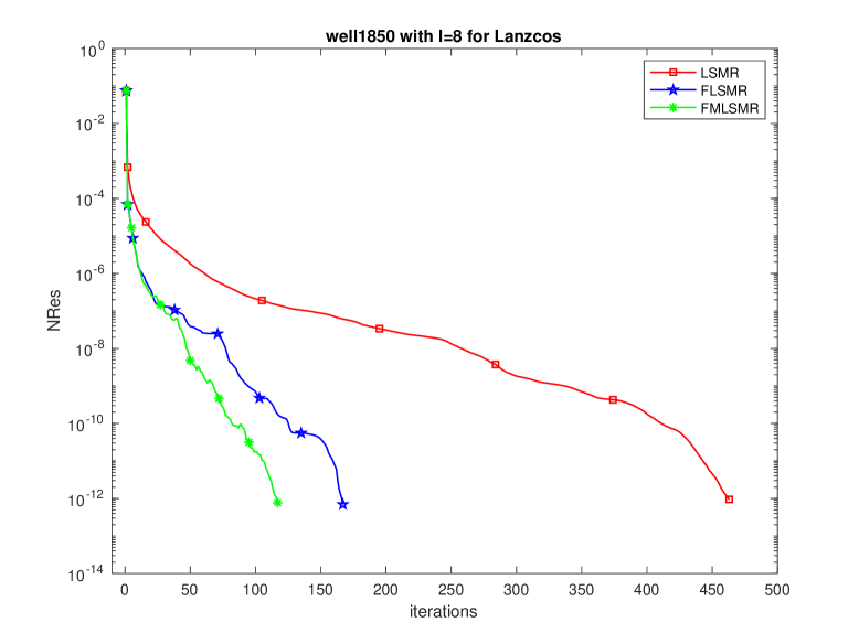
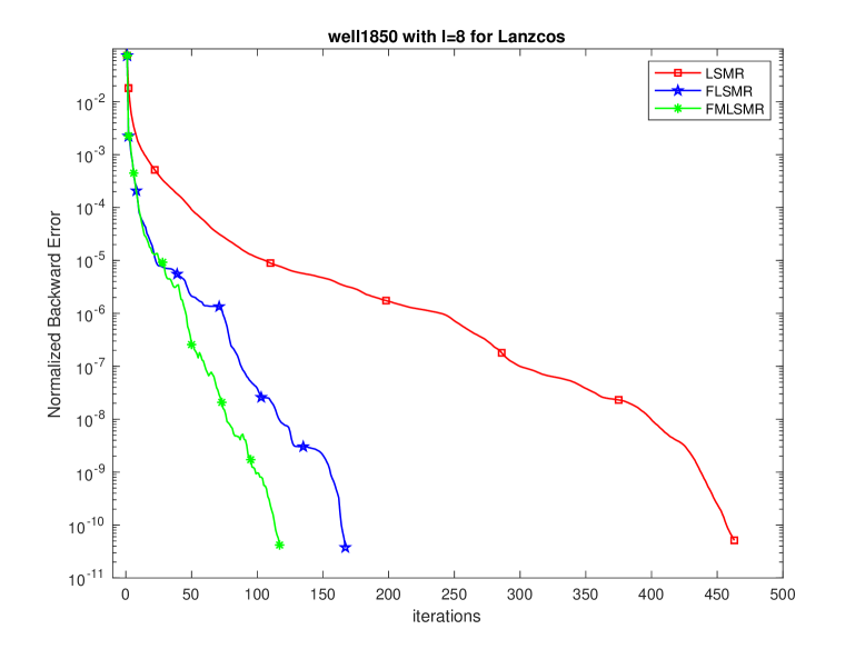
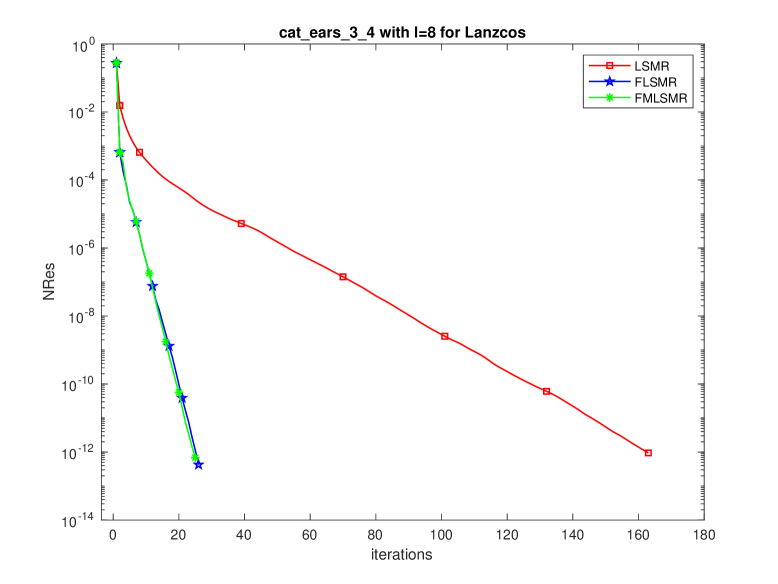
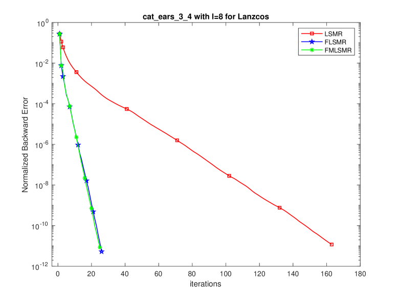
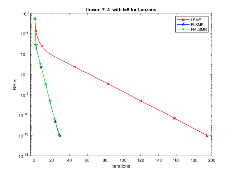
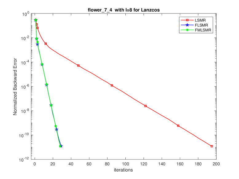
Figure 4.1: NRes (left panel) and normalized backward error $\|\hat{E}\|_{2}/\|A\|_{1}$ (right panel) for well1850, cat_ears_3_4, and flower_7_4.

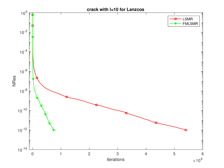
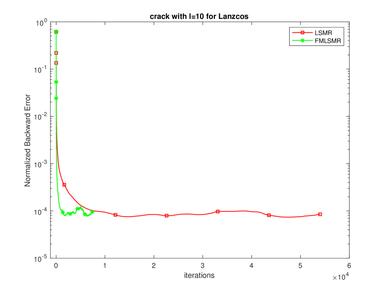
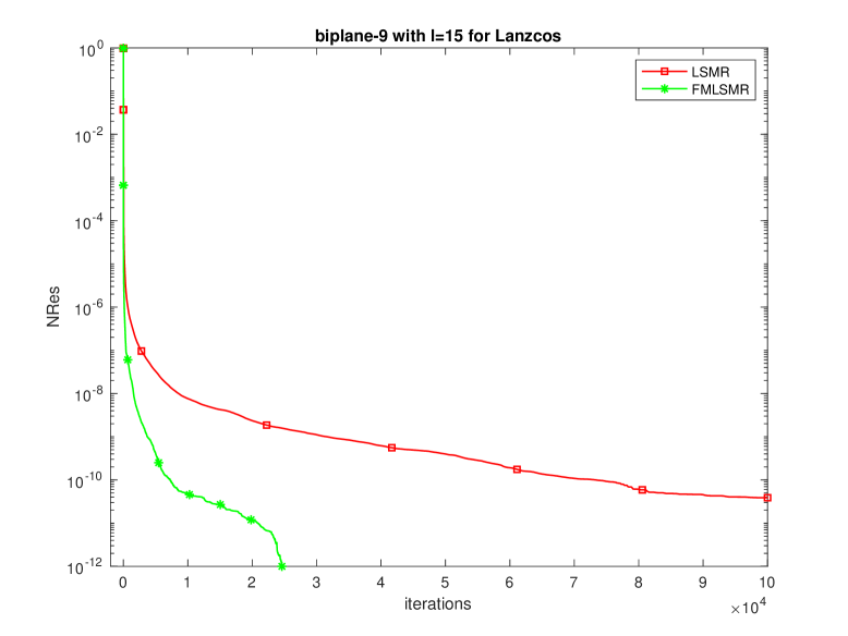
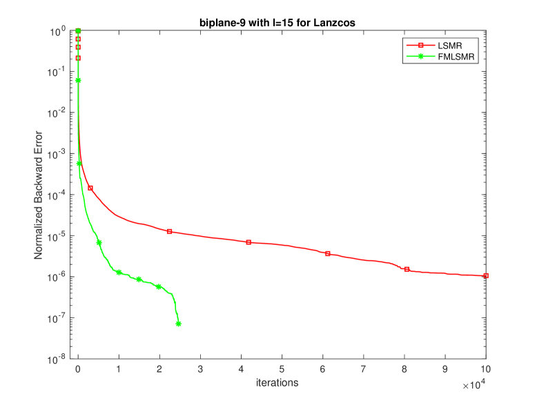
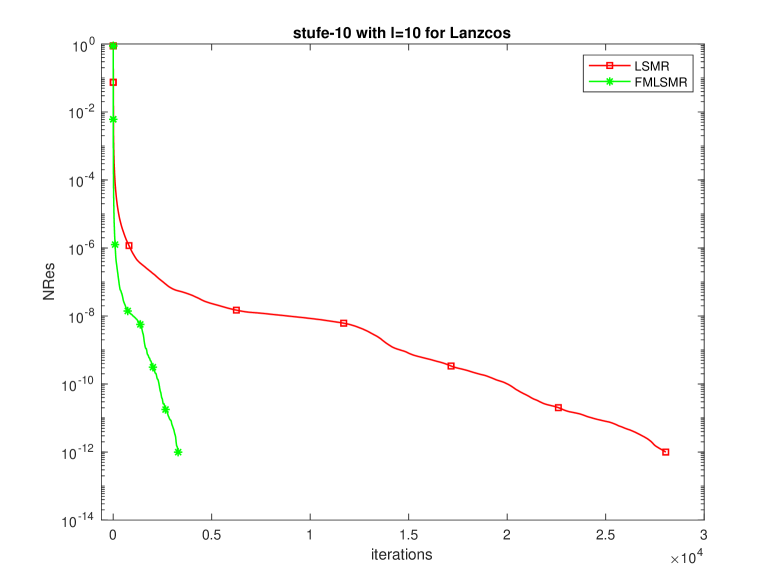
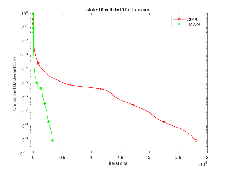
Figure 4.2: NRes (left panel) and normalized backward error $\|\hat{E}\|_{2}/\|A\|_{1}$ (right panel) for crack, biplane-9, and stufe-10.

We have the following observations from Table  4.4 and 4.5, and Figures 4.1 and 4.2.

• The FMLSMR can solve all eight problems while LSMR succeeds on five of them and FLSMR on only three. Overall, FMLSMR has the best performance in terms of iteration numbers and CPU times, except for well11850 on which both FLSMR and FMLSMR and fast while FLSMR holds an edge. Specifically, for well11850 and stufe-10, LSMR and FMLSMR has comparable performance in computational time. For cat_ears_3_4 and flower_7_4, FMLSMR is better than LSMR in terms of the number of iterations and CPU time. On delaunay_n16, biplane-9, fe_body, brack2, and stufe-10, FLSMR fails to satisfies the stopping criteria even for hours. According to Table 4.2, as the number of iterations increase, FLSMR uses much more storage and spends more on orthogonalization. The plots in the left column of Figures 4.1 and 4.2 demonstrate a consistent decrease in relative residual across all methods. Notably, FMLSMR exhibits the fastest convergence among all. Therefore, considering the storage advantage of FMLSMR and its simple implementation, we can say that FMLSMR is a very good choice, especially for difficult problems, over FLSMR and LSMR.

• The plots in the right column of Figures 4.1 and 4.2 show backward errors (4.3) for selective problems, and they display very similar patterns to that of NRes (4.1). Both $\|\hat{E}^{\rm FMLSMR}\|$ and $\|\hat{E}^{\rm FLSMR}\|$ are less than $\|\hat{E}^{\rm LSMR}\|$, which indicates FMLSMR and FLSMR compute more accurate solutions than LSMR does for the same number of iterations.

5 Conclusion

In this paper, we present a new method, the Flexible Modified LSMR (FMLSMR), which integrates the key ideas from the Modified LSMR and Flexible GMRES algorithms. We conduct a theoretical analysis of the Modified LSMR and compare it with the Flexible LSMR (FLSMR) when using a given fixed preconditioner. Through numerical experiments, we illustrate the efficiency of FMLSMR from various angles. The advantages of our method in terms of storage and computational cost position it as a promising numerical method for tackling challenging problems in practical applications.

References

- [1] S. R. Arridge, M. M. Betcke, and L. Harhanen. Iterated preconditioned LSQR method for inverse problems on unstructured grids. Inverse problem, 30(7):1–27, 2014.
- [2] H. Avron, E. Ng, and S. Toledo. Using perturbed QR factorizations to solve linear least squares problems. SIAM J. Matrix Anal. Appl., 31(2):674–693, 2009.
- [3] A. H. Baker, E. R. Jessup, and T. Manteuffel. A technique for accelerating the convergence of restarted GMRES. SIAM J. Matrix Anal. Appl., 26(4):962–984, 2005.
- [4] Å. Björck. Numerical Methods For Least Squares Problems. SIAM, Philadephia, 1996.
- [5] J. Chung and S. Gazzola. Flexible Krylov methods for regularization. SIAM J. Sci. Comput., 41(5):S149–S171, 2019.
- [6] D. C.-L. Fong and M. A. Saunders. LSMR: an iterative algorithm for sparse least-squares problems. SIAM J. Sci. Comput., 33(5):2950–2971, 2011.
- [7] L. Giraud, S. Gratton, X. Pinel, and X. Vasseur. Flexible GMRES with deflated restarting. SIAM Journal on Scientific Computing, 32(4):1858–1878, 2010.
- [8] G. Golub and W. Kahan. Calculating the singular values and pseduo-inverse of a matrix. SIAM J. Numer. Anal. Ser. B, 2(2):205–224, 1965.
- [9] N. J. Higham. Accuracy and Stability of Numerical Algorithms. SIAM, Philadephia, 2nd edition, 2002.
- [10] A. Imakura, R.-C. Li, and S. L. Zhang. Locally optimal and heavy ball GMRES methods. Japan J. Indust. Appl. Math., 33:471–499, 2016.
- [11] G. Karaduman and M. Yang. An alternative method for SPP with full rank (2, 1)-block matrix and nonzero right-hand side vector. Turkish Journal of Mathematics, 46(4):1330–1341, 2022.
- [12] G. Karaduman, M. Yang, and R.-C. Li. A least squares approach for saddle point problems. Japan Journal of Industrial and Applied Mathematics, 40(1):95–107, 2023.
- [13] N. Li and Y. Saad. MIQR: A mutilevel incomplete QR preconditioner for large sparse least-squares problems. SIAM J. Matrix Anal. Appl., 28(2):524––550, 2006.
- [14] K. Morikuni and K. Hayami. Convergence of inner-iteration GMRES methods for rank-deficient least squares problems. SIAM J. Sci. Comput., 36(1):225–250, 2015.
- [15] C. C. Paige and M. A. Saunders. LSQR: An algorithm for sparse linear equations and sparse least squares. ACM Trans. Math. Software, 8(1):43–71, 1982.
- [16] Y. Saad. A flexible inner-outer preconditioned GMRES algorithm. SIAM J. Sci. Comput., 14(2):461–469, 1993.
- [17] Y. Saad. Iterative Methods for Sparse Linear Systems. SIAM, Philadephia, 2nd edition, 2003.
- [18] G. W. Stewart. Research development and LINPACK. In J. R. Rice, editor, Mathematical Software III, pages 1–14. Academic Press, 1977.
- [19] B. Waldén, R. Karlson, and J.-G. Sun. Optimal backward perturbation bounds for the linear least squares problem. Numerical Linear Algebra with Applications, 2(3):271–286, 1995.
- [20] M. Yang. Optimizing Krylov Subspace Methods for Linear Systems and Least Squares Problems. PhD thesis, University of Texas at Arlington, UTA, 2018.
- [21] M. Yang and R.-C. Li. Heavy ball flexible GMRES method for nonsymmetric linear systems. Journal of Computational Mathematics, 40(5):715–730, 2022.