Universal mechanistic rules for de novo design of enzymes

Abstract

Enzymes are nano-scale machines that have evolved to drive chemical reactions out of equilibrium in the right place at the right time. Thermodynamically favourable reactions such as ATP hydrolysis are used by the cell to convert chemical energy into useful structure, function, and mechanical work. This includes the ‘fuelled’ catalysis of chemical reactions that would otherwise be thermodynamically unfavourable. Given the complexity and specificity of enzymatic function, bottom-up design of enzymes presents a daunting task that is far more challenging than making passive molecules with specific binding affinities or building nano-scale mechanically active devices. Here, we present a thermodynamically-consistent model for the operation of such a fuelled enzyme, which uses the energy from a favourable reaction to undergo non-equilibrium conformational changes that in turn catalyze a chemical reaction on an attached substrate molecule. We show that enzymatic function can emerge through a bifurcation upon appropriate implementation of momentum conservation on the effective reaction coordinates of the low dimensional description of the enzyme, and thanks to a generically present dissipative coupling. By considering the different aspects of the dynamics, such as the interplay of the non-equilibrium drive and the geometry of the enzyme-substrate complex, we propose three golden rules that should be universally applicable for de novo design of enzymes, as they are based on generic ingredients and physical constraints. These rules lead to optimal combinations of parameters, which can vastly accelerate reactions, while at the same time decreasing the energy dissipation of the combined reaction process, or, in other words, to an efficient enzyme. Our results can complement the recently developed strategies for de novo enzyme design based on machine learning approaches.

I Introduction

A fundamental question at the core of many areas of research is how to develop novel strategies for achieving non-equilibrium control at the nano-scale over the direction of chemical reactions [1]. While this is a challenging task from the point of view of bottom-up synthetic approaches, there are lessons to be learned from biological enzymes that have evolved to carry out such tasks with a high degree of precision and robustness despite the overwhelming buffeting by the environment in which they function. Since the pioneering work by Michaelis and Menten who elucidated some of the key phenomenological aspects of enzyme-assisted reaction kinetics [2, 3], our understanding of the underlying mechanisms behind these processes has been progressively refined [4, 5, 6, 7]. The underlying physical picture provided by the Kramers theory of noise-activated barrier crossing has provided a key conceptual framework for a reduced low-dimensional characterization of catalytic processes along appropriately selected reaction coordinates [8, 9], while molecular dynamics (MD) simulations of enzymes have been developing rapidly with the help of increased computing power [10].

All-atom MD approaches give important insight at the microscopic level, for particular systems of interest. However, they deal with many degrees of freedom and simulation parameters (e.g. atomic force fields), which might not readily lend themselves to the goal of extracting intuitive, minimal guidelines for the de novo design and optimization of enzymes. There is moreover still a large gap in time scales that can be computationally afforded to simulate sizeable numbers of catalytic cycles for most enzymes [11]. With the advent of machine learning approaches that are increasingly used in the design and optimization of enzymes [12, 13, 14], it is evident that such minimal design rules, which reflect the physical constraints on the conformational dynamics of proteins while driven away from equilibrium through catalytic activity, will be of great potential promise.

In recent years, fundamental insight from statistical physics has been successfully used towards experimental demonstrations of many interesting non-equilibrium phenomena [15, 16, 17, 18]. To aim towards the development of systems that can accomplish relatively complex tasks, one can benefit from innovative ideas that build on emergent physical properties of many-body non-equilibrium systems. Recent examples of such developments include proposals to employ non-reciprocal interactions to design collective barrier-crossing strategies that could emulate enzymatic function at larger scales [19], autonomous multifarious self-organization of complex protein structures [20], as well as proposed scenarios for fast and efficient self-organization of primitive metabolic cycles at the early stages of life formation [21].

The non-equilibrium dynamics of an enzyme during catalysis simultaneously involves energy transduction and conformational changes [22, 23], i.e. displacements. This suggests that mechanical considerations should play a key role in the stochastic dynamics of an enzyme, and consequently, in its optimal design with the aim of achieving the desired catalytic cycle. In other words, the mechanical activity of enzymes that lies at the core of their function as efficient catalysts bears a strong resemblance to the dynamics of molecular motors [24, 25, 26], with the important difference that the output energy is not in the form of mechanical work. Just like in the development of synthetic nano-motors, e.g. DNA-origami-based prototypes [18, 27, 28], it would be desirable to have bottom-up strategies to build synthetic enzymes.

Here, we set out to construct a minimal model for a ‘fuelled’ enzyme, so that we can extract a set of golden rules regarding its optimal design (see below). Our theoretical framework is built upon two main pillars, namely, momentum conservation as a fundamental physical constraint on the effective reaction coordinates that span the relevant low dimensional configuration space of the system, and a generically present dissipative coupling between the different reaction coordinates, which we systematically derive from a microscopic model. The implementation of momentum conservation leads to the emergence of an effective mechanochemical coupling in the same spirit as models used in studies of stochastic nano-swimmers [29, 30, 31, 32] and enhanced diffusion of enzymes [33, 34], while the dissipative coupling has been recently used to show how enzyme pairs can cooperate by exhibiting synchronization and enhanced catalytic activity [35]. The two ingredients described above give rise to a bifurcation in the dynamical phase-portrait of the low dimensional configuration space, which enables enzymatic activity as an emergent feature of the dynamics, via a fundamentally novel mechanism not accessible to Kramers-like energy barrier-crossing descriptions in terms of reaction coordinates. Our work complements other studies that involve minimal models for studying enzymatic behaviour, often based on colloids interacting through short-ranged interaction potentials or bead-spring networks [36, 37, 38, 39, 40, 41], which have been shown to be able to describe the action of a ‘passive’ enzyme, namely, catalysts that can accelerate a process of interest in the thermodynamically favourable direction.

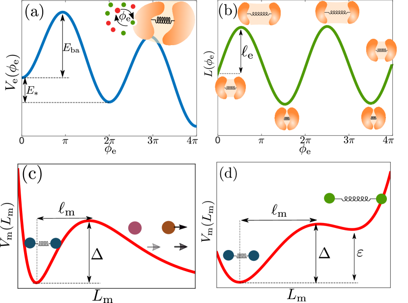
Figure 1: (a) The free energy landscape that drives the internal (fuel-to-waste) thermodynamically favourable reaction of the enzyme, where $E_{\mathrm{ba}}$ is the energy barrier height and $E_{*}$ the difference in the Gibbs free energy after a complete reaction. (b) The dynamics of the preferred length of the enzyme during the internal reaction, which induces conformational changes of amplitude $\ell_{\textrm{e}}$ during a reaction. (c, d) Free energy landscapes for the molecule, representing the thermodynamically unfavourable substrate-to-product reaction, for two examples of reaction: (c) dissociation of a dimer molecule into two monomers, (d) transition of a molecule between a short and a long conformational state. Here, $\Delta$ is the barrier height, $\varepsilon$ is the Gibbs free energy difference, and $\ell_{\textrm{m}}$ is the difference in the length of molecule between the initial and the transition state.

We consider an enzyme that undergoes conformational changes during the catalytic conversion of a fuel molecule to a waste molecule (Fig. 1(a,b) and Supplemental Videos 1 and 2). During each reaction, the enzyme undergoes an expansion and contraction cycle. We consider two types of substrate molecules: a dimer that can dissociate into two monomers (Fig. 1(c)), and a dimer that has two states, a short and a long one (Fig. 1(d) and Supplemental Video 3). In both cases, the dimer is attached at the outside of the enzyme. Through a detailed, thermodynamically consistent calculation, we show that during the fuel-induced contraction the enzyme can cause the dissociation of the dimer into monomers, or its transition from the short to the long conformation, respectively, even if these processes are not favoured thermodynamically or face a substantial energy barrier (see Supplemental Video 4). These catalyzed reactions are favourable in a large portion of the parameter space, related to the sizes and lengths of the enzyme and the bound molecule.

Our proposed dynamical paradigm, built on appropriate implementation of the relevant physical constraints on the minimal reaction coordinates, allows us to identify the following three golden rules for the optimal function of a fuelled enzyme driven by mechanochemical coupling: (i) the enzyme and the molecule should be attached at the smaller end of each; (ii) the conformational change of the enzyme must be comparable to or larger than the conformational change required of the molecule; (iii) the conformational change of the enzyme must be fast enough so that the molecule actually stretches, rather than just following the enzyme without stretching. The rules can provide useful input to the complementary perspectives of de novo enzyme design based on machine learning and all-atom simulations.

The article is organized as follows. We first present the enzyme-molecule model. After coarse-graining, we derive the general form of the dynamical equations of the enzyme and molecule. After introducing the relevant geometric parameters and energy landscapes, we study the corresponding deterministic dynamical system. We show that the catalytic action of the enzyme can be understood as emerging, in the mathematical language of dynamical systems theory, from a novel global bifurcation in the deterministic phase-space dynamics. This bifurcation is a consequence of the non-equilibrium drive of the fuel-to-waste reaction and the mechanochemical coupling with the passive molecule arising from enzyme conformational changes. We confirm the latter through the analysis of the stochastic dynamics in the presence of thermodynamically consistent noise. By studying the non-equilibrium steady-state of the system, we show the existence of an optimal set of parameters. Finally, an analysis of first-passage times shows that fuelled catalysis enables a great reduction of the characteristic reaction time and thus a substantial enhancement in the reaction rate.

II Model

In biological cells, many reactions are driven by enzymes that use a thermodynamically favourable reaction (fuel-to-waste) to power a thermodynamically unfavourable reaction (substrate-to-product) that would normally (spontaneously) take place in the opposite direction, in the absence of the enzyme. The most common fuel for these reactions is ATP, which is converted into useful work or motion [42, 26, 43, 44, 45]. Here we develop a minimal model to describe the dynamics of a fuelled enzyme.

II.1 Geometry and deterministic dynamics

We start with the simple model for an enzyme that undergoes conformational changes during catalysis, as previously introduced in Ref. 35. In particular, the fuel-to-waste reaction is not modelled explicitly, and is instead described by an internal phase $\phi_{\textrm{e}}$ which moves stochastically along a downhill washboard potential $V_{\textrm{e}}(\phi_{\textrm{e}})$; see Fig. 1(a). A noise-activated jump over one of the energy barriers (of height $E_{\mathrm{ba}}$) leads to an increase of the internal phase $\phi_{\textrm{e}}$ by $2\pi$, and corresponds to the conversion of fuel into waste with a free energy release given by $E_{*}$. We assume that the catalytic process is reaction-limited, which is equivalent to fuel molecules being sufficiently abundant, such that a new fuel molecule would effectively bind instantly to the enzyme after a reaction allowing the process to be repeated again.

The enzyme is represented by two sub-units, with the separation $L_{\textrm{e}}$ between them representing the mechanical degree of freedom that is coupled to the internal chemistry. This coupling is described by the potential $U(L_{\textrm{e}},\phi_{\textrm{e}})=\frac{k}{2}(L_{\textrm{e}}-L(\phi_{\textrm{e}}))^{2}+V_{\textrm{e}}(\phi_{\textrm{e}})$, where the first term is a harmonic potential that couples the actual length $L_{\textrm{e}}$ to a preferred length $L(\phi_{\textrm{e}})$ that depends on the internal phase describing the fuel-to-waste reaction; see Fig. 1(b). As a consequence of this coupling, every time that a fuel-to-waste reaction occurs the enzyme undergoes a cyclic conformational change.

The dynamics of the dimer molecule is described by a single degree of freedom, which is the separation $L_{\textrm{m}}$ between its two monomers; see Fig. 1(c,d). To model the two different chemical reactions already described (dimer dissociation and short-to-long conformation switch), two different potentials $V_{\textrm{m}}(L_{\textrm{m}})$ that govern the length of the molecule are used. For convenience and to unify the notation in both cases, we express the dimer length as $L_{\textrm{m}}=L_{\textrm{m}}^{(0)}+\ell_{\textrm{m}}\phi_{\textrm{m}}$ where $L_{\textrm{m}}^{(0)}$ is the length in the dimer state or in the transition state between short and long, respectively, and $\ell_{\textrm{m}}$ is the length increase necessary to reach the transition state; see Fig. 1(c,d).

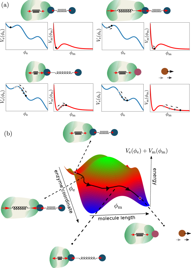
Figure 2: (a) A visualization of a dissociation process catalyzed by a fuelled enzyme, divided into four stages. The blue and red curves correspond to the energy landscape of the internal reaction of the enzyme $V_{\textrm{e}}(\phi_{\textrm{e}})$, and of the molecular reaction $V_{\textrm{m}}(\phi_{\textrm{m}})$, respectively. (b) The same process visualized within the two dimensional energy landscape given by $V_{\textrm{e}}(\phi_{\textrm{e}})+V_{\textrm{m}}(\phi_{\textrm{m}})$, where the black line shows the evolution of the combined enzyme-molecule system. Thermal noise tends to kick the system over the enzymatic energy barrier, since it is smaller than the barrier in the energy landscape of the molecule. The coupling between the enzyme and molecule dynamics, mediated by the conformational changes of the enzyme, then causes the system to cross over the energy barrier of the molecular reaction.

We now briefly describe the dynamics governing these degrees of freedom (for the detailed derivation see Appendix A). When the substrate molecule strongly binds to the enzyme, a complex effectively made up of three sub-units is formed (Fig. 2). Each sub-unit has a hydrodynamic mobility (inverse friction): $\mu_{\textrm{e}}$ for the part of the enzyme not bound to the molecule, $\mu_{\textrm{b}}$ for the unit that is shared by the molecule and the enzyme when bound to each other, and $\mu_{\textrm{m}}$ for the part of the molecule that is not bound to the enzyme. Since the typical time scales of the catalytic activity and the associated enzyme conformational transitions are much longer than the relevant inertial time scale [32], we consider the overdamped dynamics of these three sub-units, which leads to coupled evolution equations for the two lengths. Similarly, we consider overdamped dynamics for the evolution of the internal phase of the enzyme along the chemical free energy landscape, with an associated mobility $\mu_{\phi}$. By assuming that the enzyme is stiff, one can enslave the dynamics of the enzyme length (fast variable) onto the dynamics of the internal phase (slow variable). This reduces the degrees of freedom to two, and results in coupled equations for the internal phase of the enzyme and the length of the molecule. The deterministic components of the equations take on the form

$$\dot{\phi}_{\alpha}=\sum_{\beta=\textrm{e},\textrm{m}}M_{\alpha\beta}(\phi_{\textrm{e}})[-\partial_{\beta}V_{\beta}(\phi_{\beta})]$$ (1)

where $M_{\alpha\beta}$ is a symmetric effective mobility tensor (with $\alpha,\beta\in\{\textrm{e},\textrm{m}\}$), and $\partial_{\beta}\equiv\frac{\partial}{\partial\phi_{\beta}}$ (note that we do not implement a summation convention). The explicit expressions for the components of the mobility tensor are given as follows

$$M_{\textrm{e}\textrm{e}} =\frac{\mu_{\phi}}{1+\frac{\mu_{\phi}}{\mu_{1}}L^{\prime}(\phi_{\textrm{e}})^{2}},$$ (2)

$$M_{\textrm{e}\textrm{m}} =M_{\textrm{m}\textrm{e}}=-\bigg{(}\frac{\mu_{\phi}}{1+\frac{\mu_{\phi}}{\mu_{1}}L^{\prime}(\phi_{\textrm{e}})^{2}}\bigg{)}\frac{\mu_{\textrm{b}}}{\mu_{1}}\frac{L^{\prime}(\phi_{\textrm{e}})}{\ell_{\textrm{m}}},$$ (3)

$$M_{\textrm{m}\textrm{m}} =\frac{1}{{\ell_{\textrm{m}}}^{2}}\bigg{(}\mu_{2}-\frac{\mu_{\textrm{b}}^{2}}{\mu_{1}}\frac{1}{1+\frac{\mu_{\phi}}{\mu_{1}}L^{\prime}(\phi_{\textrm{e}})^{2}}\bigg{)},$$ (4)

where $\mu_{1}\equiv\mu_{\textrm{e}}+\mu_{\textrm{b}}$, $\mu_{2}\equiv\mu_{\textrm{m}}+\mu_{\textrm{b}}$, and $L^{\prime}(\phi_{\textrm{e}})=\frac{dL(\phi_{\textrm{e}})}{d\phi_{\textrm{e}}}$.

II.2 The effect of noise in the stochastic dynamics

Since enzymes operate at the nano-scale, they are strongly affected by the thermal fluctuations of the surrounding medium. In particular, because the dynamics is dissipative, thermal noise is essential to kick the system out of local energy minima and over barriers associated with the reactions; see Fig. 1(a,c,d).

Therefore, it is essential to introduce thermal fluctuations in our description of the problem. The system is out of equilibrium due to the driving force given by the energy $E_{*}$ of the fuel. In the limit of $E_{*}=0$, the steady state of the system must be a state of thermodynamic equilibrium, corresponding to a Boltzmann distribution. This implies that the stochastic dynamics corresponding to the deterministic dynamics in Eq. (1) must be described by a Fokker-Planck equation describing the time evolution of the probability distribution $P(\phi_{\textrm{e}},\phi_{\textrm{m}},t)$ as follows

$$\partial_{t}P+\sum_{\alpha=\textrm{e},\textrm{m}}\partial_{\alpha}J_{\alpha}=0,$$ (5)

with the conserved probability currents given as

$$J_{\alpha}(\phi_{\textrm{e}},\phi_{\textrm{m}},t)=\sum_{\beta=\textrm{e},\textrm{m}}M_{\alpha\beta}\big{[}P(-\partial_{\beta}V_{\beta})-k_{\rm B}T\partial_{\beta}P\big{]},$$ (6)

where $k_{\rm B}$ is the Boltzmann constant and $T$ is the temperature. In the absence of a non-equilibrium driving force ($E_{*}=0)$, both probability currents $J_{\mathrm{e}}$ and $J_{\mathrm{m}}$ must vanish at the equilibrium steady state. As a result, one recovers the Boltzmann distribution $P_{\mathrm{eq}}\propto\exp(-V_{\textrm{e}}(\phi_{\textrm{e}})/k_{\rm B}T)\exp(-V_{\textrm{m}}(\phi_{\textrm{m}})/k_{\rm B}T)$ independently of the form of the mobility matrix $M_{\alpha\beta}$, and thus of the geometric parameters describing the enzyme and the molecule.

That the equilibrium probability distribution factorizes reflects the fact that the two-dimensional energy landscape $V_{\textrm{e}}(\phi_{\textrm{e}})+V_{\textrm{m}}(\phi_{\textrm{m}})$ in which the phases evolve is separable, i.e. there is no coupling between $\phi_{\textrm{e}}$ and $\phi_{\textrm{m}}$ through the potential. The dynamics of $\phi_{\textrm{e}}$ and $\phi_{\textrm{m}}$ are coupled only through the off-diagonal components of the mobility tensor $M_{\alpha\beta}$, which arise due to the mechanical contact (binding) between enzyme and molecule in combination with the conformational changes of the enzyme, and represent a form of dissipative coupling which only plays a role in a non-equilibrium setting ($E_{*}>0$), i.e. when the fuel-to-waste reaction is thermodynamically favoured. This type of coupling has been seen to emerge in models of coupled molecular machines (via mechanical binding or hydrodynamic interactions mediated by a viscous fluid) and enables cooperative phenomena like synchronization [35, 46] and phase-locking [47] among enzymes, of which there is suggestive experimental evidence [48, 49].

The Langevin equation associated to the Fokker-Planck equation in Eq. (5) takes the following form in the Stratonovich convention,

$$\dot{\phi}_{\alpha}=\sum_{\beta=\textrm{e},\textrm{m}} \Big{[}M_{\alpha\beta}(-\partial_{\beta}V_{\beta})+\sqrt{2k_{\rm B}T}\sigma_{\alpha\beta}\xi_{\beta}$$

$$+\sum_{\nu=\textrm{e},\textrm{m}}k_{\rm B}T\sigma_{\alpha\nu}\partial_{\beta}\sigma_{\beta\nu}\Big{]},$$ (7)

where $\sum_{\nu=\textrm{e},\textrm{m}}\sigma_{\alpha\nu}\sigma_{\beta\nu}=M_{\alpha\beta}$. The term on the second line of the right hand side is the spurious drift term arising from the multiplicative nature of the noise, due to the dependence of the mobility matrix on $\phi_{\textrm{e}}$, while the last term on the first line of Eq. (7) is the thermal noise with $\xi_{\beta}$ being a unit white noise such that $\langle\xi_{\beta}(t)\rangle=0$ and $\langle\xi_{\alpha}(t)\xi_{\beta}(t^{\prime})\rangle=\delta_{\alpha\beta}\delta(t-t^{\prime})$. It is also worth noting that the mobility matrix must be symmetric and positive definite (which is the case here) in order for the dynamics to be thermodynamically consistent [50, 51].

Parameters			Description
$\mu_{\phi}$			mobility of the internal phase $\phi_{\textrm{e}}$ (reaction coordinate of fuel-to-waste reaction)
$\mu_{\textrm{e}}$			hydrodynamic mobility of the enzyme-only sub-unit
$\mu_{\textrm{m}}$			hydrodynamic mobility of the molecule-only sub-unit
$\mu_{\textrm{b}}$			hydrodynamic mobility of the shared (bound) sub-unit
$\mu_{1}=\mu_{\textrm{e}}+\mu_{\textrm{b}}$			sum of the mobilities of the enzyme-only and shared sub-units
$\mu_{2}=\mu_{\textrm{m}}+\mu_{\textrm{b}}$			sum of the mobilities of the molecule-only and shared sub-units
$h=\mu_{\textrm{b}}/(\mu_{\textrm{e}}+\mu_{\textrm{b}})$			effective coupling strength ($0\leq h\leq 1$)
$\ell_{\textrm{e}}$			amplitude of the conformational change of the enzyme
$\ell_{\textrm{m}}$			length difference between the initial and transition states of the molecule
$E_{\mathrm{ba}}$			energy barrier of the fuel-to-waste reaction
$E_{*}$			Gibbs free energy released by the fuel-to-waste reaction
$\Delta$			energy barrier of the molecule reaction
$\varepsilon$			unfavourable energetic bias of the short-to-long reaction
$k_{\rm B}T$			thermal energy (strength of thermal fluctuations)

Table 1: Summary of the parameters of the model.

II.3 Model parametrization

The enzyme and the molecule are embedded in a solvent under low Reynolds number conditions [51]. Therefore, we can infer that the mobilities $\mu_{\textrm{e}}$ (enzyme-only sub-unit), $\mu_{\textrm{b}}$ (bound enzyme-molecule sub-unit), and $\mu_{\textrm{m}}$ (molecule-only sub-unit) are related to their corresponding effective hydrodynamic radii $a_{\textrm{e}}$, $a_{\textrm{b}}$, and $a_{\textrm{m}}$, via the Stokes relation $\mu=1/(6\pi\eta a)$, ignoring hydrodynamic interactions in this lowest order approximation. The mobilities thus directly encode information about the sizes of the enzyme and the molecule sub-units. The length scale related to the amplitude of the deformation of the molecule is $\ell_{\textrm{m}}$; see Fig. 1(c,d). For the conformational changes of the enzyme, we assume that the preferred length $L(\phi_{\textrm{e}})$ oscillates during the enzymatic cycle as

$$L(\phi_{\textrm{e}})=L_{\textrm{e}}^{(0)}+\ell_{\textrm{e}}\sin(\phi_{\textrm{e}}-\delta),$$ (8)

where $L_{\textrm{e}}^{(0)}$ is an average length which does not enter the dynamics, $\ell_{\textrm{e}}$ is the amplitude of the conformational change, and $\delta$ is a phase shift described below (we choose $\ell_{\textrm{e}}\geq 0$).

The washboard potential governing the dynamics of the internal phase $\phi_{\textrm{e}}$ is taken to be of the form $V_{\textrm{e}}(\phi_{\textrm{e}})=-F\phi_{\textrm{e}}+v\sin(\phi_{\textrm{e}}-\delta)$ where $\delta=\arccos(F/v)$ is the value of the phase shift which guarantees that the minima of the potential are located at integer multiples of $2\pi$. The parameters $F$ and $v$ can be mapped to the height of the energy barrier of the enzymatic reaction $E_{\mathrm{ba}}$ and the free energy released after a complete reaction $E_{*}$ (see Fig. 1(a)) through $E_{\mathrm{ba}}=[2\sqrt{1-(F/v)^{2}}+2\delta(F/v)]v$ and $E_{*}=2\pi F$ [35, 47, 52]. By eliminating $v$ and $F$, we find that the parameter $\delta$ is given by the solution of the transcendental equation

$$\delta+\tan\delta=\pi E_{\mathrm{ba}}/E_{*},$$ (9)

which yields the approximate solution

$$\delta\simeq\frac{\pi}{2}\frac{E_{\mathrm{ba}}}{E_{*}},$$ (10)

for small values of $E_{\mathrm{ba}}/E_{*}$.

The parameter $\mu_{\phi}$ is the mobility of the internal phase $\phi_{\textrm{e}}$ and may have different microscopic origins depending on the particulars of the fuel-to-waste reaction. In principle, it can be related to the rate $k_{\mathrm{cat}}$ of the catalytic reaction and the height of the energy barrier $E_{\mathrm{ba}}$ through the Kramers escape rate [8, 9]

$$k_{\mathrm{cat}}=\frac{\mu_{\phi}}{2\pi}\sqrt{\lvert\lambda\rvert\lambda^{(0)}}\exp\bigg{(}-\frac{E_{\mathrm{ba}}}{k_{\rm B}T}\bigg{)},$$ (11)

where $\lambda^{(0)}=V_{\textrm{e}}^{\prime\prime}|_{\rm min}$ and $\lambda=V_{\textrm{e}}^{\prime\prime}|_{\rm max}$, i.e. they correspond to the values of the second derivative (curvature) of the potential around the minimum and the maximum (energy barrier), respectively. Thus, by knowing the catalytic rate and barrier height of a reaction one can infer the value of $\mu_{\phi}$.

For the molecule, we consider two different types of reaction starting from a dimer-like substrate. For the dissociation reaction, we consider a potential with a minimum representing the stable initial state of the molecule, a maximum corresponding to an energy barrier with height $\Delta$, and an asymptotic decrease to a constant value, which represents the fact that beyond the barrier the monomers become disconnected. We describe this with the potential $V_{\textrm{m}}(\phi_{\textrm{m}})=\Delta\phi_{\textrm{m}}^{2}\exp[2(1-\phi_{\textrm{m}})]$, shown in Fig. 1(c). For the conformational switch reaction where the dimer switches from a short to a long state, we choose a bistable potential, with an energy barrier $\Delta$ and an energy difference $\varepsilon$ between the long (higher energy) and the short (lower energy) states. We model this using the potential $V_{\textrm{m}}(\phi_{\textrm{m}})=\Delta\phi_{\textrm{m}}^{2}(\phi_{\textrm{m}}^{2}-2)+\varepsilon\phi_{\textrm{m}}/2$, with $\varepsilon<\Delta$; see Fig. 1(d). All the relevant model parameters are summarized in Table 1.

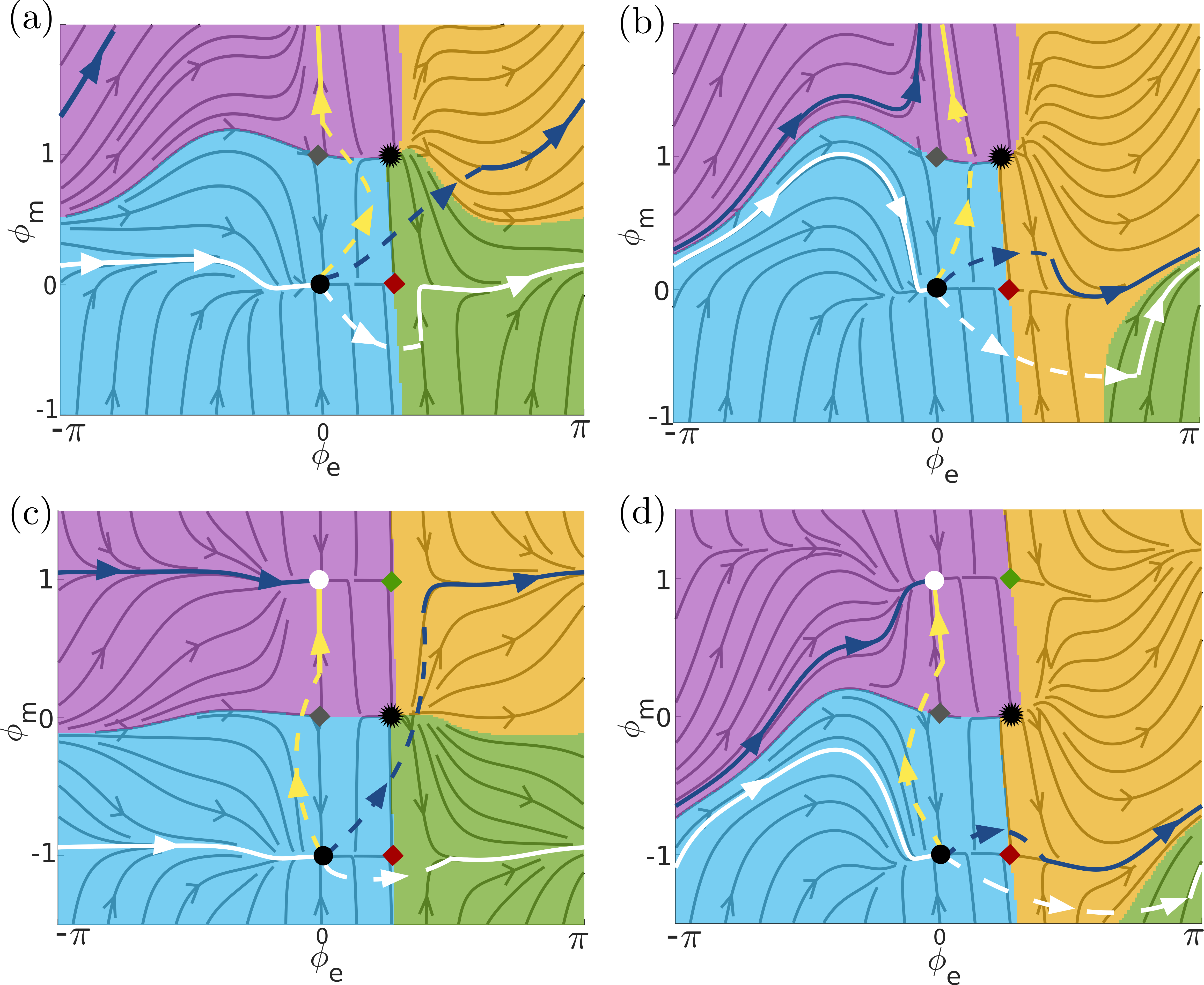
Figure 3: Phase-portraits of the deterministic dynamics for (a,b) the dissociation reaction and (c,d) the switch reaction. A global bifurcation occurs with increasing coupling strength $h$, which is below the critical value in (a,c) and above it in (b,d). In all cases, stable fixed points are depicted as circles, saddle points as diamonds, and unstable fixed points as asterisks. Dashed lines depict possible scenarios in which thermal fluctuations can kick the system out of the basin of attraction of a stable fixed point. The solid flow lines show typical trajectories, and their final resting points, when starting from different basins of attraction. The different colouring of the diamonds is described in the text. The values of the coupling are (a) $h=0.33$, (b) $h=0.48$, (c) $h=0.12$, and (d) $h=0.48$.

III Results

III.1 Preliminary considerations

It is crucial to note that the components of the mobility tensor $M_{\alpha\beta}$ are determined by the geometric features of the enzyme and molecule, which can be tuned as to optimize the function of the enzyme. The basic principle is illustrated in Fig. 2(a), for the example of dissociation of a dimer molecule. When a catalytic reaction takes place (the internal phase $\phi_{\textrm{e}}$ is kicked over the chemical energy barrier by thermal noise), the coupling to the molecule length arising from the conformational changes of the enzyme drives a corresponding evolution of the molecule length, as represented by $\phi_{\textrm{m}}$, and in particular can cause $\phi_{\textrm{m}}$ to overcome its energy barrier. The evolution along the two-dimensional energy landscape $V_{\textrm{e}}(\phi_{\textrm{e}})+V_{\textrm{m}}(\phi_{\textrm{m}})$ is shown in Fig. 2(b), where the black path corresponds to a catalyzed reaction.

We expect to have a strong coupling between the fuel-to-waste ($\phi_{\textrm{e}}$) and substrate-to-product ($\phi_{\textrm{m}}$) reactions when the off-diagonal components in the mobility tensor are non-negligible. In the limiting cases where either the middle sub-unit is large compared to the enzyme-only sub-unit, $\mu_{\textrm{b}}/\mu_{1}\rightarrow 0$, or the conformational changes of the enzyme are small compared to the dissociation length of the molecule, $\ell_{\textrm{e}}/\ell_{\textrm{m}}\rightarrow 0$, the off-diagonal terms vanish, leading to a decoupling of the dynamics between the enzyme and the molecule. To achieve a strong coupling, we would aim to maximize $\mu_{\textrm{b}}/\mu_{1}$ and $\ell_{\textrm{e}}/\ell_{\textrm{m}}$, from which one can infer the first two golden rules [(i) and (ii)] for designing an enzyme discussed above. In the following, we define the ratio $h\equiv\mu_{\textrm{b}}/\mu_{1}=\mu_{\textrm{b}}/(\mu_{\textrm{e}}+\mu_{\textrm{b}})$ to be the “coupling strength”, and we note that it is bounded as $0\leq h\leq 1$. For $h<0.5$, the mobility of the shared sub-unit is larger than that of the enzyme-only sub-unit, and the reverse is true for $h>0.5$.

Throughout the rest of the text we will use the following parameters unless mentioned otherwise: $\mu_{\phi}\ell^{2}_{\textrm{m}}/\mu_{2}=1$, $\ell_{\textrm{e}}/\ell_{\textrm{m}}=2.5$, $\mu_{1}/\mu_{2}=0.88$, $E_{*}/\Delta=14\pi$, $E_{\mathrm{ba}}/\Delta=0.4$, and (for the switch reaction) $\varepsilon/\Delta=0.1$. The dimensionless time is defined as $\tilde{t}=(\mu_{\phi}\Delta)t$. The remaining dimensionless parameters that we explore in the text are the coupling strength $h$ and the dimensionless thermal noise strength $k_{\rm B}T/\Delta$.

III.2 Deterministic dynamics and global bifurcation

Before considering the full stochastic (noise-activated) dynamics of the system, we first study the deterministic dynamics given by Eq. (1), as we can apply tools from dynamical systems theory to obtain an intuitive understanding of the expected behaviour, particularly in the experimentally-relevant case of low noise, where $k_{\rm B}T$ is smaller than all other energy scales.

In Fig. 3, phase portraits of the deterministic dynamics are shown for low and high coupling strengths and both types of reaction (see Appendix C for details of the numerical calculation of phase portraits). Depending on the type of reaction, different sets of fixed points appear in the dynamics (stable fixed points are depicted as circles, saddle points as diamonds, and unstable fixed points as asterisks). For the dissociation reaction, there are four fixed points (one stable, two saddle points, one unstable) since there is no local minimum of the molecule potential after the energy barrier. The stable fixed point at $\phi_{\textrm{m}}=0$ corresponds to the substrate (dimer) state, whereas $\phi_{\textrm{m}}\to\infty$ corresponds to the product (dissociated) state. For the switch reaction, there are six fixed points (two stable, three saddle points, one unstable). The stable fixed point at $\phi_{\textrm{m}}=-1$ corresponds to the substrate (short) state, whereas that at $\phi_{\textrm{m}}=+1$ corresponds to the product (long) state. It is worth noting that the positions of the fixed points do not depend on the coupling, but only on the potentials $V_{\textrm{e}}(\phi_{\textrm{e}})$ and $V_{\textrm{m}}(\phi_{\textrm{m}})$. Thus, changes in the geometry of the enzyme-molecule complex (and thus in the coupling strength) leave the location and nature of the fixed points unchanged. As a consequence, there cannot be any local bifurcations in the dynamical system and only global bifurcations are allowed [35]. By considering the topology of the different basins of attraction in the dynamical system, we note that global bifurcations occur between Figs. 3(a) and 3(b) for the dissociation reaction, and between Figs. 3(c) and 3(d) for the switch reaction, respectively.

The phase portraits allow us to uncover the different possibilities emerging in the full stochastic dynamics by classifying the different types of possible deterministic trajectories, depicted as solid flow lines in Fig. 3, and considering the likelihood of their stochastic activation by random thermal kicks, depicted as dashed flow lines in Fig. 3, which will take the system from an initial state around a stable fixed point to the domain of interest. Trajectories starting in the cyan region in Fig. 3 are attracted to the fixed point at $(\phi_{\textrm{e}},\phi_{\textrm{m}})=(0,0)$ (for the dissociation reaction) or $(0,-1)$ (for the switch reaction). On the other hand, those starting in the green region are attracted to the fixed point at $(\phi_{\textrm{e}},\phi_{\textrm{m}})=(2\pi,0)$ (dissociation) or $(2\pi,-1)$ (switch). This class of trajectories, which are depicted as solid white flow lines in Fig. 3, represent the process in which the molecule remains in the substrate state and the enzyme performs a futile cycle. Analogously, trajectories starting in the magenta region end at $(0,\infty)$ (dissociation) or $(0,1)$ (switch), corresponding to spontaneous transition of the molecule to the product state, without an accompanying transition in the enzyme, while those in the orange region converge to $(2\pi,\infty)$ (dissociation) or $(2\pi,1)$ (switch), representing a process in which the molecular transition coincides with the enzymatic cycle. The relative frequency of the activation of the different processes corresponding to these distinct classes will depend on the likelihood of the availability of the thermal kick of the right strength that is needed to initiate each of them.

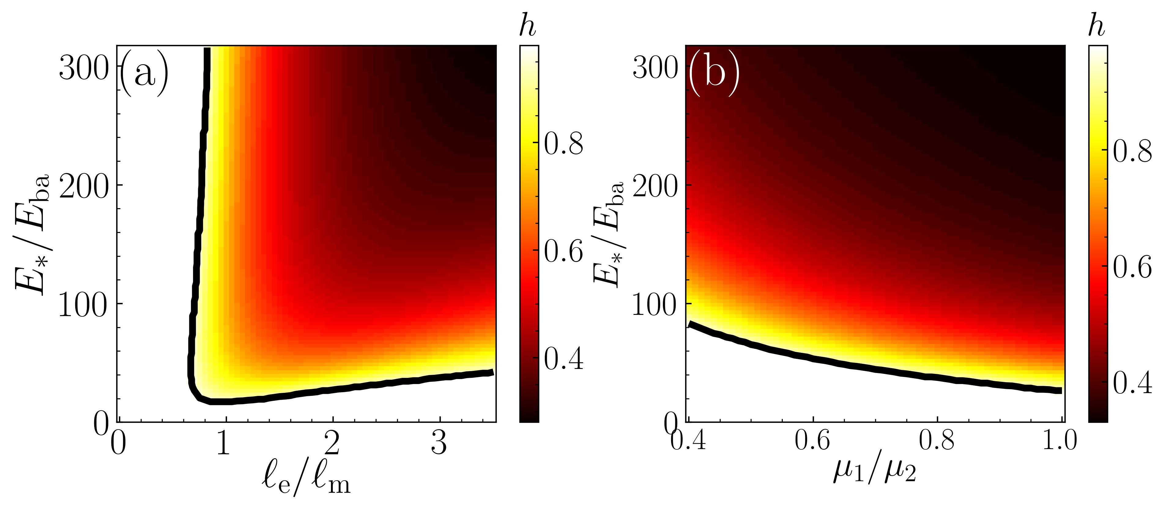
Figure 4: Critical coupling strength at which the bifurcation occurs, as a function of (a) the geometric ratio $\ell_{\textrm{e}}/\ell_{\textrm{m}}$ and the ratio $E_{*}/E_{\mathrm{ba}}$ describing the internal enzyme reaction, and (b) the mobility ratio $\mu_{1}/\mu_{2}$ and $E_{*}/E_{\mathrm{ba}}$. In the white region outside the black solid line, a bifurcation does not occur within the physical range $0\leq h\leq 1$.

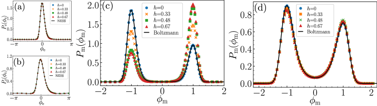
Figure 5: Marginal steady-state distributions for the switching reaction, (a,c) at low noise $k_{\rm B}T/\Delta=0.15$, and (b,d) at high noise $k_{\rm B}T/\Delta=0.4$. The distribution for the enzyme coordinate $\phi_{\textrm{e}}$ is shown in (a,b), and that for the molecule coordinate $\phi_{\textrm{m}}$ in (c,d). In (a,b) the black line labelled “NESS” is the analytical result for an uncoupled enzyme given in Eq. (D). In (c,d) the black line labelled “Boltzmann” is the equilibrium distribution $P_{\textrm{m}}(\phi_{\textrm{m}})\propto\exp(-V_{\textrm{m}}/k_{\rm B}T)$.

More specifically, let us consider the case of weak coupling in Figs. 3(a,c). Thermal fluctuations can most likely kick the system over one of the two saddle points or transition states, either the one to the right of the stable fixed point shown as red diamond (white trajectory) or the one above it shown as grey diamond (yellow trajectory). When traversing the red diamond, the enzyme will complete an internal reaction ending at $\phi_{\textrm{e}}=2\pi$, while the molecule remains in the substrate state. When traversing the grey diamond, the molecule undergoes a reaction and turns into product, while the enzyme completes no internal reaction and remains at $\phi_{\textrm{e}}=0$. Thus, the internal (fuel-to-waste) reaction of the enzyme and the molecule (substrate-to-product) reaction are completely uncoupled in these cases. Less likely thermal fluctuations can kick the system across the unstable fixed point shown as asterisk (blue trajectory), leading to a simultaneous occurrence of both the enzyme and the molecule cycles.

We next consider the case of strong coupling, after the global bifurcation has occurred and the basins of attraction have rearranged; see Fig. 3(b,d) and Supplemental Videos 5 and 6. Thermal fluctuations kicking the system over the grey diamond (yellow trajectory) will still result in molecular reactions without associated internal reactions in the enzyme. However, if the system is activated over the red diamond, the more likely scenario will be for the enzyme to complete an internal reaction simultaneously with the molecular reaction (blue trajectory) unlike in the weak coupling case. The two reactions thus become coupled, and in particular, a fuel-to-waste reaction inside the enzyme now triggers a substrate-to-product reaction for the molecule. The futile enzyme cycle (white trajectory) is the more unlikely scenario in this case. We note that a similar bifurcation occurs for the reverse switching process, where the energetically favourable and initial state for the molecule is the long conformation; see Appendix B.

The bifurcation occurs above a critical value of the coupling $h$, which can be tuned by the geometric properties of the enzyme-substrate complex. Moreover, in order to have an enzyme-triggered reaction, transitions through the red diamond should be favoured over transitions through the grey diamond. This is expected to happen when the energy barrier for the internal reaction is smaller than that of the molecular reaction ($E_{\mathrm{ba}}<\Delta)$. It is also worth mentioning that, even though the dissociation and switch reactions involve rather different energy landscapes, the bifurcation takes place at the same set of parameters since in both cases the barrier for the molecular reaction is fixed to $\Delta$.

The occurrence of the bifurcation is crucial for the coupling between the two processes to emerge, and thus for the enzyme to become active. We thus explore how the critical coupling depends on the geometric and energetic parameters of the enzyme-substrate complex. In Fig 4, we show the critical value of the coupling $h$ as a function of the ratio $E_{*}/E_{\mathrm{ba}}$ of energies in the fuel-to-waste reaction, and $\ell_{\textrm{e}}/\ell_{\textrm{m}}$ or $\mu_{1}/\mu_{2}$ which are directly related to the geometrical properties of the complex. In Fig 4(a), it is observed that the bifurcation takes place at low coupling strengths when the driving $E_{*}$ is large, which is linked to higher reaction rates [related to golden rule (iii)]. In addition, there is a non-trivial behaviour as a function of the length ratio $\ell_{\textrm{e}}/\ell_{\textrm{m}}$ at a fixed value of $E_{*}/E_{\mathrm{ba}}$, showing non-monotonic behaviour with a minimum at intermediate values. In Fig 4(b), we see that the bifurcation is favoured at higher values of the ratio $\mu_{1}/\mu_{2}$. The results in Fig. 4 serve to highlight the different parameters that must be tuned in order to favour a bifurcation in the deterministic dynamics. Below, we show how these results translate to the full noise-activated stochastic dynamics.

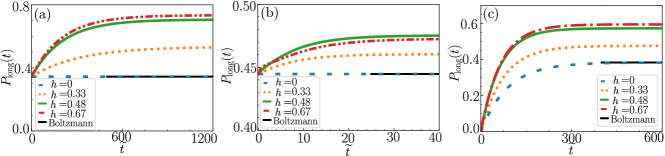
Figure 6: Probability of finding the shape-switching molecule in the long state as a function of time, for various values of the coupling $h$. In (a,b) the initial state is chosen as a Boltzmann distribution, while in (c) it is chosen as a narrow Gaussian centered around the short state. The strength of the noise is (a) $k_{\rm B}T/\Delta=0.15$, (b) $k_{\rm B}T/\Delta=0.4$, and (c) $k_{\rm B}T/\Delta=0.2$. The horizontal line labelled “Boltzmann” is the long-time limit expected from an equilibrium distribution.

III.3 Stochastic dynamics

III.3.1 Steady state: driving a reaction uphill

Passive enzymes can lower reaction barriers, but do not shift reaction equilibria, which are still purely governed by the free energy differences between substrate and product. Fuelled enzymes, on the other hand, can use the free energy provided by the fuel to drive the substrate-to-product reaction uphill, i.e. favouring the formation of a high free energy product from a low free energy substrate. To study whether our model enzyme is capable of driving reactions uphill, we focus on the switch reaction (Fig. 1(d)), and numerically solve the Fokker-Planck equation (Eq. (5), see Appendix C for details of the numerical solution), where we are interested in how the probability distribution evolves over time and in the form of the steady state distribution in the long time limit, where $\partial_{t}P_{\mathrm{ss}}\rightarrow 0$.

In Fig. 5, the steady state marginal distributions $P_{\textrm{e}}(\phi_{\textrm{e}})\equiv\int^{\infty}_{-\infty}d\phi_{\textrm{m}}P_{\mathrm{ss}}(\phi_{\textrm{e}},\phi_{\textrm{m}})$ and $P_{\textrm{m}}(\phi_{\textrm{m}})\equiv\int^{2\pi}_{0}d\phi_{\textrm{e}}P_{\mathrm{ss}}(\phi_{\textrm{e}},\phi_{\textrm{m}})$ for the enzyme and molecule reaction coordinates are presented for low and high thermal noise. Both at low and at high noise, the effect of the coupling $h$ is negligible with respect to the non-equilibrium steady state (NESS) attained by the enzyme, $P_{\textrm{e}}(\phi_{\textrm{e}})$; see Fig. 5(a,b). The form of $P_{\textrm{e}}(\phi_{\textrm{e}})$ can be obtained analytically in the $h=0$ case (solid black line), by extending a classical calculation [53, 54, 55] to the case with multiplicative noise, i.e. a phase-dependent mobility, as described in Appendix D. At high temperatures, the multiplicative noise causes a small maximum at intermediate values of $\phi_{\textrm{e}}$ that would not be present for additive noise; see Fig. 5(b).

In stark contrast, at low noise the coupling $h$ has a substantial effect on the NESS attained by the molecule, $P_{\textrm{m}}(\phi_{\textrm{m}})$; see Fig. 5(c). At $h=0$, the distribution $P_{\textrm{m}}(\phi_{\textrm{m}})$ corresponds to a Boltzmann distribution $\propto e^{-V_{\textrm{m}}(\phi_{\textrm{m}})/k_{\rm B}T}$, and thus shows two peaks (corresponding to the short and long states), with the peak corresponding to the lower energy short state being much higher. As the coupling $h$ increases, we see this trend progressively reverse, as the fuelled action of the enzyme drives more and more probability towards the long state. This demonstrates that the fuelled action of the enzyme can indeed drive a reaction uphill, in the thermodynamically unfavourable direction. However, the action of the enzyme becomes much less effective at high noise, where deviations from the Boltzmann equilibrium are minimal; see Fig. 5(d).

To further understand this effect, we consider the time evolution of the probability of finding the molecule in the long state $P_{\mathrm{long}}(t)$, defined as

$$P_{\mathrm{long}}(t)=\int^{2\pi}_{0}d\phi_{\textrm{e}}\int^{\infty}_{\phi_{\mathrm{m},\mathrm{max}}}d\phi_{\textrm{m}}P(\phi_{\textrm{e}},\phi_{\textrm{m}},t),$$ (12)

where $\phi_{\mathrm{m},\mathrm{max}}$ is the location of the energy barrier of the molecular reaction along the $\phi_{\textrm{m}}$ coordinate. We consider an enzyme and a molecule that are initially separated from each other, and bind at time $t=0$. We thus initialize the enzyme probability distribution as being in the steady state of an uncoupled enzyme ($h=0$). For the molecule, we consider two cases: (i) the molecule starts in its Boltzmann equilibrium, or (ii) the molecule starts only in the short state (with probability distributed in a narrow Gaussian around it). Results from numerical solution of the Fokker-Planck equation (Eq. (5)) are shown in Fig. 6. For $h=0$, $P_{\mathrm{long}}$ tends to the probability corresponding to the equilibrium Boltzmann distribution, as expected. However, for $h>0$, $P_{\mathrm{long}}$ is consistently higher than what the Boltzmann distribution dictates. Clearly, coupling to the fuelled enzyme can drive the molecular reaction uphill. The effect is most pronounced at larger coupling strengths and lower noise.

From $P_{\mathrm{long}}(t)$, we may calculate the probability that the molecule is in the long state once it unbinds from the enzyme, which is a quality measure for the function of the enzyme. Assuming that the molecule unbinds from the enzyme at a rate $k_{\mathrm{off}}$, the probability of the molecule remaining bound at time $t$ is $p_{\mathrm{bo}}(t)=\exp(-k_{\mathrm{off}}t)$. The probability of unbinding precisely between $t$ and $t+dt$ is then $p_{\mathrm{bo}}(t)k_{\mathrm{off}}dt$, and thus the average probability of being in the long state when it unbinds is

$$\langle P_{\mathrm{long}}\rangle=k_{\mathrm{off}}\int^{\infty}_{0}dt^{\prime}P_{\mathrm{long}}(t^{\prime})p_{\mathrm{bo}}(t^{\prime}).$$ (13)

The behaviour of $P_{\mathrm{long}}(t)$ in Fig. 6 can be well approximated by an exponential relaxation $P_{\mathrm{long}}(t)\simeq P_{\mathrm{long}}(\infty)-[P_{\mathrm{long}}(\infty)-P_{\mathrm{long}}(0)]\exp(-k_{\mathrm{cat}}t)$, where $k_{\mathrm{cat}}$ is the inverse timescale associated with the transient regime in Fig. 6. With this choice, Eq. (13) evaluates to

$$\langle P_{\mathrm{long}}\rangle\simeq\frac{k_{\mathrm{off}}P_{\mathrm{long}}(0)+k_{\mathrm{cat}}P_{\mathrm{long}}(\infty)}{k_{\mathrm{off}}+k_{\mathrm{cat}}}.$$ (14)

In the limiting case in which $k_{\mathrm{off}}\ll k_{\mathrm{cat}}$, so that the typical timescale for unbinding is longer than the timescale of the transient regime in Fig. 6, we find $\langle P_{\mathrm{long}}\rangle\simeq P_{\mathrm{long}}(\infty)$.

We can also consider the energetic efficiency of the enzymatic action. In the NESS, the reaction rate of the enzyme and thus the energy dissipation (or equivalently the entropy production) rate can be used as a measure of the enzymatic activity. The enzymatic reaction rate $\Omega_{\textrm{e}}$ is given by

$$\Omega_{\mathrm{e}}\equiv\frac{1}{2\pi}\int_{-\infty}^{\infty}J_{\mathrm{e}}d\phi_{\textrm{m}}$$ (15)

and is constant in the NESS. The rate of energy dissipation is then given by $\Omega_{\mathrm{e}}E_{*}$. In Fig. 7, we show the steady state values of $P_{\mathrm{long}}$ and the energy dissipation rate $\tilde{\Omega}_{\mathrm{e}}E_{*}/k_{\rm B}T$ (where $\tilde{\Omega}_{\mathrm{e}}$ is the rate in dimensionless time units $\tilde{t}$ as introduced above), as a function of the coupling $h$ and the geometric parameter $\ell_{\textrm{e}}/\ell_{\textrm{m}}$. Interestingly, there are large regions of parameter space where the enzyme is highly functional (larger $P_{\mathrm{long}}$) while the energy dissipation is much lower than the corresponding value for an uncoupled enzyme, which can be explained by a slow-down of the fuelled enzymatic reaction (smaller $\Omega_{\textrm{e}}$) due to the coupling to the molecular reaction. It is also worth noting that $P_{\mathrm{long}}$ is non-monotonic as a function of $\ell_{\textrm{e}}/\ell_{\textrm{m}}$, and peaks at intermediate values of order one, i.e. when the deformation of the enzyme is comparable to the deformation required of the molecule during the course of the reaction.

III.3.2 First passage time: speeding up a slow reaction

We now focus on the early-time dynamics of the process and quantify the characteristic time that is needed for the substrate-to-product conversion to take place, i.e. the mean first passage time. We focus on the switch reaction, although analogous results are obtained for the dissociation reaction. We initialize the system in the short state ($\phi_{\textrm{m}}=-1$) at $t=0$, and numerically solve the Langevin dynamics (Eq. (7), see Appendix C for details of the numerical solution) until the long state ($\phi_{\textrm{m}}=1$) is reached at a time $t=\tau$ (which we then record). The ensemble average of $\tau$ (i.e. average over many simulations), which we denote as $\langle\tau\rangle$, corresponds to the mean first passage time.

In Fig. 8(a), we show the distribution of first passage times $P(\tau)$ for zero and large coupling strength $h$. Clearly, in the presence of dissipative coupling, the first passage times are much smaller in relative terms, while the distribution appears to be markedly narrower. Figures 8(b,c) show how the mean first passage time $\langle\tau\rangle$, relative to the value $\langle\tau_{0}\rangle$ corresponding to the absence of enzyme conformational changes ($\ell_{\textrm{e}}/\ell_{\textrm{m}}=0$), depends on the tuning parameters, namely the fuelled reaction drive $E_{*}/E_{\mathrm{ba}}$, the (geometric) deformation ratio $\ell_{\textrm{e}}/\ell_{\textrm{m}}$, and the coupling strength $h$. By comparing Fig. 8(b) with Fig. 4(a), it becomes clear that the speed-up in the reaction is directly related to the global bifurcation in the deterministic dynamics.

Some analytical progress towards a calculation of the mean first passage time is possible in the limit of small noise ($k_{\rm B}T$ much smaller than the energy barriers $E_{\mathrm{ba}}$ and $\Delta$). In this limit, a generalization of the Kramers escape rate to higher dimensions due to Langer [9, 56, 57] gives the rate at which the probability current crosses through a saddle point, which represents the transition state. To deal with the multiplicative nature of the noise, we evaluate the mobility tensor $M_{\alpha\beta}$ around the saddle point of interest. Moreover, we are interested in the catalyzed reaction, and thus focus on the transition state shown as the red diamond in Fig. 3. The rate then takes a similar form to the one-dimensional case (see Eq. (11)), given by

$$k_{\rm Langer}=\frac{|\Lambda_{-}|}{2\pi}\sqrt{\frac{\lambda_{\mathrm{e}}^{(0)}}{|\lambda_{\mathrm{e}}|}}\exp\bigg{(}{-\frac{E_{\mathrm{ba}}}{k_{\rm B}T}}\bigg{)}.$$ (16)

For more details see Appendix E. As shown in Fig. 8(d), Eq. (16) agrees well with numerical solution of Eq. (5) for the crossing rate over the saddle point marked as the red diamond in Fig. 3, after a brief initial transient. In the numerics, the initial probability distribution for both enzyme and molecule was chosen as a narrow Gaussian centered at the potential minimum.

IV Discussion

We have developed a minimal model for a fuelled enzyme that is able to extract energy from a thermodynamically favourable reaction to drive and speed-up a thermodynamically unfavourable reaction. The transduction is mechanical, arising from the conformational changes of the enzyme that couple to the conformational changes of the attached substrate molecule. This goes beyond previously developed minimal models for enzymes that only described passive enzymes [36, 37, 38, 39, 40, 41], which can speed up energetically favourable reactions but are unable to alter the reaction equilibrium as determined by thermodynamics.

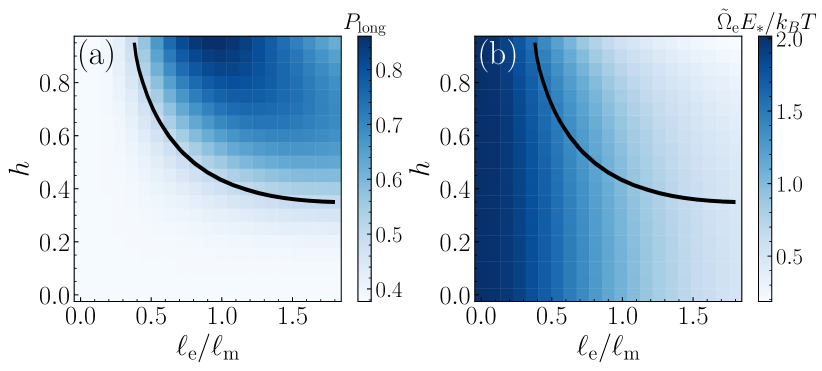
Figure 7: (a) Probability of finding the shape-switching molecule in the long state and (b) energy dissipation rate, versus the length ratio $\ell_{\textrm{e}}/\ell_{\textrm{m}}$ and the coupling strength $h$. The black line corresponds to $P_{\mathrm{long}}=0.5$. The noise strength is $k_{\rm B}T/\Delta=0.2$.

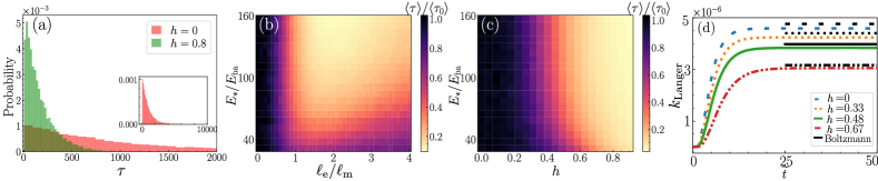
Figure 8: (a) Distribution of first passage times $\tau$ for $\ell_{\textrm{e}}/\ell_{\textrm{m}}=1.6$ in the absence (red) and presence (green) of dissipative coupling. (b,c) Mean first passage time $\langle\tau\rangle$, normalized by the mean first passage time in the uncoupled case where $\ell_{\textrm{e}}/\ell_{\textrm{m}}=0$, as a function of the length ratio $\ell_{\textrm{e}}/\ell_{\textrm{m}}$ and the energy ratio $E_{*}/E_{\mathrm{ba}}$ for fixed value of coupling strength $h=0.48$ (a), and as a function of the coupling strength $h$ and $E_{*}/E_{\mathrm{ba}}$ for fixed $\ell_{\textrm{e}}/\ell_{\textrm{m}}=1$ in (b). In (a–c), the noise strength is $k_{\rm B}T/\Delta=0.15$. (d) The rate at which the saddle point marked as the red diamond in Fig. 3 is crossed extracted numerically (coloured lines) compared to the Langer rate given by Eq. (16) (black horizontal lines), for $E_{\mathrm{ba}}/\Delta=0.8$ and $k_{\rm B}T/\Delta=0.08$.

The function of our model enzyme is most prominently dictated by the geometry of the enzyme-substrate complex, and can be optimized by following three simple golden rules: (i) the enzyme and the molecule should be attached at the smaller end of each; (ii) the conformational change of the enzyme must be comparable to or larger than the conformational change required of the molecule; (iii) the conformational change of the enzyme must be fast enough. These parameters can be experimentally tuned when designing an artificial enzyme, and should be experimentally accessible when investigating the function of biological enzymes. Interestingly, the effectiveness of the enzyme (as measured by successful catalytic action) and its energy dissipation do not follow a one-to-one relation (Fig. 7), leaving additional room for the optimization of not just the enzyme effectiveness but its energetic efficiency.

We were able to understand the emergence of a strong coupling between the thermodynamically favourable and unfavourable reactions to be a result of a global bifurcation in the deterministic dynamics of the system, of a similar nature to that causing synchronization and phase-locking among mechanically-coupled enzymes [35, 47]. Importantly, however, by adding thermodynamically-consistent fluctuations to the theory, we showed that the effect survives in the presence of noise, and we could calculate important quantities such as non-equilibrium steady states reflecting the departure from equilibrium thermodynamics in the reaction equilibrium, and first passage time distributions for the catalyzed reaction.

Our approach readily allows us to probe the energetic aspects of the non-equilibrium reaction [58], and in particular, the entropy production due to the coupling between the mechanical and the chemical degrees of freedom [59]. It can also be used to study evolutionary advantages of having mechanical control during the catalytic process via conformational changes, as opposed to simple utilization of the uncontrolled metal-based catalysis.

In conclusion, our model introduces new and important features to serve as a minimal model of a fuelled catalyst. This opens an avenue towards further progress in understanding and designing bio-inspired systems for artificial catalysis.

Appendix A Derivation of the phase-equations

We consider an enzyme and a molecule, both assumed to be dumbbell-shaped for simplicity. Upon binding, they are considered to be tightly linked together, thus forming a complex with three sub-units. The position vectors of the three sub-units are $\mathbf{r}_{\textrm{e}}$, $\mathbf{r}_{\textrm{b}}$ and $\mathbf{r}_{\textrm{m}}$ for the enzyme-only sub-unit, the bound enzyme-substrate sub-unit, and the molecule-only sub-unit, respectively. The lengths of the enzyme and molecule are therefore $\mathbf{L}_{\textrm{e}}=\mathbf{r}_{\textrm{b}}-\mathbf{r}_{\textrm{e}}=L_{\textrm{e}}\mathbf{\hat{n}}$ and $\mathbf{L}_{\textrm{m}}=\mathbf{r}_{\textrm{m}}-\mathbf{r}_{\textrm{b}}=L_{\textrm{m}}\mathbf{\hat{n}}$ where $\mathbf{\hat{n}}$ is the unit vector along the axis of the complex. The equations of motion for the sub-units are $\dot{r}_{\textrm{e}}=-\mu_{\textrm{e}}f_{\textrm{e}}$, $\dot{r}_{\textrm{b}}=\mu_{\textrm{b}}(f_{\textrm{e}}-f_{\textrm{m}})$ and $\dot{r}_{\textrm{m}}=\mu_{\textrm{m}}f_{\textrm{m}}$, where $f_{\textrm{e}}$ and $f_{\textrm{m}}$ are the internal mechanical forces (stresses) of the enzyme and molecule, respectively, which can be expressed as $f_{\textrm{e}}=-\partial_{L_{\textrm{e}}}U(L_{\textrm{e}},\phi_{\textrm{e}})$ and $f_{\textrm{m}}=-\partial_{L_{\textrm{m}}}V_{\textrm{m}}(L_{\textrm{m}})$. This implies that the equations of motion for the lengths are $\dot{L}_{\textrm{e}}=\mu_{1}f_{\textrm{e}}-\mu_{\textrm{b}}f_{\textrm{m}}$ and $\dot{L}_{\textrm{m}}=-\mu_{\textrm{b}}f_{\textrm{e}}+\mu_{2}f_{\textrm{m}}$, with the mobilities given as $\mu_{1}\equiv\mu_{\textrm{e}}+\mu_{\textrm{b}}$ and $\mu_{2}\equiv\mu_{\textrm{m}}+\mu_{\textrm{b}}$.

The governing dynamical equations for the two effective geometric degrees of freedom are therefore given by

$$\dot{L}_{\textrm{e}}=-\mu_{1}k[L_{\textrm{e}}-L(\phi_{\textrm{e}})]+\mu_{\textrm{b}}\partial_{L_{\textrm{m}}}V_{\textrm{m}}(L_{\textrm{m}}),$$ (17)

$$\dot{L}_{\textrm{m}}=\mu_{\textrm{b}}k[L_{\textrm{e}}-L(\phi_{\textrm{e}})]-\mu_{2}\partial_{L_{\textrm{m}}}V_{\textrm{m}}(L_{\textrm{m}}).$$ (18)

The dynamics of the internal enzyme phase is in turn given by

$$\dot{\phi}_{\textrm{e}} =\mu_{\phi}[-\partial_{\phi_{\textrm{e}}}U(L_{\textrm{e}},\phi_{\textrm{e}})],$$ (19)

$$=-\mu_{\phi}\left[-k(L_{\textrm{e}}-L(\phi_{\textrm{e}}))L^{\prime}(\phi_{\textrm{e}})+V^{\prime}_{\textrm{e}}(\phi_{\textrm{e}})\right],$$

with the prime representing a derivative with respect to $\phi_{\textrm{e}}$. We define $\delta L_{\textrm{e}}\equiv L_{\textrm{e}}-L(\phi_{\textrm{e}})$ such that $\dot{L}_{\textrm{e}}=\dot{\delta L_{\textrm{e}}}+L^{\prime}(\phi_{\textrm{e}})\dot{\phi}_{\textrm{e}}$. If the enzyme is relatively stiff with the timescale $(\mu_{1}k)^{-1}$ being much shorter than the timescale of changes in the internal phase, the enzyme length will quickly adapt to changes of the preferred length, and thus $\dot{\delta L_{\textrm{e}}}\approx 0$. From Eq. (17), this implies

$$L^{\prime}(\phi_{\textrm{e}})\dot{\phi}_{\textrm{e}}\approx-\mu_{1}k[L_{\textrm{e}}-L(\phi_{\textrm{e}})]+\mu_{\textrm{b}}\partial_{L_{\textrm{m}}}V(L_{\textrm{m}}),$$ (20)

which allows us to eliminate $k[L_{\textrm{e}}-L(\phi_{\textrm{e}})]$ between Eqs. (18) and (A), hence projecting the dynamics onto the slow manifold $(\phi_{\textrm{e}},L_{\textrm{m}})$. Finally, we reexpress $L_{\textrm{m}}$ in terms of the dimensionless reaction coordinate $\phi_{\textrm{m}}$ through $L_{\textrm{m}}=L_{\textrm{m}}^{(0)}+\ell_{\textrm{m}}\phi_{\textrm{m}}$. The resulting governing equations for $(\phi_{\textrm{e}},\phi_{\textrm{m}})$ then reduce to Eq. (1).

Appendix B Reverse switch reaction

One can observe that for the switch reaction our enzyme is equally capable of catalyzing a reverse reaction, i.e. from long to short conformational state, by choosing $\varepsilon<0$. Exploiting the symmetries of our dynamical equations, we find that a $\pi$ phase shift will be needed for $\phi_{\textrm{e}}$ in the conformation cycle (Eq. (8)), as in this case the enzyme will first contract and then expand during its conformational change. A phase portrait of the deterministic dynamics at strong coupling (beyond the global bifurcation) is shown in Fig. 9(a). This can be compared to the dynamics of the forward switch reaction in Fig. 3(d). Note that the bifurcation now happens near the upper saddle point, where the blue solid line represents the flow from the long state to the short state. An example of the NESS distributions for this reverse case is shown in Fig. 9(b), which may be compared to the case of the forward reaction in Fig. 5(b). It highlights how the action of the enzyme can favour the short state even if the long state is thermodynamically preferred.

Appendix C Simulations

To generate the phase portraits in Fig. 3 and the parameter scan in Fig. 4 from the deterministic equations (Eq. (1)), we used the built-in ode45 integrator of MATLAB, which uses a fourth order Runge-Kutta method [60]. A grid of $201\times 201$ for $-\pi<\phi_{\textrm{e}}<\pi$ and $-2<\phi_{\textrm{m}}<2$ was used to generate the initial conditions, and the equations were integrated for a total time of $\tilde{t}_{\rm tot}=120$.

For the numerical integration of the Fokker-Planck equation given by Eq. (5) we used a custom code written in Python [61]. The code uses a finite difference method with fourth-order accuracy for the spatial derivatives and fourth order Runge-Kutta method for the time integration. For the enzyme coordinate $\phi_{\textrm{e}}$ we considered the domain $0\leq\phi_{\textrm{e}}<2\pi$ with periodic boundary conditions. For the molecule coordinate $\phi_{\textrm{m}}$, we used Dirichlet boundary conditions in the domains $[-1.8,1.8],[-2.0,2.0],[-2.2,2.2]$ and noise strengths $k_{\rm B}T/\Delta=0.15,0.2,0.4$. To discretize the domains we used a rectangular shape domain such that the finite-difference increments satisfied $\Delta\phi_{\textrm{e}}\simeq\Delta\phi_{\textrm{m}}$ and thus the integrator would be more stable. For $k_{\rm B}T/\Delta=0.15,0.2,0.4$ the corresponding number of points $(N_{1},N_{2})$ per side were $(512,128),(400,128),(300,100)$, and the time step was $\Delta\tilde{t}=10^{-3},10^{-3},5\cdot 10^{-4}$.

For the numerical integration of the Langevin equations in Eq. (7), we used a custom code written in Julia [62]. The Euler-Maruyama method was used for the numerical integration. The time step used was $\Delta\tilde{t}=10^{-3}$.

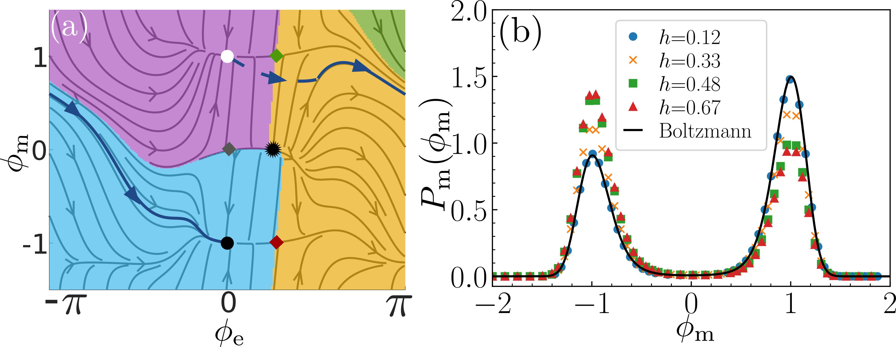
Figure 9: Reverse switch reaction. (a) Phase-portrait for $h=0.48$, $\ell_{\textrm{e}}/\ell_{\textrm{m}}=2.5$, and $\varepsilon/\Delta=-0.1$. The black solid line represents a deterministic trajectory. (b) Marginal distributions of the molecule reaction coordinate in steady-state, for various values of the coupling strength. (a) and (b) can be respectively compared to Fig. 3(d) and Fig. 5(b) for the forward reaction.

To check for consistency between the Langevin and Fokker-Planck approaches, long trajectories from the solution of the Langevin equations were binned and compared with the steady state distribution predicted by the Fokker-Planck equation. The two approaches exhibit good agreement, as depicted in Fig. 10 for the case of $h=0.67$ and $k_{\rm B}T/\Delta=0.2$.

Appendix D Steady state distribution for an uncoupled enzyme

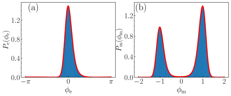
Figure 10: Comparison of the marginal distributions obtained from the Fokker-Planck equation (red solid line) at steady state and long simulations of the Langevin equations (histogram). (a) and (b) show the distribution of the enzyme and molecule reaction coordinates, respectively. The parameters for this example are $h=0.67$ and $k_{\rm B}T/\Delta=0.2$.

In the uncoupled case with $h=0$ or $\ell_{\textrm{e}}/\ell_{\textrm{m}}=0$, an exact expression for the steady state probability distribution for $\phi_{\textrm{e}}$ can be found. In the absence of coupling, the dynamics of $\phi_{\textrm{e}}$ at the steady state is determined by solving the following equation for a constant flux

$$J_{\mathrm{e}}=-M_{\mathrm{ee}}(\phi_{\textrm{e}})[V^{\prime}_{\textrm{e}}(\phi_{\textrm{e}})P_{\mathrm{e}}+k_{\rm B}T\partial_{\phi_{\textrm{e}}}P_{\mathrm{e}}].$$ (21)

Integrating this equation, we obtain

$$P_{\mathrm{e}}=e^{-V_{\textrm{e}}(\phi_{\textrm{e}})/k_{\rm B}T}\left[C-J_{\mathrm{e}}\int^{\phi_{\textrm{e}}}_{0}M_{\mathrm{ee}}^{-1}(x)e^{V_{\textrm{e}}(x)/k_{\rm B}T}dx\right],$$ (22)

where $C$ and $J_{\mathrm{e}}$ are constants of integration and are determined by the boundary conditions. Note that $M_{\mathrm{ee}}(\phi_{\textrm{e}})$ and $V_{\textrm{e}}^{\prime}(\phi_{\textrm{e}})$ are both $2\pi$-periodic. This implies that the probability distribution is also periodic, by following a similar derivation as in Ref. [53]. One finds that $C=\mathcal{N}I$ and $(1-e^{-2\pi F/k_{\rm B}T})\mathcal{N}=J_{\mathrm{e}}$, with $\mathcal{N}$ a normalization constant and

$$I=\int^{2\pi}_{0}dx\,M_{\mathrm{ee}}^{-1}(x)\,e^{V_{\textrm{e}}(x)/k_{\rm B}T}.$$ (23)

Hence, the full expression for the steady state marginal probability distribution for the enzyme reaction coordinate in the uncoupled case is

$$P_{\mathrm{e}}(\phi_{\textrm{e}})=\mathcal{N}\bigg{[}\int_{\phi_{\textrm{e}}}^{2\pi}dx\,M_{\mathrm{\textrm{e}\textrm{e}}}^{-1}(x)\exp\bigg{(}\frac{V_{\textrm{e}}(x)-V_{\textrm{e}}(\phi_{\textrm{e}})}{k_{\rm B}T}\bigg{)}$$

$$+\int^{\phi_{\textrm{e}}}_{0}dx\,M_{\textrm{e}\textrm{e}}^{-1}(x)\exp\bigg{(}\frac{V_{\textrm{e}}(x)-V_{\textrm{e}}(\phi_{\textrm{e}})-2\pi F}{k_{\rm B}T}\bigg{)}\bigg{]}.$$ (24)

The form of $V_{\textrm{e}}$ does not readily lend itself to further analytical progress, and we integrate Eq. (D) numerically to obtain the black lines in Fig. 5(a,c). In the particular case $E_{*}=0$, we find that $J_{\textrm{e}}=0$ and thus the enzyme coordinate is in thermodynamic equilibrium described by the Boltzmann weight $P_{\textrm{e}}(\phi_{\textrm{e}})\propto e^{-V_{\textrm{e}}(\phi_{\textrm{e}})/k_{\rm B}T}$.

Appendix E Langer rate

Starting from the Fokker-Planck equation, one derives the Langer rate through the enzyme saddle point to be [9, 56, 57]

$$k_{\rm Langer}=\frac{|\Lambda_{-}|}{2\pi}\frac{\sqrt{\lambda_{\mathrm{e}}^{(0)}\lambda_{\mathrm{m}}^{(0)}}}{\sqrt{|\lambda_{\mathrm{e}}|\lambda_{\mathrm{m}}}}\exp\bigg{(}{-\frac{E_{\mathrm{ba}}}{k_{\rm B}T}}\bigg{)},$$ (25)

where $\lambda_{\alpha}^{(0)}=V^{\prime\prime}_{\alpha}(\phi_{\alpha})|_{\rm min}$, and $\lambda_{\alpha}=V^{\prime\prime}_{\alpha}(\phi_{\alpha})|_{\rm saddle}$, namely, the corresponding values evaluated around the saddle point. The definitions imply that $\lambda_{\mathrm{m}}=\lambda_{\mathrm{m}}^{(0)}$, and thus, they cancel each other in Eq. (25). Finally, $\Lambda_{-}$ is the negative eigenvalue of the matrix $\lambda_{\alpha}M_{\alpha\beta}$ evaluated around the saddle point which is given by

$$\Lambda_{-}=\frac{1}{2}\bigg{(}M_{\textrm{e}\textrm{e}}\lambda_{\textrm{e}}+M_{\textrm{m}\textrm{m}}\lambda_{\textrm{m}}$$

$$\hskip 14.22636pt-\sqrt{(M_{\textrm{e}\textrm{e}}\lambda_{e}-M_{\textrm{m}\textrm{m}}\lambda_{\textrm{m}})^{2}+4M_{\textrm{e}\textrm{m}}^{2}\lambda_{\textrm{e}}\lambda_{\textrm{m}}}\bigg{)}.$$ (26)

References

- Borsley et al. [2024] S. Borsley, D. A. Leigh, and B. M. W. Roberts, Molecular Ratchets and Kinetic Asymmetry: Giving Chemistry Direction, Angew. Chem. Int. Ed. 63, e202400495 (2024).
- Michaelis and Menten [1913] L. Michaelis and M. L. Menten, Die kinetik der invertinwirkung, Biochemische Zeitschrift 49, 333 (1913).
- Johnson and Goody [2011] K. A. Johnson and R. S. Goody, The Original Michaelis Constant: Translation of the 1913 Michaelis–Menten Paper, Biochemistry 50, 8264 (2011).
- Qian [2007] H. Qian, Phosphorylation energy hypothesis: Open chemical systems and their biological functions, Annu. Rev. Phys. Chem. 58, 113 (2007).
- Lu [1998] H. P. Lu, Single-molecule enzymatic dynamics, Science 282, 1877–1882 (1998).
- English et al. [2005] B. P. English, W. Min, A. M. van Oijen, K. T. Lee, G. Luo, H. Sun, B. J. Cherayil, S. C. Kou, and X. S. Xie, Ever-fluctuating single enzyme molecules: Michaelis-Menten equation revisited, Nat. Chem. Biol. 2, 87–94 (2005).
- Kou et al. [2005] S. Kou, B. J. Cherayil, W. Min, B. P. English, and X. S. Xie, Single-molecule michaelis- menten equations, J. Phys. Chem. B 109, 19068 (2005).
- Kramers [1940] H. Kramers, Brownian motion in a field of force and the diffusion model of chemical reactions, Physica 7, 284 (1940).
- Hänggi et al. [1990] P. Hänggi, P. Talkner, and M. Borkovec, Reaction-rate theory: fifty years after Kramers, Rev. Mod. Phys. 62, 251 (1990).
- Karplus and McCammon [2002] M. Karplus and J. A. McCammon, Molecular dynamics simulations of biomolecules, Nat. Struct. Mol. Biol. 9, 646 (2002).
- Kutzner et al. [2019] C. Kutzner, S. Páll, M. Fechner, A. Esztermann, B. L. de Groot, and H. Grubmüller, More bang for your buck: Improved use of GPU nodes for GROMACS 2018, J. Comput. Chem. 40, 2418–2431 (2019).
- Lovelock et al. [2022] S. L. Lovelock, R. Crawshaw, S. Basler, C. Levy, D. Baker, D. Hilvert, and A. P. Green, The road to fully programmable protein catalysis, Nature 606, 49 (2022).
- Yeh et al. [2023] A. H.-W. Yeh, C. Norn, Y. Kipnis, D. Tischer, S. J. Pellock, D. Evans, P. Ma, G. R. Lee, J. Z. Zhang, I. Anishchenko, B. Coventry, L. Cao, J. Dauparas, S. Halabiya, M. DeWitt, L. Carter, K. N. Houk, and D. Baker, De novo design of luciferases using deep learning, Nature 614, 774–780 (2023).
- Dallago and Yang [2023] C. Dallago and K. K. Yang, Illuminating enzyme design using deep learning, Nat. Chem. 15, 749–750 (2023).
- Kathan et al. [2021] M. Kathan, S. Crespi, N. O. Thiel, D. L. Stares, D. Morsa, J. de Boer, G. Pacella, T. van den Enk, P. Kobauri, G. Portale, C. A. Schalley, and B. L. Feringa, A light-fuelled nanoratchet shifts a coupled chemical equilibrium, Nat. Nanotechnol. 17, 159–165 (2021).
- Corra et al. [2022] S. Corra, M. T. Bakić, J. Groppi, M. Baroncini, S. Silvi, E. Penocchio, M. Esposito, and A. Credi, Kinetic and energetic insights into the dissipative non-equilibrium operation of an autonomous light-powered supramolecular pump, Nat. Nanotechnol. 17, 746–751 (2022).
- Sorrenti et al. [2017] A. Sorrenti, J. Leira-Iglesias, A. Sato, and T. M. Hermans, Non-equilibrium steady states in supramolecular polymerization, Nat. Commun. 8 (2017).
- Pumm et al. [2022] A.-K. Pumm, W. Engelen, E. Kopperger, J. Isensee, M. Vogt, V. Kozina, M. Kube, M. N. Honemann, E. Bertosin, M. Langecker, R. Golestanian, F. C. Simmel, and H. Dietz, A DNA origami rotary ratchet motor, Nature 607, 492–498 (2022).
- Osat et al. [2024] S. Osat, J. Metson, M. Kardar, and R. Golestanian, Escaping kinetic traps using nonreciprocal interactions, Phys. Rev. Lett. 133, 028301 (2024).
- Osat and Golestanian [2023] S. Osat and R. Golestanian, Non-reciprocal multifarious self-organization, Nat. Nanotechnol. 18, 79 (2023).
- Ouazan-Reboul et al. [2023] V. Ouazan-Reboul, J. Agudo-Canalejo, and R. Golestanian, Self-organization of primitive metabolic cycles due to non-reciprocal interactions, Nat. Commun. 14, 4496 (2023).
- Glowacki et al. [2012] D. R. Glowacki, J. N. Harvey, and A. J. Mulholland, Taking ockham's razor to enzyme dynamics and catalysis, Nat. Chem. 4, 169 (2012).
- Callender and Dyer [2014] R. Callender and R. B. Dyer, The dynamical nature of enzymatic catalysis, Acc. Chem. Res. 48, 407 (2014).
- Jülicher et al. [1997] F. Jülicher, A. Ajdari, and J. Prost, Modeling molecular motors, Rev. Mod. Phys. 69, 1269 (1997).
- Kolomeisky and Fisher [2007] A. B. Kolomeisky and M. E. Fisher, Molecular motors: A theorist’s perspective, Annu. Rev. Phys. Chem. 58, 675–695 (2007).
- Mugnai et al. [2020] M. L. Mugnai, C. Hyeon, M. Hinczewski, and D. Thirumalai, Theoretical perspectives on biological machines, Rev. Mod. Phys. 92, 025001 (2020).
- Shi et al. [2022] X. Shi, A.-K. Pumm, J. Isensee, W. Zhao, D. Verschueren, A. Martin-Gonzalez, R. Golestanian, H. Dietz, and C. Dekker, Sustained unidirectional rotation of a self-organized DNA rotor on a nanopore, Nat. Phys. 18, 1105–1111 (2022).
- Shi et al. [2023] X. Shi, A.-K. Pumm, C. Maffeo, F. Kohler, E. Feigl, W. Zhao, D. Verschueren, R. Golestanian, A. Aksimentiev, H. Dietz, and C. Dekker, A DNA turbine powered by a transmembrane potential across a nanopore, Nat. Nanotechnol. (2023).
- Golestanian [2010] R. Golestanian, Synthetic mechanochemical molecular swimmer, Phys. Rev. Lett. 105, 018103 (2010).
- Golestanian and Ajdari [2008] R. Golestanian and A. Ajdari, Mechanical response of a small swimmer driven by conformational transitions, Phys. Rev. Lett. 100, 038101 (2008).
- Golestanian [2009] R. Golestanian, Anomalous diffusion of symmetric and asymmetric active colloids, Phys. Rev. Lett. 102, 188305 (2009).
- Golestanian [2015] R. Golestanian, Enhanced diffusion of enzymes that catalyze exothermic reactions, Phys. Rev. Lett. 115, 108102 (2015).
- Illien et al. [2017] P. Illien, T. Adeleke-Larodo, and R. Golestanian, Diffusion of an enzyme: The role of fluctuation-induced hydrodynamic coupling, EPL 119, 40002 (2017).
- Agudo-Canalejo et al. [2018] J. Agudo-Canalejo, T. Adeleke-Larodo, P. Illien, and R. Golestanian, Enhanced diffusion and chemotaxis at the nanoscale, Acc. Chem. Res. 51, 2365–2372 (2018).
- Agudo-Canalejo et al. [2021] J. Agudo-Canalejo, T. Adeleke-Larodo, P. Illien, and R. Golestanian, Synchronization and enhanced catalysis of mechanically coupled enzymes, Phys. Rev. Lett. 127, 208103 (2021).
- Zeravcic and Brenner [2014] Z. Zeravcic and M. P. Brenner, Self-replicating colloidal clusters, Proc. Natl. Acad. Sci. U.S.A. 111, 1748–1753 (2014).
- Zeravcic and Brenner [2017] Z. Zeravcic and M. P. Brenner, Spontaneous emergence of catalytic cycles with colloidal spheres, Proc. Natl. Acad. Sci. U.S.A. 114, 4342–4347 (2017).
- Zeravcic et al. [2017] Z. Zeravcic, V. N. Manoharan, and M. P. Brenner, Colloquium: Toward living matter with colloidal particles, Rev. Mod. Phys. 89, 031001 (2017).
- Rivoire [2020] O. Rivoire, Geometry and flexibility of optimal catalysts in a minimal elastic model, J. Phys. Chem. B 124, 807–813 (2020).
- Muñoz-Basagoiti et al. [2023] M. Muñoz-Basagoiti, O. Rivoire, and Z. Zeravcic, Computational design of a minimal catalyst using colloidal particles with programmable interactions, Soft Matter 19, 3933 (2023).
- Rivoire [2023] O. Rivoire, How flexibility can enhance catalysis, Phys. Rev. Lett. 131, 088401 (2023).
- Alberts et al. [1994] B. Alberts, D. Bray, J. Lewis, M. Raff, K. Roberts, J. D. Watson, et al., Molecular biology of the cell, Vol. 3 (Garland New York, 1994).
- Borsley et al. [2022] S. Borsley, D. A. Leigh, and B. M. W. Roberts, Chemical fuels for molecular machinery, Nat. Chem. 14, 728 (2022).
- Astumian and Bier [1996] R. Astumian and M. Bier, Mechanochemical coupling of the motion of molecular motors to ATP hydrolysis, Biophys. J. 70, 637 (1996).
- Eide et al. [2006] J. L. Eide, A. K. Chakraborty, and G. F. Oster, Simple models for extracting mechanical work from the ATP hydrolysis cycle, Biophys. J. 90, 4281 (2006).
- Chatzittofi et al. [2023a] M. Chatzittofi, R. Golestanian, and J. Agudo-Canalejo, Collective synchronization of dissipatively-coupled noise-activated processes, New J. Phys. 25, 093014 (2023a).
- Chatzittofi et al. [2023b] M. Chatzittofi, R. Golestanian, and J. Agudo-Canalejo, Topological phase locking in molecular oscillators, arXiv:2310.11788 (2023b).
- Lu et al. [2014] S. Lu, S. Li, and J. Zhang, Harnessing allostery: A novel approach to drug discovery, Med. Res. Rev. 34, 1242 (2014).
- Hehir et al. [2000] M. J. Hehir, J. E. Murphy, and E. R. Kantrowitz, Characterization of heterodimeric alkaline phosphatases from escherichia coli: An investigation of intragenic complementation, J. Mol. Biol. 304, 645 (2000).
- De Groot and Mazur [2013] S. R. De Groot and P. Mazur, Non-equilibrium thermodynamics (Courier Corporation, 2013).
- Kim and Karrila [2013] S. Kim and S. J. Karrila, Microhydrodynamics: principles and selected applications (Courier Corporation, 2013).
- Chatzittofi et al. [2024a] M. Chatzittofi, J. Agudo-Canalejo, and R. Golestanian, Nonlinear response theory of molecular machines, EPL 147, 21002 (2024a).
- Risken [1996] H. Risken, Fokker-Planck equation, in The Fokker-Planck Equation (Springer, 1996) pp. 63–95.
- Reimann et al. [2001] P. Reimann, C. Van den Broeck, H. Linke, P. Hänggi, J. M. Rubi, and A. Pérez-Madrid, Giant acceleration of free diffusion by use of tilted periodic potentials, Phys. Rev. Lett. 87, 010602 (2001).
- Reimann et al. [2002] P. Reimann, C. Van den Broeck, H. Linke, P. Hänggi, J. M. Rubi, and A. Pérez-Madrid, Diffusion in tilted periodic potentials: Enhancement, universality, and scaling, Phys. Rev. E 65, 031104 (2002).
- Langer [1968] J. S. Langer, Theory of nucleation rates, Phys. Rev. Lett. 21, 973 (1968).
- Langer [1969] J. Langer, Statistical theory of the decay of metastable states, Ann. Phys. 54, 258 (1969).
- Ragazzon and Prins [2018] G. Ragazzon and L. J. Prins, Energy consumption in chemical fuel-driven self-assembly, Nat. Nanotechnol. 13, 882–889 (2018).
- Chatzittofi et al. [2024b] M. Chatzittofi, J. Agudo-Canalejo, and R. Golestanian, Entropy production and thermodynamic inference for stochastic microswimmers, Phys. Rev. Res. 6, L022044 (2024b).
- Inc. [2023] T. M. Inc., Matlab version: 9.14.0 (r2023a) (2023).
- Van Rossum and Drake [2009] G. Van Rossum and F. L. Drake, Python 3 Reference Manual (CreateSpace, Scotts Valley, CA, 2009).
- Bezanson et al. [2012] J. Bezanson, S. Karpinski, V. B. Shah, and A. Edelman, Julia: A fast dynamic language for technical computing, arXiv:1209.5145 (2012).