Schwarz methods with PMLs for Helmholtz problems: fast convergence at high frequency

Abstract

We discuss parallel (additive) and sequential (multiplicative) variants of overlapping Schwarz methods for the Helmholtz equation in $\mathbb{R}^{d}$, with large real wavenumber and smooth variable wave speed. The radiation condition is approximated by a Cartesian perfectly-matched layer (PML). The domain-decomposition subdomains are overlapping hyperrectangles with Cartesian PMLs at their boundaries. In a recent paper (arXiv:2404.02156), the current authors proved (for both variants) that, after a specified number of iterations – depending on the behaviour of the geometric-optic rays – the error is smooth and smaller than any negative power of the wavenumber $k$. For the parallel method, the specified number of iterations is less than the maximum number of subdomains, counted with their multiplicity, that a geometric-optic ray can intersect. The theory, which is given at the continuous level and makes essential use of semi-classical analysis, assumes that the overlaps of the subdomains and the widths of the PMLs are all independent of the wavenumber. In this paper we extend the results of arXiv:2404.02156 by experimentally studying the behaviour of the methods in the practically important case when both the overlap and the PML width decrease as the wavenumber increases. We find that (at least for constant wavespeed), the methods remain robust to increasing $k$, even for miminal overlap, when the PML is one wavelength wide.

1 The Helmholtz problem

We consider the well-known Helmholtz equation:

$$-k^{-2}\Delta u-c^{-2}u=f\quad\text{in}\quad\mathbb{R}^{d},$$ (1)

with the Sommerfeld radiation condition: $r^{\frac{d-1}{2}}\left(\partial_{r}u-\mathrm{i}ku\right)\rightarrow 0,\ \text{as}\ r=|\mathbf{x}|\rightarrow\infty.$ Here $k\geq 1$ is the wave number, $c\in C^{\infty}(\mathbb{R}^{d})$ is the wavespeed and $f\in L^{2}(\mathbb{R}^{d})$ is the source. While the paper GaGoGrLaSp:24 treats the case of general $d$, in the interests of brevity we restrict here to $d=2$. The method for general $d$ is an obvious generalisation of the one presented here. We assume that both $f$ and $1-c$ are supported in a box $\Omega_{\rm int}:=(0,l)\times(0,d).$

We now restrict problem (1) to the domain $\Omega:=(-\kappa,l+\kappa)\times(-\kappa,d+\kappa)$, having added a standard Cartesian PML of thickness $\kappa$ to $\Omega_{\rm int}$. To do this, we choose a scaling function $f_{s}\in C^{\infty}(\mathbb{R})$ (with $s$ denoting “scaling”), satisfying

$$f_{s}(x)=f^{\prime}_{s}(x)=0\text{ for }x\leq 0\quad\text{and}\quad f^{\prime}_{s}(x)>0\text{ for }x>0,\ ,$$

together with $f_{s}(x)^{\prime\prime}=0\ \text{for}\ x\geq\kappa_{\rm lin}$ for some $\kappa_{\rm lin}<\kappa$. Using this, we define the horizontal and vertical scaling functions:

$$g_{1}(x_{1}):=\begin{cases}f_{s}(x_{1}-l)&\text{if }x_{1}\geq l\\ 0&\text{if }x_{1}\in(0,l)\\ {-}f_{s}(-x_{1})&\text{if }x_{1}\leq 0\end{cases},\hskip 8.5359ptg_{2}(x_{2}):=\begin{cases}f_{s}(x_{2}-d)&\text{if }x_{2}\geq d\\ 0&\text{if }x_{2}\in(0,d)\\ {-}f_{s}(-x_{2})&\text{if }x_{2}\leq 0\end{cases},$$

and the scaled operator

$$\Delta_{s}:=\Big{(}\gamma_{1}(x_{1})^{-1}\partial_{x_{1}}\Big{)}^{2}+\Big{(}\gamma_{2}(x_{2})^{-1}\partial_{x_{2}}\Big{)}^{2},$$ (2)

where $\gamma_{m}:=1+ig_{m}^{\prime}$, $m=1,2$. The PML approximation to (1) then reads as:

$$P_{s}\,u\ :=\ (-k^{-2}\Delta_{s}-c^{-2})\,u =f\quad\text{on }\quad\Omega,$$ (3)

$$\text{subject to}\quad u =0\quad\text{on }\quad\partial\Omega.$$

2 The overlapping Schwarz methods with local PMLs

We consider both parallel and sequential overlapping Schwarz methods for (3), using PML as a subdomain boundary condition. Such a strategy was first proposed (without theory) in To:98 , and has received much recent interest both in the overlapping and non-overlapping cases – for reviews see GaGoGrLaSp:24 and GaZh:22 . Recent work on the overlapping case includes LeJu:19 and BoBoDoTo:22 . Our paper GaGoGrLaSp:24 provides the first wavenunber-explicit theory, both for the overlapping case, and for any domain decomposition method for Helmholtz problems with a non-trivial scatterer.

We cover $\Omega_{\rm int}$ by $N$ overlapping sub-rectangles: $\Omega_{{\rm int},j}:=(a^{j},b^{j})\times(c^{j},d^{j}),\ j=1,\ldots,N$, and we let $\delta>0$ denote the minimum overlap parameter, as defined for example in (ToWi:05, , Assumption 3.1). Each $\Omega_{\rm int,j}$ is then extended to a larger subdomain $\Omega_{j}$ by adding a PML of width $\kappa$ along each edge, analogous to the extension of $\Omega_{\rm int}$ to $\Omega$. (The PML width on interior edges could also be different from $\kappa$ - see GaGoGrLaSp:24 .)

An example is the checkerboard decomposition, where the $\Omega_{{\rm int},j}$ are constructed by starting with an $N_{1}\times N_{2}$ tensor product rectangular (non-overlapping) decomposition of $\Omega_{\rm int}$ and then extending the internal boundary of each sub-rectangle outward, subject to the constraint that each extended sub-rectangle only overlaps its nearest neighbours. Then, Cartesian PMLs are added to $\Omega_{\rm int}$ and $\Omega_{{\rm int},j}$ as above. A checkerboard with either $N_{1}=1$ or $N_{2}=1$ is called a strip decompositon. In any case $N:=N_{1}N_{2}$ is the number of subdomains.

We now define subproblems on $\Omega_{j}$, $j=1,\ldots,N$. The local scaling functions are

$$g_{1,j}(x_{1}):=\begin{cases}f_{s}(x_{1}-{b}_{j})&\text{if }x_{1}\geq{b}_{j}\\ 0&\text{if }x_{1}\in({a}_{j},{b}_{j})\\ {-}f_{s}({a}_{j}-x_{1})&\text{if }x_{1}\leq{a}_{j}\end{cases},\hskip 8.5359ptg_{2,j}(x_{2}):=\begin{cases}f_{s}(x_{2}-{d}_{j})&\text{if }x_{2}\geq{d}_{j}\\ 0&\text{if }x_{2}\in({c}_{j},{d}_{j})\\ {-}f_{s}({c}_{j}-x_{2})&\text{if }x_{2}\leq{c}_{j}.\end{cases},$$

Then the local scaled Laplace operators (analogous to (2)) are

$$\Delta_{s,j}:=\Big{(}\gamma_{1,j}(x_{1})^{-1}\partial_{x_{1}}\Big{)}^{2}+\Big{(}\gamma_{2,j}(x_{2})^{-1}\partial_{x_{2}}\Big{)}^{2},$$ (4)

where $\gamma_{m,j}=1+ig_{m,j}^{\prime},m=1,2$ and the local scaled Helmholtz operator is

$$P_{s,j}:=-k^{-2}\Delta_{s,j}-c^{-2}.$$ (5)

To knit local solutions together, we introduce a partition of unity on $\mathbb{R}^{2}$, denoted $\{\chi_{j}\}_{j=1}^{N}$, such that $\sum_{j}\chi_{j}\equiv 1\ \text{on}\ \mathbb{R}^{2}$, and, in addition,

$$\mathrm{supp}\chi_{j}\cap\Omega\subseteq\{x\in\Omega_{j}:g_{\ell,j}(x_{\ell})=g_{\ell}(x_{\ell}),\ \ell=1,2\}.$$ (6)

Condition (6) implies that $\mathrm{supp}\chi_{\ell}\subseteq\Omega_{{\rm int},j}$ if $\Omega_{{\rm int},j}$ is an interior subdomain of $\Omega_{\rm int}$ but $\mathrm{supp}\chi_{\ell}$ is extended into the PML of $\Omega_{\rm int}$ otherwise. The algorithms are then as follows.

The additive (parallel) Schwarz method.  Given an initial guess $u_{+}^{0}\in H^{1}_{0}(\Omega)$, we obtain the iterates $u_{+}^{n}:n=1,2,\ldots$ by solving (variationally) the local problem:

$$P_{s,j}\mathfrak{c}_{j}^{n}=(f-P_{s}u_{+}^{n})|_{\Omega_{j}}\quad\text{on}\quad\Omega_{j}$$ (7)

for the corrector $\mathfrak{c}_{j}^{n}\in H^{1}_{0}(\Omega_{j})$, and then setting

$$u_{+}^{n+1}=u_{+}^{n}+\sum_{j=1}^{N}\chi_{j}\mathfrak{c}_{j}^{n}.$$ (8)

If we introduce $u_{j}^{n+1}:=u_{+}^{n}|_{\Omega_{j}}+\mathfrak{c}_{j}^{n}$, then this can also be written:

$$P_{s,j}u_{j}^{n+1} =P_{s,j}(u_{+}^{n}|_{\Omega_{j}})-(P_{s}u_{+}^{n})|_{\Omega_{j}}+f|_{\Omega_{j}}\ \text{on}\ \Omega_{j},\quad\text{with}\ u_{j}^{n+1} =u_{+}^{n}\quad\text{on}\ \partial\Omega_{j},$$

and then $u_{+}^{n+1}:=\sum_{j=1}^{N}\chi_{j}u_{j}^{n+1}$. In this case, all the local contributions $u_{j}^{n+1}:j=1,\ldots,N$ are computed independently in parallel, before $u_{+}^{n+1}$ is finally assembled. The sequential version is a simple variant of this.

The multiplicative (sequential) Schwarz method.   Given an initial guess $u_{\times}^{0}\in H^{1}_{0}(\Omega)$, let $u^{0}_{j}:=u_{\times}^{0}|_{\Omega_{j}}.$ Then, for $n=0,1,\ldots$, do the following:

1. (Forward sweeping) For $j=1,\ldots,N$,

   $$u_{j,n}^{\rightarrow}:=\sum_{\ell<j}\chi_{\ell}u_{\ell}^{2n+1}+\sum_{\ell\geq j}\chi_{\ell}u_{\ell}^{2n}$$

   and then compute $u_{j}^{2n+1}\in H^{1}(\Omega_{j})$ as the solution to

   $$P_{s,j}u_{j}^{2n+1} =P_{s,j}(u_{j,n}^{\rightarrow}|_{\Omega_{j}})-(P_{s}u_{j,n}^{\rightarrow})|_{\Omega_{j}}+f|_{\Omega_{j}}\quad\text{on}\quad\Omega_{j},$$

   $$\text{subject to}\quad u_{j}^{2n+1} =u_{j,n}^{\rightarrow}\quad\text{on}\quad\partial\Omega_{j},$$

   Then set

   $$u_{\times}^{2n+1}:=\sum_{\ell=1}^{N}\chi_{\ell}u_{\ell}^{2n+1}.$$

2. (Backward sweeping) For $j=N,\ldots,1$, introduce

   $$u_{j,n}^{\leftarrow}:=\sum_{\ell\leq j}\chi_{\ell}u_{\ell}^{2n+1}+\sum_{j<\ell}\chi_{\ell}u_{\ell}^{2n+2}\,\in H^{1}_{0}(\Omega).$$

   Then compute $u_{j}^{2n+2}\in H^{1}(\Omega_{j})$ as the solution to

   $$P_{s,j}u_{j}^{2n+2} =P_{s,j}(u_{j,n}^{\leftarrow}|_{\Omega_{j}})-(P_{s}u_{j,n}^{\leftarrow})|_{\Omega_{j}}+f|_{\Omega_{j}}\quad\text{on}\quad\Omega_{j},$$

   $$\text{subject to}\quad u_{j}^{2n+2} =u_{j,n}^{\leftarrow}\quad\text{on}\quad\partial\Omega_{j},$$

   and then set

   $$u_{\times}^{2n+2}:=u^{\leftarrow}_{N+1,n}=\sum_{\ell=1}^{N}\chi_{\ell}u_{\ell}^{2n+2}.$$

Remark 1

General sequential methods for any dimensional checkerboard decompositions can be found in (GaGoGrLaSp:24, , Section 1.4.6). These methods perform multiple sweepings with different orders of the subdomains. Specifically, we construct exhaustive (see (GaGoGrLaSp:24, , Definition 7.2)) sweeping methods such that, for each geometric-optic ray, there are at least two sweeps ordering the subdomains intersected along the ray in both forward and backward directions.

3 Theoretical results

Suppose the POU $\{\chi_{j}\}$ is $C^{\infty}$ Let $\{u^{n}_{*}\}_{n=0}^{\infty}$ be any sequence of iterates for the additive ($*=+$) or multiplicative ($*=\times$) Schwarz algorithm above. Then (GaGoGrLaSp:24, , Theorems 1.1-1.4 and 1.6) give conditions that, for any $M>0$ and integer $s\geq 1$, guarantee the existence of ${\mathcal{N}}\in\mathbb{N}$ and $C>0$ (both independent of $f$) such that

$$\|u-u^{\mathcal{N}}_{*}\|_{H_{k}^{s}(\Omega)}\leq Ck^{-M}\|u-u^{0}_{*}\|_{H_{k}^{1}(\Omega)}.$$ (9)

(Here the norm is defined by $\left\|v\right\|^{2}_{H^{s}_{k}(\Omega)}:=\sum_{|\alpha|\leq s}\left\|(k^{-1}\partial)^{\alpha}v\right\|^{2}_{L^{2}(\Omega)},\ \text{for}\ s\geq 1.$)

In particular, (9) implies that the fixed-point iterations converge exponentially quickly in the number of iterations for sufficiently-large $k$ and the rate of exponential convergence increases with $k$.

The case of no scatterer ($c\equiv 1$) is dealt with in (GaGoGrLaSp:24, , Theorems 1.1-1.4). In that case, for a strip DD with $N$ subdomains, ${\mathcal{N}}=N$ for the parallel algorithm while ${\mathcal{N}}=2$ for the sequential algorithm (one forward and backward sweep). For a 2D checkerboard with $N_{1}\geq 2$ and $N_{2}\geq 2$, we have ${\mathcal{N}}=N_{1}+N_{2}-1$ in the parallel case and ${\mathcal{N}}=4$ in the sequential case (although the ordering of sweeps has to be carefully chosen). The case of variable (but non-trapping) $c$ and general rectangular DD is dealt with in (GaGoGrLaSp:24, , Theorems 1.6), where ${\mathcal{N}}$ is defined as the maximum number of subdomains, counted with their multiplicity, that a geometric-optic ray can intersect.

These results are valid on fixed domains for sufficiently-large $k$, i.e., the PML widths and DD overlaps are arbitrary, but assumed independent of $k$. Obtaining results that are also explicit in these geometric parameters of the decomposition will require more technical arguments than those used in GaGoGrLaSp:24 . In this paper we investigate this issue experimentally.

4 Discretisation and numerical results

Discretisation.  Equation (3), involving the scaled operator $P_{s}$, is recast in variation form, multiplying by a test function $v\in H^{1}_{0}(\Omega)$ and integrating by parts to obtain

$$a(u,v):=\int_{\Omega}k^{-2}\big{(}(D\nabla u)\cdot\nabla\overline{v}-(\beta\cdot\nabla u)\overline{v}\big{)}-c^{-2}u\overline{v}=\langle f,v\rangle_{L^{2}(\Omega)}.$$ (10)

$$\text{where}\quad D:=\mathrm{diag}\left(\gamma_{1}^{-2}(x_{1}),\gamma_{2}^{-2}(x_{2})\right)\ \text{ and }\ \beta:=\left(\gamma_{1}^{\prime}(x_{1})\gamma_{1}^{-3}(x_{1})\,,\,\gamma_{2}^{\prime}(x_{2})\gamma_{2}^{-3}(x_{2})\right)^{T}.$$

The variational form of equations involving the local operator $P_{s,j}$ (such as (7)) yield an analogous local sesquilinear form $a_{j}$ defined on $H^{1}_{0}(\Omega_{j})^{2}$.

Let $\{\mathcal{T}_{h}\}$ be a shape-regular conforming sequence of meshes for $\Omega$ which resolve the boundaries of $\Omega$, $\Omega_{\rm int}$, $\Omega_{\rm int,j}$, and $\Omega_{j}$, for all $j$. Let $V_{h}$ be the space of continuous piecewise-polynomials of degree $\leq p$ on $\mathcal{T}_{h}$ which vanish on $\partial\Omega$. The finite element discretisation of (10) leads to the linear algebraic system $\mathsf{Au=f}$, with $\mathsf{u}$ denoting the nodal vector of the finite element solution to be found.

Then, with $V_{h,j}=\{v_{h}|_{\Omega_{j}}:v_{h}\in V_{h}\}\cap H^{1}_{0}(\Omega_{j})$, the discrete version of the additive algorithm reads as follows. Given an iterate $u^{n}_{+,h}\in V_{h}$, we compute a corrector $\mathfrak{c}_{h,j}^{n}\in V_{h,j}$ by solving the discrete version of (7):

$$a_{j}\big{(}\mathfrak{c}_{h,j}^{n},v_{h,j}\big{)}=\big{\langle}f,\mathcal{R}^{T}_{h,j}v_{h,j}\big{\rangle}-a\big{(}u^{n}_{h,j},\mathcal{R}^{T}_{h,j}v_{h,j}\big{)}\quad\text{ for all }v_{h,j}\in V_{h,j}.$$

where $\mathcal{R}_{h,j}^{\top}$ denotes extension by zero from $V_{h,j}$ to $V_{h}$. The next iterate $u_{+,h}^{n+1}$ is obtained by the discrete analogue of (8).

With $\mathsf{A}_{j}$ denoting the finite element stiffness matrix corresponding to $a_{j}$, and $\mathsf{u}_{+}^{n}$ denoting the nodal vector of the $n$th iterate, this can be easily seen to correspond to the preconditioned Richardson iteration (see (GaGoGrLaSp:24, , §8)):

$$\mathsf{u}^{n+1}_{+}:=\mathsf{u}^{n}_{+}+\mathsf{B}^{-1}(f-\mathsf{A}\mathsf{u}^{n}_{+})\quad\text{ with }\quad\mathsf{B}^{-1}:=\sum_{j}\widetilde{\mathsf{R}}_{j}^{\top}\mathsf{A}_{j}^{-1}\mathsf{R}_{j},$$

where $\mathsf{R}_{j}$ denotes the restriction of a nodal vector on $\Omega$ to its nodes on $\Omega_{j}$, and $\widetilde{\mathsf{R}}_{j}^{\top}$ denotes the extension by zero of a nodal vector on $\Omega_{j}$, after multiplication by nodal values of $\chi_{j}$. Thus the additive algorithm is a familiar restricted additive Schwarz method where the subdomain problems have PML boundary conditions.

Numerical Experiment.  In this experiment, we explore how the overlap size $\delta$ and the definition of the PML affect the performance of the methods. For discretization, we used finite elements of polynomial order $2$, with $h\sim k^{-1.25}$ (to control the pollution error). In the tests in GaGoGrLaSp:24 (chosen to illustrate the theory), we had set $\delta=\kappa=1/40$, fixed independently of $k$. In this case the number of freedoms in the overlaps and the PMLs increases significantly as $k$ increases, implying a heavy communication load at high-frequency. Here we investigate smaller PML thickness $\kappa$ and smaller overlap $\delta$, thus increasing the practicality of the method. The PML scaling function is $f_{\rm PML}(x)=\frac{a}{3}x^{3}$.

We tested two possible choices of $\kappa$ and $a$. In the first setting we chose $\kappa=\lambda:=\frac{2\pi}{k}$ (i.e., the PML is one wavelength wide) and we compared different choices of $a\in\{5\times 10^{3},\,10^{4},\,30k,\,0.3k^{2}\}$. In the second setting we chose $\kappa\in\{3h,5h\}$ and $a=k^{2.5}$, (thus ensuring that the PML scaling functions have the same maximal modulus $\mathcal{O}(1)$ in the PML regions). The second setting turned out not to be $k$-robust, while the first was found to perform better when $a$ was increasing with respect to $k$. Due to the page limit, we only present the results for $\kappa=\lambda$ and $a=30k$ and for overlap $\delta\in\{\frac{1}{80},2h,h\}$; when $\delta=h$ the overlap has only two layers of elements.

Regarding the POU, for a strip DD we start from functions $\tilde{\chi}_{j}$ supported on $\Omega_{{\rm int},j}$, which take value $1$ in the non-overlapping region and decrease linearly to $0$ towards the internal boundary of $\Omega_{{\rm int},j}$. Then the PoU is obtained by normalizing, i.e., $\chi_{j}=\frac{\tilde{\chi}_{j}}{\sum_{j}\tilde{\chi}_{j}}.$ For the checkerboard DD, we used the Cartesian product $\tilde{\chi}_{i}(x)\tilde{\chi}_{j}(y)$ to generate local functions on $\Omega_{{\rm int},j}$ and then normalized them to obtain $\chi_{j}$. The POU used here is not as smooth as is required in the theoretical analysis GaGoGrLaSp:24 . In fact, in the experiments in GaGoGrLaSp:24 we used a smooth PoU and each $\chi_{j}$ was supported in a proper subset of $\Omega_{{\rm int},j}$, bounded away from $\partial\Omega_{{\rm int},j}$.

Table 1 lists the iteration counts for the algorithms to attain 1e-6 reduction of the relative residual. Here “RAS-PML” and “RMS-PML” denote respectively the additive and multiplicative algorithms, each tested on strip and checkerboard DDs. For the RMS-PML and checkerboard DD, we use the exhaustive sweeping method that contains 4 sweeps per iteration (see (GaGoGrLaSp:24, , Figure 1.2)). We observe:

*  The performance is hardly degraded when the overlap is reduced from fixed ($\delta=1/80$) to minimal ($\delta=h$). When $\delta=1/80$, the overlap contains $4,7,10,13,16,19$ layers of elements for $k=100,150,200,250,300,350$. The results show that this communication cost can be removed while hardly affecting the convergence.

*  With $\kappa=\lambda$, the iteration counts are not decreasing as fast with increasing $k$ as when we used fixed PML width. (See the experiments in GaGoGrLaSp:24 illustrating (9).) However convergence rates remain bounded for the range of $k$ tested and in the checkerboard case for RAS-PML, the convergence rate decreases as the wave number increases; see Figure 1.

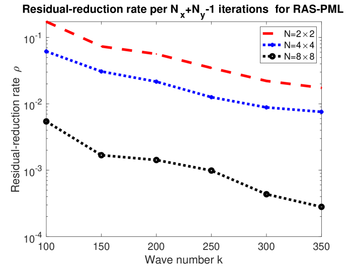
(a) checkerboard, RAS-PML: $\rho=\frac{\|\mathsf{A(u-u^{N_{x}+N_{y}-1})}\|_{\ell^{2}}}{\|\mathsf{A(u-u^{0})}\|_{\ell^{2}}}$

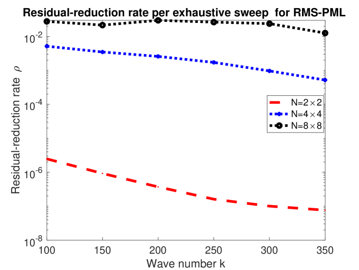
(b) checkerboard, RMS-PML: $\rho=\frac{\|\mathsf{A(u-u^{4})}\|_{\ell^{2}}}{\|\mathsf{A(u-u^{0})}\|_{\ell^{2}}}$

Figure 1: RAS-PML on Checkerboard: The rate of reduction of the residual against $k$

N	2			4			8
k\$\delta$	$\frac{1}{80}$	2h	h	$\frac{1}{80}$	2h	h	$\frac{1}{80}$	2h	h
100	3(3)	4(4)	4(4)	7(7)	7(7)	7(7)	15(15)	15(15)	15(15)
150	3(3)	3(3)	3(3)	7(7)	7(7)	7(7)	15(15)	15(15)	15(15)
200	3(3)	4(3)	4(3)	7(7)	7(7)	7(7)	12(12)	15(15)	15(15)
250	4(4)	4(4)	4(4)	6(6)	7(7)	7(7)	11(11)	15(15)	15(15)
300	4(4)	5(5)	5(5)	7(7)	7(7)	7(7)	15(15)	15(15)	15(15)
350	4(4)	5(5)	5(5)	6(6)	7(7)	7(7)	11(11)	14(14)	15(15)

(a) RAS-PML on strip DD

N	$2\times 2$			$4\times 4$			$8\times 8$
k\$\delta$	$\frac{1}{80}$	2h	h	$\frac{1}{80}$	2h	h	$\frac{1}{80}$	2h	h
100	8(6)	9(6)	9(7)	18(16)	19(18)	20(19)	33(27)	40(32)	47(36)
150	8(6)	8(6)	8(7)	16(15)	18(18)	20(18)	32(27)	42(37)	48(40)
200	7(6)	8(6)	8(7)	15(14)	18(17)	19(18)	30(28)	48(37)	56(40)
250	7(6)	8(6)	8(6)	14(13)	19(16)	20(17)	29(27)	42(37)	45(39)
300	6(6)	8(6)	8(7)	13(13)	18(16)	18(17)	28(27)	44(37)	47(39)
350	6(6)	7(6)	7(7)	13(13)	17(16)	18(16)	28(26)	45(37)	48(39)

(b) RAS-PML on checkerboard DD

N 2 4 8 k\$\delta$ $\frac{1}{80}$ 2h h $\frac{1}{80}$ 2h h $\frac{1}{80}$ 2h h 100 2 2 2 2 2 2 2 2 2 150 2 2 2 2 2 2 2 2 2 200 2 2 2 2 2 2 2 2 2 250 2 2 2 2 2 2 2 2 2 300 2 3 3 2 3 3 2 3 3 350 2 3 3 2 3 3 2 3 3

N $2\times 2$ $4\times 4$ $8\times 8$ k\$\delta$ $\frac{1}{80}$ 2h h $\frac{1}{80}$ 2h h $\frac{1}{80}$ 2h h 100 2 2 2 4 4 4 5 5 6 150 2 2 2 3 4 4 4 5 6 200 2 2 2 3 4 4 4 5 6 250 2 2 2 3 4 4 4 5 6 300 2 2 2 3 3 4 4 5 5 350 2 2 2 3 3 3 3 5 5

(c) RMS-PML:  Left: strip DD, Right checkerboard DD.

Table 1: Iteration counts (relative residual tol = $10^{-6}$) with $f_{\rm PML}(x):=\frac{a}{3}x^{3}$,  $a=30k$. Note that $\frac{1}{80h}=4,7,10,13,16,19$ for $k=100,150,200,250,300,350$

Acknowledgement JG was supported by EPSRC grant EP/V001760/1. SG was supported by the National Natural Science Foundation of China (Grant number 12201535) and the Guangdong Basic and Applied Basic Research Foundation (Grant number 2023A1515011651). DL was supported by INSMI (CNRS) through a PEPS JCJC grant 2023. EAS was supported by EPSRC grant EP/R005591/1. IGG was supported for several collaborative visits by CUHK Shenzhen.

References

• (1) N. Bootland, S. Borzooei, V. Dolean, and P.-H. Tournier. Numerical assessment of PML transmission conditions in a domain decomposition method for the Helmholtz equation. In International Conference on Domain Decomposition Methods, pages 445–453. Springer, 2022.
• (2) J. Galkowski, S. Gong, I. G. Graham, D. Lafontaine, E. A. Spence, Convergence of overlapping domain decomposition methods with PML transmission conditions applied to nontrapping Helmholtz problems, arXiv:2404.02156, April 2024.
• (3) A. Toselli. Overlapping method with perfectly matched layers for the solution of the Helmholtz equation. In Proceedings of the 11th International Conference on Domain Decomposition Methods, pages 551–557, 1998. http://www.ddm.org/DD11/DD11proc.pdf.
• (4) A. Toselli and O.B. Widlund, Domain Dercompositions Methods – Algorithms and Theory, Springer, Berlin, 2005.
• (5) W. Leng and L. Ju. An additive overlapping domain decomposition method for the Helmholtz equation. SIAM Journal on Scientific Computing, 41(2):A1252–A1277, 2019.
• (6) M. J. Gander and H. Zhang. Schwarz methods by domain truncation. Acta Numerica, 2022.
• (7) S. Gong, M.J. Gander, I. G. Graham, D. Lafontaine, and E. A Spence. Convergence of overlapping domain decomposition methods for the Helmholtz equation. Numerische Mathematik, 152(2):259–306, 2022.