Seeking the Sufficiency and Necessity Causal Features in Multimodal Representation Learning

Abstract

Learning representations with a high Probability of Necessary and Sufficient Causes (PNS) has been shown to enhance deep learning models’ ability. This task involves identifying causal features that are both sufficient (guaranteeing the outcome) and necessary (without which the outcome cannot occur). However, current research predominantly focuses on unimodal data, and extending PNS learning to multimodal settings presents significant challenges. The challenges arise as the conditions for PNS identifiability—Exogeneity and Monotonicity—need to be reconsidered in a multimodal context, where sufficient and necessary causal features are distributed across different modalities. To address this, we first propose conceptualizing multimodal representations as comprising modality-invariant and modality-specific components. We then analyze PNS identifiability for each component, while ensuring non-trivial PNS estimation. Finally, we formulate tractable optimization objectives that enable multimodal models to learn high-PNS representations, thereby enhancing their predictive performance. Experiments demonstrate the effectiveness of our method on both synthetic and real-world data.

Introduction

Probability of Necessary and Sufficient Causes (PNS) measures the likelihood of a feature set being both necessary and sufficient for an outcome (Pearl 2009). Recently, PNS estimation has been successfully extended to guide representation learning in unimodal data, improving models’ ability to capture the underlying causal information from data (Yang et al. 2024; Wang and Jordan 2021; Chen et al. 2024; Cai et al. 2024). However, applying PNS estimation to multimodal context remains underexplored, even though it is increasingly important to learn meaningful representations from diverse modalities (Xu et al. 2024; Liu et al. 2024b; Liang et al. 2024a, b; Swamy et al. 2024; Tang et al. 2024; Dong et al. 2023). The challenges in this application arise from the difficulty in satisfying two conditions for PNS identifiability: Exogeneity and Monotonicity.

Exogeneity requires causal features to be identifiable from observational data without influence from unmeasured confounders. In multimodal scenarios, inter-modal interactions can compromise this condition. Additionally, treating multimodal data as unimodal can violate Exogeneity, since the features may become unidentifiable without strong assumptions or additional supervision (Yang et al. 2024; Wang and Jordan 2021; Locatello et al. 2019; Liu et al. 2021).

Monotonicity, on the other hand, implies that causal features monotonically influence outcome prediction. However, the intricate interactions in multimodal data could result in non-monotonic relationships. The high-dimensional, continuous nature of such data further complicates the assessment of consistent directional effects across modalities.

To address the challenges and extend PNS estimation into multimodal scenarios, we propose viewing multimodal hidden features as consisting of two components: modality-invariant contains shared information across different modalities, and modality-specific retains the unique characteristics of each modality (Zhang et al. 2019; Ramachandram and Taylor 2017; Guo, Wang, and Wang 2019; Gao et al. 2020; Li, Wang, and Cui 2023). Then, we derive how to satisfy PNS identifiability for them and introduce additional contraints for non-trivial PNS estimation. Using these insights, we design objective functions for learning high-PNS multimodal representations.

Our contributions are: First, we introduce the concept of PNS in multimodal representation learning and analyze its associated challenges. Second, we propose considering multimodal features as two components and derive PNS estimation tailored for these components. Finally, we propose optimization objectives based on these findings to enhance multimodal representation learning. Experimental results on both synthetic and real-world datasets demonstrate the effectiveness of our method.

Related Works

Causal representation learning. Causal representation learning aims to identify underlying causal information from observational data (Schölkopf et al. 2021), which is crucial for enhancing the trustworthiness of machine learning tasks, particularly in explanation, generalization, and robustness (Arjovsky et al. 2019; Hu et al. 2018; Ahuja et al. 2020; Gamella and Heinze-Deml 2020). It mainly encompasses causal relationship discovery and causal feature learning. Causal relationship discovery (Peters et al. 2014; Zheng et al. 2018; Huang et al. 2020; Zhu, Ng, and Chen 2019) focuses on uncovering the causal structure among variables. On the other hand, causal feature learning (Zhang et al. 2020; Chen et al. 2022; Louizos et al. 2017; Yang et al. 2021; Lu et al. 2021) aims to extract features that have a causal relationship with the target outcome. To extract meaningful features, the PNS (Pearl 2009), proposed in Pearl’s framework, serves as a powerful tool. By capturing causal features with high PNS values, learned representations can improve the stability and interpretability of deep learning models. Recognizing this potential, recent studies have explored PNS applications in causal feature learning, including learning invariant representations (Yang et al. 2024), identifying causally relevant features (Cai et al. 2024), and formulating efficient low-dimensional representations (Wang and Jordan 2021). However, they primarily focus on unimodal data, leaving the challenges of multimodal data unaddressed.

Multimodal learning. Multimodal learning focuses on capturing meaningful representations from multiple modalities (Islam et al. 2023; Zhang, Kong, and Zhou 2023; Tran et al. 2024; Liu et al. 2024a). To achieve this, various methods have been developed to disentangle multimodal representations into modality-invariant and modality-specific parts (Shi et al. 2019; Tsai et al. 2018; Mai, Hu, and Xing 2020; Wang et al. 2017; Li, Wang, and Cui 2023).

Our study bridges these two areas to address the challenges of applying PNS estimation in multimodality. We propose viewing multimodal representations as two components, derive how to compute non-trival PNS for them, and use the theoretical finding to design objective functions for learning high-PNS multimodal representations.

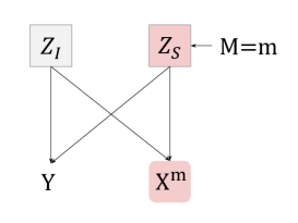
Figure 1: Causal graph

Preliminaries

Problem Setup

Let $m\in\{1,\ldots,N\}$ be the indicator for modality $M$, where $N$ is the total number of modalities. For a modality $m$, $(X^{m},Y)$ denotes a sample point, where $X^{m}\subset\mathbb{R}^{d_{m}}$ and $Y\subset\mathbb{R}^{d_{y}}$ represents feature and label variables, respectively. $d_{m}$ and $d_{y}$ represent the dimensionality of these vectors. A multimodal data point $(X,Y)$ includes all its samples presented in all modalities $(\{X^{m}\}_{m=1}^{N},Y)$ and its specific instance is denoted as $(\{x^{m}\}_{m=1}^{N},y)$.

Multimodal representation learning commonly assumes that $(X^{m},Y)$ consists of two distinct hidden representations: modality-invariant and modality-specific (Zhang et al. 2019; Ramachandram and Taylor 2017; Guo, Wang, and Wang 2019; Gao et al. 2020). Fig.1 depicts the causal graph of the data generation process of $(X^{m},Y)$, which is controlled by a modality-invariant latent variable $Z_{I}\subset\mathbb{R}^{d_{Z_{I}}}$ and a modality-specific latent variable $Z_{S}\subset\mathbb{R}^{d_{Z_{S}}}$, where $d_{Z_{I}}$ and $d_{Z_{S}}$ represent the dimensionality of these variables. Specifically, $Z_{I}$ captures the common information shared across all modalities and $Z_{S}$ encodes the unique characteristics of each modality $m$.

Probability of Necessary and Sufficient Cause

The PNS measures the likelihood of a feature set being both necessary and sufficient for an outcome. A feature is considered necessary if it is indispensable for causing an outcome, and sufficient if it alone can ensure the outcome.

Definition 1 (PNS (Pearl 2009))

Let $Z$ be the causal features of outcome $Y$. $z$ and $\bar{z}$ are two different implementations of $Z$. The PNS of $Z$ with respect to $Y$ on $z$ and $\bar{z}$ is defined as:

$$\text{PNS}(z,\bar{z}):=$$

$$P(Y_{\mathrm{do}(Z=z)}=y|Z=\bar{z},Y\neq y)P(Z=\bar{z},Y\neq y)$$

$$+P(Y_{\mathrm{do}(Z=\bar{z})}\neq y|Z=z,Y=y)P(Z=z,Y=y)$$

The counterfactual probability $P(Y_{\mathrm{do}(Z=z)}=y|Z=\bar{z},Y\neq y)$ represents the likelihood of $Y=y$ when we force the manipulable variable $Z$ to be a fixed value $\mathrm{do}(Z=z)$ (do-operator) given a certain factual observation $Z=\bar{z}$ and $Y\neq y$. This also applies to the other counterfactual probability $P(Y_{\mathrm{do}(Z=\bar{z})}\neq y|Z=z,Y=y)$. The first and second terms in PNS correspond to the probabilities of sufficiency and necessity, respectively. A high PNS value indicates that the set of features $Z$ has a high probability of being both necessary and sufficient for the outcome $Y$.

Computing counterfactual probabilities is challenging due to the difficulty or impossibility of collecting counterfactual data in real-world scenarios. Fortunately, PNS defined on counterfactual distribution can be estimated by the data when Exogeneity and Monotonicity are satisfied.

Definition 2 (Exogeneity (Pearl 2009))

$Z$ is exogenous to $Y$ if the intervention probability is identified by conditional probability: $P(Y_{do(Z=z)}=y)=P(Y=y\mid Z=z)$.

Definition 3 (Monotonicity (Pearl 2009))

$Y$ is monotonic to $Z$ if and only if either: $P(Y_{do(Z=z)}=y)P(Y_{do(Z=\bar{z})}\neq y)=0$ or $P(Y_{do(Z=z)}\neq y)P(Y_{do(Z=\bar{z})}=y)=0$.

Lemma 1 ((Pearl 2009))

If $Z$ is exogenous relative to $Y$, and $Y$ is monotonic relative to $Z$, then:

$$\text{PNS}(z,\bar{z})= P(Y=y\mid do(Z=z))$$ (1)

$$-P(Y=y\mid do(Z=\bar{z}))$$

$$= P(Y=y\mid Z=z)-P(Y=y\mid Z=\bar{z})$$

To ensure interpretable representations in PNS calculation, we assume that minor perturbations to the causal feature preserve their semantic meaning. Specifically, we define $Z$ as $\delta$-Semantic Separable relative to Y if it satisfies:

Assumption 1 ($\delta$-Semantic Separability)

for implementations $z$ and $\bar{z}$ of $Z$, there exist $\delta>0$, where $||z-\bar{z}||_{2}>\delta$.

This assumption is widely accepted to prevent unstable data problems, as similar representation values could otherwise correspond to entirely different semantics (Yang et al. 2024). In this study, we assume that the causal features $Z$ exhibit $\delta$-Semantic Separability.

Multimodal Representation Disentanglement

Multimodal representation disentanglement, which we refer to as the disentangling approach, aims to separate multimodal data into two distinct types of representations (Shi et al. 2019; Tsai et al. 2018; Mai, Hu, and Xing 2020; Wang et al. 2017; Li, Wang, and Cui 2023). It extracts modality-invariant representation $\mathcal{R}_{I}^{m}\subset\mathbb{R}^{d{Z_{I}}}$ and modality-specific representation $\mathcal{R}_{S}^{m}\subset\mathbb{R}^{d{Z_{S}}}$ from a given $X^{m}$, which correspond closely to the underlying invariant $Z_{I}$ and specific $Z_{S}$ components, respectively. A disentangling approach (top-left in fig. 2) mainly consists of three parts:

1) Feature Extractor $\Phi(\cdot)$ disentangles input $X^{m}$ into two types of representations:

$$[\mathcal{R}_{I}^{m},\mathcal{R}_{S}^{m}]:=\Phi(X^{m})$$

2) Predictors utilize the representations to predict the outcome $Y$. The main predictor $F_{P}(\cdot)$ employs all representations $\mathcal{P}=[\mathcal{R}_{I}^{1},\mathcal{R}_{S}^{1},\ldots,\mathcal{R}_{I}^{m},\mathcal{R}_{S}^{m},\ldots,\mathcal{R}_{I}^{n},\mathcal{R}_{S}^{n}]$ to predict $Y$. During training, some disentangling approaches incorporate auxiliary predictors ($F_{I}^{m}(\cdot)$ and $F_{S}^{m}(\cdot)$) to predict $Y$ based on individual representation types, helping to infuse outcome-related information into the representations. For instance, in fig. 2, $F_{I}^{1}(\mathcal{R}_{I}^{1})$ is utilized to predict $Y$.

3) Additional module(s) enhance the learning process. These modules can vary depending on the specific approach. For instance, knowledge distillation can be used in disentangling process to enhance the performance of representation learning (Li, Wang, and Cui 2023).

PNS in Multimodality

To address the challenges of calculating PNS for multimodal data, we propose decomposing each sample into modality-invariant ($Z_{I}$) and modality-specific ($Z_{S}$) hidden variables. We then derive how to compute non-trival PNS for each component separately.

PNS for Modality-Invariant Variables

Based on eq. 1, PNS of $Z_{I}$ is estimated based on:

$$\text{PNS}_{I}(z,\bar{z}):= P(Y=y\mid\text{do}(Z_{I}=z))$$ (2)

$$-P(Y=y\mid\text{do}(Z_{I}=\bar{z}))$$

This equation involves intervening on $Z_{I}$ while keeping the modality-specific part unchanged. The intervention probability term $P(Y=y\mid\text{do}(Z_{I}=z))$ represents the probability of outcome $Y=y$ when $Z_{I}$ is set to $z$. It can be estimated by evaluation function $P(Y=y\mid Z_{I}=z,M=m)$ due to the following equation:

$$P(Y=y\mid\text{do}(Z_{I}=z))=$$ (3)

$$\int_{m}P(Y=y\mid\text{do}(Z_{I}=z),M=m)P(M=m)dm$$

$P(Y=y\mid Z_{I}=z,M=m)$ can be estimated by observational samples of $(X^{m},Y)$ from the same modality $m$. These samples naturally contain variations in $Z_{I}$ while keeping the modality-specific part unchanged, inherently satisfying Exogeneity as $P(Y=y\mid\text{do}(Z_{I}=z),M=m)=P(Y=y\mid Z_{I}=z,M=m)$. This also applies to estimate $P(Y=y\mid\text{do}(Z_{I}=\bar{z}))$.

By considering multimodal representation as comprising two components, we find the modality-invariant component naturally satisfies Exogeneity. If Monotonicity also holds, PNS of $Z_{I}$ can be estimate based on observational data. Constraints for Monotonicity are designed during the learning process, which will be discussed in the following section.

PNS for Modality-Specific Variables

Similarly, PNS of $Z_{S}$ is estimated based on:

$$\text{PNS}_{S}(z,\bar{z}):= P(Y=y\mid\text{do}(Z_{S}=z))$$ (4)

$$-P(Y=y\mid\text{do}(Z_{S}=\bar{z}))$$

To estimate the intervention term $P(Y=y\mid\text{do}(Z_{S}=z))$ and $P(Y=y\mid\text{do}(Z_{S}=\bar{z}))$, similar to the analysis process in eq. (LABEL:eq:pns_mi_process), we need to collect data samples that allow us to identify the intervention probability. We use a multimodal sample $(\{x^{m}\}_{m=1}^{N},y)$ that includes the same modality-invariant value presented in all possible modalities. However, the dataset only indicates $P(Y=y|\text{do}(M=m))$, which intervenes on modality $M$, not on modality-specific variable $Z_{S}$. This only allows us to obtain:

$$\text{PNS}_{M}(m,\bar{m}):= P(Y=y\mid\text{do}(M=m))$$ (5)

$$-P(Y=y\mid\text{do}(M=\bar{m}))=0$$

The equation equals to zero as different $x^{m}$ in $(\{x^{m}\}_{m=1}^{N},y)$ has same $y$. We further decompose the intervention term $P(Y=y\mid\text{do}(M=m))$ by front criteria (Pearl 2009):

$$P(Y=y\mid\text{do}(M=m))=$$ (6)

$$\int_{z}P(Y=y,Z_{S}=z\mid\text{do}(M=m))dz=$$

$$\int_{z}P(Y=y\mid\text{do}(Z_{S}=z))P(Z_{S}=z\mid\text{do}(M=m))dz$$

Given that the observational data indicates $P(Y=y\mid\text{do}(M=m))=P(Y=y\mid M=m)$, the term $P(Y=y\mid\text{do}(Z_{S}=z))P(Z_{s}=z\mid\text{do}(M=m))$ can be estimated. This also applies to estimate $P(Y=y\mid\text{do}(M=\bar{m}))$.

We can regard $P(Y=y\mid\text{do}(Z_{S}=z))$ and $P(Z_{S}=z\mid\text{do}(M=m))$ as predictor and feature inference, respectively. Based on eq. 5 and LABEL:eq:pns_m_decompose, calculating non-trivial $\text{PNS}_{S}(z,\bar{z})\neq 0$ (eq. 4) requires:

$$P(Z_{S}=z\mid\text{do}(M=m))\neq P(Z_{S}=\bar{z}\mid\text{do}(M=\bar{m}))$$

which can be translated to learn the mapping $\mathcal{F}:\mathbb{R}^{Z_{S}}\rightarrow\mathbb{R}^{dy}$ to select the features that ensure:

$$P(\mathcal{F}(z|m)\neq\mathcal{F}(\bar{z}|\bar{m}))>0$$ (7)

This constraint is crucial for estimating a non-trivial $\text{PNS}_{S}(z,\bar{z})$ from multimodal observational data, where directly satisfying Exogeneity and Monotonicity is difficult.

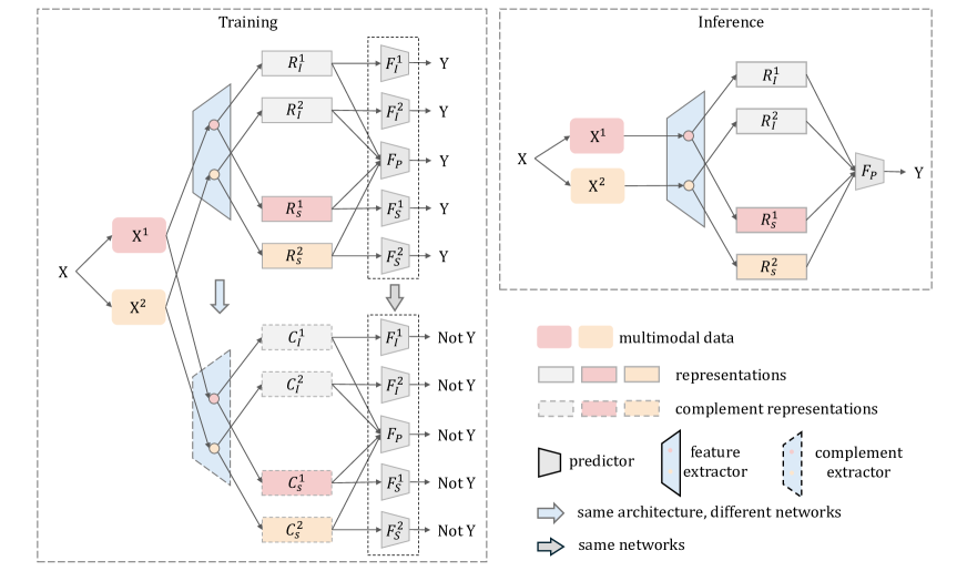
Figure 2: The architecture of a disentangle approch adapted to implement our method

Multimodal Representation Learning via PNS

Building upon our theoretical findings, we aims to obtain modality-invariant representation $R_{I}^{m}$ and modality-specific representation $R_{S}^{m}$ with high PNS values. Our approach begins by utilizing an existing disentanglement technique to extract both representations. Following this, we design objective functions that encourage learning each representation with a high PNS value while implementing constraints to ensure non-trivial PNS estimation.

Complement Representation

To evaluate PNS for multimodal representations as outlined in eq. 2 and eq. 4, we need to obtain the complement $\bar{z}$ for feature value $z$ of $Z$. This means finding complement modality-invariant representation $\mathcal{C}_{I}^{m}\subset\mathbb{R}^{d_{Z_{I}}}$ for $R_{I}^{m}$ and complement modality-specific representation $\mathcal{C}_{S}^{m}\subset\mathbb{R}^{d_{Z_{S}}}$ for $R_{S}^{m}$. Both $\mathcal{C}_{I}^{m}$ and $\mathcal{C}_{S}^{m}$ should maintain similar properties to $\mathcal{R}_{I}^{m}$ and $\mathcal{R}_{S}^{m}$, respectively, while leading to different outcome predictions. For instance, if $F_{I}^{m}(\mathcal{R}_{I}^{m})$ predicts $Y$, then $F_{I}^{m}(\mathcal{C}_{I}^{m})$ should predict a label different from $Y$.

However, it is difficult to directly obtain $\mathcal{C}_{I}^{m}$ and $\mathcal{C}_{S}^{m}$ in real-world scenario. To solve this problem, we propose using an complement extractor $\phi$ (bottom-left of fig. 2), which shares the same structure as $\Phi$ but is a separate network. $\phi$ can learn the complement representations for $X^{m}$ as:

$$[\mathcal{C}_{I}^{m},\mathcal{C}_{S}^{m}]:=\phi(X^{m})$$

In the training process, $\phi$ extracts $\mathcal{C}_{I}^{m}$ and $\mathcal{C}_{S}^{m}$ from $X^{m}$, and the auxiliary predictors are then trained to predict outcomes that differ from $Y$ based on these complement representations. The rationale is to encourage the generation of complement representations through a process analogous to the original feature extraction, preserving the underlying data structure while introducing meaningful variations.

PNS for Modality-Invariant Representation

We design the following objective to encourage $\mathcal{R}_{I}^{m}$ having a high PNS value:

$$\mathcal{L}_{m,I}^{pns}:=\mathcal{L}_{m,I}^{pred}+\mathcal{L}_{m,I}^{cf}+\mathcal{L}_{m,I}^{constr}$$ (8)

$\mathcal{L}_{m,I}^{pred}$ is defined as $\mathcal{L}_{pred}(Y,F_{I}^{m}(\mathcal{R}_{I}^{m}))$, where $\mathcal{L}_{pred}$ is a loss function that increases as $F_{I}^{m}(\mathcal{R}_{I}^{m})$ deviates from $Y$. Optimizing $\mathcal{L}_{m,I}^{pred}$ increases the probability of the prediction being close to $Y$ when the modality-invariant representation is set to $\mathcal{R}_{I}^{m}$. This aims to encourage representation to capture a high $P(Y=y\mid\text{do}(Z_{I}=z))$ in eq. 2.

$\mathcal{L}_{m,I}^{cf}$ is defined as $\mathcal{L}_{cf}(Y,F_{I}^{m}(\mathcal{C}_{I}^{m}))$, where $\mathcal{L}_{cf}$ is a loss function that increases when $F_{I}^{m}(\mathcal{C}_{I}^{m})$ is close to $Y$. Optimizing $\mathcal{L}_{m,I}^{cf}$ decreases the probability of the prediction being close to $Y$ when the modality-invariant representation is set to $\mathcal{C}_{I}^{m}$. This helps learn representations that capture a low value for $P(Y=y\mid\text{do}(Z_{I}=\bar{z}))$ in eq. 2.

The specific implementations of $\mathcal{L}_{pred}$ and $\mathcal{L}_{cf}$ may vary depending on different scenarios. We will detail our implementation in the experiment section. Together, optimizing $\mathcal{L}_{m,I}^{pred}+\mathcal{L}_{m,I}^{cf}$ represents the process of improving the PNS in eq. 2.

$\mathcal{L}_{m,I}^{constr}$ serves as a Monotonicity constraint, defined as $\mathcal{L}_{m,I}^{constr}=\mathcal{L}_{pred}(Y,F_{I}^{m}(\mathcal{R}_{I}^{m}))*\mathcal{L}_{cf}(Y,F_{I}^{m}(\mathcal{C}_{I}^{m}))$. Optimizing this term encourages representations to satisfy $P(Y_{do(Z=z)}\neq y)P(Y_{do(Z=\bar{z})}=y)=0$ in definition 3, as the multiplication of probabilities decreases when $\mathcal{L}_{m,I}^{constr}$ decreases. This aims to foster an environment where the Monotonicity is more likely to be met.

PNS for Modality-Specific Representation

Similar to eq. 8, to encourage $\mathcal{R}_{S}^{m}$ to have a high PNS value, we formulate the objective:

$$\mathcal{L}_{m,S}^{pns}:=\mathcal{L}_{m,S}^{pred}+\mathcal{L}_{m,S}^{cf}+\mathcal{L}_{m,S}^{constr}$$ (9)

$\mathcal{L}_{m,S}^{pred}$ and $\mathcal{L}_{m,S}^{cf}$ are similar to $\mathcal{L}_{m,I}^{pred}$ and $\mathcal{L}_{m,I}^{cf}$ in eq. 8. They are set as $\mathcal{L}_{pred}(Y,F_{S}^{m}(\mathcal{R}_{S}^{m}))$ and $\mathcal{L}_{cf}(Y,F_{S}^{m}(\mathcal{C}_{S}^{m}))$, respectively.

To obtain non-trival PNS, we design the constraint term $\mathcal{L}_{m,S}^{constr}=\mathcal{L}_{cf}(F_{S}^{m}(\mathcal{R}_{S}^{m}),F_{S}^{m}(\mathcal{C}_{S}^{\bar{m}}))$, where $m\neq\bar{m}$. Optimizing this term aims to increase $P(\mathcal{F}(z|m)\neq\mathcal{F}(\bar{z}|\bar{m}))$ in eq. 7 as this probability increase as $F_{S}^{m}(\mathcal{R}_{S}^{m}$) deviates from $F_{S}^{m}(\mathcal{C}_{S}^{\bar{m}})$. This aims to encourage the non-trival PNS estimation. $\mathcal{C}_{S}^{\bar{m}}$ is generated by $\phi(X^{\bar{m}})$, where $X^{m}$ and $X^{\bar{m}}$ are different modalities of the same multimodal data $X$.

Multimodal Representation Learning via Necessary and Sufficient Causes

We want the disentangling approach to learn representations with high PNS values, by optimizing the overall loss:

$$\mathcal{L}^{total}:= \mathcal{L}^{task}+\sum_{m=1}^{N}(\mathcal{L}_{m,I}^{pns}+\mathcal{L}_{m,S}^{pns})$$ (10)

$$= \mathcal{L}^{task}+\mathcal{L}^{pns}+\mathcal{L}^{constr}$$

We define $\mathcal{L}^{pns}=\sum_{m=1}^{N}(\mathcal{L}_{m,I}^{pred}+\mathcal{L}_{m,I}^{cf}+\mathcal{L}_{m,S}^{pred}+\mathcal{L}_{m,S}^{cf})$ as PNS loss term, and $\mathcal{L}^{constr}=\sum_{m=1}^{N}(\mathcal{L}_{m,I}^{constr}+\mathcal{L}_{m,S}^{constr})$ as constraint loss term. $\mathcal{L}^{task}$ is the loss for the original task of the disentangling approach. For example, it could include $\mathcal{L}_{pred}(Y,F_{P}(\mathcal{P}))$ in the multimodal prediction task.

We name our algorithm for optimizing $\mathcal{L}^{total}$ as MRLNS (Multimodal Representation Learning via Necessity and Sufficiency Causes). It builds upon an existing disentangling approach, adapting this approach to optimize $\mathcal{L}^{total}$ instead of the original $\mathcal{L}^{task}$. This adaptation involves using an complement extractor, which could be the network that mirrors the structure of the disentangling approach’s feature extractor, to generate complement representations. Then, these representations, along with the original ones, are fed into auxiliary predictors (created if not present in the chosen disentangling approach) to optimize $\mathcal{L}^{pns}+\mathcal{L}^{constr}$. During training, all components - including the feature extractor, complement extractor, predictors, and other parts of the chosen disentangling approach - are optimized. Once training is complete, the complement extractor and auxiliary predictors are discarded, leaving the trained disentangling approach ready for use, as illustrated in the top-right of fig. 2.

Experiment

We evaluate MRLNS using both synthetic and real-world datasets. First, we employ synthetic datasets to show that MRLNS can obtain representations with high PNS values. Then, we utilize real-world datasets to demonstrate MRLNS’s ability to enhance the performance of its adapted disentangling approach. All experiments are conducted on a Linux system with an NVIDIA Tesla V100 PCIe GPU.

Synthetic Dataset Experiments

Our synthetic dataset experiment aims to demonstrate MRLNS’s effectiveness in learning essential information (sufficient and necessary causes) from multimodal data. We adapt the data generation and evaluation process from (Yang et al. 2024). This process involves generating deterministic variables that directly determine the outcome, along with other variables, which are then mixed. Subsequently, representations are extracted from these mixed variables by a neural network to predict outcomes. For evaluation, we use Distance Correlation (Jones, Forrest et al. 1995) to measure how well each type of variable is captured in the learned representations. Higher correlation values indicate more relevant information captured. As deterministic variables directly influence the outcome, they possess high PNS. Consequently, a method achieving high distance correlation between deterministic variables and representations can effectively captures essential, high-PNS information.

Generating the Synthetic Dataset.

We generate a synthetic dataset based on four types of variables. These variables are used to construct a two-modality sample and its corresponding label. The variables are generated as follows:

Sufficient and Necessary (SN) cause variable $sn$ is the deterministic variable and generated from a Bernoulli distribution $B(0.5)$, with probability of 0.5 to be 1. It directly determines the label $Y$ through the relationship $Y=sn\oplus B(0.15)$, where $\oplus$ is the XOR operation.

Sufficient and Unnecessary (SF) cause variable $sf$ is generated by transforming $sn$. When $sn=0$, $sf=B(0.1)$, and when $sn=1$, $sf=sn$.

Insufficient and Necessary (NC) cause variable $nc$ is generated as $I(sn=1)\cdot B(0.9)$, where $I(\cdot)$ is indicator function.

Spurious correlation (SC) variable $sc$ is generated to have a spurious correlation with the SN cause, defined as $s\cdot sn+(1-s)\mathcal{N}(0,1)$, where $s\in[0,1)$ is the degree of spurious correlation and $\mathcal{N}(0,1)$ denotes the standard Gaussian distribution.

Based on these variables, we construct a feature vector $h=[sn\cdot\mathbf{1}_{d},sf\cdot\mathbf{1}_{d},nc\cdot\mathbf{1}_{d},sp\cdot\mathbf{1}_{d}]+\mathcal{N}(0,0.3)$, where $\mathbf{1}_{d}$ is a $d$-dimensional vector of ones and $d$ is set to 7. Following fig. 1, we create synthetic multimodal data with modality-invariant and modality-specific components. The first 3 elements of each variable serve as the modality-invariant component. For modality-specific features, we allocate the next 2 elements to modality 1 and the last 2 to modality 2. We then form temporary feature vectors $h^{1}$ and $h^{2}$ for each modality by combining the invariant component with their respective specific elements. To introduce varying complexities between two modalities, we apply a non-linear function $\kappa(t,\alpha,\beta)=\beta\cdot\max(t-\alpha,0)\cdot\min(t+\alpha,0)$. The final multimodal sample $[X^{1},X^{2},Y]$ is generated as $X^{1}=\kappa(h^{1},0.8,2.2)$ and $X^{2}=\kappa(h^{2},1,2)$.

To analyze the impact of different levels of spurious correlation on the learned representations, we vary the $s$ as 0.0, 0.1, 0.3, 0.5, and 0.7. For each value of s, we generate 15,000 samples for training and 5,000 for evaluation.

Disentangling Approach.

We refer to (Li, Wang, and Cui 2023) to design a simple disentangling network. Specifically, we construct feature extractor by exploiting a shared multimodal encoder $\mathcal{E}_{I}(\cdot)$ and two private encoders $\mathcal{E}_{S}^{1}(\cdot)$ and $\mathcal{E}_{S}^{2}(\cdot)$ to extract the disentangled representation. Formally, $\mathcal{R}_{I}^{1}=\mathcal{E}_{I}(X^{1})$, $\mathcal{R}_{I}^{2}=\mathcal{E}_{I}(X^{2})$, $\mathcal{R}_{S}^{1}=\mathcal{E}_{S}^{1}(X^{1})$, and $\mathcal{R}_{S}^{2}=\mathcal{E}_{S}^{2}(X^{2})$. The complement extractor is a separate set of encoders with the same structure as the feature extractor. All encoders, the main predictor $F_{P}$, and auxiliary predictors ($F_{I}^{1}$, $F_{I}^{2}$, $F_{S}^{1}$, and $F_{S}^{2}$) are implemented as MLP networks with hidden layers of sizes [64, 32]. We empirically use binary cross entropy for $\mathcal{L}_{pred}$ and define $\mathcal{L}_{cf}(Y,\hat{Y})=1/(\theta+|Y-\hat{Y}|)$, where $\theta=0.01$ prevents division by zero. This $\mathcal{L}_{cf}$ increases as the predicted label $\hat{Y}$ approaches the true label $Y$. Here, $\mathcal{L}_{task}$ in eq. 10 is $\mathcal{L}_{pred}(Y,F_{P}([\mathcal{R}_{I}^{1},\mathcal{R}_{I}^{2},\mathcal{R}_{S}^{1},\mathcal{R}_{S}^{2}]))$.

Table 1: Distance Correlation based on $s$ for modality 1

	Mode	SN	SF	NC	SC
s = 0.0	Net	0.600	0.647	0.635	0.269
	Net+PNS	0.608	0.652	0.545	0.261
	MRLNS	0.658	0.638	0.556	0.273
s = 0.1	Net	0.590	0.647	0.640	0.282
	Net+PNS	0.594	0.655	0.557	0.280
	MRLNS	0.675	0.613	0.565	0.285
s = 0.3	Net	0.591	0.656	0.617	0.302
	Net+PNS	0.600	0.657	0.555	0.298
	MRLNS	0.631	0.634	0.551	0.302
s = 0.5	Net	0.593	0.662	0.625	0.327
	Net+PNS	0.603	0.663	0.554	0.333
	MRLNS	0.650	0.648	0.564	0.342
s = 0.7	Net	0.594	0.653	0.640	0.326
	Net+PNS	0.610	0.653	0.562	0.327
	MRLNS	0.651	0.632	0.563	0.338

Table 2: Distance Correlation based on $s$ for modality 2

	Mode	SN	SF	NC	SC
s = 0.0	Net	0.492	0.580	0.617	0.291
	Net+PNS	0.563	0.537	0.592	0.299
	MRLNS	0.628	0.548	0.607	0.343
s = 0.1	Net	0.487	0.579	0.608	0.297
	Net+PNS	0.543	0.546	0.573	0.338
	MRLNS	0.629	0.531	0.603	0.339
s = 0.3	Net	0.492	0.591	0.591	0.325
	Net+PNS	0.564	0.546	0.584	0.359
	MRLNS	0.612	0.538	0.589	0.367
s = 0.5	Net	0.472	0.596	0.603	0.335
	Net+PNS	0.540	0.555	0.585	0.400
	MRLNS	0.601	0.545	0.602	0.388
s = 0.7	Net	0.475	0.588	0.607	0.345
	Net+PNS	0.562	0.549	0.585	0.416
	MRLNS	0.626	0.526	0.578	0.425

Results and Discussion.

The disentangling approach (denoted as Net) is trained by optimizing only $\mathcal{L}^{task}$ in eq. 10, while MRLNS is trained based on this approach by optimizing $\mathcal{L}^{total}$ in eq. 10. To evaluate their performance, for modality 1, we compute the distance correlation between the extracted representation $[\mathcal{R}_{I}^{1},\mathcal{R}_{S}^{1}]$ and each variable type (SN, SF, NC, and SC) in $X^{1}$. Similarly, for modality 2, we use $[\mathcal{R}_{I}^{2},\mathcal{R}_{S}^{2}]$ and variables in $X^{2}$. To show the effect of constraint term $\mathcal{L}^{constr}$ in eq. 10, we train a variant of MRLNS (denoted as Net+PNS) by optimizing only $\mathcal{L}^{task}+\mathcal{L}^{pns}$ in eq. 10. We run the experiment 10 times.

Table 1 and table 2 present the distance correlation values between the learned representations and the ground truth variables under varying degrees of spurious correlation ($s$).

Our analysis focuses on the results for SN, the variables that directly determines $Y$. A higher distance correlation indicates a better representation. Two tables show that MRLNS consistently outperforms both Net and Net+PNS in capturing the SN causes across various degrees of $s$ for both modalities. This demonstrates MRLNS’s effectiveness in learning representations with high PNS. While Net+PNS shows some improvement over Net, MRLNS consistently surpasses both, underscoring the importance of the full optimization objective, including the constraint term, in enforcing the learning of non-trivial PNS.

Additionally, the distance correlation with spurious information increases as $s$ increases. These results indicate that when data contains more spurious correlations, MRLNS tends to capture some of this spurious information. However, MRLNS still maintains its ability to extract SN causes effectively, which highlights the robustness of MRLNS.

Real-world Dataset Experiments

To evaluate MRLNS in real-world scenarios, we adapt an existing disentangling approach to optimize the loss of eq. 10 on multimodal datasets.

Real-world Datasets.

We utilize CMU-MOSI (Zadeh et al. 2016) and CMU-MOSEI (Zadeh et al. 2018), two widely-used datasets for multimodal emotion recognition. Both datasets provide samples labeled with sentiment scores ranging from highly negative (-3) to highly positive (3), and are available in aligned and unaligned versions. CMU-MOSI consists of 2,199 short monologue video clips, split into 1,284 training, 229 validation, and 686 testing samples. CMU-MOSEI, a larger dataset, contains 22,856 movie review video clips from YouTube, divided into 16,326 training, 1,871 validation, and 4,659 testing samples.

Disentangling Approach.

We implement MRLNS by adapting the Decoupled Multimodal Distillation (DMD) method (Li, Wang, and Cui 2023), a state-of-the-art disentangling approach. For its feature extractor, DMD uses a shared multimodal encoder to extract modality-invariant representations and private encoders for modality-specific representations from multimodal data. It then employs knowledge distillation to encourage information exchange between representations, followed by a main predictor and auxiliary predictors for outcome prediction.

Implementation of MRLNS.

To implement MRLNS, we utilize the DMD’s framework and hyper-parameters based on its publicly available code. We then add a complement extractor mirroring the architecture of DMD’s feature extractor. To optimize eq. 10, we empirically define $\mathcal{L}_{pred}$ as the mean absolute error (MAE) and $\mathcal{L}_{cf}(Y,\hat{Y})=max(0,4-||MAE(Y,\hat{Y})||)$. This $\mathcal{L}_{cf}$ increases as the predicted label $\hat{Y}$ approaches the true $Y$. $\mathcal{L}^{task}$ is the original DMD loss. By adapting DMD according to fig. 2, we create DMD+MRLNS, which optimizes the full $\mathcal{L}^{total}$ in eq. 10. To show the effect of the constraint term $\mathcal{L}^{constr}$ in eq. 10, we train DMD+PNS, a variant that optimizes only $\mathcal{L}^{task}+\mathcal{L}^{pns}$ in eq. 10.

Baselines.

We evaluate DMD, DMD+PNS, and DMD+MRLNS, and compare them with state-of-the-art methods for emotion score prediction under the same dataset settings: TFN (Zadeh et al. 2017), LMF (Liu and Shen 2018), MFM (Tsai et al. 2019), RAVEN (Wang et al. 2019), MCTN (Pham et al. 2019), and Graph-MFN (Zadeh et al. 2018). Following these works, we evaluate the performance using: (1) 7-class accuracy (Acc_7), (2) binary accuracy (Acc_2), and (3) F1 score (F1).

Results and Discussion.

The experimental results on the CMU-MOSI and CMU-MOSEI datasets are presented in table 3 and table 4, respectively. We observe that applying MRLNS to the DMD improves performance across all evaluation metrics on both datasets, regardless of whether the data is aligned or unaligned. This improvement demonstrates the effectiveness of encouraging the disentangling approach to learn high-PNS representations based on MRLNS. By focusing on features that are both necessary and sufficient for accurate predictions, the model learns more informative and discriminative representations, which in turn leads to better performance.

Furthermore, results on DMD+PNS show that removing the constraint term results in a performance drop compared to the full DMD+MRLNS model. This highlights the importance of using constraint to ensure that the multimodal representations capture the desired high-PNS properties.

Table 3: Comparison on CMU-MOSI dataset.

Aligned
Methods	Acc_7(%)	Acc_2(%)	F1(%)
TFN	32.1	73.9	73.4
LMF	32.8	76.4	75.7
MFM	36.2	78.1	78.1
RAVEN	33.2	78.0	76.6
MCTN	35.6	79.3	79.1
DMD	35.9	79.0	79.0
DMD+PNS	35.1	79.6	79.3
DMD+MRLNS	36.4	79.8	79.8
Unaligned
Methods	Acc_7(%)	Acc_2(%)	F1(%)
RAVEN	31.7	72.7	73.1
MCTN	32.7	75.9	76.4
DMD	35.9	78.8	78.9
DMD+PNS	35.4	79.3	79.4
DMD+MRLNS	36.3	79.7	79.7

Table 4: Comparison on CMU-MOSEI dataset.

Aligned
Methods	Acc_7(%)	Acc_2(%)	F1(%)
Graph-MFN	45.0	76.9	77.0
RAVEN	50.0	79.1	79.5
MCTN	49.6	79.8	80.6
DMD	51.8	83.8	83.3
DMD+PNS	52.0	83.3	83.4
DMD+MRLNS	52.2	84.4	84.2
Unaligned
Methods	Acc_7(%)	Acc_2(%)	F1(%)
RAVEN	45.5	75.4	75.7
MCTN	48.2	79.3	79.7
DMD	52.0	83.2	83.1
DMD+PNS	52.3	84.1	84.0
DMD+MRLNS	53.2	84.4	84.2

Limitation

MRLNS builds upon existing disentangling approaches to learn effective representations by incorporating PNS. However, MRLNS relies on the assumption that the representations learned by the models exhibit $\delta$-Semantic Separability. Determining the appropriate value for $\delta$ remains a challenge, as it may vary depending on the specific task and dataset. Moreover, completely and successfully disentangling the representation into modality-invariant and modality-specific components is an open problem in the field (Zhang et al. 2019; Ramachandram and Taylor 2017; Guo, Wang, and Wang 2019; Gao et al. 2020). The disentanglement process itself may introduce noise, which could affect the performance of MRLNS. Despite these limitations, we believe that MRLNS represents a novel insight in multimodal representation learning.

Conclusion

Our study identifies the key challenges in applying PNS estimation to multimodal data and propose viewing multimodal representations as comprising modality-invariant and modality-specific components to address these challenges. Building upon the theoretical derivations of PNS for these components, we develop a method that enhances multimodal models by encouraging them to learn representations with high PNS. Experiments on both synthetic and real-world datasets demonstrate the effectiveness of our method.

References

- Ahuja et al. (2020) Ahuja, K.; Shanmugam, K.; Varshney, K.; and Dhurandhar, A. 2020. Invariant risk minimization games. In International Conference on Machine Learning, 145–155. PMLR.
- Arjovsky et al. (2019) Arjovsky, M.; Bottou, L.; Gulrajani, I.; and Lopez-Paz, D. 2019. Invariant risk minimization. arXiv preprint arXiv:1907.02893.
- Cai et al. (2024) Cai, H.; Wang, Y.; Jordan, M.; and Song, R. 2024. On learning necessary and sufficient causal graphs. Advances in Neural Information Processing Systems, 36.
- Chen et al. (2024) Chen, X.; Cai, R.; Zheng, K.; Jiang, Z.; Huang, Z.; Hao, Z.; and Li, Z. 2024. Unifying Invariance and Spuriousity for Graph Out-of-Distribution via Probability of Necessity and Sufficiency. arXiv preprint arXiv:2402.09165.
- Chen et al. (2022) Chen, Y.; Zhang, Y.; Bian, Y.; Yang, H.; Kaili, M.; Xie, B.; Liu, T.; Han, B.; and Cheng, J. 2022. Learning causally invariant representations for out-of-distribution generalization on graphs. Advances in Neural Information Processing Systems, 35: 22131–22148.
- Dong et al. (2023) Dong, R.; Han, C.; Peng, Y.; Qi, Z.; Ge, Z.; Yang, J.; Zhao, L.; Sun, J.; Zhou, H.; Wei, H.; et al. 2023. DreamLLM: Synergistic Multimodal Comprehension and Creation. In The Twelfth International Conference on Learning Representations.
- Gamella and Heinze-Deml (2020) Gamella, J. L.; and Heinze-Deml, C. 2020. Active invariant causal prediction: Experiment selection through stability. Advances in Neural Information Processing Systems, 33: 15464–15475.
- Gao et al. (2020) Gao, J.; Li, P.; Chen, Z.; and Zhang, J. 2020. A survey on deep learning for multimodal data fusion. Neural Computation, 32(5): 829–864.
- Guo, Wang, and Wang (2019) Guo, W.; Wang, J.; and Wang, S. 2019. Deep multimodal representation learning: A survey. Ieee Access, 7: 63373–63394.
- Hu et al. (2018) Hu, S.; Chen, Z.; Partovi Nia, V.; Chan, L.; and Geng, Y. 2018. Causal inference and mechanism clustering of a mixture of additive noise models. Advances in neural information processing systems, 31.
- Huang et al. (2020) Huang, B.; Zhang, K.; Zhang, J.; Ramsey, J.; Sanchez-Romero, R.; Glymour, C.; and Schölkopf, B. 2020. Causal discovery from heterogeneous/nonstationary data. Journal of Machine Learning Research, 21(89): 1–53.
- Islam et al. (2023) Islam, M. M.; Gladstone, A.; Islam, R.; and Iqbal, T. 2023. EQA-MX: Embodied Question Answering using Multimodal Expression. In The Twelfth International Conference on Learning Representations.
- Jones, Forrest et al. (1995) Jones, T.; Forrest, S.; et al. 1995. Fitness distance correlation as a measure of problem difficulty for genetic algorithms. In ICGA, volume 95, 184–192.
- Li, Wang, and Cui (2023) Li, Y.; Wang, Y.; and Cui, Z. 2023. Decoupled multimodal distilling for emotion recognition. In Proceedings of the IEEE/CVF Conference on Computer Vision and Pattern Recognition, 6631–6640.
- Liang et al. (2024a) Liang, C.; Yu, J.; Yang, M.-H.; Brown, M.; Cui, Y.; Zhao, T.; Gong, B.; and Zhou, T. 2024a. Module-wise Adaptive Distillation for Multimodality Foundation Models. Advances in Neural Information Processing Systems, 36.
- Liang et al. (2024b) Liang, P. P.; Cheng, Y.; Fan, X.; Ling, C. K.; Nie, S.; Chen, R.; Deng, Z.; Allen, N.; Auerbach, R.; Mahmood, F.; et al. 2024b. Quantifying & Modeling Multimodal Interactions: An Information Decomposition Framework. Advances in Neural Information Processing Systems, 36.
- Liu et al. (2021) Liu, C.; Sun, X.; Wang, J.; Tang, H.; Li, T.; Qin, T.; Chen, W.; and Liu, T.-Y. 2021. Learning causal semantic representation for out-of-distribution prediction. Advances in Neural Information Processing Systems, 34: 6155–6170.
- Liu et al. (2024a) Liu, S.; Kimura, T.; Liu, D.; Wang, R.; Li, J.; Diggavi, S.; Srivastava, M.; and Abdelzaher, T. 2024a. FOCAL: Contrastive learning for multimodal time-series sensing signals in factorized orthogonal latent space. Advances in Neural Information Processing Systems, 36.
- Liu et al. (2024b) Liu, T.; Wang, Y.; Ying, R.; and Zhao, H. 2024b. MuSe-GNN: Learning Unified Gene Representation From Multimodal Biological Graph Data. Advances in Neural Information Processing Systems, 36.
- Liu and Shen (2018) Liu, Z.; and Shen, Y. 2018. Efficient Low-rank Multimodal Fusion with Modality-Specific Factors. In Proceedings of the 56th Annual Meeting of the Association for Computational Linguistics (Long Papers).
- Locatello et al. (2019) Locatello, F.; Bauer, S.; Lucic, M.; Raetsch, G.; Gelly, S.; Schölkopf, B.; and Bachem, O. 2019. Challenging common assumptions in the unsupervised learning of disentangled representations. In international conference on machine learning, 4114–4124. PMLR.
- Louizos et al. (2017) Louizos, C.; Shalit, U.; Mooij, J. M.; Sontag, D.; Zemel, R.; and Welling, M. 2017. Causal effect inference with deep latent-variable models. Advances in neural information processing systems, 30.
- Lu et al. (2021) Lu, C.; Wu, Y.; Hernández-Lobato, J. M.; and Schölkopf, B. 2021. Invariant causal representation learning for out-of-distribution generalization. In International Conference on Learning Representations.
- Mai, Hu, and Xing (2020) Mai, S.; Hu, H.; and Xing, S. 2020. Modality to modality translation: An adversarial representation learning and graph fusion network for multimodal fusion. In Proceedings of the AAAI Conference on Artificial Intelligence, volume 34, 164–172.
- Pearl (2009) Pearl, J. 2009. Causality. Cambridge university press.
- Peters et al. (2014) Peters, J.; Mooij, J. M.; Janzing, D.; and Schölkopf, B. 2014. Causal Discovery with Continuous Additive Noise Models. Journal of Machine Learning Research, 15(58): 2009–2053.
- Pham et al. (2019) Pham, H.; Liang, P. P.; Manzini, T.; Morency, L.-P.; and Póczos, B. 2019. Found in translation: Learning robust joint representations by cyclic translations between modalities. In Proceedings of the AAAI conference on artificial intelligence, volume 33, 6892–6899.
- Ramachandram and Taylor (2017) Ramachandram, D.; and Taylor, G. W. 2017. Deep multimodal learning: A survey on recent advances and trends. IEEE signal processing magazine, 34(6): 96–108.
- Schölkopf et al. (2021) Schölkopf, B.; Locatello, F.; Bauer, S.; Ke, N. R.; Kalchbrenner, N.; Goyal, A.; and Bengio, Y. 2021. Toward causal representation learning. Proceedings of the IEEE, 109(5): 612–634.
- Shi et al. (2019) Shi, Y.; Paige, B.; Torr, P.; et al. 2019. Variational mixture-of-experts autoencoders for multi-modal deep generative models. Advances in neural information processing systems, 32.
- Swamy et al. (2024) Swamy, V.; Satayeva, M.; Frej, J.; Bossy, T.; Vogels, T.; Jaggi, M.; Käser, T.; and Hartley, M.-A. 2024. MultiModN—Multimodal, Multi-Task, Interpretable Modular Networks. Advances in Neural Information Processing Systems, 36.
- Tang et al. (2024) Tang, J.; Du, M.; Vo, V.; Lal, V.; and Huth, A. 2024. Brain encoding models based on multimodal transformers can transfer across language and vision. Advances in Neural Information Processing Systems, 36.
- Tran et al. (2024) Tran, M.; Dicente Cid, Y.; Lahiani, A.; Theis, F.; Peng, T.; and Klaiman, E. 2024. Training Transitive and Commutative Multimodal Transformers with LoReTTa. Advances in Neural Information Processing Systems, 36.
- Tsai et al. (2018) Tsai, Y.-H. H.; Liang, P. P.; Zadeh, A.; Morency, L.-P.; and Salakhutdinov, R. 2018. Learning Factorized Multimodal Representations. In International Conference on Learning Representations.
- Tsai et al. (2019) Tsai, Y.-H. H.; Liang, P. P.; Zadeh, A.; Morency, L.-P.; and Salakhutdinov, R. 2019. Learning Factorized Multimodal Representations. In International Conference on Representation Learning.
- Wang et al. (2017) Wang, B.; Yang, Y.; Xu, X.; Hanjalic, A.; and Shen, H. T. 2017. Adversarial cross-modal retrieval. In Proceedings of the 25th ACM international conference on Multimedia, 154–162.
- Wang and Jordan (2021) Wang, Y.; and Jordan, M. I. 2021. Desiderata for representation learning: A causal perspective. arXiv preprint arXiv:2109.03795.
- Wang et al. (2019) Wang, Y.; Shen, Y.; Liu, Z.; Liang, P. P.; Zadeh, A.; and Morency, L.-P. 2019. Words can shift: Dynamically adjusting word representations using nonverbal behaviors. In Proceedings of the AAAI Conference on Artificial Intelligence, volume 33, 7216–7223.
- Xu et al. (2024) Xu, A.; Hou, Y.; Niell, C.; and Beyeler, M. 2024. Multimodal Deep Learning Model Unveils Behavioral Dynamics of V1 Activity in Freely Moving Mice. Advances in Neural Information Processing Systems, 36.
- Yang et al. (2024) Yang, M.; Zhang, Y.; Fang, Z.; Du, Y.; Liu, F.; Ton, J.-F.; Wang, J.; and Wang, J. 2024. Invariant learning via probability of sufficient and necessary causes. Advances in Neural Information Processing Systems, 36.
- Yang et al. (2021) Yang, S.; Yu, K.; Cao, F.; Liu, L.; Wang, H.; and Li, J. 2021. Learning causal representations for robust domain adaptation. IEEE Transactions on Knowledge and Data Engineering, 35(3): 2750–2764.
- Zadeh et al. (2017) Zadeh, A.; Chen, M.; Poria, S.; Cambria, E.; and Morency, L.-P. 2017. Tensor Fusion Network for Multimodal Sentiment Analysis. In Proceedings of the 2017 Conference on Empirical Methods in Natural Language Processing. Association for Computational Linguistics.
- Zadeh et al. (2016) Zadeh, A.; Zellers, R.; Pincus, E.; and Morency, L.-P. 2016. Multimodal sentiment intensity analysis in videos: Facial gestures and verbal messages. IEEE Intelligent Systems, 31(6): 82–88.
- Zadeh et al. (2018) Zadeh, A. B.; Liang, P. P.; Poria, S.; Cambria, E.; and Morency, L.-P. 2018. Multimodal language analysis in the wild: Cmu-mosei dataset and interpretable dynamic fusion graph. In Proceedings of the 56th Annual Meeting of the Association for Computational Linguistics (Volume 1: Long Papers), 2236–2246.
- Zhang et al. (2020) Zhang, A.; Lyle, C.; Sodhani, S.; Filos, A.; Kwiatkowska, M.; Pineau, J.; Gal, Y.; and Precup, D. 2020. Invariant causal prediction for block mdps. In International Conference on Machine Learning, 11214–11224. PMLR.
- Zhang et al. (2019) Zhang, S.-F.; Zhai, J.-H.; Xie, B.-J.; Zhan, Y.; and Wang, X. 2019. Multimodal representation learning: Advances, trends and challenges. In 2019 International Conference on Machine Learning and Cybernetics (ICMLC), 1–6. IEEE.
- Zhang, Kong, and Zhou (2023) Zhang, Y.; Kong, Q.; and Zhou, F. 2023. Integration-free Training for Spatio-temporal Multimodal Covariate Deep Kernel Point Processes. Advances in Neural Information Processing Systems, 36: 25031–25049.
- Zheng et al. (2018) Zheng, X.; Aragam, B.; Ravikumar, P. K.; and Xing, E. P. 2018. Dags with no tears: Continuous optimization for structure learning. Advances in neural information processing systems, 31.
- Zhu, Ng, and Chen (2019) Zhu, S.; Ng, I.; and Chen, Z. 2019. Causal discovery with reinforcement learning. arXiv preprint arXiv:1906.04477.