An Adaptive Latent Factorization of Tensors Model for Embedding Dynamic Communication Network

Abstract

The Dynamic Communication Network (DCN) describes the interactions over time among various communication nodes, and it is widely used in Big-data applications as a data source. As the number of communication nodes increases and temporal slots accumulate, each node interacts in with only a few nodes in a given temporal slot, the DCN can be represented by an High-Dimensional Sparse (HDS) tensor. In order to extract rich behavioral patterns from an HDS tensor in DCN, this paper proposes an Adaptive Temporal-dependent Tensor low-rank representation (ATT) model. It adopts a three-fold approach: a) designing a temporal-dependent method to reconstruct temporal feature matrix, thereby precisely represent the data by capturing the temporal patterns; b) achieving hyper-parameters adaptation of the model via the Differential Evolutionary Algorithms (DEA) to avoid tedious hyper-parameters tuning; c) employing nonnegative learning schemes for the model parameters to effectively handle an the nonnegativity inherent in HDS data. The experimental results on four real-world DCNs demonstrate that the proposed ATT model significantly outperforms several state-of-the-art models in both prediction errors and convergence rounds.

I Introduction

With the rapid advancement of the internet and communication technology [1, 2, 3], the information transmission among a great number of communication devices such as computers, mobile devices, etc. generates intricate dynamic interactions, which can be effectively depicted by an Dynamic Communication Network [4] (DCN). Specifically, each node in a communication network denotes a communication device, links between nodes denote interaction behaviors, and weights on the links quantify interactions’ strength. Further, the DCN is obtained by stacking the communication networks in different temporal slots chronologically, which contains rich behavioral patterns of the involved nodes [5]. However, as the number of nodes increases dramatically and temporal slots accumulate heavily [6], it is impossible for all nodes to build interaction behaviors in all temporal slots, and only partial node interactions are observed in few temporal slots, which results in DCNs that are High-Dimensional Sparse [7, 8, 9, 10, 11, 12, 13, 14] (HDS). Therefore, how to precisely extract the required knowledge from an HDS tensor becomes a tricky task.

Researchers have proposed a variety of different analysis approaches to a DCN for exploring behavioral and temporal patterns [15, 16, 17, 18, 19, 20, 21, 22, 23, 24, 25, 26], such as Matrix Factorization models, Ma et al. [27] divide the tensor into different matrix slices and use respectively nonnegative matrix factorization to analyze the dynamic data; Graph Neural Network (GNN) models [28], Zhang et al. [29] propose a relational GNN to analyze dynamic graphs by using neighborhood information; Recurrent Neural Network (RNN) models, Jiao et al. [30] propose an RNN embedding method based on a variational auto-encoder; and Generative Adversarial Network (GAN) models, Ren et al. [31] propose a fully data-driven GAN for dynamic data imputation. Although the above models are proven to be effective for the DCN analysis, their expensive computational and storage overheads limit their generalization to large-scale real-world applications.

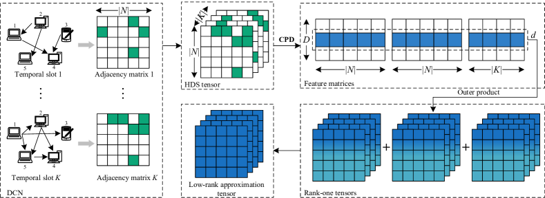
Figure 1: A low-rank representation of HDS tensor constructed by a DCN.

Previous studies [32, 33, 34, 35, 36, 37, 38, 39, 40, 41, 42] demonstrate that the Tensors Low-rank Representation (TLR) models can precisely extract pattern information from HDS data by preserving the spatio-temporal structure of a DCN, thereby effectively performing behavioral and temporal pattern analysis. Therefore, this paper proposes an Adaptive Temporal-dependent Tensor low-rank representation (ATT) model to perform DCNs analysis, which employs a Temporal-dependent Weight Matrix (TWM) and a Differential Evolutionary Algorithm [43, 44] (DEA) to provide excellent model performance. The main contributions of this paper are provided as follows:

• A TWM-based approach. It considers the correlations between temporal slots to achieve lower prediction errors.

• A DEA-based hyper-parameters adaptation scheme. It automatically adjusts the best hyper-parameters during parameter learning to achieve fast model convergence.

• Extensive experimental evaluation on four real-world DCNs datasets. It indicates that the ATT model has better model performance in terms of prediction errors and convergence rounds.

For the remained sections, Section II presents the Background and Section III introduces the proposed ATT model in detail. In addition, SectionIV shows the comparison experiments between ATT and competing models and Section V provides the conclusions and future works.

II Background

II-A Symbol Definitions

TABLE I: The description for symbol definitions

Symbol	Definition
$N,K$	The node and temporal slot sets.
$\textbf{X}\in\mathbb{R}_{+}^{N\times N\times K}$	The HDS tensor constructed via a DCN.
$\tilde{\textbf{X}}\in\mathbb{R}_{+}^{N\times N\times K}$	The low-rank approximation tensor of X.
$\textbf{R}\in\mathbb{R}_{+}^{N\times N\times K}$	The rank-one tensor for $\tilde{\textbf{X}}$.
$x_{ijk},\tilde{x}_{ijk},r_{ijk}$	The single element of $\textbf{X},\tilde{\textbf{X}}$, and R.
$D$	The number of rank-one tensors.
$\{\mathrm{S},\mathrm{U}\}\in\mathbb{R}_{+}^{N\times D}$	The node feature matrices
$\mathrm{Z}\in\mathbb{R}_{+}^{K\times D}$	The temporal feature matrix
$\textbf{{s}}_{d},\textbf{{u}}_{d},\textbf{{z}}_{d}$	The $d$-th column vectors of S, U, and Z.
$s_{id},u_{jd},z_{kd}$	The single element of S, U, and Z.
$\mathrm{W}\in\mathbb{R}_{+}^{K\times K}$	The TWM.
$\{\textbf{{a}},\textbf{{c}}\}\in\mathbb{R}_{+}^{N},\textbf{{e}}\in\mathbb{R}_{+}^{K}$	The node and temporal bias vectors
$a_{i},c_{j},e_{k}$	The single element of a, c, and e.

The symbol definitions of this paper are listed in Table I.

II-B Problem Formulation

As illustrated in Fig. 1, the communication network for each temporal slot is represented by the corresponding adjacency matrix and a third-order tensor can be constructed by stacking the adjacency matrices along the temporal dimension.

Definition 1: Let $\Omega$ and $\Upsilon$ denote the observed and unobserved element sets for a tensor X, respectively. If $|\Upsilon|\gg|\Omega|$, X is an HDS tensor [45], where each element $x_{ijk}\in\textbf{X}$ denotes the interaction weight between the communication nodes $i\in N$ and $j\in N$ at the temporal slot $k\in K$.

Therefore, following the principle of Canonical Polyadic Decomposition [46] (CPD), the HDS tensor X is decomposed into three feature matrices $\mathrm{S},\mathrm{U}$, and $\mathrm{Z}$ by the low-rank representation approach. With it, the low-rank approximation $\tilde{\textbf{X}}$ of X contains the $D$ rank-one tensors as:

$$\tilde{\textbf{X}}=\sum\limits_{d=1}^{D}{{\textbf{R}_{d}}},$$ (1)

where a rank-one tensor $\textbf{R}_{d}$ is formed by the $d$-th row vector of the three feature matrices $\mathbf{R}_{d}=\textbf{{s}}_{d}\circ\textbf{{u}}_{d}\circ\textbf{{z}}_{d}$. Further, we can obtain a fine-grained single element $\tilde{x}_{ijk}$ as following:

$${\tilde{x}_{ijk}}=\sum\limits_{d=1}^{D}{r_{ijk}^{(d)}}=\sum\limits_{d=1}^{D}{{s_{id}}{u_{jd}}{z_{kd}}}.$$ (2)

By previous studies [17, 47, 48, 49, 50, 51, 52, 53, 54, 55], incorporating the corresponding bias $\textbf{{a}},\textbf{{c}}$, and e can effectively suppress the fluctuation of HDS data over time. Hence, $\tilde{x}_{ijk}$ is reformulated as below:

$${\tilde{x}_{ijk}}=\sum\limits_{d=1}^{D}{{s_{id}}{u_{jd}}{z_{kd}}}+a_{i}+c_{j}+e_{k}.$$ (3)

In order to obtain the desired feature matrices and bias vectors, it is common to employ the Euclidean distance [56, 57, 58, 12, 59, 60, 61, 62, 63, 64] to model the gap between the original tensor X and the lower-order approximation tensor $\tilde{\textbf{X}}$. Note that the original tensor is HDS, it is efficient to measure the gap on observed data $\Omega$ in X. Meanwhile, we adopt $L_{2}$ norm-based regularization [65, 66, 67, 68, 69, 70, 71, 72] to avoid model overfitting. Therefore, the objective function $\varepsilon$ is constructed as follows:

$$\begin{array}[]{l}\varepsilon=\frac{1}{2}\sum\limits_{\Omega}{{{\left({{x_{ijk}}-\sum\limits_{d=1}^{D}{{s_{id}}{u_{jd}}{z_{kd}}}-{a_{i}}-{c_{j}}-{e_{k}}}\right)}^{2}}}\\ +\frac{1}{2}\sum\limits_{\Omega}{{\left({\lambda\sum\limits_{d=1}^{D}{\left({s_{id}^{2}+u_{jd}^{2}+z_{kd}^{2}}\right)}+{\lambda_{b}}\left({a_{i}^{2}+c_{j}^{2}+e_{k}^{2}}\right)}\right)}},\end{array}$$ (4)

where $\lambda$ and $\lambda_{b}$ denote the regularization constant of controlling feature matrices and bias vectors, respectively. $\Omega$ denote the observed data on HDS tensor X. Moreover, since the HDS data in the DCN is nonnegative, it is necessary to incorporate constraints for feature matrices and bias vectors to accurately characterize the data’s nonnegativity as:

$$\begin{array}[]{l}\varepsilon=\frac{1}{2}\sum\limits_{\Omega}{{{\left({{x_{ijk}}-\sum\limits_{d=1}^{D}{{s_{id}}{u_{jd}}{z_{kd}}}-{a_{i}}-{c_{j}}-{e_{k}}}\right)}^{2}}}\\ +\frac{1}{2}\sum\limits_{\Omega}{{\left({\lambda\sum\limits_{d=1}^{D}{\left({s_{id}^{2}+u_{jd}^{2}+z_{kd}^{2}}\right)}+{\lambda_{b}}\left({a_{i}^{2}+c_{j}^{2}+e_{j}^{2}}\right)}\right)}},\\ s.t.\forall i\in N,\forall j\in N,\forall k\in K,\forall d\in\{1\sim D\}:\\ {s_{id}}\geq 0,{u_{jd}}\geq 0,{z_{kd}}\geq 0,{a_{i}}\geq 0,{c_{j}}\geq 0,{e_{k}}\geq 0.\end{array}$$ (5)

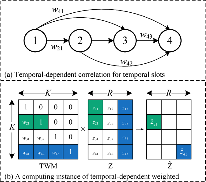
Figure 2: An illustration of the temporal-dependent.

III ATT model

III-A Objective Function

As mentioned previously, the DCN is time-varying in nature, and there is a specific influence between the temporal slots $k$ and $k+1$, i.e., subsequent communication interactions are influenced by previous interaction situations, as shown in Fig. 2(a). Therefore, we design a TWM $\mathrm{W}$ to learn the correlation between temporal slots, which reacts to the learning process of the temporal feature matrix and bias vector. Fig. 2(b) presents the computing instance between the temporal feature matrix and TWM, with the same computing for the temporal bias vector, they are given as:

$${\hat{z}_{kd}}=\sum\limits_{l=1}^{k}{{w_{kl}}{z_{ld}}},\quad{\hat{e}_{k}}=\sum\limits_{l=1}^{k}{{w_{kl}}{e_{l}}}.$$ (6)

Note that for the learnable TWM, $w_{kl}=0,l>k$ since subsequent temporal information does not influence the previous interactions. Also, the diagonal weights are set to $w_{kk}=1$ since the temporal slot $k$ has a constant correlation with itself. Therefore, the temporal-dependent objective function is reformulated as follows:

$$\begin{array}[]{*{20}{l}}{\varepsilon=\frac{1}{2}\sum\limits_{\Omega}{{{\left({{x_{ijk}}-\sum\limits_{d=1}^{D}{{s_{id}}{u_{jd}}{{\hat{z}}_{kd}}}-{a_{i}}-{c_{j}}-{{\hat{e}}_{k}}}\right)}^{2}}}}\\ {+\frac{1}{2}\sum\limits_{\Omega}{\left({\lambda\sum\limits_{d=1}^{D}{\left({s_{id}^{2}+u_{jd}^{2}+\hat{z}_{kd}^{2}}\right)}+{\lambda_{b}}\left({a_{i}^{2}+c_{j}^{2}+\hat{e}_{k}^{2}}\right)}\right)},}\\ {s.t.\forall i\in N,\forall j\in N,\forall k\in K,\forall d\in\{1\sim D\}:}\\ {{s_{id}}\geq 0,{u_{jd}}\geq 0,{z_{ld}}\geq 0,{a_{i}}\geq 0,{c_{j}}\geq 0,{e_{l}}\geq 0,{w_{kl}}\geq 0.}\end{array}$$ (7)

III-B Parameters Learning

In order to learn the desired feature matrices, bias vectors, and learnable weight matrix, we firstly adopt the Additive Gradient Descent (AGD) approach [73, 74, 75, 76] to implement their learning scheme as:

$$\begin{array}[]{l}\left({\mathrm{S},\mathrm{U},\mathrm{Z},\textbf{{a}},\textbf{{c}},\textbf{{e}},\mathrm{W}}\right)=\mathop{\arg\min}\limits_{\mathrm{S},\mathrm{U},\mathrm{Z},\textbf{{a}},\textbf{{c}},\textbf{{e}},\mathrm{W}}\varepsilon\mathop{\Rightarrow}\limits^{\mathrm{AGD}}\\ \left\{\begin{array}[]{l}{s_{id}}\leftarrow{s_{id}}-{\eta_{id}}\frac{{\partial\varepsilon}}{{\partial{s_{id}}}}={s_{id}}\\ \quad\;-{\eta_{id}}\sum\limits_{{\Omega_{\left(i\right)}}}{\left({\left({{x_{ijk}}-{{\tilde{x}}_{ijk}}}\right)\left({-{u_{jd}}{{\hat{z}}_{kd}}}\right)+\lambda{s_{id}}}\right)};\\ {z_{ld}}\leftarrow{z_{ld}}-{\eta_{ld}}\frac{{\partial\varepsilon}}{{\partial{{\hat{z}}_{kd}}}}\frac{{\partial{{\hat{z}}_{kd}}}}{{\partial{z_{ld}}}}={z_{ld}}\\ \quad\;-{\eta_{ld}}\sum\limits_{{\Omega_{\left(k\right)}}}{\left({\left({\left({{x_{ijk}}-{{\tilde{x}}_{ijk}}}\right)\left({-{s_{id}}{u_{jd}}}\right)+\lambda{{\hat{z}}_{kd}}}\right){w_{kl}}}\right)};\\ {a_{i}}\leftarrow{a_{i}}-{\eta_{i}}\sum\limits_{{\Omega_{\left(i\right)}}}{\left({-\left({{x_{ijk}}-{{\tilde{x}}_{ijk}}}\right)+{\lambda_{b}}{a_{i}}}\right)};\\ {e_{l}}\leftarrow{e_{l}}-{\eta_{l}}\sum\limits_{{\Omega_{\left(k\right)}}}{\left({\left({-\left({{x_{ijk}}-{{\tilde{x}}_{ijk}}}\right)+{\lambda_{b}}{{\hat{e}}_{k}}}\right){w_{kl}}}\right)};\\ {w_{kl}}\leftarrow{w_{kl}}-{\eta_{kl}}\left({\frac{{\partial\varepsilon}}{{\partial{{\hat{z}}_{kd}}}}\frac{{\partial{{\hat{z}}_{kd}}}}{{\partial{w_{kl}}}}+\frac{{\partial\varepsilon}}{{\partial{{\hat{e}}_{k}}}}\frac{{\partial{{\hat{e}}_{k}}}}{{\partial{w_{kl}}}}}\right)={w_{kl}}\\ \quad\;-{\eta_{kl}}\sum\limits_{{\Omega_{\left(k\right)}}}{\left({\left({\left({{x_{ijk}}-{{\tilde{x}}_{ijk}}}\right)\left({-{s_{id}}{u_{jd}}}\right)+\lambda{{\hat{z}}_{kd}}}\right){z_{ld}}}\right)}\\ \quad\;-{\eta_{kl}}\sum\limits_{{\Omega_{\left(k\right)}}}{\left({\left({-\left({{x_{ijk}}-{{\tilde{x}}_{ijk}}}\right)+{\lambda_{b}}{{\hat{e}}_{k}}}\right){e_{l}}}\right)},\end{array}\right.\end{array}$$ (8)

where $\eta_{id}$, $\eta_{ld}$, $\eta_{i}$, $\eta_{l}$, and $\eta_{kl}$ are the learning rates of $s_{id},z_{ld},a_{i},e_{l}$, and $w_{kl}$, respectively. $\Omega_{\left(i\right)}$ and $\Omega_{\left(k\right)}$ denote the subsets of $\Omega$ linked with $i\in N$ and $k\in K$, respectively. Note that applying AGD approach directly doesn’t satisfy the nonnegativity condition in the objective function. Therefore, we follow the principle of Nonnegative Multiplication Update [77, 78, 79] (NMU) to adjust the learning rate as follows:

$$\left\{\begin{array}[]{l}{\eta_{id}}={{{s_{id}}}\mathord{\left/{\vphantom{{{s_{id}}}{\sum\limits_{{\Omega_{\left(i\right)}}}{\left({{{\tilde{x}}_{ijk}}{u_{jd}}{{\hat{z}}_{kd}}+\lambda{s_{ir}}}\right)}}}}\right.\kern-1.2pt}{\sum\limits_{{\Omega_{\left(i\right)}}}{\left({{{\tilde{x}}_{ijk}}{u_{jd}}{{\hat{z}}_{kd}}+\lambda{s_{ir}}}\right)}}};\\ {\eta_{ld}}={{{z_{ld}}}\mathord{\left/{\vphantom{{{z_{ld}}}{\sum\limits_{{\Omega_{\left(k\right)}}}{\left({{{\tilde{x}}_{ijk}}{s_{id}}{u_{jd}}+\lambda{{\hat{z}}_{kd}}}\right){w_{kl}}}}}}\right.\kern-1.2pt}{\sum\limits_{{\Omega_{\left(k\right)}}}{\left({{{\tilde{x}}_{ijk}}{s_{id}}{u_{jd}}+\lambda{{\hat{z}}_{kd}}}\right){w_{kl}}}}};\\ {\eta_{i}}={{{a_{i}}}\mathord{\left/{\vphantom{{{a_{i}}}{\sum\limits_{{\Omega_{\left(i\right)}}}{\left({{{\tilde{x}}_{ijk}}+{\lambda_{b}}{a_{i}}}\right)}}}}\right.\kern-1.2pt}{\sum\limits_{{\Omega_{\left(i\right)}}}{\left({{{\tilde{x}}_{ijk}}+{\lambda_{b}}{a_{i}}}\right)}}};\\ {\eta_{l}}={{{e_{l}}}\mathord{\left/{\vphantom{{{e_{l}}}{\sum\limits_{{\Omega_{\left(k\right)}}}{\left({{{\tilde{x}}_{ijk}}+{\lambda_{b}}{{\hat{e}}_{k}}}\right){w_{kl}}}}}}\right.\kern-1.2pt}{\sum\limits_{{\Omega_{\left(k\right)}}}{\left({{{\tilde{x}}_{ijk}}+{\lambda_{b}}{{\hat{e}}_{k}}}\right){w_{kl}}}}};\\ {\eta_{kl}}={{{w_{kl}}}\mathord{\left/{\vphantom{{{w_{kl}}}{\sum\limits_{{\Omega_{\left(k\right)}}}{\left({{{\tilde{x}}_{ijk}}{s_{id}}{u_{jd}}+\lambda{{\hat{z}}_{kd}}}\right){z_{ld}}+\left({{{\tilde{y}}_{ijk}}+{\lambda_{b}}{{\hat{e}}_{k}}}\right){e_{l}}}}}}\right.\kern-1.2pt}{\sum\limits_{{\Omega_{\left(k\right)}}}{\left({{{\tilde{x}}_{ijk}}{s_{id}}{u_{jd}}+\lambda{{\hat{z}}_{kd}}}\right){z_{ld}}+\left({{{\tilde{y}}_{ijk}}+{\lambda_{b}}{{\hat{e}}_{k}}}\right){e_{l}}}}}.\end{array}\right.$$ (9)

By submitting the learning rates in (9) to the learning scheme in (8), we can obtain the following nonnegative update rules:

$$\left\{\begin{array}[]{l}{s_{id}}\leftarrow{{{s_{id}}\sum\limits_{{\Omega_{\left(i\right)}}}{{x_{ijk}}{u_{jd}}{{\hat{z}}_{kd}}}}\mathord{\left/{\vphantom{{{s_{id}}\sum\limits_{{\Omega_{\left(i\right)}}}{{x_{ijk}}{u_{jd}}{{\hat{z}}_{kd}}}}{\sum\limits_{{\Omega_{\left(i\right)}}}{{{\tilde{x}}_{ijk}}{u_{jd}}{{\hat{z}}_{kd}}+\lambda{s_{id}}}}}}\right.\kern-1.2pt}{\sum\limits_{{\Omega_{\left(i\right)}}}{{{\tilde{x}}_{ijk}}{u_{jd}}{{\hat{z}}_{kd}}+\lambda{s_{id}}}}};\\ {z_{ld}}\leftarrow{{{z_{ld}}\sum\limits_{{\Omega_{\left(k\right)}}}{\left({{x_{ijk}}{s_{id}}{u_{jd}}}\right)}}\mathord{\left/{\vphantom{{{z_{ld}}\sum\limits_{{\Omega_{\left(k\right)}}}{\left({{x_{ijk}}{s_{id}}{u_{jd}}}\right)}}{\sum\limits_{{\Omega_{\left(k\right)}}}{\left({{{\tilde{x}}_{ijk}}{s_{id}}{u_{jd}}+\lambda{{\hat{z}}_{kd}}}\right)}}}}\right.\kern-1.2pt}{\sum\limits_{{\Omega_{\left(k\right)}}}{\left({{{\tilde{x}}_{ijk}}{s_{id}}{u_{jd}}+\lambda{{\hat{z}}_{kd}}}\right)}}};\\ {a_{i}}\leftarrow{{{a_{i}}\sum\limits_{{\Omega_{\left(i\right)}}}{{x_{ijk}}}}\mathord{\left/{\vphantom{{{a_{i}}\sum\limits_{{\Omega_{\left(i\right)}}}{{x_{ijk}}}}{\sum\limits_{{\Omega_{\left(i\right)}}}{{{\tilde{x}}_{ijk}}+{\lambda_{b}}{a_{i}}}}}}\right.\kern-1.2pt}{\sum\limits_{{\Omega_{\left(i\right)}}}{{{\tilde{x}}_{ijk}}+{\lambda_{b}}{a_{i}}}}};\\ {e_{l}}\leftarrow{{{e_{l}}\sum\limits_{{\Omega_{\left(k\right)}}}{{x_{ijk}}}}\mathord{\left/{\vphantom{{{e_{l}}\sum\limits_{{\Omega_{\left(k\right)}}}{{x_{ijk}}}}{\sum\limits_{{\Omega_{\left(k\right)}}}{\left({{{\tilde{x}}_{ijk}}+{\lambda_{b}}{{\hat{e}}_{k}}}\right)}}}}\right.\kern-1.2pt}{\sum\limits_{{\Omega_{\left(k\right)}}}{\left({{{\tilde{x}}_{ijk}}+{\lambda_{b}}{{\hat{e}}_{k}}}\right)}}};\\ {w_{kl}}\leftarrow{{{w_{kl}}\sum\limits_{{\Omega_{\left(k\right)}}}{\left({{x_{ijk}}{s_{id}}{u_{jd}}}\right){z_{ld}}+{x_{ijk}}{e_{l}}}}\mathord{\left/{\vphantom{{{w_{kl}}\sum\limits_{{\Omega_{\left(k\right)}}}{\left({{x_{ijk}}{s_{id}}{u_{jd}}}\right){z_{ld}}+{x_{ijk}}{e_{l}}}}{}}}\right.\kern-1.2pt}}{}\\ \quad\quad\;\;\;\sum\limits_{{\Omega_{\left(k\right)}}}{\left({{{\tilde{x}}_{ijk}}{s_{id}}{u_{jd}}+\lambda{{\hat{z}}_{kd}}}\right){z_{ld}}+\left({{{\tilde{y}}_{ijk}}+{\lambda_{b}}{{\hat{e}}_{k}}}\right){e_{l}}}.\end{array}\right.$$ (10)

With (10), it is demonstrated that if the parameters of ATT are initialized to be nonnegative, then they remain nonnegative during the learning process, thereby satisfying the constraints in the objective function.

III-C The DEA-based Hyper-parameters Adaptation

As presented in the previous section, the learning rule for the model parameters relies on two hyper-parameters $\lambda$ and $\lambda_{b}$, which significantly affect the effectiveness of parameters learning. How to choose the appropriate hyper-parameters is a crucial step. To avoid the time and computational overhead of manually adjusting the hyperparameters, we adopt the DEA to achieve hyper-parameters adaptation due to the simple structure and excellent global convergence characteristics of DEA. Specifically, we initialize $P$ individuals as a swarm, where the $p$-th individual is defined as a vector $\textbf{{v}}_{(p)}=(\lambda_{(p)},\lambda_{b(p)})$, $p=1,...,P$, it’s given as:

$${\textbf{{v}}_{\left(p\right)}}=\left\{\begin{array}[]{l}{\lambda_{\left(p\right)}}={\lambda^{\min}}+\theta\left({{\lambda^{\max}}-{\lambda^{\min}}}\right);\\ {\lambda_{b\left(p\right)}}=\lambda_{b}^{\min}+\theta\left({\lambda_{b}^{\max}-\lambda_{b}^{\min}}\right),\end{array}\right.$$ (11)

where $(\lambda^{\min},\lambda^{\max})$ and $(\lambda_{b}^{\min},\lambda_{b}^{\max})$ are the lower and upper bounds of $\lambda$ and $\lambda_{b}$, respectively. $\theta$ is a random value in the range $[0,1]$. Following the principle of DEA, each individual is performed the mutation operation as follows:

$$\textbf{{v}}_{\left(p\right)}^{t+1}=\boldsymbol{\tau}+\mu\left({\textbf{{v}}_{\left({r1}\right)}^{t}-\textbf{{v}}_{\left({r2}\right)}^{t}}\right),$$ (12)

where $\boldsymbol{\tau}$ is the global best individual, $\mu$ is the scaling factor, $r_{1}$ and $r_{2}$ are two randomly selected individuals. Note that each individual is bounded via (13) as:

$${\textbf{{v}}^{t+1}_{\left(p\right)}}=\left\{\begin{array}[]{l}{\lambda^{\min}}\leq{\lambda^{t+1}_{\left(p\right)}}\leq{\lambda^{\max}};\\ \lambda_{b}^{\min}\leq{\lambda^{t+1}_{b\left(p\right)}}\leq\lambda_{b}^{\max}.\end{array}\right.$$ (13)

After that, each individual is performed the crossover operation as below:

$$\textbf{{v}}_{m\left(p\right)}^{t+1}=\left\{\begin{array}[]{l}\textbf{{v}}_{m\left(p\right)}^{t+1};\quad{\rm{if}}\;\theta\leq{C_{p}}\;{\rm{or}}\;m={m^{*}}\\ \textbf{{v}}_{m\left(p\right)}^{t},\quad{\rm{else}}\end{array}\right.$$ (14)

where $m\in\mathbb{N}$ denotes one of the dimensions in vector $\textbf{{v}}_{(p)}$, $C_{p}\in[0,1]$ denotes the crossover probability, and $m^{*}$ denotes a randomly selected dimension. Next, each individual is evaluated for fitness by the learning process of the model parameters, and the fitness function $F$ for the $t$-th iteration is defined as:

$$F_{(p)}^{t+1}=\frac{{H\left({\textbf{{v}}_{(p)}^{t+1}}\right)-H\left({\textbf{{v}}_{(p-1)}^{t+1}}\right)}}{{H\left({\textbf{{v}}_{(P)}^{t+1}}\right)-H\left({\textbf{{v}}_{(P)}^{t}}\right)}},$$ (15)

where $H(\textbf{{v}}^{t+1}_{(0)})=H(\textbf{{v}}^{(t)}_{P})$ and $H$ is calculated by the current performance of the model parameters, it’s given as:

$$H\left({{\textbf{{v}}_{(p)}}}\right)=\sqrt{\frac{{\sum\limits_{\Lambda}{{{\left({{x_{ijk}}-{{\tilde{x}}_{ijk\left(p\right)}}}\right)}^{2}}}}}{{4\left|\Lambda\right|}}}+\;\frac{{\sum\limits_{\Lambda}{{{\left|{{x_{ijk}}-{{\tilde{x}}_{ijk\left(p\right)}}}\right|}_{a}}}}}{{2\left|\Lambda\right|}},$$ (16)

where $\Lambda$ denotes the validation set form $\Omega$ and $|\cdot|_{a}$ denotes the absolute value. Note that the approximation $\tilde{x}_{ijk}$ in (16) is calculated via the current model parameters. takes $(s_{id},a_{i})$ and as an example, their learning rules are as follows:

$$\left\{\begin{array}[]{l}{s_{id\left(p\right)}}\leftarrow\frac{{{s_{id\left(p\right)}}\sum\limits_{{\Omega_{\left(i\right)}}}{{x_{ijk}}{u_{jd}}{{\hat{z}}_{kd}}}}}{{\sum\limits_{{\Omega_{\left(i\right)}}}{{{\tilde{x}}_{ijk\left(p\right)}}{u_{jd\left(p\right)}}{{\hat{z}}_{kd\left(p\right)}}+{\lambda_{\left(p\right)}}{s_{id\left(p\right)}}}}};\\ {a_{i\left(p\right)}}\leftarrow\frac{{{a_{i\left(p\right)}}\sum\limits_{{\Omega_{\left(i\right)}}}{{x_{ijk}}}}}{{\sum\limits_{{\Omega_{\left(i\right)}}}{{{\tilde{x}}_{ijk\left(p\right)}}+{\lambda_{b\left(p\right)}}{a_{i\left(p\right)}}}}}.\end{array}\right.$$ (17)

By the evaluation of fitness functions, the global best individual is updated as below:

$${\boldsymbol{\tau}^{t+1}}=\left\{{\begin{array}[]{*{20}{c}}{{\boldsymbol{\tau}^{t}},F_{(p)}^{t+1}\leq F_{(p-1)}^{t+1},}\\ {\textbf{{v}}_{(p)}^{t+1},F_{(p)}^{t+1}>F_{(p-1)}^{t+1}.}\end{array}}\right.$$ (18)

With (11)-(18), we employ DEA to achieve hyper-parameters adaption of the model. And the specific process of the model. The specific process of the model is presented in Algorithm 1.

Initialize input: $\Omega$, $N$, $K$, $D$, v, $P$, $T$ ;

Initialize model parameters: $\mathrm{S}$, $\mathrm{U}$, $\mathrm{Z}$, a, c, e, $\mathrm{W}$ with positive values;

for each $x_{ijk}\in\Omega$ do

       Compute $\hat{x}_{ijk}$ according to (3);

      

Compute $H(\textbf{{v}}^{0}_{(P)})$ according to (16);

while $t\leq T$ and not converge do

       foreach $p=1$ to $P$ do

             Update $s_{id(p)}$, $u_{jd(p)}$, $z_{ld(p)}$, $a_{i(p)}$, $c_{j(p)}$, $e_{l(p)}$, $w_{kl(p)}$ according to (10);

            

      Compute $H(\textbf{{v}}^{t}_{(p)})$ according to (16);

       foreach $p=1$ to $P$ do

             Compute $F(\textbf{{v}}^{t}_{(p)})$ according to (15);

             update $\boldsymbol{\tau}$ according to (18);

            

      $t=t+1$;

      

Algorithm 1 ATT model

IV Empirical Studies

IV-A Datasets

TABLE II: Dataset Details

Datasets	Nodes	Temporal Slots	Density	Observed
D1	40072	318	4.82 $\times 10^{-8}$	24638
D2	46468	412	1.69 $\times 10^{-8}$	15114
D3	49918	516	1.45 $\times 10^{-8}$	18760
D4	60114	618	2.54 $\times 10^{-8}$	56826

In this paper, we use four real-world DCNs as evaluation datasets. Taking D1 as an example, nodes denotes 40072 communication nodes and temporal slots denotes that the dataset contains the communications of 318 time points. In addition, the number of observed data is 24638, which is 4.28$\times 10^{-8}$ of the dataset. We divide the dataset into training set $(\Gamma)$, validation set $(\Lambda)$, and testing set $(\Phi)$ in the ratio of 7:1:2 respectively. During the experiment, we repeat the division process 20 times to obtain unbiased average results.

IV-B Evaluation Metrics

Based on previous studies, we employ the commonly utilized Root Mean Squared Error (RMSE) and Mean Absolute Error [49, 80, 81, 82, 83, 84, 85, 86] (MAE) as evaluation metrics. Note that smaller RMSE and MAE indicate lower prediction error i.e. better model performance. They are given as below:

$${\rm{RMSE}}=\sqrt{\frac{{\sum\limits_{\Phi}{{{\left({{x_{ijk}}-{{\tilde{x}}_{ijk}}}\right)}^{2}}}}}{{\left|\Phi\right|}}}{\rm{,}}\quad{\rm{MAE}}=\frac{{\sum\limits_{\Phi}{{{\left|{{x_{ijk}}-{{\tilde{x}}_{ijk}}}\right|}_{a}}}}}{{\left|\Phi\right|}}.$$ (19)

IV-C Training settings

In order to fairly compare the performance of tested models, we uniformly set the rank for all models to 20 [87, 88, 89]. Note that the model training process is terminated if the number of training rounds reaches $10^{3}$ or the error between two consecutive training rounds is less than $10^{-5}$.

IV-D Comparison Results

TABLE III: The prediction error for five tested models

Dataset		M1	M2	M3	M4	M5
D1	RMSE	0.2770	0.2836	0.2844	0.3007	0.2851
	MAE	0.1899	0.2032	0.1971	0.2073	0.2031
D2	RMSE	0.2444	0.2594	0.2639	0.2857	0.2815
	MAE	0.1686	0.1828	0.1694	0.1981	0.1959
D3	RMSE	0.2504	0.2624	0.2740	0.2821	0.2729
	MAE	0.1643	0.1783	0.1675	0.1931	0.1862
D4	RMSE	0.2645	0.2807	0.2734	0.2993	0.2830
	MAE	0.1769	0.1958	0.1842	0.1995	0.1954

TABLE IV: The convergence rounds for five tested models

Dataset		M1	M2	M3	M4	M5
D1	CR-R∗	9$\pm$1	21$\pm$1	40$\pm$3	37$\pm$4	47$\pm$4
	CR-M	23$\pm$1	26$\pm$1	47$\pm$3	40$\pm$2	49$\pm$5
D2	CR-R	16$\pm$1	18$\pm$2	47$\pm$2	49$\pm$1	59$\pm$3
	CR-M	18$\pm$1	27$\pm$2	61$\pm$5	48$\pm$3	64$\pm$5
D3	CR-R	22$\pm$2	23$\pm$2	45$\pm$3	52$\pm$3	47$\pm$4
	CR-M	20$\pm$3	29$\pm$3	72$\pm$6	53$\pm$3	60$\pm$3
D4	CR-R	15$\pm$1	22$\pm$2	29$\pm$2	40$\pm$3	67$\pm$3
	CR-M	22$\pm$1	27$\pm$2	29$\pm$2	41$\pm$2	66$\pm$3

• CR-R denotes the Convergence Rounds for RMSE and CR-M for MAE.

In this section, we use the ATT model (M1) to compare with four state-of-the-art models on four datasets in terms of prediction errors and convergence rounds as:

• M2 [17]: A biased tensor factorization with the NMU algorithm.

• M3 [90]: A robust tensor factorization model with the Cauchy Loss function.

• M4 [91]: A integrated multi-linear algebraic model with the reconstructive optimization algorithm.

• M5 [92]: A multi-dimensional tensor factorization model with the alternating least square algorithm.

Table III and Table IV show the statistics of all the models respectively. With these results, it can be seen that:

• The ATT model exhibits lower prediction errors compared with the competing models. As shown in Table III, the ATT model achieves RMSE and MAE values of 0.2770 and 0.1899 on D1, respectively. In contrast, the competing models M2, M3, M4, and M5 have RMSE values of 0.2836, 0.2844, 0.3007, and 0.2851, and MAE values of 0.2032, 0.1971, 0.2073, and 0.2031, respectively. The prediction errors of ATT compared with that of the competing models in terms of RMSE and MAE are reduced by 2.30%, 2.60%, 7.88%, 2.84%, and 6.54%, 3.65%, 8.39%, 6.49%, respectively. In D2, the prediction errors of the ATT model, compared with the competing models, are reduced by 5.78%, 7.38%, 14.45%, 13.17%, and 7.76%, 0.47%, 14.89%, 13.93% in terms of RMSE and MAE, respectively.The similar performance enhancements can be observed in D3 and D4.

• The ATT model presents fewer convergence rounds compared with the competing models. For instance, according to Table IV, the ATT model requires only 22 training rounds for RMSE and 20 training rounds for MAE to converge on D3. It’s significantly fewer than the convergence rounds for M2’s 23, M3’s 45, M4’s 52 and M5’s 47 for RMSE, and M2’s 29, M3’s 72, M4’s 53, and M5’s 60 for MAE. In comparison, the convergence rounds of the ATT model for RMSE are 95.65% of M2, 48.88% of M3, 41.50% of M4, and 46.80% of M5, while for MAE, they are 68.96% of M2, 27.77% of M3, 37.73% of M4, and 33.33% of M5. On D4, the ATT model’s convergence rounds for RMSE is 15, which is 68.18%, 51.72%, 37.50%, and 22.38% of the convergence rounds for the competing models. For MAE, the ATT model’s convergence rounds is 81.48%, 75.86%, 53.65%, and 33.33% of the competing models. Similar results are observed on other datasets.

V Conclusions and future works

To achieve the analysis for LDCNs, this paper proposes an ATT model with lower prediction errors and fewer convergence rounds. In the ATT model, we design a TWM to capture the correlation of communication interactions at each time point, thereby representing the LDCNs more accurately. In addition, we implement the hyper-parameters adaptation of the ATT model to reduce the costly time and computational overhead for manual hyper-parameters tuning. Experiments on four real LDCNs demonstrate that the proposed ATT model can better analyze HDS data since the ATT model is superior to the competing models in terms of prediction errors and convergence rounds. However, the following two issues need to be addressed in future work:

• The temporal-dependent correlations in this paper are modeled and learned by default as linear relationships, can we model temporal-dependent by employing nonlinear relationships  [93, 94, 95]?

• Can we use other learning schemes such as Augmented Lagrangian Method [96] (ALM) to learn the model parameters?

We plan to study the above issues later.

References

- [1] J.-P. Onnela, J. Saramäki, J. Hyvönen, G. Szabó, M. A. De Menezes, K. Kaski, A.-L. Barabási, and J. Kertész, “Analysis of a large-scale weighted network of one-to-one human communication,” New journal of physics, vol. 9, no. 6, p. 179, 2007.
- [2] S. Deng, Q. Hu, D. Wu, and Y. He, “Bctc-ksm: A blockchain-assisted threshold cryptography for key security management in power iot data sharing,” Computers and Electrical Engineering, vol. 108, p. 108666, 2023.
- [3] Y. Zhou, X. Luo, and M. Zhou, “Cryptocurrency transaction network embedding from static and dynamic perspectives: An overview,” IEEE/CAA Journal of Automatica Sinica, vol. 10, no. 5, pp. 1105–1121, 2023.
- [4] Y. Yuan, X. Luo, M. Shang, and Z. Wang, “A kalman-filter-incorporated latent factor analysis model for temporally dynamic sparse data,” IEEE Transactions on Cybernetics, 2022.
- [5] X. Luo, H. Wu, Z. Wang, J. Wang, and D. Meng, “A novel approach to large-scale dynamically weighted directed network representation,” IEEE Transactions on Pattern Analysis and Machine Intelligence, vol. 44, no. 12, pp. 9756–9773, 2021.
- [6] Z. Li, S. Li, A. Francis, and X. Luo, “A novel calibration system for robot arm via an open dataset and a learning perspective,” IEEE Transactions on Circuits and Systems II: Express Briefs, vol. 69, no. 12, pp. 5169–5173, 2022.
- [7] H. Wu, X. Luo, M. Zhou, M. J. Rawa, K. Sedraoui, and A. Albeshri, “A pid-incorporated latent factorization of tensors approach to dynamically weighted directed network analysis,” IEEE/CAA Journal of Automatica Sinica, vol. 9, no. 3, pp. 533–546, 2021.
- [8] X. Luo, J. Chen, Y. Yuan, and Z. Wang, “Pseudo gradient-adjusted particle swarm optimization for accurate adaptive latent factor analysis,” IEEE Transactions on Systems, Man, and Cybernetics: Systems, 2024.
- [9] F. Bi, T. He, and X. Luo, “A fast nonnegative autoencoder-based approach to latent feature analysis on high-dimensional and incomplete data,” IEEE Transactions on Services Computing, 2023.
- [10] X. Luo, Y. Yuan, S. Chen, N. Zeng, and Z. Wang, “Position-transitional particle swarm optimization-incorporated latent factor analysis,” IEEE Transactions on Knowledge and Data Engineering, vol. 34, no. 8, pp. 3958–3970, 2020.
- [11] D. Wu, X. Luo, M. Shang, Y. He, G. Wang, and X. Wu, “A data-characteristic-aware latent factor model for web services qos prediction,” IEEE Transactions on Knowledge and Data Engineering, vol. 34, no. 6, pp. 2525–2538, 2020.
- [12] X. Luo, Y. Zhou, Z. Liu, and M. Zhou, “Fast and accurate non-negative latent factor analysis of high-dimensional and sparse matrices in recommender systems,” IEEE Transactions on Knowledge and Data Engineering, vol. 35, no. 4, pp. 3897–3911, 2021.
- [13] H. Wu, X. Wu, and X. Luo, Dynamic Network Representation Based on Latent Factorization of Tensors. Springer, 2023.
- [14] Z. Liu, G. Yuan, and X. Luo, “Symmetry and nonnegativity-constrained matrix factorization for community detection,” IEEE/CAA Journal of Automatica Sinica, vol. 9, no. 9, pp. 1691–1693, 2022.
- [15] C. Lee, J. Yoon, and M. Van Der Schaar, “Dynamic-deephit: A deep learning approach for dynamic survival analysis with competing risks based on longitudinal data,” IEEE Transactions on Biomedical Engineering, vol. 67, no. 1, pp. 122–133, 2019.
- [16] M. Chen, C. He, and X. Luo, “Mnl: A highly-efficient model for large-scale dynamic weighted directed network representation,” IEEE Transactions on Big Data, 2022.
- [17] X. Luo, H. Wu, H. Yuan, and M. Zhou, “Temporal pattern-aware qos prediction via biased non-negative latent factorization of tensors,” IEEE transactions on cybernetics, vol. 50, no. 5, pp. 1798–1809, 2019.
- [18] D. Wu, P. Zhang, Y. He, and X. Luo, “A double-space and double-norm ensembled latent factor model for highly accurate web service qos prediction,” IEEE Transactions on Services Computing, vol. 16, no. 2, pp. 802–814, 2022.
- [19] D. Wu, X. Luo, Y. He, and M. Zhou, “A prediction-sampling-based multilayer-structured latent factor model for accurate representation to high-dimensional and sparse data,” IEEE Transactions on Neural Networks and Learning Systems, vol. 35, no. 3, pp. 3845–3858, 2022.
- [20] L. Hu, S. Yang, X. Luo, and M. Zhou, “An algorithm of inductively identifying clusters from attributed graphs,” IEEE Transactions on Big Data, vol. 8, no. 2, pp. 523–534, 2020.
- [21] L. Hu, J. Zhang, X. Pan, X. Luo, and H. Yuan, “An effective link-based clustering algorithm for detecting overlapping protein complexes in protein-protein interaction networks,” IEEE Transactions on Network Science and Engineering, vol. 8, no. 4, pp. 3275–3289, 2021.
- [22] L. Wei, L. Jin, and X. Luo, “A robust coevolutionary neural-based optimization algorithm for constrained nonconvex optimization,” IEEE Transactions on Neural Networks and Learning Systems, 2022.
- [23] Z. Xie, L. Jin, X. Luo, B. Hu, and S. Li, “An acceleration-level data-driven repetitive motion planning scheme for kinematic control of robots with unknown structure,” IEEE Transactions on Systems, Man, and Cybernetics: Systems, vol. 52, no. 9, pp. 5679–5691, 2021.
- [24] Z. Wang, Y. Liu, X. Luo, J. Wang, C. Gao, D. Peng, and W. Chen, “Large-scale affine matrix rank minimization with a novel nonconvex regularizer,” IEEE Transactions on Neural Networks and Learning Systems, vol. 33, no. 9, pp. 4661–4675, 2021.
- [25] Z. Li, S. Li, and X. Luo, “Using quadratic interpolated beetle antennae search to enhance robot arm calibration accuracy,” IEEE Robotics and Automation Letters, vol. 7, no. 4, pp. 12 046–12 053, 2022.
- [26] Y. Qi, L. Jin, X. Luo, Y. Shi, and M. Liu, “Robust k-wta network generation, analysis, and applications to multiagent coordination,” IEEE Transactions on Cybernetics, vol. 52, no. 8, pp. 8515–8527, 2021.
- [27] X. Ma and D. Dong, “Evolutionary nonnegative matrix factorization algorithms for community detection in dynamic networks,” IEEE Transactions on Knowledge and Data Engineering, vol. 29, no. 5, pp. 1045–1058, 2017.
- [28] J. Chen, Y. Yuan, and X. Luo, “Sdgnn: Symmetry-preserving dual-stream graph neural networks,” IEEE/CAA Journal of Automatica Sinica, vol. 11, no. 7, pp. 1717–1719, 2024.
- [29] Z. Zhang, F. Zhuang, H. Zhu, Z. Shi, H. Xiong, and Q. He, “Relational graph neural network with hierarchical attention for knowledge graph completion,” in Proceedings of the AAAI conference on artificial intelligence, vol. 34, no. 05, 2020, pp. 9612–9619.
- [30] P. Jiao, X. Guo, X. Jing, D. He, H. Wu, S. Pan, M. Gong, and W. Wang, “Temporal network embedding for link prediction via vae joint attention mechanism,” IEEE Transactions on Neural Networks and Learning Systems, vol. 33, no. 12, pp. 7400–7413, 2021.
- [31] C. Ren and Y. Xu, “A fully data-driven method based on generative adversarial networks for power system dynamic security assessment with missing data,” IEEE Transactions on Power Systems, vol. 34, no. 6, pp. 5044–5052, 2019.
- [32] X. Luo, H. Wu, and Z. Li, “Neulft: A novel approach to nonlinear canonical polyadic decomposition on high-dimensional incomplete tensors,” IEEE Transactions on Knowledge and Data Engineering, 2022.
- [33] W. Qin, H. Wang, F. Zhang, J. Wang, X. Luo, and T. Huang, “Low-rank high-order tensor completion with applications in visual data,” IEEE Transactions on Image Processing, vol. 31, pp. 2433–2448, 2022.
- [34] X. Luo, M. Chen, H. Wu, Z. Liu, H. Yuan, and M. Zhou, “Adjusting learning depth in nonnegative latent factorization of tensors for accurately modeling temporal patterns in dynamic qos data,” IEEE Transactions on Automation Science and Engineering, vol. 18, no. 4, pp. 2142–2155, 2021.
- [35] X. Luo, Y. Zhong, Z. Wang, and M. Li, “An alternating-direction-method of multipliers-incorporated approach to symmetric non-negative latent factor analysis,” IEEE Transactions on Neural Networks and Learning Systems, vol. 34, no. 8, pp. 4826–4840, 2021.
- [36] W. Li, X. Luo, H. Yuan, and M. Zhou, “A momentum-accelerated hessian-vector-based latent factor analysis model,” IEEE Transactions on Services Computing, vol. 16, no. 2, pp. 830–844, 2022.
- [37] F. Bi, T. He, Y. Xie, and X. Luo, “Two-stream graph convolutional network-incorporated latent feature analysis,” IEEE Transactions on Services Computing, vol. 16, no. 4, pp. 3027–3042, 2023.
- [38] Y. Yuan, J. Li, and X. Luo, “A fuzzy pid-incorporated stochastic gradient descent algorithm for fast and accurate latent factor analysis,” IEEE Transactions on Fuzzy Systems, 2024.
- [39] Y. Zhong, K. Liu, S. Gao, and X. Luo, “Alternating-direction-method of multipliers-based adaptive nonnegative latent factor analysis,” IEEE Transactions on Emerging Topics in Computational Intelligence, 2024.
- [40] L. Jin, X. Zheng, and X. Luo, “Neural dynamics for distributed collaborative control of manipulators with time delays,” IEEE/CAA Journal of Automatica Sinica, vol. 9, no. 5, pp. 854–863, 2022.
- [41] X. Chen, X. Luo, L. Jin, S. Li, and M. Liu, “Growing echo state network with an inverse-free weight update strategy,” IEEE Transactions on Cybernetics, vol. 53, no. 2, pp. 753–764, 2022.
- [42] Z. Xie, L. Jin, X. Luo, M. Zhou, and Y. Zheng, “A biobjective scheme for kinematic control of mobile robotic arms with manipulability optimization,” IEEE/ASME Transactions on Mechatronics, 2023.
- [43] Y.-L. Li, Z.-H. Zhan, Y.-J. Gong, W.-N. Chen, J. Zhang, and Y. Li, “Differential evolution with an evolution path: A deep evolutionary algorithm,” IEEE transactions on cybernetics, vol. 45, no. 9, pp. 1798–1810, 2014.
- [44] J. Chen, R. Wang, D. Wu, and X. Luo, “A differential evolution-enhanced position-transitional approach to latent factor analysis,” IEEE Transactions on Emerging Topics in Computational Intelligence, vol. 7, no. 2, pp. 389–401, 2022.
- [45] H. Wu, X. Luo, and M. Zhou, “Advancing non-negative latent factorization of tensors with diversified regularization schemes,” IEEE Transactions on Services Computing, vol. 15, no. 3, pp. 1334–1344, 2020.
- [46] Q. Zhang, L. T. Yang, Z. Chen, and P. Li, “An improved deep computation model based on canonical polyadic decomposition,” IEEE Transactions on Systems, Man, and Cybernetics: Systems, vol. 48, no. 10, pp. 1657–1666, 2017.
- [47] J. Wang, W. Li, and X. Luo, “A distributed adaptive second-order latent factor analysis model,” IEEE/CAA Journal of Automatica Sinica, 2024.
- [48] W. Qin and X. Luo, “Asynchronous parallel fuzzy stochastic gradient descent for high-dimensional incomplete data representation,” IEEE Transactions on Fuzzy Systems, 2023.
- [49] D. Wu, Z. Li, Z. Yu, Y. He, and X. Luo, “Robust low-rank latent feature analysis for spatiotemporal signal recovery,” IEEE Transactions on Neural Networks and Learning Systems, 2023.
- [50] D. Wu, P. Zhang, Y. He, and X. Luo, “Mmlf: Multi-metric latent feature analysis for high-dimensional and incomplete data,” IEEE Transactions on Services Computing, 2023.
- [51] Y. Yuan, X. Luo, and M. Zhou, “Adaptive divergence-based non-negative latent factor analysis of high-dimensional and incomplete matrices from industrial applications,” IEEE Transactions on Emerging Topics in Computational Intelligence, 2024.
- [52] W. Li, R. Wang, and X. Luo, “A generalized nesterov-accelerated second-order latent factor model for high-dimensional and incomplete data,” IEEE Transactions on Neural Networks and Learning Systems, 2023.
- [53] Z. Liu, X. Luo, and M. Zhou, “Symmetry and graph bi-regularized non-negative matrix factorization for precise community detection,” IEEE Transactions on Automation Science and Engineering, vol. 21, no. 2, pp. 1406–1420, 2023.
- [54] L. Jin, Y. Qi, X. Luo, S. Li, and M. Shang, “Distributed competition of multi-robot coordination under variable and switching topologies,” IEEE Transactions on Automation Science and Engineering, vol. 19, no. 4, pp. 3575–3586, 2021.
- [55] L. Wei, L. Jin, and X. Luo, “Noise-suppressing neural dynamics for time-dependent constrained nonlinear optimization with applications,” IEEE Transactions on Systems, Man, and Cybernetics: Systems, vol. 52, no. 10, pp. 6139–6150, 2022.
- [56] I. Dokmanic, R. Parhizkar, J. Ranieri, and M. Vetterli, “Euclidean distance matrices: essential theory, algorithms, and applications,” IEEE Signal Processing Magazine, vol. 32, no. 6, pp. 12–30, 2015.
- [57] W. Qin, X. Luo, and M. Zhou, “Adaptively-accelerated parallel stochastic gradient descent for high-dimensional and incomplete data representation learning,” IEEE Transactions on Big Data, 2023.
- [58] J. Li, F. Tan, C. He, Z. Wang, H. Song, P. Hu, and X. Luo, “Saliency-aware dual embedded attention network for multivariate time-series forecasting in information technology operations,” IEEE Transactions on Industrial Informatics, 2023.
- [59] X. Luo, L. Wang, P. Hu, and L. Hu, “Predicting protein-protein interactions using sequence and network information via variational graph autoencoder,” IEEE/ACM Transactions on Computational Biology and Bioinformatics, vol. 20, no. 5, pp. 3182–3194, 2023.
- [60] L. Hu, Y. Yang, Z. Tang, Y. He, and X. Luo, “Fcan-mopso: an improved fuzzy-based graph clustering algorithm for complex networks with multiobjective particle swarm optimization,” IEEE Transactions on Fuzzy Systems, vol. 31, no. 10, pp. 3470–3484, 2023.
- [61] D. Wu, Y. He, and X. Luo, “A graph-incorporated latent factor analysis model for high-dimensional and sparse data,” IEEE Transactions on Emerging Topics in Computing, 2023.
- [62] W. Qin, X. Luo, S. Li, and M. Zhou, “Parallel adaptive stochastic gradient descent algorithms for latent factor analysis of high-dimensional and incomplete industrial data,” IEEE Transactions on Automation Science and Engineering, 2023.
- [63] Q. Wang and H. Wu, “Dynamically weighted directed network link prediction using tensor ring decomposition,” in 2024 27th International Conference on Computer Supported Cooperative Work in Design (CSCWD). IEEE, 2024, pp. 2864–2869.
- [64] X. Xiao, Y. Ma, Y. Xia, M. Zhou, X. Luo, X. Wang, X. Fu, W. Wei, and N. Jiang, “Novel workload-aware approach to mobile user reallocation in crowded mobile edge computing environment,” IEEE Transactions on Intelligent Transportation Systems, vol. 23, no. 7, pp. 8846–8856, 2022.
- [65] P. Shah, U. K. Khankhoje, and M. Moghaddam, “Inverse scattering using a joint norm-based regularization,” IEEE Transactions on Antennas and Propagation, vol. 64, no. 4, pp. 1373–1384, 2016.
- [66] W. Yang, S. Li, Z. Li, and X. Luo, “Highly accurate manipulator calibration via extended kalman filter-incorporated residual neural network,” IEEE Transactions on Industrial Informatics, vol. 19, no. 11, pp. 10 831–10 841, 2023.
- [67] Z. Li, S. Li, O. O. Bamasag, A. Alhothali, and X. Luo, “Diversified regularization enhanced training for effective manipulator calibration,” IEEE Transactions on Neural Networks and Learning Systems, vol. 34, no. 11, pp. 8778–8790, 2022.
- [68] L. Chen and X. Luo, “Tensor distribution regression based on the 3d conventional neural networks,” IEEE/CAA Journal of Automatica Sinica, vol. 10, no. 7, pp. 1628–1630, 2023.
- [69] Z. Liu, Y. Yi, and X. Luo, “A high-order proximity-incorporated nonnegative matrix factorization-based community detector,” IEEE Transactions on Emerging Topics in Computational Intelligence, vol. 7, no. 3, pp. 700–714, 2023.
- [70] W. Li, R. Wang, X. Luo, and M. Zhou, “A second-order symmetric non-negative latent factor model for undirected weighted network representation,” IEEE Transactions on Network Science and Engineering, vol. 10, no. 2, pp. 606–618, 2022.
- [71] X. Xu, M. Lin, X. Luo, and Z. Xu, “Hrst-lr: a hessian regularization spatio-temporal low rank algorithm for traffic data imputation,” IEEE Transactions on Intelligent Transportation Systems, vol. 24, no. 10, pp. 11 001–11 017, 2023.
- [72] Y. Yuan, R. Wang, G. Yuan, and L. Xin, “An adaptive divergence-based non-negative latent factor model,” IEEE Transactions on Systems, Man, and Cybernetics: Systems, vol. 53, no. 10, pp. 6475–6487, 2023.
- [73] Z. Liu, X. Luo, and Z. Wang, “Convergence analysis of single latent factor-dependent, nonnegative, and multiplicative update-based nonnegative latent factor models,” IEEE Transactions on Neural Networks and Learning Systems, vol. 32, no. 4, pp. 1737–1749, 2020.
- [74] J. Li, X. Luo, Y. Yuan, and S. Gao, “A nonlinear pid-incorporated adaptive stochastic gradient descent algorithm for latent factor analysis,” IEEE Transactions on Automation Science and Engineering, 2023.
- [75] M. Chen, R. Wang, Y. Qiao, and X. Luo, “Ageneralized nesterov’s accelerated gradient-incorporated non-negative latent-factorization-of-tensors model for efficient representation to dynamic qos data,” IEEE Transactions on Emerging Topics in Computational Intelligence, 2024.
- [76] X. Luo, Y. Zhou, Z. Liu, L. Hu, and M. Zhou, “Generalized nesterov’s acceleration-incorporated, non-negative and adaptive latent factor analysis,” IEEE Transactions on Services Computing, vol. 15, no. 5, pp. 2809–2823, 2021.
- [77] Y. Song, M. Li, Z. Zhu, G. Yang, and X. Luo, “Nonnegative latent factor analysis-incorporated and feature-weighted fuzzy double -means clustering for incomplete data,” IEEE Transactions on Fuzzy Systems, vol. 30, no. 10, pp. 4165–4176, 2022.
- [78] D. Wu, Q. He, X. Luo, M. Shang, Y. He, and G. Wang, “A posterior-neighborhood-regularized latent factor model for highly accurate web service qos prediction,” IEEE Transactions on Services Computing, vol. 15, no. 2, pp. 793–805, 2019.
- [79] X. Luo, Z. Liu, L. Jin, Y. Zhou, and M. Zhou, “Symmetric nonnegative matrix factorization-based community detection models and their convergence analysis,” IEEE Transactions on Neural Networks and Learning Systems, vol. 33, no. 3, pp. 1203–1215, 2021.
- [80] X. Shi, Q. He, X. Luo, Y. Bai, and M. Shang, “Large-scale and scalable latent factor analysis via distributed alternative stochastic gradient descent for recommender systems,” IEEE Transactions on Big Data, vol. 8, no. 2, pp. 420–431, 2020.
- [81] Y. Yuan, Q. He, X. Luo, and M. Shang, “A multilayered-and-randomized latent factor model for high-dimensional and sparse matrices,” IEEE transactions on big data, vol. 8, no. 3, pp. 784–794, 2020.
- [82] M. Shang, Y. Yuan, X. Luo, and M. Zhou, “An –-divergence-generalized recommender for highly accurate predictions of missing user preferences,” IEEE transactions on cybernetics, vol. 52, no. 8, pp. 8006–8018, 2021.
- [83] D. Cheng, J. Huang, S. Zhang, X. Zhang, and X. Luo, “A novel approximate spectral clustering algorithm with dense cores and density peaks,” IEEE transactions on systems, man, and cybernetics: systems, vol. 52, no. 4, pp. 2348–2360, 2021.
- [84] D. Wu, Y. He, X. Luo, and M. Zhou, “A latent factor analysis-based approach to online sparse streaming feature selection,” IEEE Transactions on Systems, Man, and Cybernetics: Systems, vol. 52, no. 11, pp. 6744–6758, 2021.
- [85] L. Hu, X. Pan, Z. Tang, and X. Luo, “A fast fuzzy clustering algorithm for complex networks via a generalized momentum method,” IEEE Transactions on Fuzzy Systems, vol. 30, no. 9, pp. 3473–3485, 2021.
- [86] D. Wu, M. Shang, X. Luo, and Z. Wang, “An l 1-and-l 2-norm-oriented latent factor model for recommender systems,” IEEE Transactions on Neural Networks and Learning Systems, vol. 33, no. 10, pp. 5775–5788, 2021.
- [87] J. Chen, X. Luo, and M. Zhou, “Hierarchical particle swarm optimization-incorporated latent factor analysis for large-scale incomplete matrices,” IEEE Transactions on Big Data, vol. 8, no. 6, pp. 1524–1536, 2021.
- [88] Q. Wang, X. Liu, T. Shang, Z. Liu, H. Yang, and X. Luo, “Multi-constrained embedding for accurate community detection on undirected networks,” IEEE Transactions on Network Science and Engineering, vol. 9, no. 5, pp. 3675–3690, 2022.
- [89] L. Hu, S. Yang, X. Luo, H. Yuan, K. Sedraoui, and M. Zhou, “A distributed framework for large-scale protein-protein interaction data analysis and prediction using mapreduce,” IEEE/CAA Journal of Automatica Sinica, vol. 9, no. 1, pp. 160–172, 2021.
- [90] F. Ye, Z. Lin, C. Chen, Z. Zheng, and H. Huang, “Outlier-resilient web service qos prediction,” in Proceedings of the Web Conference 2021, 2021, pp. 3099–3110.
- [91] S. Wang, Y. Ma, B. Cheng, F. Yang, and R. N. Chang, “Multi-dimensional qos prediction for service recommendations,” IEEE Transactions on Services Computing, vol. 12, no. 1, pp. 47–57, 2016.
- [92] X. Su, M. Zhang, Y. Liang, Z. Cai, L. Guo, and Z. Ding, “A tensor-based approach for the qos evaluation in service-oriented environments,” IEEE Transactions on Network and Service Management, vol. 18, no. 3, pp. 3843–3857, 2021.
- [93] Z. Xie, L. Jin, X. Luo, Z. Sun, and M. Liu, “Rnn for repetitive motion generation of redundant robot manipulators: An orthogonal projection-based scheme,” IEEE Transactions on Neural Networks and Learning Systems, vol. 33, no. 2, pp. 615–628, 2020.
- [94] Y. Qi, L. Jin, X. Luo, and M. Zhou, “Recurrent neural dynamics models for perturbed nonstationary quadratic programs: A control-theoretical perspective,” IEEE Transactions on Neural Networks and Learning Systems, vol. 33, no. 3, pp. 1216–1227, 2021.
- [95] J. Yan, L. Jin, X. Luo, and S. Li, “Modified rnn for solving comprehensive sylvester equation with tdoa application,” IEEE Transactions on Neural Networks and Learning Systems, 2023.
- [96] F. Bi, X. Luo, B. Shen, H. Dong, and Z. Wang, “Proximal alternating-direction-method-of-multipliers-incorporated nonnegative latent factor analysis,” IEEE/CAA Journal of Automatica Sinica, vol. 10, no. 6, pp. 1388–1406, 2023.