On the data-sparsity of the solution of Riccati equations with applications to feedback control

Abstract

Solving large-scale continuous-time algebraic Riccati equations is a significant challenge in various control theory applications. This work demonstrates that when the matrix coefficients of the equation are quasiseparable, the solution also exhibits numerical quasiseparability. This property enables us to develop two efficient Riccati solvers. The first solver is applicable to the general quasiseparable case, while the second is tailored to the particular case of banded coefficients. Numerical experiments confirm the effectiveness of the proposed algorithms on both synthetic examples and case studies from the control of partial differential equations and agent-based models.

Keywords Riccati equation, optimal control problems, hierarchical matrices, singular values.

1 Introduction

The main focus of this work is on continuous-time algebraic Riccati equations (CARE), which are quadratic matrix equations of the form

$$\mathcal{R}(X):=A^{\top}X+XA-XFX+Q=0,$$ (1)

where $X\in\mathbb{R}^{n\times n}$ is the unknown solution, $F,Q\in\mathbb{R}^{n\times n}$ are symmetric positive semidefinite, and $A\in\mathbb{R}^{n\times n}$ is such that its numerical range

$$\mathcal{W}(A):=\{x^{H}Ax:\ x\in\mathbb{C}^{n},\ \left\lVert x\right\rVert_{2}=1\},$$

satisfies $\mathcal{W}(A)\subset\mathbb{C}^{-}:=\{z\in\mathbb{C}:\ \Re(z)<0\}$. Due to its nonlinearity, equation (1) has many solutions but, under these assumptions, there exists a unique real symmetric positive semidefinite solution $X$. The latter is usually called the stabilizing solution as it has the additional property that the so called closed-loop matrix $A-FX$ is stable, i.e., it has eigenvalues with non positive real parts [14, Theorem 2.18]. Stabilizing solutions play a key role in a number of control theory applications such as linear-quadratic optimal regulators [47, 39], linear-quadratic Gaussian balancing [8, 15], and $\mathcal{H}_{2}$/$\mathcal{H}_{\infty}$ feedback synthesis problems [1, 20]. When $n$ is small the numerical computation of the stabilizing solution requires the eigen- or Schur- decomposition of the Hamiltonian matrix $\left[\begin{smallmatrix}A&-F\\ -Q&-A^{\top}\end{smallmatrix}\right]$ [14]. For large $n$, the latter tasks are too expensive and the treatable scenarios are those where one can exploit additional structure in the coefficients, e.g. sparsity in $A$, and $F,Q$ of low-rank. See [11] for an overview, and comparison of the large-scale methods for CAREs.

In the first part of this work we study the theoretical properties and the computation of the stabilizing solution of (1), in the case where the matrix coefficients have additional rank structures. More specifically, we consider the case when $n$ is possibly large, and $A,F,Q$ are quasiseparable matrices [53], i.e., all their offdiagonal blocks are low-rank. A particular case of this scenario is when all these matrices are banded. We remark that, we will often assume that $F$ is full rank, and this is a different situation than the usual setting of linear-quadratic optimal control, where the ranks of $F$, and $Q$ are small as they correspond to the number of inputs and outputs of the system, respectively. Within this setting, we provide decay bounds for the singular values of the offdiagonal blocks of $X$, justifying the approximability of $X$ by a quasiseparable matrix. To derive these bounds we relate a generic offdiagonal block with a Sylvester equation with low-rank right-hand side, and then exploit singular values upper bounds for the solution of this kind of equations [7]. Our results establish a link between the rate of decay of the offdiagonal singular values and certain rational approximation problem, known as Zolotarev problems [7], involving the set $\mathcal{W}(L^{-1}AL)$, where $F=LL^{\top}$ is a Cholesky factorization of $F$. To the best of our knowledge these are the first theoretical results showing the numerical quasiseparability of the CARE solution, in case of a full rank quadratic coefficient. In addition, in our Theorem 2.3 we improve the upper bound in [41, Theorem 2.7] that concerns the numerical quasiseparability of the solution of Sylvester equations with quasiseparable coefficients. As a byproduct of this analysis, we improve and enlarge the scope of existing upper bounds for the tensor train ranks (TT ranks) of the value function $V(\mathbf{y}):=\mathbf{y}^{T}X\mathbf{y}$ associated with the solution of the CARE [19, Theorem 3.1].

From the algorithmic view point, we propose two fast Riccati solvers: Algorithm 2 that applies to CAREs with quasiseparable coefficients, and Algorithm 3 that is specific to the banded case. The former method exploits the representation of $A,F,$ and $Q$, in the hierarhcically semiseparable format (HSS) [55], and is based on a divide-and-conquer scheme, similarly to other recent solvers for matrix equations with hierarchically low-rank coefficients [37, 36]. Algorithms that provide an approximation of the CARE solution in a hierarchical matrix format were also proposed in [28, 29]. The method for the banded coefficients case aims at providing a sparse approximation of $X$, by means of an inexact Newton-Kleinman iteration (NK) [35] combined with a thresholding mechanism that keeps under control the level of sparsity of the iterates. Specifically, each Newton step is executed inexactly by conducting a limited number of GMRES iterations. Subsequently, using a greedy approach, we truncate diagonals while ensuring that the residual norm remains below a desired threshold. We establish conditions on the number of GMRES iterations and the truncation strategy that are sufficient to guarantee the convergence of Algorithm 3 to the stabilizing solution; the latter are built on existing results about the convergence of inexact NK iterations, i.e., [26, Theorem 4.3], and [12, Theorem 10]. Under reasonable assumptions, both Algorithm 2, and Algorithm 3, have at most a linear-logarithmic complexity; when the NK iterate remains sufficiently banded, the second procedure provides a significant speed up thanks to the use of sparse arithmetic. We remark that an algorithm that provides banded approximants of $X$ was also proposed in [30]; the latter procedure is based on an inexact NK iteration where the Newton step is rephrased as a Lyapunov equation, and approximated with a truncated Taylor expansion of the integral representation of the solution.

The last contribution of the paper is the application of the proposed methods to infinite horizon optimal control problems with quasiseparable structure, that appear in the context of optimal control for partial differential equations where the control operates over the entire spatial domain, and the objective is to minimize a cost related to the solution over the same domain. Another relevant example is the control of agent-based models; there, the dynamics pertain to the velocity and acceleration of the agents, with each agent possessing its own control, aimed at minimizing a global quantity, such as achieving consensus  [18, 3]. The numerical solution of large-scale instances of these problems is not doable with current state-of-the-art Riccati solvers, such as RADI [10], and the rational Krylov subspace method [49], as they rely on the existence of accurate low-rank approximants. The next section provides more details about this application.

1.1 Infinite horizon problems via State-Dependent Riccati equations

The infinite horizon problem, along with the associated synthesis of the feedback law, involves a dynamical system, which we assume to be in the following control affine form:

$$\left\{\begin{array}[]{l}\dot{y}(s)=f(y(s))+B(y(s))u(s),\;\;s\in(0,+\infty),\\ y(0)=x\in\mathbb{R}^{n}.\end{array}\right.$$

Here, $y:[0,+\infty)\rightarrow\mathbb{R}\,^{n}$ denotes the state of the system, $u:[0,+\infty)\rightarrow\mathbb{R}\,^{m}$ represents the control signal, $\mathcal{U}=L^{\infty}([0,+\infty);U)$ is the set of admissible controls, with $U\subset\mathbb{R}\,^{m}$, $f:\mathbb{R}\,^{d}\rightarrow\mathbb{R}\,^{d}$ defines the system dynamics, and $B$ is a matrix-valued function of the state.

The goal is to determine a control that minimizes the infinite horizon cost functional

$$J_{\infty}(u;x):=\int\limits_{0}^{+\infty}y(t)^{\top}Qy(t)+u(t)^{\top}Ru(t)\,dt\,,$$

where $Q\in\mathbb{R}^{n\times n}$ is symmetric positive semidefinite and $R\in\mathbb{R}^{m\times m}$ symmetric positive definite. Moreover, we want the optimal control to be given in feedback form, i.e., a control signal that depends only on the current state of the system. One approach involves solving the Hamilton-Jacobi-Bellman (HJB) equation, a first-order nonlinear PDE defined over $\mathbb{R}\,^{n}$ [5]. However, the fully non linear and, possibly, high dimensional nature of HJB equations can pose significant computational challenges making this approach not always viable in a large-scale scenario.

Instead of directly addressing the HJB equations, we will use a faster but suboptimal alternative: the State-Dependent Riccati Equation (SDRE) [16]. This method involves iteratively solving linear-quadratic control problems arising from the gradual linearization of dynamics along a trajectory; this means that locally the system dynamics is expressed in semilinear form as:

$$\dot{y}(t) =A(y(t))y(t)+B(y(t))u(t)$$

$$y(0) =x\,.$$

In the particular case where all the matrix coefficients are constant in the state, i.e., $A(y(t))=A\in\mathbb{R}^{n\times n}$ and $B(y(t))=B\in\mathbb{R}^{n\times m}$, we encounter the Linear Quadratic Regulator (LQR) problem; if the pair $(A,B)$ is stabilizable and the pair $(A,Q^{1/2})$ is detectable, the optimal feedback control for the LQR is given by the formula [2]:

$$u(y)=-R^{-1}B^{\top}Xy,$$

where $X\in\mathbb{R}^{n\times n}$ is the unique positive definite solution of the CARE

$$A^{\top}X+XA-XBR^{-1}B^{\top}X+Q=0\ .$$

The SDRE technique extends this approach by introducing state dependence, resulting in:

$$u(y)=-R^{-1}B^{\top}(y)X(y)y\,,$$ (2)

where $X(y)$ now solves a State-Dependent Riccati Equation (SDRE)

$$A^{\top}(y)X(y)+X(y)A(y)-X(y)B(y)R^{-1}B^{\top}(y)X(y)+Q =0,$$ (3)

and $A(y),B(y)$ are fixed at the state $y$. This procedure iterates along the trajectory, solving (3) sequentially as the state $y(t)$ evolves over time. Under appropriate stability assumptions, it can be shown that the closed-loop dynamics generated by the feedback law (2) are locally asymptotically stable (for further details and the exact statement, see [4]).

In this work, we aim at lowering the computational effort of the SDRE approach when solving optimal control problems where the matrices $A(y),B(y),R$, and $Q$ are quasiseparable, and possibly full-rank, for all states $y$.

1.2 Synopsis and notation

The remainder of the paper is organized as follows. In Section 2 we recall some results on singular values decay for linear matrix equations and we present new decay bounds for the offdiagonal singular values of the solution of CAREs with quasiseparable coefficients. Section 2.3 shows how our results also provide tighter estimates for the TT ranks of value functions. In Section 2.4 we propose and test a divide-and-conquer method (Algorithm 2) for CAREs with quasiseparable coefficients. Section 3 focuses on the banded coefficients case. A truncated inexact Newton-Kleinman iteration (Algorithm 3) is proposed and analysed in Section 3.1, and some numerical tests, including a comparison with the divide-and-conquer solver, are reported in Section 3.2. In Section 4 we present numerical results concerning infinite horizon optimal control problems, and finally, in Section 5 we draw some conclusions.

Sometimes we use Matlab-like notation to denote the submatrices of a certain matrix $M$, e.g., we write $M(I,J)$ for the submatrix corresponding to the subsets $I,J$ of row and column indices, and $M(i_{\mathrm{start}}:i_{\mathrm{end}},j_{\mathrm{start}}:j_{\mathrm{end}})$ to indicate submatrices corresponding to contiguous index sets. Given a square matrix $M$, we denote by $\kappa(M)$ its 2-norm condition number and, if $M$ is diagonalizable, we indicate with $\kappa_{\mathrm{eig}}(M)$ the 2-norm condition number of an eigenvector matrix of $M$. For a symmetric matrix $M$ the symbols $\lambda_{\min}(M)$ and $\lambda_{\max}(M)$ refer to the minimum and maximum eigenvalues of $M$, respectively. Finally, we use $\Re(z)$, and $\Im(z)$ to denote the real and imaginary part of $z\in\mathbb{C}$.

2 Riccati equation with quasiseparable coefficients

In many applications, the matrices $A,F$, and $Q$ in (1) are banded or have offdiagonal blocks with low-rank. Herein, we analyze when $X$ inherits such a structure from the coefficients of the CARE. More precisely, throughout this section we assume that the matrices $A,F,Q$ are quasiseparable; let us recall the latter notion and some of its basic properties.

Definition 2.1.

Let $M\in\mathbb{R}^{n\times n}$ and indicate with

$$\mathrm{Off}(M):=\{M(s+1:n,1:s):\ s=1,\dots n-1\}\ \cup\ \{M(1:s,s+1:n):\ s=1,\dots n-1\},$$

the set of maximal submatrices of $M$ that are contained in the strictly lower or upper triangular part of $M$. The matrix $M$ is said to be quasiseparable of order $r$ (or quasiseparable of rank $r$) if

$$\max_{\widetilde{M}\in\mathrm{Off(M)}}\mathrm{rank}(\widetilde{M})=r,$$

and we write $\mathrm{qsrank}(M)=r$.

We remark that any $n\times n$ matrix is quasiseparable of order at most $\lfloor\frac{n}{2}\rfloor$, but quasiseparability is of interest, from the computational point of view, only when the order is significantly lower than $n$. There are many properties describing the behaviour of the $\mathrm{qsrank}$ under matrix operations; we recall the ones that will be used in this section and we refer to [53] for their proofs.

• The quasiseparable order is subadditive with respect to the matrix sum and product, i.e., $\mathrm{qsrank}(M_{1}+M_{2})\leq\mathrm{qsrank}(M_{1})+\mathrm{qsrank}(M_{2})$ and $\mathrm{qsrank}(M_{1}\cdot M_{2})\leq\mathrm{qsrank}(M_{1})+\mathrm{qsrank}(M_{2})$. Actually, a slightly stronger property holds; if we define the lower and upper quasiseparable orders as the maximum rank among the submatrices in the lower and upper triangular parts, respectively, then the lower and upper quasiseparable orders are subadditive with respect to the matrix sum and product.

• If the matrix $M$ is invertible, then $\mathrm{qsrank}(M^{-1})=\mathrm{qsrank}(M)$.

• If $M$ is a real symmetric positive definite matrix and $L$ is its Cholesky factor ($M=LL^{\top}$), then $\mathrm{qsrank}(M)=\mathrm{qsrank}(L)$.

In Section 2.2 we will show that when $A,F,Q$ are quasiseparable with a low order, the singular values of the matrices in $\mathrm{Off}(X)$ exhibit a rapid decay, and this ensures that $X$ is well approximated with a quasiseparable matrix of low rank. The theoretical argument, used in the proof of the latter property, is based on some results about the singular values of the solutions of Sylvester equations that we are going to recall in the next section.

2.1 Singular values decay for linear matrix equations

Linear matrix equations of the form

$$AX+XB=Q,\qquad A,B,X,Q\in\mathbb{C}^{n\times n}$$ (4)

are known in the literature as Sylvester equations, and have been widely studied in view of their relevant role in many applications, e.g., see [50]. In the case where $Q$ is low-rank and the spectra of $A$ and $-B$ are disjoint, it is possible to show that the singular values of the solution $X$ of (4), decay rapidly towards zero. The rate of the latter decay can be estimated with the optimal value of the following rational approximation problem

$$Z_{h}(E,F):=\min_{g(z)\in\mathcal{R}_{h,h}}\frac{\max_{z\in E}|g(z)|}{\min_{z\in F}|g(z)|},$$

where $\mathcal{R}_{h,h}$ denotes the set of rational functions with both numerator and denominator of degree at most $h$, and $E,F$ are disjoint subsets of the complex plane containing either the numerical ranges or the spectra of $A$ and $-B$, respectively. More precisely, the following result links $Z_{h}(E,F)$ with the low-rank approximability of $X$.

Theorem 2.2 (Theorem 2.1 in [7]).

Let $X$ be the solution of $AX+XB=Q$, with $Q$ of rank $t$, and let $E$ and $F$ be disjoint compact sets in the complex plane.

• If $E,F$ contain the numerical ranges of $A$ and $-B$, respectively, then

  $$\frac{\sigma_{th+1}(X)}{\left\lVert X\right\rVert_{2}}\leq K_{C}\,\cdot Z_{h}(E,F),\qquad h=1,2,\dots,$$

  where $K_{C}=1$ if $A,B$ are normal matrices and $1\leq K_{C}\leq(1+\sqrt{2})^{2}$ otherwise.

• If $A,B$ are diagonalizable and $E,F$ contain the spectra of $A$ and $-B$, respectively, then

  $$\frac{\sigma_{th+1}(X)}{\left\lVert X\right\rVert_{2}}\leq\kappa_{\mathsf{eig}}(A)\cdot\kappa_{\mathsf{eig}}(B)\,\cdot Z_{h}(E,F),\qquad h=1,2,\dots\ .$$

The quantity $Z_{h}(E,F)$ is called the $h$-th Zolotarev number for the sets $E$ and $F$. When the latter are well separated, e.g., separated by a line, $Z_{h}(E,F)$ decreases rapidly as $h$ increases. Exponentially decaying bounds for $Z_{h}(E,F)$ have been established for various configurations of $E$ and $F$, including the case of real intervals and discs, see [7] and [38, Section 2].

Theorem 2.2 has been generalized to the setting $A,B,$ and $Q$ quasiseparable, by showing that, in the latter case, any offdiagonal block of $X$ can be written as the solution of a Sylvester equation with low-rank right-hand side [41, Theorem 2.7]. This implies that $X$ is numerically quasiseparable and its offdiagonal singular values decay accordingly to certain Zolotarev numbers. By following a different argument, similar to the one used in the proof of Theorem 2.2, we can improve on the bound given in [41, Theorem 2.7].

Theorem 2.3.

Let $X$ be the solution of $AX+XB=Q$, with $A,B$, and $Q$ quasiseparable matrices of orders $r_{a},r_{b}$, and $r_{q}$, respectively, and let $E$ and $F$ be disjoint compact sets in the complex plane.

• If $E,F$ contain the numerical ranges of $A$ and $-B$, respectively, then the singular values $\sigma_{i}(M)$ of any $M\in\mathrm{Off}(X)$ satisfy

  $$\frac{\sigma_{(r_{a}+r_{b})h+r_{q}+1}(M)}{\left\lVert X\right\rVert_{2}}\leq K_{C}\,\cdot Z_{h}(E,F),\qquad h=1,2,\dots,$$

  where $K_{C}=1$ if $A,B$ are normal matrices and $1\leq K_{C}\leq(1+\sqrt{2})^{2}$ otherwise.

• If $A,B$ are diagonalizable and $E,F$ contain the spectra of $A$ and $-B$, respectively, then the singular values $\sigma_{i}(M)$ of any $M\in\mathrm{Off}(X)$ satisfy

  $$\frac{\sigma_{(r_{a}+r_{b})h+r_{q}+1}(M)}{\left\lVert X\right\rVert_{2}}\leq\kappa_{\mathsf{eig}}(A)\cdot\kappa_{\mathsf{eig}}(B)\,\cdot Z_{h}(E,F),\qquad h=1,2,\dots\ .$$

Proof.

By following the same steps of the proof of [7, Theorem 2.1], we have that for any pair of polynomials $p(z),q(z)$ of degree at most $h$, it holds

$$p(A)Xq(B)-q(A)Xp(B) =\sum_{i,j=0}^{h-1}c_{ij}A^{i}QB^{j}$$

$$\Rightarrow X-g(A)Xg(B)^{-1} =\sum_{i,j=0}^{h-1}c_{ij}\frac{A^{i}}{p(A)}Q\frac{B^{j}}{q(B)}$$

$$=\sum_{i,j=0}^{h-1}d_{ij}(p_{i}I-A)^{-1}Q(q_{j}I-B)^{-1}=:Y,$$

where $p_{i}$ and $q_{j}$ are the roots of the polynomials $p(z)$, and $q(z)$, respectively, $g(z)=q(z)/p(z)$, and $d_{ij}$ are some scalar coefficients. Each offdiagonal block of $Y$ is a linear combination of the corresponding offdiagonal blocks in $(p_{i}I-A)^{-1}Q(q_{j}I-B)^{-1}$, for $i,j=0,\dots,h-1$. In particular, by considering the splittings

$$Y=\begin{bmatrix}Y_{11}&Y_{12}\\ Y_{21}&Y_{22}\end{bmatrix},\quad Q=\begin{bmatrix}Q_{11}&Q_{12}\\ Q_{21}&Q_{22}\end{bmatrix},\quad(p_{i}I-A)^{-1}=\begin{bmatrix}A^{(i)}_{11}&A^{(i)}_{12}\\ A^{(i)}_{21}&A^{(i)}_{22}\end{bmatrix},\quad(q_{j}I-B)^{-1}=\begin{bmatrix}B^{(j)}_{11}&B^{(j)}_{12}\\ B^{(j)}_{21}&B^{(j)}_{22}\end{bmatrix},$$

we have that

$$Q(q_{j}I-B)^{-1}=\begin{bmatrix}\star&\star\\ Q_{21}B^{(j)}_{11}+Q_{22}B^{(j)}_{21}&\star\end{bmatrix},$$

implying that, for $j=0,\dots,h-1$, the $(2,1)$ block of $Q(q_{j}I-B)^{-1}$ belongs to the range of at most $r_{q}+h\cdot r_{b}$ columns. Combining the latter property with the expression

$$(p_{i}I-A)^{-1}Q(q_{j}I-B)^{-1}=\begin{bmatrix}\star&\star\\ A^{(i)}_{21}(Q_{11}B^{(j)}_{11}+Q_{12}B^{(j)}_{21})+A^{(i)}_{22}(Q_{21}B^{(j)}_{11}+Q_{22}B^{(j)}_{21})&\star\end{bmatrix},$$

we see that $Y_{21}$ has rank at most $h(r_{a}+r_{b})+r_{q}$; since an analogous argument applies to $Y_{12}$, we have that $Y$ is quasiseparable of order at most $h(r_{a}+r_{b})+r_{q}$. The claim follows by applying an Eckart-Young argument to the offdiagonal blocks of $X$, that yields $\sigma_{h(r_{a}+r_{b})+r_{q}+1}(M)\leq\left\lVert X-Y\right\rVert_{2}\leq\left\lVert g(A)\right\rVert_{2}\left\lVert X\right\rVert_{2}\left\lVert g(B)^{-1}\right\rVert_{2}$, and minimizing the right-hand side with respect to the choice of the polynomials $p(z),q(z)$. ∎

Theorem 2.3 ensures a faster decay rate for the offdiagonal singular values than [41, Theorem 2.7]; indeed, the latter result uses the same quantity to bound $\sigma_{(r_{a}+r_{b}+r_{q})h+1}(M)$ (in place of $\sigma_{(r_{a}+r_{b})h+r_{q}+1}(M)$). Moreover, Theorem 2.3 applies to the case of diagonalizable coefficients with disjoint spectra; to remove the assumptions on the numerical range of $A$ and $B$ in [41, Theorem 2.7] one should assume additional spectral properties for their principal submatrices.

In the next sections we will leverage Theorem 2.2, and Theorem 2.3, to link the singular values of the offdiagonal submatrices of a CARE solution to certain Zolotarev numbers.

2.2 Offdiagonal singular values decay for Riccati equations

Let us assume that $A,F,Q$ are real quasiseparable matrices with orders $r_{a},r_{f}$ and $r_{q}$, respectively, $A$ be such that $\mathcal{W}(A)\subset\mathbb{C}^{-}$, and $F,Q$ symmetric and positive semidefinite. Then, for a given $k\in\{1,\dots,n-1\}$ we split the coefficients as

$$A=\underbrace{\left[\begin{smallmatrix}A_{11}\\ &A_{22}\end{smallmatrix}\right]}_{A_{0}}+\underbrace{\left[\begin{smallmatrix}&A_{12}\\ A_{21}\end{smallmatrix}\right]}_{\delta A},\quad F=\underbrace{\left[\begin{smallmatrix}F_{11}\\ &F_{22}\end{smallmatrix}\right]}_{F_{0}}+\underbrace{\left[\begin{smallmatrix}&F_{12}\\ F_{21}\end{smallmatrix}\right]}_{\delta F},\quad Q=\underbrace{\left[\begin{smallmatrix}Q_{11}\\ &Q_{22}\end{smallmatrix}\right]}_{Q_{0}}+\underbrace{\left[\begin{smallmatrix}&Q_{12}\\ Q_{21}\end{smallmatrix}\right]}_{\delta Q},$$

where the square diagonal blocks $A_{11},F_{11},Q_{11}$ have size $k\times k$ and $A_{22},F_{22},Q_{22}\in\mathbb{R}^{(n-k)\times(n-k)}$. We remark that, in this setting, the CARE that we want to solve, reads as

$$(A_{0}+\delta A)^{\top}X+X(A_{0}+\delta A)-X(F_{0}+\delta F)X+Q_{0}+\delta Q=0,$$ (5)

where the matrices containing the offdiagonal blocks have rank bounded by $2$ times the quasiseparable ranks of the corresponding coefficient:

$$\mathrm{rk}(\delta A)\leq 2r_{a},\qquad\mathrm{rk}(\delta F)\leq 2r_{f},\qquad\mathrm{rk}(\delta Q)\leq 2r_{q}.$$

Similarly to [36], we study the influence of these low-rank parts of the coefficients on the solution; more precisely we compare $X$ with the symmetric and positive semidefinite solution $X_{0}$ of the Riccati equation associated with the block diagonal part of the coefficients:

$$A_{0}^{\top}X_{0}+X_{0}A_{0}-X_{0}F_{0}X_{0}+Q_{0}=0.$$ (6)

Note that, as $\mathcal{W}(A_{0})\subseteq\mathcal{W}(A)$, and $F_{0},Q_{0}$ are symmetric positive semidefinite, there is a unique symmetric positive semidefinite stabilizing solution $X_{0}$ of (6). Moreover, $X_{0}$ inherits the block diagonal structure of the coefficients in (6) and can be computed by solving two Riccati equations, one of size $k\times k$ and the other $(n-k)\times(n-k)$. Therefore, showing that the singular values of $\delta X:=X-X_{0}$ decay rapidly implies that the offdiagonal blocks $X(k+1:n,1:k)$ and $X(1:k,k+1:n)$ are numerically low-rank. With this goal in mind, we subtract (6) from (5) and we find that $\delta X$ solves the CARE:

$$(A^{\top}-X_{0}F)\delta X+\delta X(A-FX_{0})-\delta XF\delta X=-\delta Q-\delta A^{\top}X_{0}-X_{0}\delta A+X_{0}\delta FX_{0}.$$ (7)

By applying simple algebraic manipulations to (7) we get

$$(A_{0}^{\top}-X_{0}F_{0})\delta X+\delta X(A-FX)=-\delta Q-\delta A^{\top}X-X_{0}\delta A+X_{0}\delta FX.$$ (8)

Equation (8) says that $\delta X$ is the solution of a Sylvester equation with a low-rank right-hand side; indeed, even if $\widetilde{Q}:=-\delta Q-\delta A^{\top}X-X_{0}\delta A+X_{0}\delta FX$ depends on $\delta X$, we can a priori claim:

$$\mathrm{rank}\left(\widetilde{Q}\right)\leq 4r_{a}+2r_{f}+2r_{q},$$

in view of the inequality $\mathrm{rank}(M_{1}\cdot M_{2})\leq\min\{\mathrm{rank}(M_{1}),\mathrm{rank}(M_{2})\}$. Moreover, the linear coefficients of (8) are the closed-loop matrices associated with (5) and (6), respectively. The latter have eigenvalues with non positive real parts as $X$, and $X_{0}$ are stabilizing solutions. Under the additional assumption that the numerical ranges of the closed-loop matrices remain in the left part of the complex plane, we can apply Theorem 2.2 to the CARE setting.

Theorem 2.4.

Let $H\in\mathbb{R}^{2n\times 2n}$ be of the form

$$H=\begin{bmatrix}A&-F\\ -Q&-A^{\top}\end{bmatrix}$$

where $A\in\mathbb{R}^{n\times n}$ is quasiseparable of order $r_{a}$, $\mathcal{W}(A)\subset\mathbb{C}^{-}$, $F,Q\in\mathbb{R}^{n\times n}$ symmetric positive semidefinite and quasiseparable of order $r_{f}$ and $r_{q}$, respectively, and let $X\in\mathbb{R}^{n\times n}$ be the symmetric positive semidefinite stabilizing solution of the continuous-time Riccati equation

$$A^{\top}X+XA-XFX+Q=0.$$

Moreover, let $H^{(j)},H_{(j)}\in\mathbb{R}^{2j\times 2j}$ be defined as

$$H^{(j)}=\begin{bmatrix}A^{(j)}&-F^{(j)}\\ -Q^{(j)}&-(A^{(j)})^{\top}\end{bmatrix},\qquad H_{(j)}=\begin{bmatrix}A_{(j)}&-F_{(j)}\\ -Q_{(j)}&-(A_{(j)})^{\top}\end{bmatrix},$$

where $A^{(j)},F^{(j)},Q^{(j)}$ and $A_{(j)},F_{(j)},Q_{(j)}$ are the principal submatrices of $A,F,Q$ corresponding to the first and last, respectively, $j$ indices of rows and columns, for $j=1,\dots,n$. Finally, indicate with $X^{(j)}$ and $X_{(j)}$ the symmetric positive semidefinite stabilizing solutions of the Riccati equations associated with $H^{(j)}$ and $H_{(j)}$, respectively. If $E\subset\mathbb{C}^{-}$ is such that

$$\mathrm{convex\ hull}\left(\bigcup_{j=1,\dots,n}\mathcal{W}(A^{(j)}-F^{(j)}X^{(j)})\quad\cup\bigcup_{j=1,\dots,n}\mathcal{W}(A_{(j)}-F_{(j)}X_{(j)})\right)\subset E,$$

then the singular values $\sigma_{i}(M)$ of any $M\in\mathrm{Off}(X)$ satisfy

$$\frac{\sigma_{ht+1}(M)}{||X||_{2}}\leq(1+\sqrt{2})^{2}Z_{h}(E,-E),\quad h=1,2,\dots,$$

where $t=4r_{a}+2r_{f}+2r_{q}$.

Proof.

We prove the statement for an offdiagonal block in the strictly lower triangular part, as the matrix $X$ is symmetric. Let $j\in\{1,\dots,n-1\}$, $M=X(j+1:n,1:j)$, and consider the splittings

$$A=\underbrace{\begin{bmatrix}A^{(j)}\\ &A_{(j)}\end{bmatrix}}_{A_{0}}+\delta A,\quad F=\underbrace{\begin{bmatrix}F^{(j)}\\ &F_{(j)}\end{bmatrix}}_{F_{0}}+\delta F,\quad Q=\underbrace{\begin{bmatrix}Q^{(j)}\\ &Q_{(j)}\end{bmatrix}}_{Q_{0}}+\delta Q.$$

Then the singular values of $M$ are upper bounded by the ones of the matrix $\delta X$ that solves the Sylvester equation

$$(A_{0}^{\top}-X_{0}F_{0})\delta X+\delta X(A-FX)=-\delta Q-\delta A^{\top}X-X_{0}\delta A+X_{0}\delta FX,$$

where $X_{0}$ is the stabilizing solution of (6). Observe that $\mathcal{W}(A_{0}^{\top}-X_{0}F_{0})=\mathcal{W}(A_{0}-F_{0}X_{0})$ and the matrix $A_{0}-F_{0}X_{0}$ is block diagonal with blocks $A^{(j)}-F^{(j)}X^{(j)}$, and $A_{(j)}-F_{(j)}X_{(j)}$, so $\mathcal{W}(A_{0}-F_{0}X_{0})$ is given by the convex hull of the union of the numerical ranges of its diagonal blocks. Applying Theorem 2.2 to the matrix equation defining $\delta X$, yields the claim. ∎

The bound in Theorem 2.4 is implicit as it requires to have a control on the numerical range of the closed-loop matrices; see also the discussion in [36, Section 2.1]. On the other hand, we are going to show that explicit bounds are attainable in the special case $F=I$, and that we can at least remove the dependency on the solution $X$ in the case of a generic quasiseparable symmetric positive definite $F$.

Remark 1.

We point out that, by directly considering the $2\times 2$ block partitioning of (1), we can rewrite the offdiagonal block $X_{21}$ of $X$ as the solution of the Sylvester equations

$$(A_{22}^{\top}-X_{22}F_{22})X_{21}+X_{21}(A_{11}-F_{11}X_{11})=-Q_{21}-A_{12}^{\top}X_{11}-X_{22}A_{21}+X_{22}F_{21}X_{11}+X_{21}F_{12}X_{21},$$

whose right-hand side has rank bounded by $2r_{a}+2r_{f}+r_{q}$. This has the potential to improve the bound in Theorem 2.4, providing a lower value for the parameter $t$. However, pursuing this direction leads to the difficult task of controlling the spectral properties of the matrices $A_{22}^{\top}-X_{22}F_{22}$ and $A_{11}-F_{11}X_{11}$, that can not be seen as closed-loop matrices.

Remark 2.

Another possibility to reduce the parameter $t$ in Theorem 2.4, is to consider different block diagonal/low-rank splittings for the symmetric coefficients in (1). For instance, if the $(2,1)$ sub-block of $F$ is given by the rank $r_{f}$ factorization $UV^{\top}$, then we can write $F=\widetilde{F}_{0}+\widetilde{\delta F}$ with

$$\widetilde{F}_{0}=\begin{bmatrix}F^{(j)}+VV^{\top}\\ &F_{(j)}+UU^{\top}\end{bmatrix},\qquad\widetilde{\delta F}=\begin{bmatrix}-VV^{\top}&VU^{\top}\\ UV^{\top}&-UU^{\top}\end{bmatrix}=\begin{bmatrix}-V\\ U\end{bmatrix}\begin{bmatrix}V\\ -U\end{bmatrix}^{\top}.$$

In particular, $\mathrm{rank}(\widetilde{\delta F})\leq r_{f}$ (while $\mathrm{rank}(\delta F)\leq 2r_{f}$), and $\widetilde{F}_{0}$ is again block diagonal and symmetric positive definite. Analogous splittings can be applied to $Q$, and to $A$ when it is symmetric negative definite. However, apart from maintaining the definiteness, it is difficult to control other spectral properties of the block diagonal parts obtained with this kind of splitting.

2.2.1 Case $F=I$

When $F=I$, the closed-loop matrices $A_{0}-X_{0}$ and $A-X$ are the sum of a symmetric negative semidefinite matrix and another one with numerical range in the open left complex plane.

We begin by discussing the particular case $A$ symmetric negative definite where Theorem 2.2 allows us to replace the constant $(1+\sqrt{2})^{2}$ with $1$, in the upper bound of Theorem 2.4. Additionally, we are able to state a bound that only involves the knowledge of the spectral interval of $A$ and of the norm of $Q$.

Corollary 2.5.

Under the same assumptions of Theorem 2.4, apart from $A\in\mathbb{R}^{n\times n}$ symmetric negative definite of quasiseparable order $r_{A}$ with spectrum contained in $[-b,-a]$, and $F=I$, the singular values of any $M\in\mathrm{Off}(X)$ satisfy

$$\frac{\sigma_{ht+1}(M)}{||X||_{2}}\leq Z_{h}(E,-E),\quad h=1,2,\dots,$$

where $t=4r_{a}+2r_{q}$, and $E=\left[\,-\sqrt{b^{2}+||Q||_{2}}\,,\,-a\right]$.

Proof.

As previously observed, within this setting all the considered closed-loop matrices are symmetric and negative definite, so it is sufficient to show that their spectra is contained in $E$. The latter is equivalent to show that the Hamiltonian matrices $H^{(j)}$, $H_{(j)}$ have spectra contained in $E\cup-E$, for $j=1,\dots,n$. Let us begin by showing this property for $H$, i.e., when $j=n$. In this case the characteristic polynomial of $H$ is given by

$$\det(\lambda I-H)=\det\left(\begin{bmatrix}\lambda I-A&Q\\ I&\lambda I+A\end{bmatrix}\right)=\det(\lambda^{2}I-A^{2}-Q),$$

where the last equality is due to the fact that the lower left block of the $2\times 2$ block matrix commutes with the lower right block [46]. In particular the eigenvalues of $H$ corresponds to the negative square root of those of $A^{2}+Q$ that, in view of the positive definiteness of $A^{2}$ and $Q$, belong to the interval $[a^{2},b^{2}+||Q||_{2}]$. For $H^{(j)}$ with $j=1,\dots,n-1$, we have that $\det(\lambda I-H^{(j)})=\det(\lambda I-[A^{(j)}]^{2}-Q^{(j)})$ and thanks to the interlacing properties of symmetric definite matrices we get that also the eigenvalues of $[A^{(j)}]^{2}+Q^{(j)}$ are contained in $[a^{2},b^{2}+||Q||_{2}]$. The same argument applies to the Hamiltonian matrices $H_{(j)}$ and this concludes the proof. ∎

Remark 3.

When $A$ is symmetric, $F=I$, and $Q$ is symmetric positive semidefinite, the solution of (1) admits the following explicit expression:

$$X=\sqrt{A^{2}+Q}+A.$$ (9)

Thus, one can use the best rational approximation error of the square root function to get upper bounds for the offdiagonal singular values of $X$. More precisely if $g(z)\in\mathcal{R}_{h,h}$, is a rational approximation of the square root, then $\mathrm{qsrank}(g(A^{2}+Q)+A)\leq h(2r_{a}+r_{q})+r_{a}$, and

$$\sigma_{h(2r_{a}+r_{q})+r_{a}+1}(M)\leq\min_{g(z)\in\mathcal{R}_{h,h}}\left\lVert X-g(A^{2}+Q)-A\right\rVert_{2}\leq\min_{g(z)\in\mathcal{R}_{h,h}}\max_{z\in[a^{2},b^{2}+\left\lVert Q\right\rVert_{2}]}|\sqrt{z}-r(z)|,$$ (10)

for any $M\in\mathrm{Off}(X)$. In turn, one can combines this argument with upper bounds for the rational approximation error, e.g. [27, Equation (27)], to get computable quantities in the right-hand side of (10). Such bounds are potentially sharper than the one in Corollary 2.5, see also Example 1; however, it is not possible to extend this approach to the case where $A$ is non symmetric.

Let us generalize Corollary 2.5 to the case of a possibly non symmetric coefficient $A$ with numerical range in $\mathbb{C}^{-}$. In that situation, the closed-loop matrices $A^{(j)}-X^{(j)},A_{(j)}-X_{(j)}$ are not ensured to be normal but we can control their numerical ranges with the inclusion $\mathcal{W}(A^{(j)}-X^{(j)})\subset\mathcal{W}(A^{(j)})+\mathcal{W}(-X^{(j)})$. To do that, we still need an auxiliary result that concerns the norm of the stabilizing solution of a continuous-time Riccati equation with positive definite quadratic coefficient.

Lemma 2.6.

Let $A\in\mathbb{R}^{n\times n}$ have all eigenvalues with negative real part, $F\in\mathbb{R}^{n\times n}$ be symmetric positive definite, and $Q\in\mathbb{R}^{n\times n}$ be symmetric positive semidefinite. Then, the stabilizing solution $X$ of $A^{\top}X+XA-XFX+Q=0$ satisfies:

$$||X||_{2}\leq\frac{\tau+\sqrt{\tau^{2}+||F||_{2}||Q||_{2}}}{\lambda_{\min}(F)},$$ (11)

where $\tau:=\max\{|x|:\ x\in\mathcal{W}(A)\cap\mathbb{R}\}$.

Proof.

Since $X$ is real and symmetric positive semidefinite, for any eigenvalue $\lambda\in\mathbb{R}$ of $X$ we can consider a real eigenvector $v$ of unit norm. Then, we have

$$\quad v^{\top}(A^{\top}X+XA-XFX+Q)v=0$$

$$\Leftrightarrow \quad\lambda^{2}v^{\top}Fv-2\lambda v^{\top}Av-v^{\top}Qv=0$$

$$\Leftrightarrow \quad\lambda=\frac{v^{\top}Av\pm\sqrt{(v^{\top}Av)^{2}+(v^{\top}Fv)(v^{\top}Qv)}}{v^{\top}Fv}.$$

To get (11), it is sufficient to note that $v^{\top}Av\in\mathcal{W}(A)\cap\mathbb{R}$ and derive an upper bound for $|\lambda|$ by means of the inequalities

$$\lambda_{\min}(F)\leq v^{\top}Fv\leq||F||_{2},\qquad 0\leq v^{\top}Qv\leq||Q||_{2}.$$

∎

We are now ready to generalize Corollary 2.5 to the case of a non symmetric quasiseparable coefficient $A$.

Corollary 2.7.

Under the same assumptions of Theorem 2.4, if $F=I$, then the singular values of any $M\in\mathrm{Off}(X)$ satisfy

$$\frac{\sigma_{ht+1}(M)}{||X||_{2}}\leq(1+\sqrt{2})^{2}Z_{h}(E,-E)\quad h=1,2,\dots,$$

where $t=4r_{a}+2r_{q}$, $E=\mathcal{W}(A)+\left[-\tau-\sqrt{\tau^{2}+||Q||_{2}},\ 0\right]$, and $\tau:=|\min\{\mathcal{W}(A)\cap\mathbb{R}\}|$.

Proof.

To get the claim we just need to show that the numerical ranges of the closed-loop matrices $A^{(j)}-X^{(j)}$, and $A_{(j)}-X_{(j)}$ are contained in $E$ for any $j=1,\dots,n$, and apply Theorem 2.4.

Note that in view of the relations $\mathcal{W}(A^{(j)})\subseteq\mathcal{W}(A)$, $\mathcal{W}(A_{(j)})\subseteq\mathcal{W}(A)$, $||Q^{(j)}||_{2}\leq||Q||_{2}$, $||Q_{(j)}||_{2}\leq||Q||_{2}$, the upper bound in (11) applies also to the symmetric positive semidefinite matrices $X^{(j)}$ and $X_{(j)}$, i.e., $||X^{(j)}||_{2},||X_{(j)}||_{2}\leq\tau+\sqrt{\tau^{2}+||Q||_{2}}$. This yields

$$\mathcal{W}(A^{(j)}-X^{(j)}) \subseteq\mathcal{W}(A^{(j)})+\mathcal{W}(-X^{(j)})\subseteq\mathcal{W}(A)+\left[-\tau-\sqrt{\tau^{2}+||Q||_{2}},\ 0\right]=E,$$

$$\mathcal{W}(A_{(j)}-X_{(j)}) \subseteq\mathcal{W}(A_{(j)})+\mathcal{W}(-X_{(j)})\subseteq\mathcal{W}(A)+\left[-\tau-\sqrt{\tau^{2}+||Q||_{2}},\ 0\right]=E.$$

∎

Remark 4.

In the case $A$ symmetric negative definite, we can compare the bounds coming from Corollary 2.5 and Corollary 2.7. We see that Corollary 2.7 is looser than Corollary 2.5 as the set where the rational approximation problem is evaluated is $[-2b-\sqrt{b^{2}+||Q||_{2}},-a]$ that is larger than $[-\sqrt{b^{2}+||Q||_{2}},-a]$.

Example 1.

Let us run a couple of numerical tests to validate our theoretical bounds for the singular values of the offdiagonal blocks of the solution of a CARE. We consider two equations of the form (1) with $F=I$, $Q$ equals to the tridiagonal symmetric positive definite

$$Q=\frac{T\cdot T^{\top}}{||T\cdot T^{\top}||_{2}},\qquad T=\begin{bmatrix}1\\ 1&1\\ &\ddots&\ddots\\ &&1&1\end{bmatrix},$$

and $A$ diagonal. Note that, under these assumptions, we can set $t=2$ in the inequalities given in Corollary 2.5 and Corollary 2.7. In the first test, we take $A$ with diagonal entries logarithmically spaced in $[-1,-0.001]$; in the second test, the diagonal entries of $A$ are equally spaced on the complex circle of radius $1$ and center $-1.1$. For both experiments we consider matrices of size $n=500$, and we compute the solution of (1) by means of the icare Matlab function; in the second test, the matrix $A^{\top}$ in (1) is replaced by $A^{H}$ in view of the complex entries of $A$. Then, we calculate the offdiagonal singular values of $X$, defined as

$$\sigma_{\ell}^{\mathsf{off}}(X):=\max_{j=1,\dots,n-1}\sigma_{\ell}(X(j+1:n,1:j)),$$

by explicitly computing the SVDs of all the subdiagonal submatrices of $X$. Concerning the upper bounds, we see that in the first test we can set $E=[-\sqrt{2},-0.001]$, while in the second experiment we consider $E=\{|z-c|\leq r\}\supseteq\{|z-1.1|\leq 1\}+[-2.1-\sqrt{2.1^{2}+1},0]$, with $c=\frac{4.3+\sqrt{2.1^{2}+1}}{2}$, and $r=\frac{4.1+\sqrt{2.1^{2}+1}}{2}$. To estimate the Zolotarev numbers $Z_{h}(E,-E)$ we employ the upper bounds in [7, Theorem 2.1] when $A$ has real entries, and [52, Theorem 1] in the complex circle case. Finally, in the real case, we numerically compute the upper bound in Remark 3, by means of the minimax function of the chebfun toolbox [22], for estimating the best rational approximation error of the square root function on the interval $[10^{-6},2]$ .

The offdiagonal singular values, and the corresponding upper bounds are reported in Figure 1. We observe that our theoretical results manage to describe the superlinear decay of the offdiagonal singular values, and the bound in Remark 3 is quite tight; however, there is a significant gap between the decay rates predicted by Corollary 2.5, Corollary 2.7, and the actual behaviour of the sequence $\{\sigma_{\ell}^{\mathsf{off}}(X)\}_{\ell}$.

Figure 1: Offdiagonal singular values in the solution $X\in\mathbb{R}^{500\times 500}$ of (1), with $A$ diagonal, $F=I$, and $Q$ tridiagonal symmetric positive definite. On the left, the matrix $A$ has diagonal entries logarithmically spaced in $[-1,-0.001]$; on the right, the diagonal entries of $A$ are equally spaced on the circle of radius $1$ and center $-1.1$.

2.2.2 Case $F\neq I$: bounds based on the numerical ranges of the closed-loop matrices

Let us address the more general scenario where we consider invertible quadratic coefficients that differ from the identity matrix. A natural idea is to apply some algebraic manipulations to $\eqref{eq:care}$ in order to obtain an equivalent CARE where the quadratic coefficient is the identity matrix and then apply Corollary 2.7. Pursuing this direction leads to the following result.

Corollary 2.8.

Under the same assumptions of Theorem 2.4, if $F$ is symmetric positive definite, $LL^{\top}=F$ denotes its Cholesky factorization, and $W(L^{-1}AL)\subset\mathbb{C}^{-}$, then the singular values of any $M\in\mathrm{Off}(X)$ satisfy

$$\frac{\sigma_{ht+r_{f}+1}(M)}{||X||_{2}}\leq\kappa(F)(1+\sqrt{2})^{2}Z_{h}(E,-E),\quad h=1,2,\dots,$$

where

$$t=4r_{a}+6r_{f}+2r_{q},$$

$$E=\mathcal{W}(L^{-1}AL)+\left[-\tau-\sqrt{\tau^{2}+||F||_{2}||Q||_{2}},\ 0\right],$$

$$\tau:=|\min\{\mathcal{W}(L^{-1}AL)\cap\mathbb{R}\}|.$$

Proof.

Multiplying (1) from the left by $L^{\top}$ and from the right by $L$ we get

$$\widetilde{A}^{\top}Y+Y\widetilde{A}-Y^{2}+\widetilde{Q}=0,$$ (12)

with $\widetilde{A}:=L^{-1}AL,\widetilde{Q}=L^{T}QL$, and $Y:=L^{\top}XL$. Note that $L$ is lower triangular and quasiseparable of order $r_{f}$ so that also $L^{-1}$ is lower triangular and quasiseparable with the same order. In view of the subaddittivity properties of the quasiseparable rank, we have that $\mathrm{qsrank}(\widetilde{A})\leq r_{a}+r_{f}$, and $\mathrm{qsrank}(\widetilde{Q})\leq r_{f}+r_{q}$. By applying Corollary 2.7 to (12) we get

$$\frac{\sigma_{ht+1}(M_{Y})}{||Y||_{2}}\leq(1+\sqrt{2})^{2}Z_{h}(E,-E),$$ (13)

where $M_{Y}$ indicates any element of $\mathrm{Off}(Y)$. Observe that if we look at the $2\times 2$ block partitioning

$$Y=\begin{bmatrix}Y_{11}&Y_{12}\\ Y_{21}&Y_{22}\end{bmatrix},\qquad X=\begin{bmatrix}X_{11}&X_{12}\\ X_{21}&X_{22}\end{bmatrix}\qquad L^{-1}=\begin{bmatrix}\widetilde{L}_{11}&0\\ \widetilde{L}_{21}&\widetilde{L}_{22}\end{bmatrix}$$

where the diagonal blocks are square, and all the matrices are partitioned in the same way, then we have that the offdiagonal blocks of $X=L^{-T}YL^{-1}$ are given by

$$X_{21}=\widetilde{L}_{22}^{\top}Y_{21}\widetilde{L}_{11}+\widetilde{L}_{22}^{\top}Y_{22}\widetilde{L}_{21},\qquad X_{12}=\widetilde{L}_{11}^{\top}Y_{12}\widetilde{L}_{22}+\widetilde{L}_{21}^{\top}Y_{22}\widetilde{L}_{22}.$$

Let us show that the singular values of $X_{21}$ satisfy the claim. Since the rank of $\widetilde{L}_{22}^{\top}Y_{22}\widetilde{L}_{21}$ is at most $r_{f}$ and the singular values of $Y_{21}$ satisfy (13), then we have

$$\sigma_{ht+r_{f}+1}(X_{21})\leq\sigma_{hk+1}(\widetilde{L}_{22}^{\top}Y_{21}\widetilde{L}_{11}) \leq||F^{-1}||_{2}\sigma_{ht+1}(Y_{21})$$

$$\leq||F^{-1}||_{2}||Y||_{2}(1+\sqrt{2})^{2}Z_{h}(E,-E)$$

$$\leq||F^{-1}||_{2}||F||_{2}||X||_{2}(1+\sqrt{2})^{2}Z_{h}(E,-E),$$

where we have used the relations: $||\widetilde{L}_{jj}||_{2}\leq||L^{-1}||_{2}$, $||L^{-1}||_{2}||L^{-T}||_{2}=||F^{-1}||_{2}$, and $||L||_{2}||L^{\top}||_{2}=||F||_{2}$. As the matrix $X$ is symmetric, there is no need to repeat the argument for $X_{12}$, and this concludes the proof. ∎

Example 2.

Corollary 2.8 suggests that a high condition number of $F$ may destroy the decaying behaviour of the offdiagonal singular values of the solution of (1). In this example we show that, actually, $\kappa(F)$ has a much more limited impact on the quantities $\sigma_{\ell}^{\mathsf{off}}(X)$. We consider two parameter dependent CAREs where we vary the condition number of the coefficient $F$. More precisely, we take $F$ diagonal with logarithmically spaced diagonal entries in the interval $\left[\frac{1}{\sqrt{\kappa(F)}},\sqrt{\kappa(F)}\right]$, and values $\kappa(F)\in\{1,10^{2},10^{4},10^{6},10^{8}\}$. In the two tests, the matrix $A$ is chosen as:

• $A=WDW^{T}$ where $D$ is diagonal with logarithmically spaced entries in $[-1,-0.001]$,

• $A=W-1.1\cdot I$,

where $W$ is a random unitary upper Hessenberg matrix (so $W$ is $1$-quasiseparable as in a unitary matrix the rank of the lower offdiagonal blocks is equal to the corresponding block above). In particular, $W$ is obtained as the $Q$ factor of the QR factorization of a random upper Hessenberg matrix (in Matlab: [Wj, ~] = qr(hess(randn(n)))), and has eigenvalues on the complex unit circle. For both tests, the $Q$ coefficient is taken as in Example 1.

The relative offdiagonal singular values, i.e., $\sigma_{\ell}^{\mathsf{off}}(X)/\sigma_{1}^{\mathsf{off}}(X)$, for the various choices of $\kappa(F)$ are shown in Figure 2; the left part of the figure refers to the case where $A$ has real spectrum, and the right part to the one where $A$ has eigenvalues on the circle with radius $1$ centered at $-1.1$. From both plots we see that the numerical quasiseparable structure is present in the solution, even for large values of $\kappa(F)$. Counter-intuitively, in the case where $A$ has a real spectrum, we see a slight speed up in the decay of $\sigma_{\ell}^{\mathsf{off}}(X)$, as the condition number overcome the value $10^{2}$. These outcomes indicate that the bound in Corollary 2.8 is too pessimistic when $\kappa(F)$ is large, at least in typical scenarios.

Figure 2: Relative offdiagonal singular values of the solution $X\in\mathbb{R}^{500\times 500}$ of (1), with $A$ diagonal, $F$ diagonal with increasing condition number, and $Q$ tridiagonal symmetric positive definite. On the left, the matrix $A$ has eigenvalues logarithmically spaced in $[-1,-0.001]$; on the right, the eigenvalues of $A$ are on the circle of radius $1$ and center $-1.1$.

2.2.3 Case $F\neq I$: bounds based on the spectra of the closed-loop matrices

Theorem 2.1 in [7] allows us to slightly modify the bound in Theorem 2.4 in case additional information on the closed-loop matrices $C^{(j)}:=A^{(j)}-F^{(j)}X^{(j)}$, $C_{(j)}:=A_{(j)}-F_{(j)}X_{(j)}$ is available. For instance, if $C^{(j)},C_{(j)}$ are diagonalizable for every $j$ we can replace the numerical range with the spectra of the closed-loop matrices, by paying the price of having the constant

$$\mathfrak{K}:=\kappa_{\mathrm{eig}}(A-FX)\cdot\max\left\{\max_{j=1,\dots,n}\kappa_{\mathrm{eig}}(C^{(j)})\,\,,\,\max_{j=1,\dots,n}\kappa_{\mathrm{eig}}(C_{(j)})\right\}.$$

in place of $(1+\sqrt{2})^{2}$. In the following result, we enclose the spectrum of all the closed-loop matrices into a specific subset of $\mathbb{C}^{-}$. Additionally, when the antisymmetric part of $L^{\top}AL^{-\top}$ has a small magnitude, we can give a lower bound of the distance of this set from the imaginary axis.

Corollary 2.9.

Under the same assumptions of Theorem 2.4, if $F,Q$ are symmetric positive definite, and the closed-loop matrices $C^{(j)},C_{(j)}$ are diagonalizable for $j=1,\dots,n$, then there exist $\tau>0$ such that the singular values of any $M\in\mathrm{Off}(X)$ satisfy

$$\frac{\sigma_{ht+1}(M)}{||X||_{2}}\leq\mathfrak{K}\cdot Z_{h}(E,-E),\quad h=1,2,\dots$$

where $t=4r_{a}+2r_{f}+2r_{q}$, and $E=\left\{z\in\mathbb{C}:\ \Re(z)\leq-\tau,\ r_{\ell}\leq|z|\leq r_{u}\right\}$ with

$$r_{\ell} :=\sqrt{\frac{\lambda_{\min}(Q)}{3\left\lVert F^{-1}\right\rVert_{2}}}, \quad r_{u}:=||A||_{2}\sqrt{\kappa(F)}+\sqrt{2||A||_{2}^{2}\kappa(F)+||Q||_{2}||F||_{2}}.$$

Additionally, if the following inequality holds

$$\frac{\left\lVert L^{\top}AL^{-\top}-L^{-1}A^{\top}L\right\rVert_{2}^{2}}{4}<\frac{\lambda_{\min}(Q)}{\left\lVert F^{-1}\right\rVert_{2}},$$ (14)

then $\tau\geq\sqrt{\frac{\lambda_{\min}(Q)}{\left\lVert F^{-1}\right\rVert_{2}}-\frac{\left\lVert L^{\top}AL^{-\top}-L^{-1}A^{\top}L\right\rVert_{2}^{2}}{4}}>0$.

Proof.

To prove the claim it is sufficient to show that the spectra of the closed-loop matrices $C^{(j)},C_{(j)}$ are all contained in $E$. Since the latter have all eigenvalues in $\mathbb{C}^{-}$, we can take as $\tau$ the maximum real part over the finite set given by the union of the eigenvalues of $C^{(j)},C_{(j)}$, for $j=1,\dots,n$. To show the inclusion in the circular annulus, we prove that the associated Hamiltonian matrices have eigenvalues in $\{z\in\mathbb{C}:r_{\ell}\leq|z|\leq r_{u}\}$. We start with the case $j=n$, and observe that

$$\begin{bmatrix}L^{\top}\\ &L^{-1}\end{bmatrix}\begin{bmatrix}A&-Q\\ -F&-A\end{bmatrix}\begin{bmatrix}L^{-T}\\ &L\end{bmatrix}=\begin{bmatrix}\widetilde{A}&-\widetilde{Q}\\ -I&-\widetilde{A}^{\top}\end{bmatrix}$$

$$\Rightarrow \det\left(\begin{bmatrix}\lambda I-A&Q\\ F&\lambda I+A\end{bmatrix}\right)=\det(\lambda^{2}I-(\widetilde{A}-\widetilde{A}^{\top})\lambda-\widetilde{A}\widetilde{A}^{\top}-\widetilde{Q}),$$

with $\widetilde{A}=L^{\top}AL^{-T}$, $\widetilde{Q}=L^{\top}QL$, and $L$ Cholesky factor of $F$. In view of the generalized Cauchy theorem for matrix polynomials [43, Theorem 3.4], we have that the absolute values of the eigenvalues of the Hamiltonian are all larger than $d$, where $d$ is defined as

$$d=\frac{-||\widetilde{A}-\widetilde{A}^{\top}||_{2}+\sqrt{||\widetilde{A}-\widetilde{A}^{\top}||_{2}^{2}+4||(\widetilde{A}\widetilde{A}^{\top}+\widetilde{Q})^{-1}||_{2}^{-1}}}{2}.$$

We remark that for any $\theta>0$

$$\min_{x\in[0,\infty)}\sqrt{x^{2}+\theta}-x=\sqrt{\frac{\theta}{3}},$$

so that

$$d\geq\sqrt{\frac{||(\widetilde{A}\widetilde{A}^{\top}+\widetilde{Q})^{-1}||_{2}^{-1}}{3}}\geq\sqrt{\frac{\lambda_{\min}(\widetilde{A}\widetilde{A}^{\top})+\lambda_{\min}(\widetilde{Q})}{3}}\geq\sqrt{\frac{\lambda_{\min}(Q)}{3\left\lVert F^{-1}\right\rVert_{2}}},$$

and this lower bound applies to all the closed-loop matrices thanks to the interlacing properties of the eigenvalues of symmetric definite matrices.

Concerning the upper bound, we can again apply [43, Theorem 3.4] that ensures that the absolute values of all the eigenvalues are less than $D$ satisfying

$$D =\frac{||\widetilde{A}-\widetilde{A}^{\top}||_{2}+\sqrt{||\widetilde{A}-\widetilde{A}^{\top}||_{2}^{2}+4||\widetilde{A}\widetilde{A}^{\top}+\widetilde{Q}||_{2}}}{2}$$

$$\leq\frac{||\widetilde{A}-\widetilde{A}^{\top}||_{2}+\sqrt{||\widetilde{A}-\widetilde{A}^{\top}||_{2}^{2}+4(||A||_{2}^{2}\kappa(F)+||Q||_{2}||F||_{2}})}{2}$$

$$\leq\frac{2||\widetilde{A}||_{2}+\sqrt{4||\widetilde{A}||_{2}^{2}+4(||A||_{2}^{2}\kappa(F)+||Q||_{2}||F||_{2}})}{2}$$

$$\leq||A||_{2}\sqrt{\kappa(F)}+\sqrt{2||A||_{2}^{2}\kappa(F)+||Q||_{2}||F||_{2}}).$$

This inequality also applies to any closed-loop matrix associated with principal submatrices of $A,F,$ and $Q$.

To conclude we need to prove the lower bound for the absolute value of the real part of an eigenvalue when (14) is satisfied. Observe that if $(\lambda,v)$ is an eigenpair for the quadratic matrix polynomial $\lambda^{2}I-\lambda(\widetilde{A}-\widetilde{A}^{\top})-\widetilde{A}\widetilde{A}^{\top}-\widetilde{Q}$ then also $(\overline{\lambda},\overline{v})$. If $v$ is of unit norm then we have that

$$0 =\frac{1}{2}\left(\lambda^{2}-\lambda v^{H}(\widetilde{A}-\widetilde{A}^{\top})v-v^{H}(A\widetilde{A}^{\top}+\widetilde{Q})v+\overline{\lambda}^{2}-\overline{\lambda}\overline{v}^{H}(\widetilde{A}-\widetilde{A}^{\top})\overline{v}-\overline{v}^{H}(A\widetilde{A}^{\top}+\widetilde{Q})\overline{v}\right)$$

$$=\Re(\lambda)^{2}-\Im(\lambda)^{2}-\Im(v^{H}(\widetilde{A}-\widetilde{A}^{\top})v)\cdot\Im(\lambda)-v^{H}(A\widetilde{A}^{\top}+\widetilde{Q})v$$

$$\Rightarrow\ |\Re(\lambda)|=\sqrt{\Im(\lambda)^{2}+\Im(v^{H}(\widetilde{A}-\widetilde{A}^{\top})v)\cdot\Im(\lambda)+v^{H}(A\widetilde{A}^{\top}+\widetilde{Q})v}$$

$$\Rightarrow\ |\Re(\lambda)|\geq\sqrt{\Im(\lambda)^{2}-\left\lVert\widetilde{A}-\widetilde{A}^{\top}\right\rVert_{2}\Im(\lambda)+\lambda_{\min}(Q)\left\lVert F^{-1}\right\rVert_{2}^{-1}}.$$

By minimizing over $\Im(\lambda)$ the right-hand side in the above inequality, we get the claim. ∎

Remark 5.

The quantity $\lambda_{\min}(\widetilde{A}\widetilde{A}^{\top})$ in the proof of Corollary 2.9 can be lower bounded by $\sigma_{n}(A)^{2}\kappa(F)^{-1}$ in place of $0$. However, it appears difficult to control this quantity for all the principal submatrices of $A$, by only assuming $\mathcal{W}(A)\subset\mathbb{C}^{-}$. Under the additional assumption $A$ symmetric negative definite, there is no need to assume $Q$ positive definite as we get the tighter lower bound $\sqrt{\frac{\lambda_{\min}(A)^{2}\kappa(F)^{-1}+\lambda_{\min}(Q)\kappa(F)^{-1}}{3}}$, for the magnitude of the eigenvalues. An analogous improvement is obtained for the lower bound of the absolute value of the real part.

2.3 Tighter bounds for the TT ranks of the value function

When the stabilizing solution $X$ of (1) has offdiagonal blocks of numerical low-rank, the value function associated to the corresponding linear-quadratic regulator is well approximated in the TT format. More precisely, let the value function be the multivariate bilinear map

$$V(\mathbf{y})=V(y_{1},\dots,y_{n})=\sum_{i,j=1}^{n}X_{ij}\cdot y_{i}\cdot y_{j}=\mathbf{y}^{\top}X\mathbf{y},$$

we look at compressed representations of $V(\mathbf{y})$ in the functional Tensor Train format [45], i.e., approximations of the form:

$$V(\mathbf{y})\approx\sum_{\alpha_{1},\dots,\alpha_{n-1}=1}^{r_{1},\dots,r_{d-1}}U_{1}(y_{1},\alpha_{1})\cdot U_{2}(\alpha_{1},y_{2},\alpha_{2})\cdot\ldots\cdot U_{d-1}(\alpha_{d-2},y_{d-1},\alpha_{d-1})\cdot U_{d}(\alpha_{d-1},y_{d}),$$ (15)

where the matrix-valued functions $U_{j}:\mathbb{R}\rightarrow\mathbb{R}^{r_{j-1}\times r_{j}}$ (with $r_{0}=r_{n}=1$) are called TT cores, and the integer quantities $r_{1},\dots,r_{d-1}$, are the so-called TT ranks. Demonstrating that $V(\mathbf{y})$ admits an accurate approximation of the form in (15) ensures that most of its discretized counterparts admit storage efficient representations in the tensor train format [44]. For instance, (15) implies that the $m^{n}$ tensor containing the evaluation of $V(\mathbf{y})$ on a tensorized grid with $m$ points along each coordinate direction, is representable with a storage cost of $O(m\cdot n\cdot\max_{j=1,\dots,n-1}\{r_{j}^{2}\})$. Therefore, it is of interest to prove sharp bounds for the TT ranks of $V(\mathbf{y})$.

In [21, Theorem 4.2] and [34, Lemma 3.5], it has been shown a link between the rank of the offdiagonal blocks of $X$ and the TT ranks of $V(\mathbf{y})$; in the case of a symmetric matrix $X$ we have that $V(\mathbf{y})$ admits an exact functional tensor train representation such that

$$r_{j}\leq\mathrm{rank}\left(X(1:j,\ j+1:n)\right)+2,\qquad j=1,\dots,n-1.$$

In particular, all the TT ranks are bounded by $\mathrm{qsrank}(X)+2$. The compression of $V(\mathbf{y})$ in the functional TT format can be extended to the case where $X$ has only numerically low-rank offdiagonal blocks. Indeed, if $\widetilde{X}$ is a symmetric quasiseparable matrix of order $r$, and $\left\lVert X-\widetilde{X}\right\rVert_{2}\leq\epsilon$, then the approximate value function $\widetilde{V}(\mathbf{y})=\mathbf{y}^{\top}\widetilde{X}\mathbf{y}$ admits an exact TT representation with all TT ranks bounded by $r+2$, and it is such that $\max_{\left\lVert\mathbf{y}\right\rVert_{2}=M}|V(\mathbf{y})-\widetilde{V}(\mathbf{y}))|\leq\epsilon\cdot M^{2}$. This argument is at the basis of [19, Theorem 3.1] where, under some conditions that ensure the decay of the offdiagonal singular values of $X$, it is shown that for any $\epsilon>0$ it exists an approximate value function $\widetilde{V}(\mathbf{y})$ whose TT ranks are bounded by $\mathcal{O}((\log(\epsilon^{-1}))^{\frac{7}{2}})$. We highlight that this result is valid only under the assumption that the quadratic coefficient $F$ is low-rank.

Following similar steps, we state theoretical bounds on the TT ranks that apply to both the case $F$ low-rank and $F$ of low quasiseparable rank; these bounds incorporate the novel estimates for the offdiagonal singular values of $X$, that we have developed in the previous section. Afterwards we will comment on the advantages of our result with respect to [19, Theorem 3.1].

Theorem 2.10.

Let $X\in\mathbb{R}^{n\times n}$ be the symmetric negative solution of the continuous-time Riccati equation $A^{\top}X+XA-XFX+Q=0,$ where $A\in\mathbb{R}^{n\times n}$ is quasiseparable of order $r_{a}$ with eigenvalues of negative real parts, $F,Q\in\mathbb{R}^{n\times n}$ are symmetric positive semidefinite, and $Q$ is quasiseparable of order $r_{q}$. For any $\epsilon>0$, and $M>0$, if one of the following two conditions is satisfied

• $\mathrm{rank}(F)=r_{f}$, $\mathcal{W}(A)\subseteq E\subset\mathbb{C}^{-}$, and $h\in\mathbb{N}$ is the minimum integer such that

  $$Z_{h}(E,-E)\leq\frac{\epsilon}{2(1+\sqrt{2})^{2}M^{2}\left\lVert X\right\rVert_{2}\sqrt{n}},$$

• $\mathrm{rank}(F)=n$, $\mathrm{qsrank}(F)=r_{f}$, $\mathcal{W}(L^{-1}AL)\subset\mathbb{C}^{-}$,

  $$W(L^{-1}AL)+\left[-\tau-\sqrt{\tau^{2}+||F||_{2}||Q||_{2}},\ 0\right]\subseteq E$$

  with $\tau:=|\min\{\mathcal{W}(L^{-1}AL)\cap\mathbb{R}\}|$, and $h\in\mathbb{N}$ is the minimum integer such that

  $$Z_{h}(E,-E)\leq\frac{\epsilon}{2(1+\sqrt{2})^{2}M^{2}\kappa(F)\left\lVert X\right\rVert_{2}\sqrt{n}},$$

then there exists an approximate value function $\widetilde{V}(\mathbf{y})$ such that $\max_{\left\lVert\mathbf{y}\right\rVert_{2}\leq M}|V(\mathbf{y})-\widetilde{V}(\mathbf{y}))|\leq\epsilon$, and $\widetilde{V}(\mathbf{y})$ admits an exact functional TT representation with TT ranks $r_{j}$ bounded by

$$r_{j}\leq\min\left(c(h),\ \min(j,\ n-j)\right)+2,\qquad j=1,\dots,n-1,$$

where

$$c(h)=\begin{cases}2h\cdot r_{a}+r_{f}+r_{q}&\text{case $(i)$}\\ h(4r_{a}+6r_{f}+2r_{q})+r_{f}&\text{case $(ii)$}\end{cases}.$$

Proof.

First, note that $\min(j,n-j)$ is a bound for the rank of the offdiagonal block $X(j+1:n,1:n)$, so that $\min(j,n-j)+2$ is a bound for the $j$th TT rank of the exact representation of $V(\mathbf{y})$, in view of [21, Theorem 4.2].

Further, in case $(ii)$, Corollary (2.8) ensures that

$$\sigma_{h(4r_{a}+6r_{f}+2r_{q})+r_{f}+1}(M)\leq\frac{\epsilon}{2M^{2}\sqrt{n}}$$

for every $M\in\mathrm{Off}(X)$.

In case $(i)$, we show the analogous property for $\sigma_{2hr_{a}+r_{f}+r_{q}+1}(M)$; this follows from rewriting $X$ as the solution of the linear matrix equation

$$A^{\top}X+XA=XFX-Q,$$

where the right-hand side has quasiseparable rank bounded by $r_{f}+r_{q}$, and applying Theorem 2.3.

For both cases, by means of [41, Theorem 2.16] we get that there exists a symmetric matrix $\widetilde{X}$ of quasiseparable order $c(h)$ such that

$$\left\lVert X-\widetilde{X}\right\rVert_{2}\leq 2\sqrt{n}\max_{M\in\mathrm{Off}(X)}\sigma_{c(h)+1}(M)\leq\frac{\epsilon}{M^{2}}.$$

To get the claim, we consider the inequality $|V(\mathbf{y})-\widetilde{V}(\mathbf{y})|=|\mathbf{y}^{\top}(X-\widetilde{X})\mathbf{y}|\leq\left\lVert X-\widetilde{X}\right\rVert_{2}\left\lVert\mathbf{y}\right\rVert_{2}^{2}$. ∎

Since the condition $E\subset\mathbb{C}^{-}$ ensures the exponential decay of the Zolotarev numbers $Z_{h}(E,-E)$ with respect to the index $h$, Theorem 2.10 bounds the growth of the TT ranks, as the approximation error $\epsilon$ of the value function decreases, with an $\mathcal{O}(\log(\epsilon^{-1}))$ term. This is asymptotically much tighter than the bound

$$r_{j}\leq(r_{a}+2r_{f}+r_{q})\cdot\log(\epsilon^{-1}+D)^{\frac{7}{2}}+2,\qquad\text{with $D$ independent on $\epsilon$},$$

stated in [19, Theorem 3.1] (that applies only to the case $(i)$). This is due to the fact that the latter is obtained by means of an exponential sum approximation of the inverse Lyapunov operator, that has only a square root exponential convergence rate.

Another advantage of the bounds in Theorem 2.10 is that the only quantity that remains implicit is $\left\lVert X\right\rVert_{2}$; even if estimating $\left\lVert X\right\rVert_{2}$ might be difficult in general, when $F$ is full rank (case $(ii)$) the upper bound given in Lemma 2.6 can be employed to get an explicit a priori estimate of the TT ranks, once that the quantities $\epsilon$ and $M$ have been selected. On the opposite, the constant $D$ in (2.3) depends on several implicit quantities, some of them related to the closed-loop matrix.

2.4 Efficient solution of the Riccati equation

The quasiseparable structure in the coefficients and in the stabilizing solution enables us to design a divide-and-conquer algorithm for the solution of (1), that is applicable to the large-scale scenario. The latter procedure is based on the efficient representation of quasiseparable matrices by means of hierarchical matrix formats, and the use of a low-rank solver for the CAREs with low-rank right-hand sides. The next sections are dedicated to explaining these ingredients and the ultimate algorithm.

2.4.1 Representing quasiseparable matrices in the HSS format

Matrices having a low quasiseparable order are representable with a linear or almost linear amount of parameters  [53, 23], and to efficiently store and operate with such matrices it is often a good idea to rely on hierarchical matrix formats. In this work, we rely on a specific subclass of the set of hierarchical representations called hierarchically semiseparable matrices (HSS) [55]. As discussing hierarchical representations is below the scope of this work, we will keep the amount of details to a minimum here, and refer the interested reader to [31, 55, 54].

To represent an $n\times n$ matrix $M$ of quasiseparable order $r$ in the HSS format, we consider the $2\times 2$ block partitioning

$$M=\begin{bmatrix}M(I_{1}^{(1)},I_{1}^{(1)})&M(I_{1}^{(1)},I_{2}^{(1)})\\ M(I_{2}^{(1)},I_{1}^{(1)})&M(I_{2}^{(1)},I_{2}^{(1)})\end{bmatrix},$$ (16)

where the diagonal blocks are taken of the closest sizes, say $\lceil\frac{n}{2}\rceil\times\lceil\frac{n}{2}\rceil$ and $\lfloor\frac{n}{2}\rfloor\times\lfloor\frac{n}{2}\rfloor$, respectively. The offdiagonal blocks have rank at most $r$ and are compressed in a low-rank matrix format; the diagonal blocks are square and can be recursively partitioned in the same way. The recursion is stopped when the blocks at the lowest level are smaller than a prescribed minimal size $n_{\min}\times n_{\min}$; the latter blocks are then stored as dense matrices. Thus, for a generic offdiagonal block at the level $\ell$ of the recursion we have a factorization

$$M(I^{(\ell)}_{i},I^{(\ell)}_{j})=U_{i}^{(\ell)}S_{i,j}^{(\ell)}(V_{j}^{(\ell)})^{\top},\quad S_{i,j}^{(\ell)}\in\mathbb{C}^{r\times r},\quad U_{i}^{(\ell)}\in\mathbb{C}^{n_{i}^{(\ell)}\times r},\quad V_{j}^{(\ell)}\in\mathbb{C}^{n_{j}^{(\ell)}\times r}.$$

To achieve a linear complexity storage, in the HSS format the bases matrices of these low-rank representations are nested across the different levels. In the general, the bases matrices of an HSS representation might have a non uniform number of columns; we call HSS rank the maximum number of columns of a basis matrix across all the level of the HSS representation. In the case of a quasiseparable matrix of order $r$, the HSS rank of its HSS representation is at most $r$.

Using this structured representation, one only needs $O(nr)$ memory to represent $M$. We remark that retrieving the HSS representation of a matrix in an efficient way is a non-trivial task per se, and there are recent works that describe how to do that in the case where $M$ is accessible through its action on vectors [32, 40]. In this work we always assume that the HSS representation of the matrices of interest is already available.

Matrix-vector multiplications and solution of linear systems with a matrix in the HSS format can be performed with $\mathcal{O}(nr)$ and $\mathcal{O}(nr^{2})$ flops, respectively. Our numerical results leverage the implementation of this format and the related matrix operations available in hm-toolbox [42].

2.4.2 Low-rank approximation of $\delta X$

The analysis carried out in section 2.2 suggests the use of a solver that computes a low-rank approximation of the matrix $\delta X$ that solves equation (7). For large-scale CAREs with low-rank right-hand sides, as (7), various numerical methods have been proposed [11, 51, 49, 10]; importantly, these methods can also leverage the HSS representation of the coefficients to lower their computational costs.

Similarly to [36, Section 3.2], we employ a strategy based on projecting the matrix equation onto a tensorized Krylov subspace. To be more specific, let $U\in\mathbb{R}^{n\times t}$ contain an orthonormal basis of $t$-dimensional subspace $\mathcal{U}\subset\mathbb{R}^{n}$. Then, we consider approximate solutions of the form $\widetilde{\delta X}:=UYU^{\top}$, where $Y\in\mathbb{R}^{t\times t}$ is obtained from solving a compressed matrix equation. The latter corresponds to imposing a Galerkin condition on the residual with respect to the tensorized space $\mathcal{U}\otimes\mathcal{U}$.

The choice of the projection subspace $\mathcal{U}$ is crucial for the accuracy of the approximation. Here we consider the so-called extended Krylov subspace [48] that is a popular and effective projection subspace, in the context of matrix equations.

Definition 2.11.

Let $A\in\mathbb{R}^{n\times n}$, $B\in\mathbb{R}^{n\times k}$, $k<n$, and $s\in\mathbb{N}$. The vector space

$$\mathcal{EK}_{t}(A,B):=\mathrm{range}\Big{\{}\Big{[}B,A^{-1}B,AB,A^{-2}B,\ldots,A^{s-1}B,A^{-s}B\Big{]}\Big{\}}$$

is called extended Krylov subspace of order $s$ with respect to $(A,B)$.

To give a concise description of what the extended Krylov subspace method (EKSM) [48] does for approximating the solution of (7), let us introduce $A_{\mathsf{cl}}:=A-FX_{0}$. Then, suppose that the offdiagonal parts of the CARE’s coefficients are given in factorized form:

$$\delta A=U_{A}V_{A}^{*},\quad\delta Q=U_{Q}D_{Q}U_{Q}^{*},\quad\delta F=U_{F}D_{F}U_{F}^{*},$$

with $U_{A},V_{A}\in\mathbb{R}\,^{n\times\mathrm{rank}{(\delta A)}}$, $U_{Q}\in\mathbb{R}\,^{n\times\mathrm{rank}{(\delta Q)}}$, $U_{F}\in\mathbb{R}\,^{n\times\mathrm{rank}{(\delta F)}}$, and symmetric matrices $D_{Q}\in\mathbb{R}\,^{\mathrm{rank}{(\delta Q)}\times\mathrm{rank}{(\delta Q)}}$, $D_{F}\in\mathbb{R}\,^{\mathrm{rank}{(\delta F)}\times\mathrm{rank}{(\delta F)}}$. Thus, the right-hand side $\widehat{Q}:=-\delta Q-\delta A^{\top}X_{0}-X_{0}\delta A+X_{0}\delta FX_{0}$ of (7) can be written as $\widehat{Q}=UDU^{\top}$, with

$$U:=[U_{Q},V_{A},X_{0}U_{A},X_{0}U_{F}],\qquad D=\begin{bmatrix}-D_{Q}\\ &\begin{bmatrix}0&-I_{\mathrm{rank}{(\delta A)}}\\ -I_{\mathrm{rank}{(\delta A)}}&0\end{bmatrix}\\ &&D_{F}\end{bmatrix}.$$

The correction equation (7) now reads as

$$A_{\mathsf{cl}}^{\top}\delta X+\delta XA_{\mathsf{cl}}-\delta XF\delta X=\widehat{Q}.$$

The EKSM constructs, incrementally with respect to the parameter $s$, approximate solutions of the form $\delta X_{s}=U_{s}Y_{s}U_{s}^{\top}$, where $U_{s}$ contains an orthonormal basis of $\mathcal{EK}_{s}(A^{\top}_{\mathsf{cl}},U)$. The small matrix $Y_{s}$ is determined as the solution of the compressed CARE

$$\widetilde{A}^{\top}_{\mathsf{cl}}Y_{s}+Y_{s}\widetilde{A}_{\mathsf{cl}}-Y_{s}\widetilde{F}Y_{s}+\widetilde{U}D\widetilde{U}^{\top}=0,\quad\widetilde{A}_{\mathsf{cl}}:=U_{s}^{\top}A_{\mathsf{cl}}U_{s},~{}\widetilde{F}:=U_{s}^{\top}FU_{s},~{}\widetilde{U}:=U_{s}^{\top}U.$$

Note that, the condition $\mathcal{W}(A_{\mathsf{cl}})\subset\mathbb{C}^{-}$ implies the existence and uniqueness of the symmetric stabilizing solution of the compressed CARE; although the latter solution might be indefinite, this poses no major issue. The computation of $Y_{s}$ is addressed by algorithms for small, dense CAREs [9].

The pseudocode of EKSM is reported in Algorithm 1. We remark that the quasiseparable matrices $A_{\mathsf{cl}},F\in\mathbb{R}^{n\times n}$ are expected to be represented within the HSS format introduced in the previous section. The HSS arithmetic is exploited in the execution of the extended block Arnoldi algorithm at line 3, that requires to compute matrix vector multiplications and solve linear systems with the matrix $A_{\mathsf{cl}}$; these operations have a linear complexity with respect to $n$.

We refer to the literature [51, 49] and to [36, Section 3.2], for further implementation details about this well established method.

Algorithm 1 Extended Krylov subspace method for solving $A_{\mathsf{cl}}^{\top}\delta X+\delta XA_{\mathsf{cl}}-\delta XF\delta X=UDU^{\top}$

1:procedure low_rank_care($A_{\mathsf{cl}},F,U,D$)

2:     for $s=1,2,\dots$ do

3:         Compute (incrementally) an orthonormal basis $U_{s}$ for $\mathcal{EK}_{s}(A_{\mathsf{cl}},U)$ via the extended block Arnoldi algorithm

4:         $\widetilde{A}_{\mathsf{cl}}\leftarrow U_{s}^{\top}A_{\mathsf{cl}}U_{s}$,  $\widetilde{F}\leftarrow U_{s}^{\top}FU_{s}$, $\widetilde{Q}\leftarrow U_{s}^{\top}UDU^{\top}U_{s}$

5:         $Y_{s}\leftarrow$ dense_care($\widetilde{A}_{\mathsf{cl}},\widetilde{F},\widetilde{Q}$)

6:         if Converged then

7:              return $\widetilde{\delta X}=U_{s}Y_{s}V_{s}^{\top}$

8:         end if

9:     end for

10:end procedure

Remark 6.

We stress that, for solving (7), we might replace EKSM with other low-rank solvers such as the rational Krylov subspace method [51, 49] or ADI-type methods [10] that offer analogous computational benefits. Such methods require to select some shift parameters that are based on an estimate of the spectral properties of the coefficients. This is crucial to guarantee a fast convergence, that is potentially superior to the one of EKSM. On the other hand, EKSM has been observed to have a fast convergence on the numerical tests considered in this work, so we decided to keep this method that do not need additional parameters.

2.4.3 A divide-and-conquer scheme

We now derive a divide-and-conquer method for equations of the form (1) with HSS coefficients $A,F,Q$; the paradigm is similar to the divide-and-conquer methods discussed in [36], and [37].

As already seen in Section 2.2, the solution of (1) can be decomposed as $X=X_{0}+\delta X$ where $X_{0}$ is the stabilizing solution of (6), that has block diagonal coefficients, while $\delta X$ is the stabilizing solution of (7), that has a low-rank right-hand side. In particular, if the diagonal blocks of the coefficients in (6) corresponds to those identified at the first level of the HSS representations of $A,F$, and $Q$, then this equation can be split into two CAREs (with halved sizes) that have again HSS coefficients. Thus, a natural idea is to recursively solve the CAREs associated with the diagonal blocks, form the block diagonal solution $X_{0}$ of (6), approximate the solution $\delta X$ of (7) via Algorithm 1, and finally return $X_{0}+\delta X$. The resulting procedure, that we denote by d&c_care, is summarized in Algorithm 2.

We remark that the low-rank factorization computed at line 9 might be redundant and we recommend to apply a recompression procedure, such as [31, Algorithm 2.17], that aims at reducing its rank. Similarly, the operations at line 10 and at line 12 may provide HSS representations of the output with higher HSS ranks than necessary; also here, we recommend to apply a recompression procedure tailored to the HSS format, e.g., [54, Algorithm 3].

The computational complexity of Algorithm 2 depends on the convergence of eksm, and to the cost of the method used for solving the small dense equations associated with the diagonal blocks on the lowest level of the recursion. To provide some insights on the typical cost, we make the following idealistic assumptions:

• $n=2^{p}n_{\min}$ and the partitioning (16) always generate equally sized diagonal blocks;

• eksm converges in a constant number of iterations;

• solving the dense unstructured CAREs at the base of the recursion costs $\mathcal{O}(n_{\min}^{3})$;

• the matrices $A,Q,F$ have HSS rank bounded by $r$;

• the recompression procedures at lines 9, 10, and 12, always provide outcome with $\mathcal{O}(r)$ rank or $\mathcal{O}(r)$ HSS rank.

Under the above assumptions, we have that the cost of each call of eksm is $\mathcal{O}(nr^{2})$, and is dominated by the cost of computing the ULV factorization of $A_{\mathsf{cl}}$, and solving $\mathcal{O}(r)$ linear systems with triangular HSS matrices. Thanks to the other assumptions, the HSS rank of $X_{0}$ is $\mathcal{O}(r)$ and the cost of the all the lines in Algorithm 2, apart from the recursive calls, is dominated by $\mathcal{O}(nr^{2})$. Thus, the cost of solving an equation of size $n$ is given by $\mathcal{O}(nr^{2})$ plus twice the cost of solving an equation of size $\frac{n}{2}$. By applying the master theorem, we get an overall complexity of $\mathcal{O}(n\log(n)r^{2})$.

Algorithm 2 Divide-and-conquer method for CAREs with HSS coefficients

1:procedure d&c_care($A,F,Q$)$\triangleright$ Solve $A^{\top}X+XA-XFX+Q=0$

2:     if $A$ is a dense matrix then

3:         return dense_care($A,F,Q$)

4:     else

5:         Decompose

$$A=\begin{bmatrix}A_{11}&0\\ 0&A_{22}\end{bmatrix}+U_{A}V_{A}^{\top},\ F=\begin{bmatrix}F_{11}&0\\ 0&F_{22}\end{bmatrix}+U_{F}D_{F}U_{F}^{\top},\,Q=\begin{bmatrix}Q_{11}&0\\ 0&Q_{22}\end{bmatrix}+U_{Q}D_{Q}U_{Q}^{*}$$

6:         $X_{11}\leftarrow$ d&c_care($A_{11},B_{1},Q_{11}$)

7:         $X_{22}\leftarrow$ d&c_care($A_{22},B_{2},Q_{22}$)

8:          Set $X_{0}\leftarrow\begin{bmatrix}X_{11}&0\\ 0&X_{22}\end{bmatrix}$

9:          Set $U=[U_{Q},V_{A},X_{0}U_{A},X_{0}U_{F}]$ and $D$ as in (2.4.2). $\triangleright$ Recompression is recommended

10:         $A_{\mathsf{cl}}\leftarrow A-FX_{0}$ $\triangleright$ HSS recompression is recommended

11:          $\delta X\leftarrow$ low_rank_care($A_{\mathsf{cl}},F,U,D$)

12:          return $X_{0}+\delta X$ $\triangleright$ HSS recompression is recommended

13:     end if

14:end procedure

2.4.4 Testing the complexity of Algorithm 2

Let us showcase the scaling property of Algorithm 2 on CAREs with randomly generated quasiseparable coefficients of increasing sizes or increasing quasiseparable orders. We consider five equations of the form (1), each one identified by a coefficient $A_{j}$, for $j=1,\dots,5$, but sharing the same quadratic coefficient $F$ and right-hand side $Q$. In the first $4$ tests we select parameter dependent matrices of size $n=500\cdot 2^{h}$, with $h=0,\dots,4$; in the last test we fix $n=2000$ and we take $\mathrm{qsrank}(A_{5})=2^{h}$, with $h=1,\dots,5$. The major difference between the first four case studies is the numerical range of the coefficient $A_{j}$. In test $1$ and $2$ the distance between the numerical range of $A_{j}$ and the imaginary axis remain constant as $n$ increases; instead, in test $3$ and $4$, $\mathcal{W}(A_{j})$ gets closer to $\mathbf{i}\cdot\mathbb{R}$, as $n\to\infty$. In test $5$ we take a matrix with the same spectral properties of $A_{1}$ and we only vary its quasiseparable rank.

To generate quasiseparable matrices of low order with a prescribed numerical range, we leverage random unitary upper Hessenberg matrices generated as in Example 2. More precisely, in test $1$ and $3$, we set $A_{j}=W_{j}D_{j}W_{j}^{H}$ where $W_{j}$ is obtained as the $Q$ factor of the QR factorization of a random upper Hessenberg matrix, and $D_{j}$ is a diagonal matrix with prescribed spectrum. Test $5$ is generated analogously apart from the matrix $W_{5}$ that is obtained starting from a random upper Hessenberg matrix with $2^{h}$ subdiagonals. In test $2$ and $4$, we set $A_{j}=W_{j}-\theta_{j}I_{n}$, with $\theta_{j}\in\mathbb{R}$ and $W_{j}$ unitary upper Hessenberg matrix generated as before. Note that, in the first $4$ tests the matrix $A_{j}$ is normal, and of quasiseparable order at most $2$. $\mathcal{W}(A_{1}),\mathcal{W}(A_{3})$ are given by the convex hull of the diagonal entries of $D_{1}$, and $D_{3}$, respectively. $\mathcal{W}(A_{2}),\mathcal{W}(A_{4})$ are enclosed in the disc of radius $1$ and center $-\theta_{j}$, $j=2,4$. We recap the five choices of $A_{j}$ below:

• $A_{1}=W_{1}D_{1}W_{1}^{H}$, where $D_{1}$ has logarithmically spaced diagonal entries in $[-1,-0.001]$ (in Matlab: D1=-diag(logspace(-3, 0))),

• $A_{2}=W_{2}-2\cdot I_{n}$,

• $A_{3}=W_{3}D_{3}W_{3}^{H}$, where $D_{3}$ has logarithmically spaced diagonal entries in $[-1,-\frac{1}{n^{2}}]$ (in Matlab: D3=-diag(logspace(-2*log10(n), 0, n))),

• $A_{4}=W_{4}-(1+\frac{1}{\log{n}})\cdot I_{n}$.

• $A_{5}=W_{5}D_{1}W_{5}^{H}$, where $n=2000$, and [$W_{5}$,~]=qr(triu(randn(n), -r)), $r\in\{2,4,8,16,32\}$.

For all test cases, the quadratic coefficient and the right-hand side are set as

• $F=W_{F}D_{F}W_{F}^{H}$, where $D_{F}$ has logarithmically spaced diagonal entries in $[0.01,100]$ (in Matlab: DF = diag(logspace(-2, 2, n))),

• $Q=W_{Q}D_{Q}W_{Q}^{H}$, where $D_{Q}$ has equispaced diagonal entries in $[0,1]$ (in Matlab: DQ = diag(linspace(0, 1, n))),

and $W_{F},W_{Q}$ are random unitary upper Hessenberg matrices, generated as $W_{j}$, $j=1,\dots,4$.

The five numerical tests described above, and all the other experiments in this paper, have been run on a server with two Intel(R) Xeon(R) E5-2650v4 CPU with 12 cores and 24 threads each, running at 2.20 GHz, using MATLAB R2021a with the Intel(R) Math Kernel Library Version 11.3.1. Algorithm 1 is stopped when the approximate solution attains a relative residual norm less than $10^{-8}$. Concerning the HSS representation: the minimum block size parameter $n_{\min}$ is set to $250$ and the tolerance for the compression of the low-rank blocks is set to $10^{-10}$.

The performances of Algorithm 2 and of the Matlab function icare are reported in Table 1 where the label ‘Time’ denotes the CPU time of the execution of the algorithm and ‘Res’ indicates the relative residual

$$\mathrm{Res}:=\left\lVert A^{\top}X-XA^{\top}-XFX+Q\right\rVert_{F}/\left\lVert Q\right\rVert_{F},$$

associated with the corresponding approximate solution. For Algorithm 2, we also report the HSS rank of the latter approximate solution. As the numerical tests involved randomly generated matrices, the quantities reported in Table 1 have been averaged over $20$ runs.

We see that, in test 1,2, and 3, the HSS rank of the solution is almost independent on $n$, and the timings of our Algorithm 2 scales linearly with $n$; in Test $4$ the HSS rank of the solution mildly grows with the size of the problem, and this makes the CPU time of Algorithm 2 to grow slightly more than linearly. The reference dense method, icare, has a higher time consumption in all tests and its dependency on the parameter $n$ is roughly cubic; on the largest instances of the tests, Algorithm 2 achieves speed-up factors from $65\times$ to $700\times$. The residual norms associated with icare are 3 to 4 order of magnitude more accurate than those of Algorithm 2; this is due to the tolerance $10^{-8}$, used to stop eksm when solving the CAREs with a low-rank right-hand side encountered in the divide-and-conquer scheme.

The timings in test $5$ indicates an almost quadratic scaling of the computational costs with respect to the quasiseparable order of the coefficients, when the latter is sufficiently high, i.e., $r\geq 8$. Comments similar to the other tests, apply to the residuals norms measured in this test.

Table 1: Comparison of the performances of Algorithm 2 and icare, when solving the five CAREs considered in Section 2.4.4; the results are averaged over $20$ runs.

Test 1
	d&c_care			icare
$n$	Time	Res	HSS rank	Time	Res
$500$	$1.7$	$4.4\cdot 10^{-10}$	$20.8$	$2.1$	$1.7\cdot 10^{-14}$
$1{,}000$	$3.3$	$5.2\cdot 10^{-10}$	$30.9$	$15.0$	$1.7\cdot 10^{-14}$
$2{,}000$	$6.2$	$4.8\cdot 10^{-10}$	$30.3$	$108.2$	$2.1\cdot 10^{-14}$
$4{,}000$	$12.0$	$5.0\cdot 10^{-10}$	$30.4$	$1{,}976.5$	$2.6\cdot 10^{-13}$
$8{,}000$	$23.5$	$4.4\cdot 10^{-10}$	$30.3$	$15{,}705.0$	$6.6\cdot 10^{-13}$

Test 2
	d&c_care			icare
$n$	Time	Res	HSS rank	Time	Res
$500$	$1.4$	$1.4\cdot 10^{-10}$	$29.0$	$2.1$	$1.3\cdot 10^{-14}$
$1{,}000$	$3.1$	$2.5\cdot 10^{-10}$	$52.3$	$11.1$	$1.8\cdot 10^{-14}$
$2{,}000$	$6.6$	$3.3\cdot 10^{-10}$	$53.2$	$75.1$	$2.3\cdot 10^{-14}$
$4{,}000$	$14.3$	$2.3\cdot 10^{-10}$	$53.3$	$544.5$	$3.2\cdot 10^{-14}$
$8{,}000$	$30.3$	$3.8\cdot 10^{-10}$	$54.0$	$4{,}073.0$	$4.6\cdot 10^{-14}$

Test 3
	d&c_care			icare
$n$	Time	Res	HSS rank	Time	Res
$500$	$1.8$	$4.6\cdot 10^{-10}$	$20.8$	$2.7$	$2.5\cdot 10^{-14}$
$1{,}000$	$3.6$	$4.0\cdot 10^{-10}$	$30.5$	$18.1$	$2.2\cdot 10^{-14}$
$2{,}000$	$6.9$	$4.1\cdot 10^{-10}$	$30.6$	$152.1$	$2.5\cdot 10^{-14}$
$4{,}000$	$12.7$	$4.7\cdot 10^{-10}$	$30.7$	$2{,}225.6$	$2.6\cdot 10^{-13}$
$8{,}000$	$24.8$	$4.1\cdot 10^{-10}$	$29.7$	$18{,}591.0$	$9.6\cdot 10^{-13}$

Test 4
	d&c_care			icare
$n$	Time	Res	HSS rank	Time	Res
$500$	$2.1$	$3.8\cdot 10^{-10}$	$39.0$	$2.2$	$1.8\cdot 10^{-14}$
$1{,}000$	$5.8$	$4.9\cdot 10^{-10}$	$84.5$	$12.3$	$2.3\cdot 10^{-14}$
$2{,}000$	$13.9$	$4.6\cdot 10^{-10}$	$99.0$	$88.5$	$2.9\cdot 10^{-14}$
$4{,}000$	$33.5$	$5.4\cdot 10^{-10}$	$108.6$	$653.4$	$3.9\cdot 10^{-14}$
$8{,}000$	$76.2$	$5.8\cdot 10^{-10}$	$114.8$	$5{,}030.8$	$5.5\cdot 10^{-14}$

Test 5
	d&c_care			icare
$\mathrm{qsrank}(A_{5})$	Time	Res	HSS rank	Time	Res
$2$	$5.4$	$3.3\cdot 10^{-10}$	$25.7$	$117.6$	$2.4\cdot 10^{-14}$
$4$	$6.4$	$4.1\cdot 10^{-10}$	$33.7$	$115.0$	$2.4\cdot 10^{-14}$
$8$	$11.5$	$4.0\cdot 10^{-10}$	$50.3$	$118.2$	$2.4\cdot 10^{-14}$
$16$	$37.2$	$4.4\cdot 10^{-10}$	$95.7$	$119.4$	$2.3\cdot 10^{-14}$
$32$	$114.9$	$9.5\cdot 10^{-10}$	$218.9$	$117.5$	$2.3\cdot 10^{-14}$

3 The banded case

Specific instances of the problem considered so far are CAREs with banded coefficients, i.e., the offdiagonal blocks of the matrices are both low-rank and sparse. Throughout this section we denote by $\beta_{a}$, $\beta_{f}$, and $\beta_{q}\in\mathbb{N}$ the bandwidths of $A$, $F$ and $Q$, respectively, and we assume that these parameters are significantly smaller than the size of the matrices. In the latter scenario, a natural question is whether the solution $X$ is also approximately banded. We see that an offdiagonal decay in the magnitude of the entries can be formally proved in the case $A$ symmetric positive definite, and $F=I$. In view of formula (9), and in the spirit of results ensuring decay properties for functions of sparse matrices [13], we consider approximations of the form $X\approx p(A^{2}+Q)+A$, where $p(z)$ is a polynomial approximation of $\sqrt{z}$ on an interval containing the spectrum of $A^{2}+Q$. If $h$ is the degree of $p(z)$, then $p(A^{2}+Q)+A$ has bandwidth at most $h\cdot\max\{2\beta_{a},\beta_{q}\}$; this implies the inequality

$$|X_{ij}|\leq\min_{\mathrm{deg}(p)\leq h}\left\lVert X-p(A^{2}+Q)-A\right\rVert_{2}\leq\min_{\mathrm{deg}(p)\leq h}\ \max_{z\in[a^{2},b^{2}+\left\lVert Q\right\rVert_{2}]}|\sqrt{z}-p(z)|,$$ (17)

where $h=\left\lceil\frac{|i-j|}{\max\{2\beta_{a},\beta_{q}\}}\right\rceil-1$, and $i\neq j$.

Inequality (17) establishes a direct link between the sparsity of $X$ and the polynomial approximation property of the square root function over $[a^{2},b^{2}+\left\lVert Q\right\rVert_{2}]$. In particular, we expect a weaker decay in the offdiagonal entries of $X$, when $a^{2}$ gets closer to $0$, see also Figure 3.

When $F\neq I$, and/or $A$ is not symmetric we can not rely on formula (9) to rigorously analyse the sparsity of $X$; on the other hand we expect the offdiagonal decay property in more general settings so we aim at providing a procedure that exploits the approximate banded structure if present. With the latter goal in mind, we will briefly review inexact Newton-Kleinman schemes for (1), and then we will analyse their behaviour when incorporating a thresholding mechanism along their iterations.

Figure 3: Magnitude of the entries in the first column of the solution $X\in\mathbb{R}^{300\times 300}$ of a CARE with $A$ diagonal with positive entries, $F=I$, and $Q$ symmetric positive definite and tridiagonal. On the left, it is set $A=$ diag(logspace(-1, 0, 300)), on the right $A=$ diag(logspace(-3, 0, 300)). For both cases, the matrix $Q$ is chosen as in Example 1. The upper bound (17), denoted by cyan squares, has been computed via the minimax function of the chebfun toolbox.

3.1 Inexact Newton-Kleinman methods

A well established iterative scheme for solving (1) consists in applying the Newton’s method to the quadratic equation $\mathcal{R}(X)=0$. This approach, known in the literature as Newton-Kleinman iteration [35], yields a sequence denoted as $\{X_{k}\}_{k}$, where the $(k+1)$-th term is defined as the solution of the Lyapunov equation:

$$A_{cl,k}^{\top}X_{k+1}+X_{k+1}A_{cl,k}=-X_{k}FX_{k}-Q,$$ (18)

where the matrix $A_{cl,k}:=A-FX_{k}$ is called the closed-loop matrix at the $k$-th step. If the Newton-Kleinman iteration is initialized with a positive semidefinite matrix $X_{0}$, such that $(A-FX_{0})$ possesses eigenvalues solely within the open left half-plane, then all the matrices $A_{cl,k}$ are stable, $X_{k}$ converges quadratically to a solution of (1), and the convergence is monotonically nonincreasing (for $k\geq 1$) with respect to the the Löwner order [14, Theorem 3.1].

In the large-scale setting, the use of iterative solvers for the Lyapunov equations (18) has been proposed to enhance the computational efficiency of the Newton-Kleinman iteration; these variants are known as inexact Newton-Kleinman methods [26, 12]. More formally, these methods replace $\{X_{k}\}_{k}$ with a sequence of approximations $\{\widetilde{X}_{k}\}_{k}$ satisfying

$$\widetilde{A}_{cl,k}^{\top}\widetilde{X}_{k+1}+\widetilde{X}_{k+1}\widetilde{A}_{cl,k}+\widetilde{X}_{k}F\widetilde{X}_{k}+Q=R_{k+1},$$ (19)

where $\widetilde{A}_{cl,k}:=A-F\widetilde{X}_{k}$, and the residual matrices $R_{k}$ have small norms. This introduces some inexactness in the Newton’s scheme, and makes non trivial to guarantee that $\{\widetilde{X}_{k}\}_{k}$ retains the convergence properties of $\{X_{k}\}_{k}$. For instance, in [12] it has been proposed the use of a line search procedure to ensure a monotone decrease of the norm of the Riccati residuals, and attain a global convergence.

3.1.1 A novel algorithm tailored to the banded case

In this section we propose and analyse an inexact Newton-Kleinman iteration that takes advantage of the banded structure of the coefficients of the CARE (1). The idea is to select a banded starting matrix $\widetilde{X}_{0}$ and to employ an iterative solver for the Lyapunov equations (18) that maintains a sufficient level of sparsity when generating the inexact sequence $\{\widetilde{X}_{k}\}_{k}$. More precisely, we propose the use of the Generalized Minimal Residual (GMRES) method to approximate the solution of the $(n^{2}\times n^{2})$-linear system

$$\widetilde{\mathcal{A}}_{k}x=b_{k},$$ (20)

where $\widetilde{\mathcal{A}}_{k}=\left(I\otimes\widetilde{A}_{cl,k}^{\top}+\widetilde{A}_{cl,k}\otimes I\right)$ and $b_{k}=-\text{vec}(\widetilde{X}_{k}F\widetilde{X}_{k}+Q)$, that is equivalent to the Lyapunov equation (19), without the residual term. Solving this system inexactly, and reshaping the approximate solution $\widehat{x}_{k+1}$, yields $\widehat{X}_{k+1}=\text{vec}^{-1}(x_{k+1})\in\mathbb{R}^{n\times n}$. The key property of this iterative scheme is that if $\widetilde{X}_{k}$ is symmetric with bandwidth $s_{k}$, and $\overline{it}_{k}$ iterations of GMRES have been executed starting from a zero initial guess, then $\widehat{X}_{k+1}$ is again symmetric and its bandwidth is at most $(\overline{it}_{k}-1)\beta_{a}+\beta_{f}+\beta_{q}+2s_{k}$. In addition, any line search strategy that linearly combines $\widetilde{X}_{k}$ and $\widehat{X}_{k+1}$, does not increase the bandwidth of the iterate and preserves the symmetry.

Thus, we follow the approach in [12] and select $\lambda_{k}\in(0,1)$ such that

$$\|\mathcal{R}((1-\lambda_{k})\widetilde{X}_{k}+\lambda_{k}\widehat{X}_{k+1})\|_{2}\leq(1-\lambda_{k}\alpha)\|\mathcal{R}(\widetilde{X}_{k})\|_{2},$$ (21)

for a certain $\alpha>0$; we remark that the parameter $\lambda_{k}$ is obtained by computing one of the roots of a quartic scalar polynomial [12, equation 3.11]. Then, we set $\widetilde{X}_{k+1}:=(1-\lambda_{k})\widetilde{X}_{k}+\lambda_{k}\widehat{X}_{k+1}.$

We remark that, although the bandwidth grows at most linearly with respect to $\overline{it}_{k}$ along the outer iterations of Algorithm 3, sparsity might be lost too quickly. For this reason, we also consider a thresholding mechanism that keeps under control the bandwidth of the sequence $\{\widetilde{X}_{k}\}_{k}$. Formally, we introduce the truncation operator $\mathcal{T}_{s}:\mathbb{R}^{n\times n}\rightarrow\mathbb{R}^{n\times n}$, defined as

$$(\mathcal{T}_{s}(M))_{i,j}=\begin{cases}M_{i,j},&|i-j|\leq s,\\ 0,&|i-j|>s,\end{cases}$$

and we overwrite $\widetilde{X}_{k+1}$ with $\mathcal{T}_{s}(\widetilde{X}_{k+1})$, to eventually reduce its bandwidth. As discussed in the next section, the parameter $s$ used in this thresholding operation will be chosen in an adaptive way along the iterations, to ensure that the convergence properties of the sequence are preserved. Intuitively, when $\widetilde{X}_{k}$ has an offdiagonal decay applying $\mathcal{T}_{s}$ provides a significant reduction of storage and computational costs without dramatically increasing the number of iterations of the Newton scheme, needed to attain a sufficient accuracy.

We refer to this procedure with the acronym tink that stands for Truncated Inexact Newton-Kleinman iteration; the pseudocode of tink is reported in Algorithm 3.

Algorithm 3 Truncated inexact Newton-Kleinman iteration for Riccati equations

1:procedure tink($A$, $F$, $Q$, $\widetilde{X}_{0}$, $\mathsf{tol}$, $k_{\max}$, $\mathsf{linesearch}$, $\mathsf{truncation}$)

2:     for $k=0,1,\dots,k_{max}-1$ do

3:         if $\|\mathcal{R}(\widetilde{X}_{k})\|_{2}<\mathsf{tol}$ then

4:              break

5:         end if

6:         Run $\overline{it}_{k}$ iteration steps of GMRES on $\widetilde{\mathcal{A}}_{k}x=-\text{vec}\left(\widetilde{X}_{k}F\widetilde{X}_{k}+Q\right)$ and obtain $\widehat{X}_{k+1}$

7:         if $\mathsf{linesearch}$ then

8:              Find $\lambda_{k}$ such that (21) holds true

9:         else

10:              $\lambda_{k}\leftarrow 1$

11:         end if

12:         $\widetilde{X}_{k+1}=(1-\lambda_{k})\widetilde{X}_{k}+\lambda_{k}\widehat{X}_{k+1}$

13:         if $\mathsf{truncation}$ then

14:              Determine $s_{k}$ such that (25) and (26) hold true

15:         else

16:              $s_{k}\leftarrow n$

17:         end if

18:         $\widetilde{X}_{k+1}\leftarrow\mathcal{T}_{s_{k}}(\widetilde{X}_{k+1})$

19:     end for

20:     return $\widetilde{X}_{k}$

21:end procedure

3.1.2 Convergence analysis

Here we show that for certain choices of the number of inner iterations $\overline{it}_{k}$ and of the truncation parameters $s_{k}$, we can ensure the convergence of the sequence generated by Algorithm 3. We start with the case in which there is no truncation, i.e., $s_{k}$ is chosen equal to $n$ for all $k\geq 0$. At the end we will clarify under which conditions the results extend to the case with truncation.

The convergence analysis is based on two principal ingredients: the monotone decrease of the Riccati residuals and the stabilization of the closed-loop matrices in each iteration.

By looking at condition (21), we see that the line search step guarantees the decrease of the Riccati residuals. In absence of a line search procedure, it is possible to ensure just a local convergence of the method, see [26] for further details.

Concerning the stabilization of the closed-loop matrices, we recall Theorem 4.3 in [26] that, under the conditions $\widetilde{X}_{0}$ symmetric and positive semidefinite, $\widetilde{A}_{cl,0}$ stable, and

$$R_{k}\leq Q\qquad\text{for all $k\geq 0$,}$$ (22)

ensures that for all $k\geq 0$:

1. the iterate $\widetilde{X}_{k}$ is well defined, symmetric and positive semidefinite,

2. the matrix $\widetilde{A}_{cl,k}=A-F\widetilde{X}_{k}$ is stable.

Note that, since Algorithm 3 preserves the symmetry of the starting point $\widetilde{X}_{0}$ throughout its iterations, the associated residual matrices $R_{k}$ are symmetric, and condition (22) is satisfied whenever $\left\lVert R_{k}\right\rVert_{2}\leq\lambda_{\min}(Q)$. Combining this observation with a convergence bound for the GMRES method, yields the following result.

Theorem 3.1.

Let $\mathcal{W}(L^{-1}AL)\subset\mathbb{C}^{-}$, $\widetilde{X}_{0}$ be symmetric and positive semidefinite such that $\widetilde{A}_{cl,0}$ is stable, $Q$ be symmetric positive definite, and introduce the matrices

$$\widetilde{\mathcal{L}}_{k}:=(L\otimes L^{\top})\cdot\widetilde{\mathcal{A}}_{k}\cdot(L^{-1}\otimes L^{-\top})=I\otimes L^{\top}\widetilde{A}_{cl,k}^{\top}L^{-\top}+L\widetilde{A}_{cl,k}L^{-1}\otimes I.$$

If in each outer iteration of Algorithm 3, without truncation, the number of GMRES iterations satisfies

$$\overline{it}_{k}\geq 2\log\left((1+\sqrt{2})\frac{\,\kappa(F)\|\widetilde{X}_{k}F\widetilde{X}_{k}+Q\|_{F}}{\lambda_{min}(Q)}\right)\bigg{/}\log\left(1-\frac{\lambda^{2}_{min}((\widetilde{\mathcal{L}}_{k}+\widetilde{\mathcal{L}}_{k}^{\top})/2)}{\lambda_{max}(\widetilde{\mathcal{L}}_{k}\widetilde{\mathcal{L}}_{k}^{\top})}\right),$$ (23)

then for all $k\geq 0$ the iterate $\widetilde{X}_{k}$ is well defined, symmetric and positive semidefinite, and the matrix $\widetilde{A}_{cl,k}$ is stable.

Proof.

Let us denote by $\widehat{R}_{k+1}:=\widetilde{A}_{cl,k}^{\top}\widehat{X}_{k+1}+\widehat{X}_{k+1}\widetilde{A}_{cl,k}+\widetilde{X}_{k}F\widetilde{X}_{k}+Q$ the residual matrix in step $k$ of Algorithm 3, before applying the line search step. If $\overline{it}_{k}$ iterations of GMRES have been applied on the linear system $\widetilde{\mathcal{A}}_{k}x=-\mathrm{vec}(\widetilde{X}_{k}F\widetilde{X}_{k}+Q)$ then

$$\frac{\left\lVert\widehat{R}_{k+1}\right\rVert_{F}}{\left\lVert\widetilde{X}_{k}F\widetilde{X}_{k}+Q\right\rVert_{F}} \leq\min_{\begin{smallmatrix}\mathrm{deg}(p)=\overline{it}_{k}\\ p(0)=1\end{smallmatrix}}||p(\widetilde{\mathcal{A}}_{k})||_{2}=\min_{\begin{smallmatrix}\mathrm{deg}(p)=\overline{it}_{k}\\ p(0)=1\end{smallmatrix}}||(L^{-1}\otimes L^{-\top})p(\widetilde{\mathcal{L}}_{k})(L\otimes L^{\top})||_{2}$$

$$\leq\kappa(F)\min_{\begin{smallmatrix}\mathrm{deg}(p)=\overline{it}_{k}\\ p(0)=1\end{smallmatrix}}||p(\widetilde{\mathcal{L}}_{k})||_{2}\leq(1+\sqrt{2})\kappa(F)\min_{\begin{smallmatrix}\mathrm{deg}(p)=\overline{it}_{k}\\ p(0)=1\end{smallmatrix}}\max_{z\in\mathcal{W}(\widetilde{\mathcal{L}}_{k})}|p(z)|,$$ (24)

where in the last inequality we have used the Crouzeix-Palencia bound [17]. Moreover, if $\widetilde{X}_{k}$ is positive semidefinite (that we can assume by induction), then

$$\mathcal{W}\left(L^{\top}\widetilde{A}_{cl,k}^{\top}L^{-\top}\right) \subseteq\mathcal{W}\left(L^{\top}A^{\top}L^{-\top}\right)+\mathcal{W}\left(-L^{\top}XL\right),$$

$$\mathcal{W}\left(L\widetilde{A}_{cl,k}L^{-1}\right) \subseteq\mathcal{W}\left(L^{-1}AL\right)+\mathcal{W}\left(-L^{\top}XL\right),$$

implying $\mathcal{W}(\widetilde{L}_{k})\subset\mathbb{C}^{-}$, i.e., the Hermitian part of $\widetilde{L}_{k}$ is symmetric negative definite. Actually, we can be more specific and write

$$\mathcal{W}(\widetilde{\mathcal{L}}_{k})\subset\left\{\Re(z)\leq\lambda_{\min}\left((\widetilde{\mathcal{L}}_{k}+\widetilde{\mathcal{L}}_{k}^{\top})/2\right)\right\}\cap\left\{|z|\leq||\widetilde{\mathcal{L}}_{k}||_{2}\right\}\subset\mathbb{C}^{-},$$

see [6, 25]. Bounding the polynomial approximation problem in (3.1.2) with Elman’s estimate [24, Theorem 5.4], [6, page 776], and combining this with (23), we get

$$\left\lVert\widehat{R}_{k+1}\right\rVert_{2}\leq\left\lVert\widehat{R}_{k+1}\right\rVert_{F}\leq\lambda_{\min}(Q).$$

Note that, applying the line search step does not increase the Lyapunov residual norm above $\lambda_{\min}(Q)$, in view of the inequality

$$\left\lVert R_{k+1}\right\rVert_{2}\leq(1-\lambda_{k})\left\lVert R_{k}\right\rVert_{2}+\lambda_{k}\left\lVert\widehat{R}_{k+1}\right\rVert_{2}\leq\lambda_{\min}(Q).$$

Moreover, the closed-loop matrix at the $(k+1)$th step is given by

$$\widetilde{A}_{cl,k+1}=(1-\lambda_{k})(A-F\widetilde{X}_{k})+\lambda_{k}(A-F\widehat{X}_{k+1}),$$

that is similar to $(1-\lambda_{k})(L^{-1}AL-L^{\top}\widetilde{X}_{k}L)+\lambda_{k}(L^{-1}AL-L^{\top}\widehat{X}_{k+1}L)$. The latter is a convex combination of matrices with numerical range in $\mathbb{C}^{-}$, so $\widetilde{A}_{cl,k+1}$ is stable. Finally, to get the claim it is sufficient to apply Theorem 4.3 in [26]. ∎

Remark 7.

Sharper estimates for the quantities $\overline{it}_{k}$ can be obtained by replacing Elman’s bound with tighter upper bounds for the polynomial approximation problem in (3.1.2), such as [6, Theorem 2.1]. Further, when $\widetilde{\mathcal{A}}_{k}$ is symmetric negative definite it is convenient to replace GMRES with the Conjugate Gradient method (applied to $-\widetilde{\mathcal{A}}_{k}x=-b_{k}$) as the latter requires only

$$\overline{it}_{k}=\left\lceil\log\left(\frac{2\,\kappa(\widetilde{\mathcal{A}}_{k})\|R_{k}\|_{\widetilde{\mathcal{A}}_{k}}}{\lambda_{min}(Q)}\right)\bigg{/}\log\left(\frac{\sqrt{\kappa(\widetilde{\mathcal{A}}_{k})}-1}{\sqrt{\kappa(\widetilde{\mathcal{A}}_{k})}+1}\right)\right\rceil,$$

inner iterations to ensure the claim of Theorem 3.1. However, we remark that $\mathcal{A}_{k}$ is symmetric negative definite for any $k\geq 0$ only in very peculiar cases. For instance, this happens when $A$ is symmetric negative definite and $F$ commutes with $\widetilde{X}_{k}$ for any $k\geq 0$.

Theorem 3.1 ensures that, given a stabilizing positive semidefinite iterate $\widetilde{X}_{k}$ and a reasonable number of GMRES iterations, the matrix $\widetilde{X}_{k+1}$ is again stabilizing and positive semidefinite. Following a standard line search argument, as done in [12, Theorem 10], it is possible to prove that, when the step length $\lambda_{k}$ is bounded away from zero, the sequence $\{\widetilde{X}_{k}\}$ converges to the unique stabilizing solution of the CARE (1).

Corollary 3.2 (Application of Theorem 10 in [12] to the current setting).

Under the same assumptions of Theorem 3.1, if $\exists\overline{\lambda}>0$ such that $\lambda_{k}\geq\overline{\lambda}$ for all $k$, then $\|\mathcal{R}(\widetilde{X}_{k})\|_{F}\rightarrow 0$, and $\widetilde{X}_{k}\rightarrow X^{*}$, where $X^{*}>0$ is the unique stabilizing solution of the CARE (1).

Proof.

The proof of this result involves verifying that Theorem 3.1 ensures the satisfaction of the conditions specified in [12, Theorem 10], which, in turn, confirms the claim. ∎

Let us now consider the effect of the truncation operator $\mathcal{T}_{s_{k}}(\cdot)$ on the convergence of Algorithm 3. We remark that, the convergence results presented in Corollary 3.2 hold also after truncation if we maintain the monotone decrease of the Riccati residuals and the stabilizing property of the iterates. The first condition is preserved by requiring that there exists $\zeta\in[0,1)$ such that, for all $k\geq 0$, the parameter $s_{k}$ is chosen so that the following inequality is satisfied

$$\|\mathcal{R}(\mathcal{T}_{s_{k}}((1-\lambda_{k})\widetilde{X}_{k}+\lambda_{k}\widehat{X}_{k}))\|_{2}\leq(1-\zeta)\|\mathcal{R}(\widetilde{X}_{k})\|_{2}.$$ (25)

The second condition is preserved every time the Lyapunov residual associated with the truncated iterate remains below $\lambda_{\min}(Q)$, i.e.,

$$\left\lVert\widetilde{A}_{cl,k}^{\top}\mathcal{T}_{s_{k}}((1-\lambda_{k})\widetilde{X}_{k}+\lambda_{k}\widehat{X}_{k})+\mathcal{T}_{s_{k}}((1-\lambda_{k})\widetilde{X}_{k}+\lambda_{k}\widehat{X}_{k})\widetilde{A}_{cl,k}+\widetilde{X}_{k}F\widetilde{X}_{k}+Q\right\rVert_{2}\leq\lambda_{\min}(Q).$$ (26)

Whenever we select the parameters $s_{k}$ so that (25), and (26) hold, Algorithm 3 is ensured to converge. Note that, the choice $s_{k}=n$ for all $k$ always matches (25) (for $\zeta=0$), and (26), and corresponds to the no truncation case.

Corollary 3.3.

Under the same assumptions of Corollary 3.2, apart from executing Algorithm 3 with truncation, if (25) and (26) hold for every $k\geq 0$, then the sequence $\{\widetilde{X}_{k}\}_{k}$ converges to the unique stabilizing positive definite solution of the CARE (1).

3.1.3 Details on the implementation of tink

In this section we comment on some aspects of our implementation of tink. First, the algorithm is based on the choice of an initial guess $\widetilde{X}_{0}$ symmetric and positive definite such that $\widetilde{A}_{cl,0}$ is stable. In our tests either the matrix $A$ is inherently stable, or the initial point $\widetilde{X}_{0}=cI$ results in a stable closed loop matrix $\widetilde{A}_{cl,0}$. Here, $c\geq 0$ is selected to minimize the Riccati residual while still ensuring the stabilization of the closed-loop matrix. Another minimization is performed in the line search procedure, where we minimize a quartic polynomial [12, equation 3.11]. Both tasks are performed using the Matlab function fminbnd within the interval $(0,1)$.

The pseudocode in Algorithm 3 have nice convergence properties when the assumptions of Theorem 3.2 are satisfied; however, to make the algorithm competitive with state-of-the-art methods we need to combine it with some approximations and greedy strategies. We point out the differences between Algorithm 3 and our actual implementation in the following list:

• We do not prescribe a priori the number of GMRES iterations according to (23) but we run it for at least $5$ iterations, and then we stop when the Lyapunov residual satisfies $\|R_{k}\|_{2}\leq\lambda_{min}(Q).$

• The computation of the residual norms $\|\mathcal{R}(X_{k})\|_{2}$ and $\|R_{k}\|_{2}$ is replaced with the evaluation of probabilistic upper bounds. More explicitly, we generate $10$ independent standard Gaussian vectors $\{\omega^{i}\}_{i=1}^{10}$, and we compute the right-hand sides of the inequalities:

  $$\begin{split}\|\mathcal{R}(X_{k})\|_{2}&\leq 2\sqrt{\frac{2}{\pi}}\max_{i=1,\ldots,10}\|(A^{\top}X_{k}+X_{k}A-X_{k}FX_{k}+Q)\omega^{i}\|_{2},\\ \|R_{k}\|_{2}&\leq 2\sqrt{\frac{2}{\pi}}\max_{i=1,\ldots,10}\|(\widetilde{A}_{cl,k-1}^{\top}\widetilde{X}_{k}+\widetilde{X}_{k}\widetilde{A}_{cl,k-1}+\widetilde{X}_{k-1}F\widetilde{X}_{k-1}+Q)\omega^{i}\|_{2}.\end{split}$$

  The latter hold true with probability at least $1-2^{-10}$, see [33].

• In each Newton iteration the truncation parameter $s_{k}$ is chosen with a greedy strategy. The process begins with the small initial value $s_{k}=8$. Then, we verify whether conditions (25) and (26) are satisfied, by means of the random estimators at point $(ii)$. In the affirmative case, the new iterate $\widetilde{X}_{k+1}$ is selected as the truncated one. Otherwise, we set $s_{k}\leftarrow s_{k}+5$ and we repeat the procedure until conditions (25), and (26) are satisfied.

• We empirically found that it is convenient to perform line search only at the first iteration, see also the numerical results in Section 3.2.1. If not stated otherwise, we implicitly assume that, in tink, line search is not executed apart from the first iteration.

Finally, to estimate the typical cost of tink we suppose that:

• finding/estimating $\lambda_{\min}(Q)$ costs at most $\mathcal{O}(n)$,

• the number of NK iterations is $k_{\max}$,

• the bandwidth of the matrices generated during the execution never exceeds $b\in\mathbb{N}$.

Since each iteration of GMRES increases the bandwidth of the iterate, under the above assumptions we have that each call of GMRES runs for at most $b$ iterations and, in particular, its cost is at most $\mathcal{O}(nb^{2})$. The latter is determined by the $\mathcal{O}(b)$ matrix-matrix multiplications and the orthogonalization phase of the Arnoldi process. The dominant cost in evaluating the residual norms and applying the truncation operator as described at $(ii)$, and $(iii)$ is given, in the worst case scenario, by evaluating $10$ matrix-vector products with a banded matrix of bandwidth $b$ for $\mathcal{O}(b)$ times; this also costs $\mathcal{O}(nb^{2})$. Therefore, the overall cost of tink is $\mathcal{O}(nb^{2}k_{\max})$.

3.2 Numerical tests

Let us showcase the features of tink by means of various numerical tests with different settings. Throughout this section we denote by $A_{0}$ the $n\times n$ tridiagonal matrix with $-2$ on the main diagonal and $1$ on its sub and superdiagonal.

3.2.1 The role of the line search method and of the truncation strategy

In this experiment, we aim to examine the impact of incorporating the truncation strategy and the Line Search algorithm into the proposed method. We fix $n=2000$, and set $A=A_{0}$, $Q=tridiag(0.48\cdot e,e,0.48\cdot e)$, and $F=LL^{\top}$ with $L=tridiag(0\cdot e,e,0.1\cdot e)$, where $e\in\mathbb{R}^{n}$ is the vector of all ones. Unless stated otherwise truncation is performed in every NK iteration and we select the stopping tolerance $\mathsf{tol}=10^{-12}$. Then, we consider four variants of tink:

• the line search algorithm is not employed (No-LS),

• the line search algorithm is applied only at the first iteration (1-LS),

• the line search algorithm is applied at all the iterations (LS),

• the line search algorithm is applied only at the first iteration and the truncation is not employed. (1-LS no trunc).

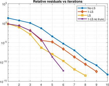
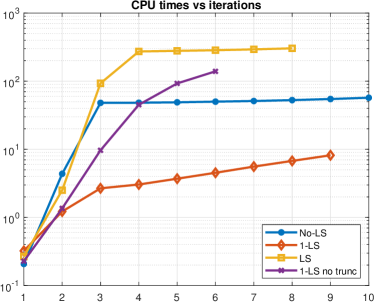
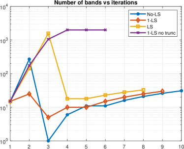
Figure 4: Comparison of the methods in terms of the influence of the line search method and truncation strategy, for $n=2000$.

The performances of the four methods are displayed in Figure 4. The top-left panel shows the beneficial effect of the line search at the first iteration, as it reduces the first residual by an order of magnitude. Among the algorithms that make use of truncation, the LS method exhibits a faster decrease of the residual norm, converging in 8 iterations compared to the 9 and 10 iterations required by 1-LS and No-LS, respectively. However, the LS method necessitates about $400$ seconds to converge, making it slower than the No-LS and 1-LS methods. The fastest method is the 1-LS, which benefits from the initial residual reduction and the low bandwidth of its iterates. The bottom panel of Figure 4 indicates that the high computational cost of LS and No-LS is due to a significant increase of the number of bands during the first iterations, whereas the 1-LS always maintains a bandwidth lower than $40$.

Finally, we compare the performances of the truncated and non-truncated versions of 1-LS. During the initial iterations, the residuals are similar, but ultimately, the 1-LS no trunc achieves a faster reduction and converges in 6 iterations. However, this comes at the price of considering much more bands and consuming much more CPU times, with the latter being an order of magnitude higher than that of the 1-LS case.

In view of the experimental results of this section, for subsequent numerical tests, we will consistently employ the 1-LS version of the tink algorithm.

3.2.2 Comparing tink and d&c_care

We conclude this section by comparing the performances of tink with the divide-and-conquer approach in Algorithm 2. We consider a case study where we vary two parameters: the size $n$ of the matrices and the condition number of the quadratic coefficient $F$. More specifically, we set $A=A_{0}$, $F$ diagonal with entries logarithmically spaced in $\left[\frac{1}{\sqrt{\kappa(F)}},\sqrt{\kappa(F)}\right]$, and $Q=\mathrm{tridiag}(0.1\cdot e,e,0.1\cdot e)$. Then, we solve the CARE with the two algorithms for $n=500\cdot 2^{h}$, $h=0,\dots,4$, and $\kappa(F)\in\{1,10,100,1000\}$. In the case $\kappa(F)=1$, i.e. $F=I$, the tink algorithm uses the conjugate gradient method in place of GMRES.

In Table 2, we report the timings and either the bandwidth or the HSS rank of the computed approximate solution. For each choice of $n$, and $\kappa(F)$, we mark in bold the best CPU time among the two algorithms. In all cases, and for both algorithms, we get relative residuals of the order of $10^{-10}$, so we did not report this data. Note that, the bandwidth of the computed solution grows as $\kappa(F)$ increases; although this growth appears not dramatic on the returned solution, we highlight that the intermediate quantities generated within the Newton-Kleinman iterations have significantly larger bandwidths. This causes the anomalous increase of the CPU time of tink in the case $n=8000$, $\kappa(F)=1000$. Empirically, we have observed that forcing the number of bandwidths to not exceed a prescribed amount (e.g., $150$) in all the intermediate quantities ruins the convergence rate of the Newton’s iteration, resulting in even higher computational times. On the opposite, the HSS rank of the approximate solution and the convergence of EKSM employed in Algorithm 2 are not significantly affected by $\kappa(F)$. As a result, the timings of Algorithm 2 are very similar when fixing $n$. By looking at the numerical results in Table 2, we conclude that tink can compete with d&c_care for small values of $\kappa(F)$, say $\kappa(F)\leq 100$. For poorly conditioned quadratic coefficients, the structure appears to be present in the solution but is less evident, or even absent, in the intermediate terms produced by the Newton-Kleinman scheme. In the latter case one might look for alternative sparsity preserving strategies to limit the bandwidth of intermediate quantities while keeping under control the number of iterations of the method.

Table 2: Comparison of the performances of Algorithm 2, and Algorithm 3, when solving the CAREs considered in Section 3.2.2

Performances of tink (Algorithm 3)
	$\kappa(F)=1$		$\kappa(F)=10$		$\kappa(F)=100$		$\kappa(F)=1000$
$n$	Time	bandwidth	Time	bandwidth	Time	bandwidth	Time	bandwidth
$500$	$\bf 0.4$	$25$	$\bf 0.6$	$30$	$\bf 1.1$	$40$	$3.4$	$50$
$1{,}000$	$\bf 0.7$	$25$	$\bf 1.2$	$30$	$\bf 2.4$	$40$	$3.6$	$50$
$2{,}000$	$\bf 1.6$	$25$	$\bf 2.4$	$30$	$\bf 4.6$	$40$	$8.1$	$50$
$4{,}000$	$\bf 2.7$	$25$	$\bf 5.6$	$30$	$10.8$	$40$	$22.1$	$55$
$8{,}000$	$\bf 5.6$	$25$	$\bf 13.6$	$30$	$25.6$	$40$	$157.8$	$55$

Performances of d&c_care (Algorithm 2)
	$\kappa(F)=1$		$\kappa(F)=10$		$\kappa(F)=100$		$\kappa(F)=1000$
$n$	Time	HSS rank	Time	HSS rank	Time	HSS rank	Time	HSS rank
$500$	$1.6$	$2.42\cdot 10^{-10}$	$1.1$	$7$	$1.2$	$7$	$\bf 1.2$	$7$
$1{,}000$	$2.5$	$1.71\cdot 10^{-10}$	$2.3$	$14$	$\bf 2.4$	$14$	$\bf 2.4$	$14$
$2{,}000$	$4.9$	$1.56\cdot 10^{-10}$	$4.9$	$14$	$4.9$	$14$	$\bf 5.0$	$14$
$4{,}000$	$9.7$	$1.71\cdot 10^{-10}$	$10.0$	$14$	$\bf 10.6$	$14$	$\bf 10.3$	$14$
$8{,}000$	$20.8$	$1.75\cdot 10^{-10}$	$21.6$	$14$	$\bf 22.0$	$14$	$\bf 22.2$	$14$

4 Numerical tests on feedback control applications

This section illustrates the application of the proposed algorithms to the optimal control problems introduced in Section 1.1. In the first numerical experiment, we address the optimal control of a nonlinear PDE, specifically the Allen-Cahn equation. In the second experiment, we focus on the control of a system of interacting particles governed by the Cucker-Smale model.

4.1 Allen-Cahn equation

Let us consider the following nonlinear Allen-Cahn PDE with homogeneous Neumann boundary conditions:

$$\left\{\begin{array}[]{l}\partial_{t}y(t,x)=\sigma\partial_{xx}y(t,x)+y(t,x)(1-y(t,x)^{2})+u(t,x),\\ y(0,x)=y_{0}(x),\end{array}\right.$$

with $x\in[-L,L]$ and $t\in(0,+\infty)$ and the following cost functional

$$\widetilde{J}_{y_{0}}(u)=\int_{0}^{\infty}dt\int_{-L}^{L}dx\;(|y(t,x)|^{2}+\widetilde{\gamma}|u(t,x)|^{2}).$$

Approximating the PDE by finite difference schemes with stepsize $\Delta x$, we obtain the ODEs system in form

$$\dot{y}(s)=A(y)y(s)+Bu(s),$$

and the discretized cost functional reads

$$J_{y_{0}}(u)=\int_{0}^{\infty}\Delta x\,y(t)^{\top}y(t)+\gamma\,u(t)^{\top}u(t)\,dt\,,$$

with

$$A(y)=\sigma A^{\Delta x}_{0}+I_{n}-diag(y\odot y),\quad y\in\mathbb{R}^{n},\quad B=I_{n},$$

where $\odot$ refers to the Hadamard product, $I_{n}\in\mathbb{R}^{n\times n}$ is the identity matrix, $\gamma=\widetilde{\gamma}\Delta x$ and $A^{\Delta x}_{0}$ is the tridiagonal matrix arising from the discretization of the Laplacian with Neumann boundary conditions with stepsize $\Delta x$. We fix $\widetilde{\gamma}=0.1$, $\sigma=10^{-3}$ and $y_{0}=[\sin(\pi x_{i})]_{i=1}^{n}$, with $x_{i}=-L+(i-1)\Delta x$.

The feedback control (2) is derived through solving the SDREs (3), as described in Section 1.1, during the time integration of the dynamical system. Specifically, the system is integrated using the Matlab function ode15s, which is designed for stiff differential equations.

For this numerical test, we employ the tink algorithm to carry on the SDRE approach. Since the closed loop matrix $A(x)-\gamma^{-1}X(x)$ is symmetric for all $x\in\mathbb{R}^{n}$, the linear system (20) arising from the the Newton-Kleinman iterations is solved with the Conjugate Gradient method.

Note that, the exact solution of the SDRE (3) for a given $x\in\mathbb{R}^{d}$ is given by formula (9) with a rescaling term:

$$X(x)=\gamma\left(\sqrt{A(x)^{2}+\gamma^{-1}Q}+A(x)\right).$$ (27)

So, as competitor, we consider the evaluation of formula (27) in dense arithmetic, where the matrix square root is computed using the Matlab function sqrtm.

In Table 3, we compare the performances of the tink algorithm with the use of the exact formula (27) labeled with "sqrtm". The term "CPU per control" denotes the average time required to compute a feedback control as described by (2), specifically for the resolution of an SDRE. The term "Average bandwidth" refers to the average number of diagonals in the approximate solution of the SDREs.

The tink algorithm exhibits an increasing gain with respect to sqrtm as $n$ rises, achieving a speed-up factor of nearly 16 when $n=2000$; this is due to the exceptionally low average bandwidth. Concurrently, we get the same total costs up to the reported digits.

Finally, in Figure 5, we present the time evolution of the uncontrolled dynamics (left panel) and the controlled dynamics using the SDRE solved with tink (right panel) for $n=500$. Observe that the uncontrolled solution converges to a stable equilibrium, with values of 1 when the initial condition is positive and -1 otherwise. Conversely, the SDRE control successfully drives the solution to the unstable equilibrium $\overline{y}=0$ within the initial time instances. The solution controlled via the exact formula closely resembles the one depicted in the left panel of Figure 5 and is therefore not shown.

	tink			sqrtm
$n$	CPU per control	Total cost	Average bandwidth	CPU per control	Total cost
500	0.0108	10.386514	3	0.0261	10.386514
1000	0.0234	10.386514	3	0.1855	10.386514
2000	0.0807	10.386514	8	1.3373	10.386514

Table 3: Comparison of the performances in the computation of the optimal control via tink algorithm and via the exact formula (27) for different dimensions $n$.

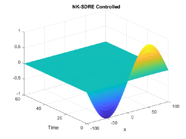
Figure 5: Uncontrolled solution (left) and controlled solution via SDRE solved with tink (right) with $n=500$.

4.2 Cucker-Smale model

Given $N_{a}$ interacting agents, we consider the dynamical system governed by the Cucker-Smale model as follows:

$$\begin{bmatrix}\dot{y}\\ \dot{v}\end{bmatrix}=A(y)\begin{bmatrix}y\\ v\end{bmatrix}+Bu=\begin{bmatrix}0_{N_{a}}&I_{N_{a}}\\ 0_{N_{a}}&\mathcal{A}_{N_{a}}(y)\end{bmatrix}\begin{bmatrix}y\\ v\end{bmatrix}+\begin{bmatrix}O_{N_{a}}\\ I_{N_{a}}\end{bmatrix}u,$$

with the interaction matrix defined by

$$\left[\mathcal{A}_{N_{a}}(y)\right]_{i,j}=\begin{cases}-\frac{1}{N_{a}}\sum_{k\neq i}K(y_{i},y_{k})&if\;i=j,\\ \frac{1}{N_{a}}K(y_{i},y_{j})&otherwise,\end{cases}$$

where

$$K(y_{i},y_{j})=\frac{1}{1+|y_{i}-y_{j}|^{2}}\,.$$

Let $y_{v}=[y;v]\in\mathbb{R}^{n}$, with $n=2N_{a}$. Our objective is to drive all positions and velocities to zero, while minimizing the following cost functional:

$$J(y(\cdot),v(\cdot),u(\cdot))=\int_{0}^{\infty}y(s)^{\top}Q_{N_{a}}y(s)+v(s)^{\top}Q_{N_{a}}v(s)+u(s)^{\top}Ru(s)\,ds,$$

where $Q_{N_{a}}=R=\frac{1}{N_{a}}I_{N_{a}}\in\mathbb{R}^{N_{a}\times N_{a}}$. Due to the block structure of the problem, we consider the solution of the SDRE (3) in block form, $i.e.$,

$$X(y_{v})=\begin{bmatrix}X_{1,1}(y_{v})&X_{1,2}(y_{v})\\ X_{2,1}(y_{v})&X_{2,2}(y_{v})\end{bmatrix}.$$

The SDRE is then equivalent to solving the following system of matrix equations:

$$\begin{cases}-X_{1,2}(y_{v})R^{-1}X_{2,1}(y_{v})+Q_{N_{a}}=0_{N_{a}},\\ X_{1,1}(y_{v})+\mathcal{A}_{N_{a}}(y)X_{1,2}(y_{v})-X_{1,2}(y_{v})R^{-1}X_{2,2}(y_{v})=0_{N_{a}},\\ X_{1,2}(y_{v})+X_{2,1}(y_{v})+\mathcal{A}_{N_{a}}(y)X_{2,2}(y_{v})+X_{1,2}(y_{v})\mathcal{A}_{N_{a}}(y_{v})-X_{2,2}(y_{v})R^{-1}X_{2,2}(y_{v})+Q_{N_{a}}=0_{N_{a}},\\ X_{1,2}(y_{v})=X_{2,1}(y_{v}).\end{cases}$$

We immediately observe that since $R$ is a constant identity matrix, the solution to the first equation is

$$X_{1,2}(y_{v})=X_{2,1}(y_{v})=\sqrt{RQ_{N_{a}}}=\frac{1}{N_{a}}I_{N_{a}}.$$

Substituting this solution into the third equation yields the following SDRE for the block $X_{2,2}(y_{v})$:

$$\mathcal{A}_{N_{a}}(y)X_{2,2}(y_{v})+X_{2,2}(y_{v})\mathcal{A}_{N_{a}}(y)-X_{2,2}(y_{v})R^{-1}X_{2,2}(y_{v})+\frac{3}{N_{a}}I_{N_{a}}=0_{N_{a}}.$$ (28)

For the purpose of implementing the feedback control law (2), we note that the computation of the block $X_{1,1}(y_{v})$ is unnecessary, since the control is given by

$$u(y_{v})=-R^{-1}B^{\top}X(y_{v})y_{v}=-y-R^{-1}X_{2,2}(y_{v})v.$$

The optimal control problem is ultimately reduced to approximating the SDRE (28), where the matrix $\mathcal{A}_{N_{a}}(y)$ exhibits a quasiseparable structure, and both the constant term and the quadratic coefficient are given by constant identity matrices. To ensure an off-diagonal decay of the matrix $\mathcal{A}_{N_{a}}$, we first sort the position variables. Subsequently, we solve the corresponding SDRE (28) and compute the associated feedback law. The control vector is then reordered to match the original configuration of the positions.

For each test, we consider a random initial condition $y_{v}(0)\in\mathbb{R}^{n}$, where each entry lies within the interval $[0,1]$. In Table 4, we compare the performance of the d&c_care algorithm both with and without the inclusion of the aforementioned sorting procedure. In line with the previous numerical test, the term "CPU per control" refers to the average time required to compute a feedback control, specifically for solving the SDRE. Meanwhile, "Average HSS rank" denotes the mean HSS rank of the SDRE solutions throughout the integration process. We observe that incorporating the sorting procedure results in a reduction of the average HSS rank, which consequently decreases CPU time. This effect is illustrated more clearly in Figure 6, where the HSS ranks of the solution to the SDRE at different time instances are depicted. It is noteworthy that the sorted technique begins with a rank of 3, which decreases to 2 after time 5. In contrast, the absence of the initial sorting leads to a rank of 6, which diminishes over the course of time integration. Finally, we emphasize that the CPU time per control scales linearly, making this approach both efficient and scalable for solving high-dimensional problems.

With $n=500$ fixed, Figure 7 illustrates the evolution of the position variables (left panel) and velocity variables (right panel) for the uncontrolled dynamics. It is observed that the velocities reach consensus, converging to a value close to the average of the initial velocities (approximately 0.5325). Due to the presence of positive velocities, the positions increase over time. Conversely, Figure 8 depicts the behaviour of the position and velocity variables under the controlled dynamics. Here, both variables converge to zero, providing a close approximation of the optimal control solution.

	d&c_care with sorting		d&c_care without sorting
$n$	CPU per control	Average HSS rank	CPU per control	Average HSS rank
500	0.1678	2.54	0.1704	3.94
1000	0.4172	2.55	0.4587	3.96
2000	0.7440	2.53	0.9812	3.95

Table 4: Performances in the computation of the optimal control via d&c_care algorithm with and without ordering the position variables for different dimensions $n$.

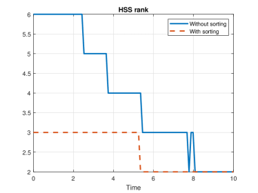
Figure 6: The HSS ranks of the solution to the SDRE (28) at various time instances for both the sorted and unsorted algorithms with $n=2000$.

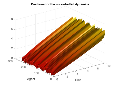
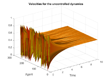
Figure 7: Uncontrolled solution for the positions (left) and for the velocity (right) with $n=500$.

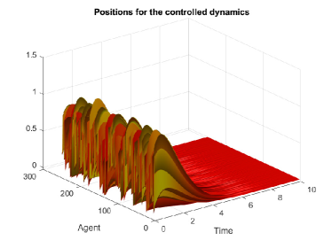
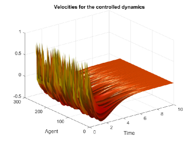
Figure 8: Controlled solution for the positions (left) and for the velocity (right) via SDRE solved with d&c_care with $n=500$.

5 Concluding remarks

In this paper, we have demonstrated that under reasonable assumptions for control problems, continuous-time Riccati equations with quasiseparable coefficients have numerically quasiseparable solutions. Our decay bounds establish a connection between the off-diagonal singular values and Zolotarev numbers, which are linked either to the set $\mathcal{W}(L^{-1}AL)$ or to the spectra of the closed-loop matrices associated with the principal submatrices of the Hamiltonian. Additionally, our analysis provides enhanced estimates for the tensor train ranks of the value function corresponding to the CARE solutions.

Building on this theoretical framework, we have introduced practical methodologies to reduce the computational complexity of solving CAREs with large-scale quasiseparable coefficients. Specifically, we proposed two algorithms: one designed for general quasiseparable coefficients and another tailored for banded coefficients. Numerical experiments validate the scalability of these methods across both synthetic and real-world scenarios, particularly in control theory applications involving partial differential equations and agent-based models.

We remark that there are a few points that might deserve further investigations. First, with additional assumptions the parameter $t$ in the bound of Theorem 2.4 might be improved by following the ideas in Remark 1, and Remark 2, and this would automatically improve the decay bounds given in the corollaries of this result. Second, our bounds ensure the quasiseparable structure of the solution when $F$ is low-rank (apply Theorem 2.3 as in the proof of Theorem 2.10) or when $F$ is full rank (Corollary 2.8, and Corollary 2.9); however, it seems that the solution inherits the structure also in an intermediate scenario where $F$ is rank deficient but not low-rank. In addition, according to the numerical results in Figure 2, the role of $\kappa(F)$ in our upper bounds seems to be an artefact of our proof. Lastly, while testing of the tink algorithm for the banded case, we observed instances where the truncated Newton-Kleinman iteration exhibited a transient phase with large bandwidths, even though the sought solution was approximately banded. It would be of interest to explore whether alternative thresholding techniques could restore computational efficiency in such cases.

References

- [1] A. Alla, D. Kalise, and V. Simoncini. State-dependent Riccati equation feedback stabilization for nonlinear PDEs. Adv. Comput. Math., 49(1):32, 2023. Id/No 9.
- [2] B. D. Anderson and J. B. Moore. Optimal control: linear quadratic methods. Courier Corporation, 2007.
- [3] R. Bailo, M. Bongini, J. A. Carrillo, and D. Kalise. Optimal consensus control of the cucker-smale model. IFAC-PapersOnLine, 51(13):1–6, 2018.
- [4] H. T. Banks, B. M. Lewis, and H. T. Tran. Nonlinear feedback controllers and compensators: a state-dependent Riccati equation approach. Computational Optimization and Applications, 37(2):177–218, 2007.
- [5] M. Bardi, I. C. Dolcetta, et al. Optimal control and viscosity solutions of Hamilton-Jacobi-Bellman equations, volume 12. Springer, 1997.
- [6] B. Beckermann, S. A. Goreinov, and E. E. Tyrtyshnikov. Some remarks on the Elman estimate for GMRES. SIAM J. Matrix Anal. Appl., 27(3):772–778, 2006.
- [7] B. Beckermann and A. Townsend. On the singular values of matrices with displacement structure. SIAM J. Matrix Anal. Appl., 38(4):1227–1248, 2017.
- [8] P. Benner. System-theoretic methods for model reduction of large-scale systems: Simulation, control, and inverse problems. In Proceedings of MATHMOD, volume 2009, pages 126–145. Vienna, Austria: ARGESIM, 2009.
- [9] P. Benner, M. Bollhöfer, D. Kressner, C. Mehl, and T. Stykel. Numerical algebra, matrix theory, differential-algebraic equations and control theory. Switzerland: Springer International Publishing, 2015.
- [10] P. Benner, Z. Bujanović, P. Kürschner, and J. Saak. RADI: a low-rank ADI-type algorithm for large scale algebraic Riccati equations. Numer. Math., 138(2):301–330, 2018.
- [11] P. Benner, Z. Bujanović, P. Kürschner, and J. Saak. A numerical comparison of different solvers for large-scale, continuous-time algebraic Riccati equations and LQR problems. SIAM J. Sci. Comput., 42(2):A957–A996, 2020.
- [12] P. Benner, M. Heinkenschloss, J. Saak, and H. K. Weichelt. An inexact low-rank Newton–ADI method for large-scale algebraic Riccati equations. Applied Numerical Mathematics, 108:125–142, 2016.
- [13] M. Benzi, P. Boito, and N. Razouk. Decay properties of spectral projectors with applications to electronic structure. SIAM Rev., 55(1):3–64, 2013.
- [14] D. A. Bini, B. Iannazzo, and B. Meini. Numerical solution of algebraic Riccati equations. SIAM, 2011.
- [15] T. Breiten and K. Kunisch. Feedback stabilization of the schlögl model by lqg-balanced truncation. In 2015 European Control Conference (ECC), pages 1171–1176. IEEE, 2015.
- [16] T. Çimen. State-dependent riccati equation (SDRE) control: a survey. IFAC Proceedings Volumes, 41(2):3761–3775, 2008.
- [17] M. Crouzeix and C. Palencia. The numerical range is a -spectral set. SIAM J. Matrix Anal. Appl., 38(2):649–655, 2017.
- [18] F. Cucker and S. Smale. Emergent behavior in flocks. IEEE Transactions on automatic control, 52(5):852–862, 2007.
- [19] S. Dolgov, D. Kalise, and K. K. Kunisch. Tensor decomposition methods for high-dimensional Hamilton-Jacobi-Bellman equations. SIAM J. Sci. Comput., 43(3):A1625–A1650, 2021.
- [20] S. Dolgov, D. Kalise, and L. Saluzzi. Data-driven tensor train gradient cross approximation for Hamilton-Jacobi-Bellman equations. SIAM J. Sci. Comput., 45(5):a2153–a2184, 2023.
- [21] S. Dolgov and B. Khoromskij. Two-level QTT-Tucker format for optimized tensor calculus. SIAM J. Matrix Anal. Appl., 34(2):593–623, 2013.
- [22] T. A. Driscoll, N. Hale, and L. N. Trefethen. Chebfun guide, 2014.
- [23] Y. Eidelman, I. Gohberg, and I. Haimovici. Separable type representations of matrices and fast algorithms. Vol. 1, volume 234 of Operator Theory: Advances and Applications. Birkhäuser/Springer, Basel, 2014. Basics. Completion problems. Multiplication and inversion algorithms.
- [24] H. C. Elman. Iterative methods for large, sparse, nonsymmetric systems of linear equations. Yale University, 1982.
- [25] M. Embree. Extending elman’s bound for gmres. arXiv preprint arXiv:2312.15022, 2023.
- [26] F. Feitzinger, T. Hylla, and E. W. Sachs. Inexact Kleinman–Newton method for Riccati equations. SIAM Journal on Matrix Analysis and Applications, 31(2):272–288, 2009.
- [27] E. S. Gawlik. Zolotarev iterations for the matrix square root. SIAM J. Matrix Anal. Appl., 40(2):696–719, 2019.
- [28] L. Grasedyck. Nonlinear multigrid for the solution of large-scale Riccati equations in low-rank and -matrix format. Numer. Linear Algebra Appl., 15(9):779–807, 2008.
- [29] L. Grasedyck, W. Hackbusch, and B. N. Khoromskij. Solution of large scale algebraic matrix Riccati equations by use of hierarchical matrices. Computing, 70(2):121–165, 2003.
- [30] A. Haber and M. Verhaegen. Sparsity preserving optimal control of discretized PDE systems. Comput. Methods Appl. Mech. Eng., 335:610–630, 2018.
- [31] W. Hackbusch. Hierarchical matrices: algorithms and analysis, volume 49 of Springer Series in Computational Mathematics. Springer, Heidelberg, 2015.
- [32] D. Halikias and A. Townsend. Structured matrix recovery from matrix-vector products. Numerical Linear Algebra with Applications, 31(1):e2531, 2024.
- [33] N. Halko, P.-G. Martinsson, and J. A. Tropp. Finding structure with randomness: Probabilistic algorithms for constructing approximate matrix decompositions. SIAM review, 53(2):217–288, 2011.
- [34] V. Kazeev, O. Reichmann, and C. Schwab. Low-rank tensor structure of linear diffusion operators in the TT and QTT formats. Linear Algebra Appl., 438(11):4204–4221, 2013.
- [35] D. Kleinman. On an iterative technique for Riccati equation computations. IEEE Transactions on Automatic Control, 13(1):114–115, 1968.
- [36] D. Kressner, P. Kürschner, and S. Massei. Low-rank updates and divide-and-conquer methods for quadratic matrix equations. Numer. Algorithms, 84(2):717–741, 2020.
- [37] D. Kressner, S. Massei, and L. Robol. Low-rank updates and a divide-and-conquer method for linear matrix equations. SIAM J. Sci. Comput., 41(2):A848–A876, 2019.
- [38] D. Kressner, S. Massei, and J. Zhu. Improved ParaDiag via low-rank updates and interpolation. Numer. Math., 155(1-2):175–209, 2023.
- [39] P. Lancaster and L. Rodman. Algebraic Riccati equations. Oxford: Clarendon Press, 1995.
- [40] J. Levitt and P.-G. Martinsson. Linear-complexity black-box randomized compression of rank-structured matrices. SIAM Journal on Scientific Computing, 46(3):A1747–A1763, 2024.
- [41] S. Massei, D. Palitta, and L. Robol. Solving rank-structured Sylvester and Lyapunov equations. SIAM J. Matrix Anal. Appl., 39(4):1564–1590, 2018.
- [42] S. Massei, L. Robol, and D. Kressner. hm-toolbox: MATLAB software for HODLR and HSS matrices. SIAM J. Sci. Comput., 42(2):C43–C68, 2020.
- [43] A. Melman. Generalization and variations of Pellet’s theorem for matrix polynomials. Linear algebra and its applications, 439(5):1550–1567, 2013.
- [44] I. V. Oseledets. Tensor-train decomposition. SIAM J. Sci. Comput., 33(5):2295–2317, 2011.
- [45] I. V. Oseledets. Constructive representation of functions in low-rank tensor formats. Constr. Approx., 37(1):1–18, 2013.
- [46] J. R. Silvester. Determinants of block matrices. The Mathematical Gazette, 84(501):460–467, 2000.
- [47] V. Sima. Algorithms for linear-quadratic optimization, volume 200 of Pure Appl. Math., Marcel Dekker. New York, NY: Marcel Dekker, 1996.
- [48] V. Simoncini. A new iterative method for solving large-scale Lyapunov matrix equations. SIAM J. Sci. Comput., 29(3):1268–1288, 2007.
- [49] V. Simoncini. Analysis of the rational Krylov subspace projection method for large-scale algebraic Riccati equations. SIAM J. Matrix Anal. Appl., 37(4):1655–1674, 2016.
- [50] V. Simoncini. Computational methods for linear matrix equations. SIAM Rev., 58(3):377–441, 2016.
- [51] V. Simoncini, D. B. Szyld, and M. Monsalve. On two numerical methods for the solution of large-scale algebraic Riccati equations. IMA J. Numer. Anal., 34(3):904–920, 2014.
- [52] A. Townsend and H. Wilber. On the singular values of matrices with high displacement rank. Linear Algebra Appl., 548:19–41, 2018.
- [53] R. Vandebril, M. Van Barel, and N. Mastronardi. Matrix computations and semiseparable matrices. Vol. 1. Johns Hopkins University Press, Baltimore, MD, 2008. Linear systems.
- [54] J. Xia. On the complexity of some hierarchical structured matrix algorithms. SIAM Journal on Matrix Analysis and Applications, 33(2):388–410, 2012.
- [55] J. Xia, S. Chandrasekaran, M. Gu, and X. S. Li. Fast algorithms for hierarchically semiseparable matrices. Numer. Linear Algebra Appl., 17(6):953–976, 2010.