Tight bound on neutron-star radius with quasiperiodic oscillations in short gamma-ray bursts

Abstract

Quasiperiodic oscillations (QPOs) have been recently discovered in the short gamma-ray bursts (GRBs) 910711 and 931101B. Their frequencies are consistent with those of the radial and quadrupolar oscillations of binary neutron star merger remnants, as obtained in numerical relativity simulations. These simulations reveal quasiuniversal relations between the remnant oscillation frequencies and the tidal coupling constant of the binaries. Under the assumption that the observed QPOs are due to these postmerger oscillations, we use the frequency-tide relations in a Bayesian framework to infer the source redshift, as well as the chirp mass and the binary tidal deformability of the binary neutron star progenitors for GRBs 910711 and 931101B. We further use this inference to estimate bounds on the mass-radius relation for neutron stars. By combining the estimates from the two GRBs, we find a 68% credible range $R_{1.4}=12.48^{+0.41}_{-0.41}$ km for the radius of a neutron star with mass $M=1.4$ M_⊙, which is one of the tightest bounds to date.

1 Introduction

Recent measurements of neutron-star (NS) radii through X-ray observations (Miller et al., 2019, 2021; Riley et al., 2019, 2021; Dittmann et al., 2024; Salmi et al., 2024; Choudhury et al., 2024) have established significant constraints on the equation of state (EOS) for these objects, a long-standing problem in nuclear astrophysics. In addition, gravitational-wave (GW) observations from a binary neutron star (BNS) merger, GW170817 (Abbott et al., 2017a), and the concurrent detection of a short gamma-ray burst (GRB), GW170817A (Abbott et al., 2017b), revolutionized multimessenger astronomy, constraining the EOS through measurements of the binary tidal deformability (Abbott et al., 2018a; De et al., 2018) and strengthening the hypothesis that BNS mergers are sources of short GRBs.

More recently, kilohertz quasiperiodic oscillations (QPOs) were found in the light curves of GRBs 910711 and 931101B (Chirenti et al., 2023), raising the possibility that some short GRBs can exhibit sub-millisecond variability originating from the short GRB central engine. The central engines of short GRBs are required to launch a highly relativistic outflow, with postmerger BNSs being strong candidates, given the high energy and the rapid variability of the prompt emission (Nakar, 2007; Berger, 2014). Generally, the outcome of a BNS merger depends on the binary mass and on the EOS (see Sarin & Lasky, 2021, for a recent review). For example, low-mass BNSs can produce a stable NS remnant, while higher mass binaries can result in the promt collapse to a black hole. Most relevant to our work, hypermassive neutron stars (HMNSs) are possible BNS merger remnants that are briefly supported against collapse to a black hole by differential rotation (Baumgarte et al., 2000), lasting for only tens to hundreds of milliseconds, depending on how the stability of these objects is affected by thermal and magnetic processes after the merger (Radice et al., 2020).

Although a black hole central engine has been favored in the literature, the nature of the central engine and the necessary conditions for the successful launching and breakthrough of the jet are still under debate (D’Avanzo, 2015; Ciolfi, 2018). For instance, Murguia-Berthier et al. (2014) suggests that the merger remnant must collapse within $\sim$ 100 ms, otherwise the jet is choked by the neutrino-driven wind from the remnant, thus supporting the prompt collapse and short-lived ($\lesssim 20$ ms) remnant scenarios. Nevertheless, observations of X-ray afterglows in short GRBs provide evidence that long-lived ($\gtrsim 20$ ms) remnants can produce the prompt emission and therefore power the afterglow (Lü et al., 2015) and this scenario is also supported by recent numerical relativity (NR) simulations (Mösta et al., 2020).

The QPOs reported by Chirenti et al. (2023) have frequencies that can be interpreted as oscillation modes of the HMNS. GRBs 910711 and 931101B show two QPOs each, with similar centroid frequencies for both GRBs: a lower frequency QPO at $\sim 1$ kHz and a higher frequency QPO at $\sim 2.6$ kHz (see Table 1). NR simulations have shown that these BNS merger remnants have a rich GW spectrum, with peaks in the range $\sim$ 1 $-$ 5 kHz (Bauswein & Janka, 2012; Takami et al., 2015). The main peaks in the GW spectrum are characterized by the frequencies $f_{2}$ and $f_{2}\pm f_{0}$ (Rezzolla & Takami, 2016), where $f_{2}$ is the frequency of the quadrupolar ($\ell=2$) mode, in the range $\sim$ 1 $-$ 4 kHz, and $f_{0}$ is the frequency of the radial ($\ell=0$) mode, around $\sim$ 1 kHz. We note that the frequencies of the QPOs reported in Chirenti et al. (2023) are in good agreement with these quadrupolar and radial oscillation modes, thus supporting such an interpretation. If this correspondence holds, it is possible that the jet would have to be launched shortly after the merger, otherwise the modes would have been damped away due to the emission of GWs (Bernuzzi et al., 2016) and the modulation of the GRB signal would not be statistically significant (Chirenti et al., 2019). This suggests that the prompt emission should happen in the HMNS phase (see Curtis et al., 2024).

The oscillation modes of short-lived or long-lived postmerger remnants have been shown to follow quasiuniversal relations (i.e., relations that exhibit a weak dependence on the EOS) with premerger parameters such as the binary tidal deformability (Breschi et al., 2019; Lioutas et al., 2021; Gonzalez et al., 2023). These modes should be observed in the postmerger GW signal and their detection is expected to place tight bounds on NS radii and strong constraints on the EOS (Chatziioannou et al., 2024). Signatures of BNS postmerger remnants are still to be observed in GWs due to the lack of sensitivity of current detectors in the kilohertz range (Abbott et al., 2018b), a scenario that is expected to change with third generation detectors (Punturo et al., 2010; Reitze et al., 2019). Short GRBs, on the other hand, are detected $\sim$ weekly and the possibility that at least a fraction of these signals is modulated by the GW frequencies of the central engine brings a novel way to obtain information about the EOS of NS matter.

In this work, we assume that the frequencies of the two QPOs observed in both GRB 910711 and GRB 191101B correspond to the frequencies of the quadrupolar mode $f_{2}$ and radial mode $f_{0}$ from BNS simulations. Given this assumption, we obtain constraints on the redshift of the GRBs, as well as the binary tidal deformability and the chirp mass of the corresponding BNS merger event; we further estimate the radius of a 1.4 M_⊙ NS and obtain a constraint on the mass-radius diagram.

2 Methods and Results

2.1 Observations

We analyze GRBs 910711 and 931101B separately. For each one, there are two measurements for the QPOs: $\nu_{1}\pm\sigma_{\nu_{1}}$ and $\nu_{2}\pm\sigma_{\nu_{2}}$, both measured in the detector frame and thus redshifted relative to the source frame. We take the values for $\nu_{1}$ and $\nu_{2}$ from Table 1 of Chirenti et al. (2023), and choose for $\sigma_{\nu_{1}}$ and $\sigma_{\nu_{2}}$ the average of the uncertainties for each measurement (a reasonable approximation since the reported $\pm 1\sigma$ ranges are very similar).

In our analysis, we identify these QPOs observed in short GRBs with oscillation modes of HMNSs obtained from NR simulations of merging NSs. In short, we associate $\nu_{2}$ with the frequency of the quadrupolar ($\ell=2$) mode $f_{2}$ and $\nu_{1}$ with the radial ($\ell=0$) mode $f_{0}$, both measured in the source frame (see Section 2.2 for more details). In order to keep a consistent notation (with respect to the modes that we are associating $\nu_{1}$ and $\nu_{2}$ with), we rename $\nu_{1}$ as $\nu_{1}\equiv\nu_{0}$. Furthermore, for our purposes, it is more useful to work with $\nu_{2}$ and $\nu_{2}/\nu_{0}\equiv\nu_{02}$, which are our observables. Table 1 shows the measurements that we consider.

GRB	$T_{90}$ [ms]	$\nu_{0}$ [kHz]	$\sigma_{\nu_{0}}$ [kHz]	$\nu_{2}$ [kHz]	$\sigma_{\nu_{2}}$ [kHz]	$\nu_{02}$	$\sigma_{\nu_{02}}$
910711	14	1.113	0.008	2.649	0.007	2.38	0.02
931101B	34	0.877	0.007	2.612	0.009	2.98	0.03

Table 1: The QPO frequencies and associated uncertainties $\nu_{0}\pm\sigma_{\nu_{0}}$ and $\nu_{2}\pm\sigma_{\nu_{2}}$ for the GRBs 910711 and 931101B from Chirenti et al. (2023) (note that those authors use $\nu_{1}\pm\sigma_{\nu_{1}}$ to refer to the lower frequency QPO that, here, is $\nu_{0}\pm\sigma_{\nu_{0}}$). We consider $\nu_{2}$ and the ratio $\nu_{02}\equiv\nu_{2}/\nu_{0}$ as our measurements. We also quote $T_{90}$ for each GRB, which is the time span that contains 90$\%$ of the counts or, roughly, the duration of the GRB (cf. survival time of the remnant in Fig. 1).

2.2 Simulations

For given EOS and mass-ratio $q=M_{1}/M_{2}$ (for $M_{1}\geq M_{2}$), we can label a BNS system by the chirp mass:

$$\mathcal{M}\equiv\frac{(M_{1}M_{2})^{3/5}}{(M_{1}+M_{2})^{1/5}},$$ (1)

or the binary tidal deformability (see, e.g., Lackey & Wade 2015):

$$\tilde{\Lambda}\equiv\frac{16}{13}\left(\frac{(M_{1}+12M_{2})M^{4}_{1}{\bar{\Lambda}}_{1}}{(M_{1}+M_{2})^{5}}+(1\leftrightarrow 2)\right),$$ (2)

where $M_{A}$ and ${\bar{\Lambda}}_{A}\equiv\Lambda_{A}/M^{5}_{A}$ are the mass and dimensionless tidal deformability of the $A^{\rm th}$ NS in the binary. The postmerger phase of BNS merger simulations is characterized by the amplitude of the GW signal $h(t)$ and the central rest-mass density of the postmerger remnant $\rho_{\rm max}(t)$, the latter being relevant in the case of a delayed collapse. The two dominant modes in the postmerger GW spectrum are the $\ell=2$ and $\ell=0$ modes, characterizing the frequencies $f_{2}$ and $f_{0}$. The latter is seen in the GW spectrum in the combination $f_{2}\pm f_{0}$, but can also be extracted directly from the pulsations in the central density of the remnant. Being the lowest order modes, these are the most likely to be imprinted in the electromagnetic counterpart of the GW signal and thus modulate the GRB signal.

We consider a subset of the simulations in Breschi et al. (2019) that report $\rho_{\rm max}$ for short- and long-lived remnants, from which we obtain the frequencies $f_{2}$ and $f_{0}$ by performing a Fourier analysis of $h(t)$ and $\rho_{\rm max}(t)$. For $h(t)$, we apply the Fourier transform between the time of merger, $t_{\rm merger}$ (for definitions, see Breschi et al. 2019), and the final time of the simulation, $t_{\rm final}$. In cases where the apparent horizon is formed within the time of the simulation, we redefine $t_{\rm final}$ for our analysis as the time shortly before when $\rho_{\max}(t)$ drops to zero (this indicates the collapse to a black hole as the region inside the black hole is excluded from the simulation). For the analysis of $\rho_{\rm max}(t)$, we detrend the function between $t_{\rm merger}$ and $t_{\rm final}$ before applying the Fourier transform by finding the best fourth order polynomial fit for $\rho_{\rm max}(t)$ and subtracting it from the function; we further remove the offset of the resulting function with respect to zero. We show in Fig. 1 an example of the Fourier transform for $h(t)$ and $\rho_{\rm max}(t)$, as well as their spectrograms, for a BNS system with $q=1$ ($M_{1}=M_{2}=1.35$ M_⊙) and the piecewise polytropic SLy EOS.

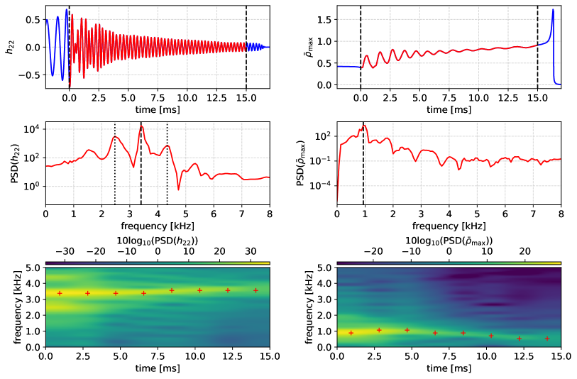
Figure 1: Top: $\ell=m=2$ waveform mode ($h_{22}$) for the postmerger GW signal (left) and the maximum rest-mass density for the postmerger remnant normalized by the maximum stable central density for a nonrotating star with that EOS (${\bar{\rho}}_{\rm max}\equiv\rho_{\rm max}/\rho_{\rm TOV}$) (right) from the merger of two NSs of mass $1.35$ M_⊙ described by the piecewise polytropic approximation to the SLy EOS (Read et al., 2009). The vertical dashed lines indicate the merger time $t_{\rm merger}$ and final time $t_{\rm final}$ within which we perform the Fourier transform. Middle: Power spectral density (PSD) of $h_{22}$ (left) and ${\bar{\rho}}_{\rm max}$ (right) between $t_{\rm merger}$ and $t_{\rm final}$. The vertical dashed lines indicate the peak frequencies in the spectra, $f_{2}$ (left) and $f_{0}$ (right), while the dotted lines in the left panel shows the beat frequencies $f_{2}\pm f_{0}$. Bottom: Spectrogram for $h_{22}$ (left) and ${\bar{\rho}}_{\rm max}$ (right). Note that the frequencies are approximately constant during the time span of the analysis and $f_{0}$ $\rightarrow$ $\approx 0$ as $t$ $\rightarrow$ $\approx t_{\rm final}$ as expected since the remnant collapses to a black hole.

Using the results for $f_{2}$ and $f_{0}$ for a range in $q$ between 1 and $\approx$ 1.66 and given the parameters $\mathcal{M}$ and $\tilde{\Lambda}$ for each binary, we obtain the new quasiuniversal relations (shown in Fig. 2): $f_{2}/f_{0}\equiv f_{02}$ vs. $\tilde{\Lambda}$ and $\mathcal{M}f_{2}\equiv\bar{f}_{2}$ vs. $\tilde{\Lambda}$. Note that $f_{02}$ is independent of the redshift $z$, but $\bar{f}_{2}$ is not. We use a set of eight EOSs; six tabulated models: BHBlp (Banik et al., 2014), BLh (Bombaci & Logoteta, 2018; Typel et al., 2010), DD2 (Typel et al., 2010; Hempel & Schaffner-Bielich, 2010), LS220 (Lattimer & Swesty, 1991), SFHo (Steiner et al., 2013), SLy4 (Douchin & Haensel, 2001); and two piecewise polytropic fits to tabulated models: SLy and MS1b (Read et al., 2009). We construct fits for these quasiuniversal relations with the following fitting function (Breschi et al., 2019):

$$Q^{\rm fit}(\tilde{\Lambda})=Q_{0}\left(\frac{1+n_{1}\tilde{\Lambda}+n_{2}{\tilde{\Lambda}}^{2}}{1+d_{1}\tilde{\Lambda}+d_{2}{\tilde{\Lambda}}^{2}}\right),$$ (3)

where $Q^{\rm fit}$ $\in$ $\{$${\bar{f}}_{2}$, $f_{02}$$\}$ while $Q_{0}$, $n_{i}$, and $d_{i}$ ($i$ $\in$ $\{$1, 2$\}$) are the fitting coefficients. We overlay these fits in Fig. 2 and present the best-fit coefficients as well as different measures for the fit quality in Table 2.

These quasiuniversal relations are slightly different from the ones reported in Breschi et al. (2019): those authors consider the relations ${\hat{f}}_{2}$ vs. $\xi$ and ${\hat{f}}_{2\pm 0}$ vs. $\xi$, where the frequencies ${\hat{f}}_{2}$ and ${\hat{f}}_{2\pm 0}$ are normalized by the binary mass and $\xi$ is defined in terms of the binary tidal polarizability (see the reference for more details). Further, we note that the relations that we propose here could be affected by phase transitions in the EOS and such effects have not been implemented in the set of simulations that we consider. However, we stress that these effects could be degenerate with the spread of the relations if not strong enough (Prakash et al., 2024).

Table 2: Fitting coefficients for the quasiuniversal relations ${\bar{f}}_{2}(\tilde{\Lambda})$ and $f_{02}(\tilde{\Lambda})$, using the fitting function in Eq. (3). We also quote: $\sigma_{Q}$, the standard deviation for the parameters; $\sigma_{r}$, the standard deviation for the relative residues $r\equiv 1-Q^{\rm NR}/Q^{\rm fit}$; the $\chi^{2}$ statistic, $\chi^{2}\equiv\sum^{N}_{i=1}r^{2}_{i}$, where $N$ is the number of data points (i.e., number of simulations for various EOSs and mass-ratios); the Kullback-Leibler divergence, $D_{\rm KL}\equiv\sum^{N}_{i=1}{\mathcal{P}}_{i}{\rm ln}(\mathcal{P}_{i}/\mathcal{Q}_{i})$, between the distribution $\mathcal{P}$ for the relative residuals $r$ and a normal distribution $\mathcal{Q}$ with zero mean and standard deviation $\sigma_{r}$.

$Q$	$Q_{0}$	$n_{1}$	$n_{2}$	$d_{1}$	$d_{2}$	$\sigma_{Q}$	$\sigma_{r}$	$\chi^{2}$	$D_{\rm KL}$
${\bar{f}}_{2}$	1.463	9.930$\times 10^{2}$	7.556$\times 10^{-1}$	1.948$\times 10^{2}$	6.973$\times 10^{-1}$	1.711$\times 10^{-1}$	5.028$\times 10^{-2}$	2.477$\times 10^{-1}$	9.447
$f_{02}$	2.146	5.248$\times 10^{3}$	1.031$\times 10^{1}$	$-$7.873$\times 10^{2}$	1.557$\times 10^{1}$	3.981$\times 10^{-1}$	1.249$\times 10^{-1}$	1.529	1.369

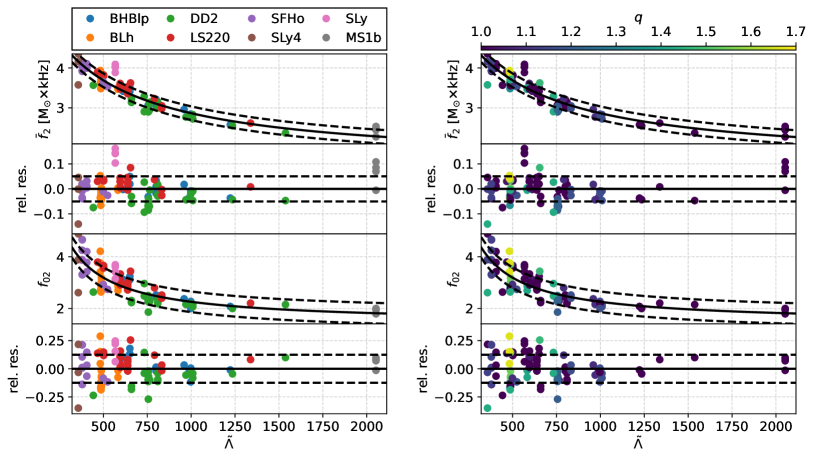
Figure 2: Quasiuniversal relations ${\bar{f}}_{2}(\tilde{\Lambda})$ and $f_{02}(\tilde{\Lambda})$. We show the EOS variation (left, see the different colors) and mass-ratio ($q$) variation (right, see the colorbar) of these relations. The solid lines are the best fits for these relations (using the fitting function in Eq. (3)) and the dashed lines represent the $1\sigma$ ($68.3\%$) credible regions. We also show the relative residues $1-Q^{\rm NR}/Q^{\rm fit}$, where $Q$ $\in$ $\{$${\bar{f}}_{2}$, $f_{02}$$\}$, for these relations and the corresponding 1$\sigma$ credible regions.

2.3 Priors, likelihoods, and posteriors

We use the best fits for the quasiuniversal relations $f_{02}(\tilde{\Lambda})$ and $\bar{f}_{2}(\tilde{\Lambda})$ and their standard deviations $\sigma_{f_{02}}$ and $\sigma_{\bar{f}_{2}}$ (see Table 2), to obtain the joint posterior $P$ on $\tilde{\Lambda}$, $\mathcal{M}$, and $z$, by using the standard Bayesian expression (see, e.g., Miller et al. 2020 for application to EOS inference from NS observations):

$$P(\tilde{\Lambda},\mathcal{M},z)\propto p(\tilde{\Lambda},\mathcal{M},z)\mathcal{L}(\tilde{\Lambda},\mathcal{M},z),$$ (4)

where $p({\tilde{\Lambda}},{\cal M},z)$ is the prior (normalized so that the integral over all values of ${\tilde{\Lambda}}$, ${\cal M}$, and $z$ is unity), ${\cal L}({\tilde{\Lambda}},{\cal M},z)$ is the likelihood of the data given the model, and the proportionality is because the posterior, like the prior, is a probability density and thus must be normalized.

Prior

We decompose the prior as:

$$p(\tilde{\Lambda},\mathcal{M},z)=p(\tilde{\Lambda},\mathcal{M})p(z),$$ (5)

where we take into account the correlation between $\tilde{\Lambda}$ and $\mathcal{M}$ (see, e.g., Zhao & Lattimer 2018) when writing the joint prior on these parameters, i.e.,

$$p(\tilde{\Lambda},\mathcal{M})=p(\tilde{\Lambda})p(\mathcal{M}|\tilde{\Lambda}).$$ (6)

For the range in $\mathcal{M}$ that we consider here ([1.04, 1.31] M_⊙), which is determined by our set of NR simulations, the relation $\mathcal{M}$ $vs.$ $\tilde{\Lambda}$ is approximately linear (with a Pearson correlation coefficient of $\sim$ $-0.5$). We can thus find the best fit $\mathcal{M}(\tilde{\Lambda})=a_{0}+a_{1}\tilde{\Lambda}$ (with $a_{0}=1.332$ M_⊙ and $a_{1}=-2.216\times 10^{-4}$ M_⊙) and corresponding standard deviation ($\sigma_{\mathcal{M}}$ = $7.068\times 10^{-2}$ M_⊙). Then, we can write:

$$p(\mathcal{M}|\tilde{\Lambda})\propto{\rm exp}\left(-\frac{(\mathcal{M}-\mathcal{M}(\tilde{\Lambda}))^{2}}{2\sigma^{2}_{\mathcal{M}}}\right).$$ (7)

We assume $p(\tilde{\Lambda})$ to be uniform in the range informed by the NR simulations ([357, 2053]). We consider $p(z)$ to correspond to the redshift distribution in Guetta & Piran (2005), obtained from the luminosity function determined from the peak flux distribution of short GRBs in the BATSE data. We consider the distribution that takes into account the star formation rate and the merger time delay of BNSs for short GRBs, with a peak in $z\sim 0.5$ (see their Fig. 3), and that agrees with more recent data (see, e.g., Fig. 4 in Berger 2014); we consider the same range for $z$ ([0, 5]).

Likelihood

The likelihood can be written as:

$$\mathcal{L}(\tilde{\Lambda},\mathcal{M},z)=\mathcal{L}_{\nu_{02}}(\tilde{\Lambda})\mathcal{L}_{\nu_{2}}(\tilde{\Lambda},\mathcal{M},z),$$ (8)

where:

$$\mathcal{L}_{\nu_{02}}(\tilde{\Lambda}) \equiv\mathcal{L}(\nu_{02}|f_{02}(\tilde{\Lambda}))\propto{\rm exp}\left(-\frac{(\nu_{02}-f_{02}(\tilde{\Lambda}))^{2}}{2(\sigma^{2}_{\nu_{02}}+\sigma^{2}_{f_{02}})}\right),$$ (9)

$$\mathcal{L}_{\nu_{2}}(\tilde{\Lambda},\mathcal{M},z) \equiv\mathcal{L}(\nu_{2}|f^{\rm obs}_{2}(\tilde{\Lambda},\mathcal{M},z))\propto{\rm exp}\left(-\frac{(\nu_{2}-f^{\rm obs}_{2}(\tilde{\Lambda},\mathcal{M},z))^{2}}{2(\sigma^{2}_{\nu_{2}}+\sigma^{2}_{f^{\rm obs}_{2}}(\mathcal{M},z))}\right),$$ (10)

with the definitions $f^{\rm obs}_{2}(\tilde{\Lambda},\mathcal{M},z)\equiv\bar{f}_{2}(\tilde{\Lambda})/\mathcal{M}(1+z)$ and $\sigma_{f^{\rm obs}_{2}}(\mathcal{M},z)\equiv\sigma_{{\bar{f}}_{2}}/\mathcal{M}(1+z)$. In Eqs. (9) and (10), we sum the standard deviations (from our model and the data) in quadrature because we assume that the uncertainties are uncorrelated with each other.

In Fig. 3, we show the results for the 1D and 2D marginalized posterior probability distributions for the parameters $\tilde{\Lambda}$, $\mathcal{M}$, and $z$ considering the measurements for the two GRBs in Table 1. We summarize the results in the first three columns of Table 3, where we quote the mean and $\pm 1\sigma$ ranges for the parameters. The posterior distributions are very informative, when compared to the prior distributions, with the values of $\tilde{\Lambda}$ and $\mathcal{M}$ being consistent with expected values for BNS mergers, and with the low values of $z$ being consistent with the expectation that GRBs 910711 and 931101B occurred relatively close to us (Chirenti et al., 2023).

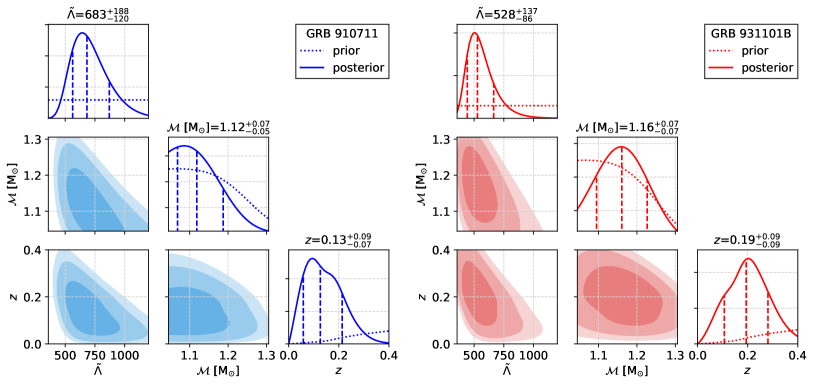
Figure 3: Results for the parameter estimation using the observed QPOs (see Table 1) in GRBs 910711 (left) and 931101B (right), and the quasiuniversal relations ${\bar{f}}_{2}(\tilde{\Lambda})$ and $f_{02}(\tilde{\Lambda})$ (see Fig. 2). Off-Diagonal: 2D marginalized posterior probability distributions for $(\tilde{\Lambda},\mathcal{M})$, $(\mathcal{M},z)$, and $(z,\tilde{\Lambda})$. The three different color tones represent the 1$\sigma$ (68.3$\%$), 2$\sigma$ (95.4$\%$), and 3$\sigma$ (99.7$\%$) credible regions from dark to light. Diagonal: 1D marginalized posterior probability distributions (solid) as well as prior (dotted) for $\tilde{\Lambda}$, $\mathcal{M}$, and $z$. The dashed lines represent the median and the $\pm 1\sigma$ values.

Table 3: Measurement for the binary tidal deformability $\tilde{\Lambda}$, chirp mass $\mathcal{M}$, and redshift $z$ for the GRBs 910711 and 931101B. The values for $\tilde{\Lambda}$ and $\mathcal{M}$ are consistent with expected values for BNS mergers, e.g., $\tilde{\Lambda}=390^{+500}_{-190}$ and $\mathcal{M}=1.118^{+0.001}_{-0.001}$ M_⊙ for GW170817 (Abbott et al., 2019). We also quote the median and $\pm 1\sigma$ ranges for the frequencies of the quadrupolar mode $f_{2}$, radial mode $f_{0}$, and the ratio $f_{02}\equiv f_{2}/f_{0}$, that we determined through the result for $z$.

GRB	$\tilde{\Lambda}$	$\mathcal{M}$ [M⊙]	$z$	$f_{2}$ [kHz]	$f_{0}$ [kHz]	$f_{02}$
910711	683${}^{+188}_{-120}$	1.12${}^{+0.07}_{-0.05}$	0.13${}^{+0.09}_{-0.07}$	$2.99^{+0.24}_{-0.21}$	$1.25^{+0.10}_{-0.09}$	$2.39^{+0.26}_{-0.23}$
931101B	528${}^{+137}_{-86}$	1.16${}^{+0.07}_{-0.07}$	0.19${}^{+0.09}_{-0.09}$	$3.16^{+0.26}_{-0.24}$	$1.06^{+0.08}_{-0.08}$	$2.99^{+0.35}_{-0.31}$

In order to validate our results, we experimented with more conservative ranges for the priors in $\tilde{\Lambda}$ and $\mathcal{M}$ ([300, 5000] and [0.9, 1.4] M_⊙, respectively). The results for the posteriors are consistent with the previous results within the $\pm 1\sigma$ ranges. However, we stress that the extended ranges for the priors rely on the assumption that the quasiuniversal relations, ${\bar{f}}_{2}(\tilde{\Lambda})$ and $f_{02}(\tilde{\Lambda})$ (see Fig. 1), and the correlation between $\mathcal{M}$ and $\tilde{\Lambda}$ can be extrapolated. We also tried using a redshift distribution for short GRBs that does not take into account the delay time for BNS mergers (see Fig. 3 of Guetta & Piran, 2005) as a prior for $z$ and the results are also consistent with Table 3.

2.4 Estimating the source-frame frequencies and constraining the neutron-star mass-radius relation

Based on the measurements for $\tilde{\Lambda}$, $\mathcal{M}$, and $z$, we now determine the source-frame frequencies $f_{\ell}$ ($\ell$ $\in$ $\{$0, 2$\}$), which are:

$$f_{\ell}=f^{\rm obs}_{\ell}(1+z).$$ (11)

From the parameter estimation performed in Section 2.3, we have $P(\tilde{\Lambda},\mathcal{M},z)$, and we can obtain the distribution for the redshift $z$ by marginalizing $P(\tilde{\Lambda},\mathcal{M},z)$ over $\tilde{\Lambda}$ and $\mathcal{M}$:

$$P(z)=\int P(\tilde{\Lambda},\mathcal{M},z){\rm d}\tilde{\Lambda}{\rm d}\mathcal{M}.$$ (12)

From Eq. (11), we have $f_{\ell}=f_{\ell}(f^{\rm obs}_{\ell},z)$, which we can invert to write $z=z(f_{\ell},f^{\rm obs}_{\ell})$, and then find:

$$P(f_{\ell})=\int P(z(f_{\ell},f^{\rm obs}_{\ell}))P(f^{\rm obs}_{\ell}){\rm d}f^{\rm obs}_{\ell}.$$ (13)

The posterior for $f^{\rm obs}_{\ell}$ in Eq. (13) is determined from the measurement of $\nu_{\ell}$ (see Table 1), i.e., it is a normal distribution with mean $\nu_{\ell}$ and standard deviation $\sigma_{\nu_{\ell}}$. We thus find:

$$P(f_{\ell})=\int\frac{1}{\sqrt{2\pi}\sigma_{\nu_{\ell}}}{\rm exp}\left(-\frac{(f^{\rm obs}_{\ell}-\nu_{\ell})^{2}}{2\sigma^{2}_{\nu_{\ell}}}\right)P(z(f_{\ell},f^{\rm obs}_{\ell})){\rm d}f^{\rm obs}_{\ell}.$$ (14)

We show the results for the median and $\pm 1\sigma$ ranges for the frequencies $f_{2}$ and $f_{0}$, and the ratio $f_{02}$, in the last three columns of Table 3. These are the first measurements of the intrinsic oscillation frequencies of a short-lived BNS merger remnant, given our working assumption for the identification of the GRB QPOs.

We next determine the radius $R_{M}$ of a NS of mass $M$ and constrain the mass-radius relation. We use the quasiuniversal relations proposed in Godzieba & Radice (2021):

$$R_{M}=\alpha\left(\frac{\mathcal{M}}{1\textrm{ }{\rm M}_{\odot}}\right)\left(\frac{\tilde{\Lambda}}{800}\right)^{\frac{1}{\beta}},$$ (15)

where $\alpha$ and $\beta$ are functions of $\mathcal{M}$ and $M$, and $M$ $\in$ $[$1.4, 2.14$]$ M_⊙. These relations are quasiuniversal with respect to the EOS and the mass-ratio of the BNS, similar to the relations that we construct here (see Fig. 1). We can obtain the joint posterior for $\tilde{\Lambda}$ and $\mathcal{M}$ by marginalizing $P(\tilde{\Lambda},\mathcal{M},z)$ over $z$:

$$P(\tilde{\Lambda},\mathcal{M})=\int P(\tilde{\Lambda},\mathcal{M},z){\rm d}z.$$ (16)

From Eq. (15), $R_{M}=R_{M}(\tilde{\Lambda},\mathcal{M})$, but we can write $\tilde{\Lambda}=\tilde{\Lambda}(\mathcal{M},R_{M})$. Thus, we have $P(\tilde{\Lambda},\mathcal{M})=P(\tilde{\Lambda}(\mathcal{M},R_{M}),\mathcal{M})$, and then:

$$P(R_{M})=\int P(\tilde{\Lambda}(\mathcal{M},R_{M}),\mathcal{M}){\rm d}\mathcal{M}.$$ (17)

This posterior for $R_{M}$ does not take into account the uncertainty in $R_{M}$ from the spread of the quasiuniversal relations in Eq. (15). We account for this EOS and mass-ratio variation by assuming that each $R_{M}$ is the mean of a normal distribution with standard deviation $\sigma_{R_{M}}$, that is provided by Godzieba & Radice (2021) as a function of $\mathcal{M}$ (see their Fig. 7). We thus have:

$$P(R_{M})=\iint\frac{1}{\sqrt{2\pi}\sigma_{R_{M}}(\mathcal{M})}{\rm exp}\left(-\frac{(R^{\prime}_{M}-R_{M})^{2}}{2\sigma^{2}_{R_{M}}(\mathcal{M})}\right)P(\tilde{\Lambda}(\mathcal{M},R^{\prime}_{M}),\mathcal{M}){\rm d}R^{\prime}_{M}{\rm d}\mathcal{M}.$$ (18)

In the left panel of Fig. 4, we show the estimate of the radius of a $1.4$ M_⊙ NS and the credible regions on the mass-radius plane, considering the measurements for the two GRBs in Table 1. We quote the mean and $\pm 1\sigma$ ranges for the radii (for $M$ $\in$ $[$1.4, 2.14$]$ M_⊙) in Table 4.

Considering the two GRBs, we infer $R_{1.4}=12.48^{+0.41}_{-0.41}$ km, which, under our assumptions, is the tightest measurement of $R_{1.4}$ to date, besides being consistent with the most current estimates, e.g., Dittmann et al. (2024) reports $R_{1.4}=12.57^{+0.49}_{-0.48}$ km (based on constraints on the nuclear symmetry energy, masses of high-mass pulsars, LIGO data, NICER data, and EOS modelling using Gaussian processes). The mass-radius constraint, shown in the right panel of Fig. 4, is consistent with joint mass-radius measurements for GW170817 (Abbott et al., 2018a) as well as for PSR J0030+0451 (e.g., Miller et al. 2019) and PSR J0740+6620 (e.g., Miller et al. 2021).

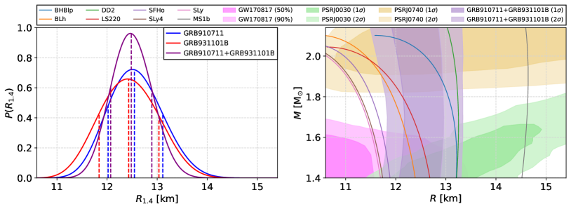
Figure 4: Left: Posterior probability distributions for the radius of a 1.4 M_⊙ NS for GRB 910711, GRB 931101B, and both. The dashed lines represent the median and the $\pm 1\sigma$ values. Right: Credible regions (1$\sigma$ and 2$\sigma$) on the mass-radius plane from joint constraint for both GRBs. We also show the mass-radius curves for the EOSs used in the NR simulations, and the credible regions for the joint mass-radius measurements obtained from GW observations for GW170817 (Abbott et al., 2018a) and X-ray observations for PSR J0030+0451 (e.g., Miller et al. 2019) and PSR J0740+6620 (e.g., Miller et al. 2021).

Table 4: Inferred radii of NSs with mass in the range [1.4, 2.14] M_⊙ (restricted from the validity of the quasiuniversal relations in Godzieba & Radice 2021), that we determined with the binary tidal deformability $\tilde{\Lambda}$ and the chirp mass $\mathcal{M}$ for each GRB and both. The value for $R_{1.4}$ is consistent with current bounds, e.g., $R_{1.4}=12.57^{+0.49}_{-0.48}$ km (Dittmann et al., 2024).

GRB	$R_{1.4}$ [km]	$R_{1.5}$ [km]	$R_{1.6}$ [km]	$R_{1.7}$ [km]	$R_{1.8}$ [km]	$R_{1.9}$ [km]	$R_{2.0}$ [km]	$R_{2.14}$ [km]
910711	$12.55^{+0.56}_{-0.53}$	$12.59^{+0.55}_{-0.52}$	$12.61^{+0.54}_{-0.51}$	$12.61^{+0.54}_{-0.51}$	$12.59^{+0.55}_{-0.51}$	$12.55^{+0.58}_{-0.56}$	$12.52^{+0.61}_{-0.60}$	$12.44^{+0.65}_{-0.63}$
931101B	$12.43^{+0.60}_{-0.59}$	$12.47^{+0.58}_{-0.56}$	$12.51^{+0.56}_{-0.56}$	$12.52^{+0.57}_{-0.56}$	$12.51^{+0.57}_{-0.56}$	$12.48^{+0.60}_{-0.60}$	$12.44^{+0.62}_{-0.62}$	$12.36^{+0.66}_{-0.65}$
910711+931101B	$12.48^{+0.41}_{-0.41}$	$12.52^{+0.41}_{-0.39}$	$12.55^{+0.40}_{-0.39}$	$12.56^{+0.40}_{-0.38}$	$12.54^{+0.40}_{-0.39}$	$12.50^{+0.43}_{-0.40}$	$12.47^{+0.45}_{-0.44}$	$12.39^{+0.47}_{-0.47}$

3 Discussion

We associate the frequencies of the QPOs in GRBs 910711 and 931101B reported by Chirenti et al. (2023) with BNS postmerger oscillation modes and obtain constraints on the redshift of these GRBs, as well as on the chirp mass and binary tidal deformability of the BNS systems whose mergers were presumably their source. We use the redshift to estimate the intrinsic oscillation frequencies of the fundamental quadrupolar mode and the radial mode of the merger remnant in each case, and the chirp mass and tidal deformability to estimate the radius of a 1.4 M_⊙ NS and constrain the mass-radius relation. Therefore, our study introduces a novel way to constrain the EOS of NS matter, using QPOs from short GRBs. Using only two detections, we are able to estimate the radius of a $1.4$ M_⊙ neutron star as $R_{1.4}=12.48^{+0.41}_{-0.41}$ km.

It is important to acknowledge as a caveat that the correspondence between frequencies of QPOs in short GRBs and those in the GW spectrum of BNS mergers is not fully certain. For instance, Most & Quataert (2023) show that strongly magnetized HMNSs can launch mildly relativistic outflows with kilohertz quasiperiodic features, although these features are not necessarily correlated with the postmerger GW signal. In a subsequent study, however, Most et al. (2024) show that the collapse of a rotating magnetar launches an outflow that is modulated by the ringdown of the black hole. Additional modelling and simulations are needed to clarify this scenario.

Future detections of GWs with ground-based detectors such as LIGO, Virgo, and KAGRA, in coincidence with GRBs with QPOs, will allow a test of our model because the GW event will provide independent measurements of the redshift, chirp mass and binary tidal deformability, even if the postmerger signal is not detectable. In the longer term, similar detections with next-generation ground-based detectors will allow for a direct comparison between the postmerger and QPO frequencies.

Finally, we note that the QPOs in Chirenti et al. (2023) also have widths, which can be associated with the damping time of the quadrupolar and radial modes. While the quadrupolar mode is also damped due to the emission of GWs, the radial mode is solely damped through viscosity processes, which play an important role in the stability of remnant (Alford et al., 2018). Therefore, using the QPO widths as a proxy for, or at least a constraint on the damping times of these modes could probe models for the effective viscosity in the remnant.

References

- Abbott et al. (2017a) Abbott, B. P., Abbott, R., Abbott, T. D., et al. 2017a, Phys. Rev. Lett., 119, 161101
- Abbott et al. (2017b) —. 2017b, ApJ, 848, L13
- Abbott et al. (2018a) —. 2018a, Phys. Rev. Lett., 121, 161101
- Abbott et al. (2018b) —. 2018b, Living Reviews in Relativity, 21, 3
- Abbott et al. (2019) —. 2019, Physical Review X, 9, 011001
- Alford et al. (2018) Alford, M. G., Bovard, L., Hanauske, M., Rezzolla, L., & Schwenzer, K. 2018, Phys. Rev. Lett., 120, 041101
- Banik et al. (2014) Banik, S., Hempel, M., & Bandyopadhyay, D. 2014, ApJS, 214, 22
- Baumgarte et al. (2000) Baumgarte, T. W., Shapiro, S. L., & Shibata, M. 2000, ApJ, 528, L29
- Bauswein & Janka (2012) Bauswein, A., & Janka, H. T. 2012, Phys. Rev. Lett., 108, 011101
- Berger (2014) Berger, E. 2014, ARA&A, 52, 43
- Bernuzzi et al. (2016) Bernuzzi, S., Radice, D., Ott, C. D., et al. 2016, Phys. Rev. D, 94, 024023
- Bombaci & Logoteta (2018) Bombaci, I., & Logoteta, D. 2018, A&A, 609, A128
- Breschi et al. (2019) Breschi, M., Bernuzzi, S., Zappa, F., et al. 2019, Phys. Rev. D, 100, 104029
- Chatziioannou et al. (2024) Chatziioannou, K., Cromartie, H. T., Gandolfi, S., et al. 2024, arXiv e-prints, arXiv:2407.11153
- Chirenti et al. (2023) Chirenti, C., Dichiara, S., Lien, A., Miller, M. C., & Preece, R. 2023, Nature, 613, 253
- Chirenti et al. (2019) Chirenti, C., Miller, M. C., Strohmayer, T., & Camp, J. 2019, ApJ, 884, L16
- Choudhury et al. (2024) Choudhury, D., Salmi, T., Vinciguerra, S., et al. 2024, ApJ, 971, L20
- Ciolfi (2018) Ciolfi, R. 2018, International Journal of Modern Physics D, 27, 1842004
- Curtis et al. (2024) Curtis, S., Bosch, P., Mösta, P., et al. 2024, ApJ, 961, L26
- D’Avanzo (2015) D’Avanzo, P. 2015, Journal of High Energy Astrophysics, 7, 73
- De et al. (2018) De, S., Finstad, D., Lattimer, J. M., et al. 2018, Phys. Rev. Lett., 121, 091102
- Dittmann et al. (2024) Dittmann, A. J., Miller, M. C., Lamb, F. K., et al. 2024, arXiv e-prints, arXiv:2406.14467
- Douchin & Haensel (2001) Douchin, F., & Haensel, P. 2001, A&A, 380, 151
- Godzieba & Radice (2021) Godzieba, D. A., & Radice, D. 2021, Universe, 7, 368
- Gonzalez et al. (2023) Gonzalez, A., Zappa, F., Breschi, M., et al. 2023, Classical and Quantum Gravity, 40, 085011
- Guetta & Piran (2005) Guetta, D., & Piran, T. 2005, A&A, 435, 421
- Hempel & Schaffner-Bielich (2010) Hempel, M., & Schaffner-Bielich, J. 2010, Nucl. Phys. A, 837, 210
- Lackey & Wade (2015) Lackey, B. D., & Wade, L. 2015, Phys. Rev. D, 91, 043002
- Lattimer & Swesty (1991) Lattimer, J. M., & Swesty, D. F. 1991, Nucl. Phys. A, 535, 331
- Lioutas et al. (2021) Lioutas, G., Bauswein, A., & Stergioulas, N. 2021, Phys. Rev. D, 104, 043011
- Lü et al. (2015) Lü, H.-J., Zhang, B., Lei, W.-H., Li, Y., & Lasky, P. D. 2015, ApJ, 805, 89
- Miller et al. (2020) Miller, M. C., Chirenti, C., & Lamb, F. K. 2020, ApJ, 888, 12
- Miller et al. (2019) Miller, M. C., Lamb, F. K., Dittmann, A. J., et al. 2019, ApJ, 887, L24
- Miller et al. (2021) —. 2021, ApJ, 918, L28
- Most et al. (2024) Most, E. R., Beloborodov, A. M., & Ripperda, B. 2024, arXiv e-prints, arXiv:2404.01456
- Most & Quataert (2023) Most, E. R., & Quataert, E. 2023, ApJ, 947, L15
- Mösta et al. (2020) Mösta, P., Radice, D., Haas, R., Schnetter, E., & Bernuzzi, S. 2020, ApJ, 901, L37
- Murguia-Berthier et al. (2014) Murguia-Berthier, A., Montes, G., Ramirez-Ruiz, E., De Colle, F., & Lee, W. H. 2014, ApJ, 788, L8
- Nakar (2007) Nakar, E. 2007, Phys. Rep., 442, 166
- Prakash et al. (2024) Prakash, A., Gupta, I., Breschi, M., et al. 2024, Phys. Rev. D, 109, 103008
- Punturo et al. (2010) Punturo, M., Abernathy, M., Acernese, F., et al. 2010, Classical and Quantum Gravity, 27, 194002
- Radice et al. (2020) Radice, D., Bernuzzi, S., & Perego, A. 2020, Annual Review of Nuclear and Particle Science, 70, 95
- Read et al. (2009) Read, J. S., Lackey, B. D., Owen, B. J., & Friedman, J. L. 2009, Phys. Rev. D, 79, 124032
- Reitze et al. (2019) Reitze, D., Adhikari, R. X., Ballmer, S., et al. 2019, in Bulletin of the American Astronomical Society, Vol. 51, 35
- Rezzolla & Takami (2016) Rezzolla, L., & Takami, K. 2016, Phys. Rev. D, 93, 124051
- Riley et al. (2019) Riley, T. E., Watts, A. L., Bogdanov, S., et al. 2019, ApJ, 887, L21
- Riley et al. (2021) Riley, T. E., Watts, A. L., Ray, P. S., et al. 2021, ApJ, 918, L27
- Salmi et al. (2024) Salmi, T., Choudhury, D., Kini, Y., et al. 2024, arXiv e-prints, arXiv:2406.14466
- Sarin & Lasky (2021) Sarin, N., & Lasky, P. D. 2021, General Relativity and Gravitation, 53, 59
- Steiner et al. (2013) Steiner, A. W., Hempel, M., & Fischer, T. 2013, ApJ, 774, 17
- Takami et al. (2015) Takami, K., Rezzolla, L., & Baiotti, L. 2015, Phys. Rev. D, 91, 064001
- Typel et al. (2010) Typel, S., Röpke, G., Klähn, T., Blaschke, D., & Wolter, H. H. 2010, Phys. Rev. C, 81, 015803
- Zhao & Lattimer (2018) Zhao, T., & Lattimer, J. M. 2018, Phys. Rev. D, 98, 063020