The evolution of molecular clouds: global radial collapse

Abstract

The star formation efficiency (SFE) measures the proportion of molecular gas converted into stars, while the star formation rate (SFR) indicates the rate at which gas is transformed into stars. Here we propose such a model in the framework of a global radial collapse of molecular clouds, where the collapse velocity depends on the density profile and the initial mass-to-radius ratio of molecular clouds, with the collapse velocity accelerating during the collapse process. This simplified analytical model allows us to estimate a lifetime of giant molecular clouds of approximately $0.44-7.36\times 10^{7}\,\rm{yr}$, and a star formation timescale of approximately $0.5-5.88\times 10^{6}\,\rm{yr}$. Additionally, we can predict an SFE of approximately $1.59\,\%$, and an SFR of roughly $1.85\,\rm{M_{\odot}\,yr^{-1}}$ for the Milky Way in agreement with observations.

1 Introduction

For several decades, the birth of stars within the Milky Way’s molecular clouds (MCs) has remained at the forefront of astrophysical inquiry (e.g., McKee & Ostriker 2007; Vázquez-Semadeni et al. 2019; Lu et al. 2022; Li et al. 2024). Central to this research are the enigmas surrounding the low SFE of approximately $1\%$ and the low SFR of $1-3\,\rm{M_{\odot}\,yr^{-1}}$ in the Milky Way (e.g., Shu et al. 1987; McKee & Ostriker 2007; Chomiuk & Povich 2011; Davies et al. 2011; Kennicutt & Evans 2012; Licquia & Newman 2015; Elia et al. 2022). The pursuit of the corresponding answers has led to the proposition of theoretical frameworks that shed light on the mechanisms dictating the transformation of MCs into stars.

Various theoretical models and simulations have made substantial efforts to explain the low SFE and SFR (e.g., Krumholz & McKee 2005; Padoan & Nordlund 2011; Vázquez-Semadeni et al. 2019; Padoan et al. 2020). For instance, the global hierarchical collapse model emphasizes that gravity dominates the evolution and dynamics of MCs (Zamora-Avilés & Vázquez-Semadeni 2014; Vázquez-Semadeni et al. 2019). This model suggests that the SFR increases over time, leading star-forming clouds to evolve towards higher SFRs and produce stars with greater average masses. Eventually, feedback from the massive stars begins to disrupt the clouds. Regions that are far enough away, where the infall-motion front has not yet arrived, become decoupled from the collapse due to this feedback. Consequently, this material does not contribute to the star formation episode in the region, keeping the overall SFR low, as observed. In contrast, the initial inflow model highlights the role of supersonic turbulence in massive star formation (Padoan et al. 2020), considering the turbulence as the major factor for both low observed SFE and SFR. However, neither model offers a simple, analytical solution to the low SFE and SFR observed in the Milky Way. Furthermore, gravoturbulent models can explain the low SFR, but involve numerous parameters (Krumholz & McKee 2005), making a direct comparison with observed SFE and SFR not always easy.

In this context, we present a new, streamlined semi-analytical model, termed the global radial collapse (GRC) model. It hypothesizes that an MC, characterized by spherical symmetry in its density distribution, is subject to a global collapse within an isothermal and supersonically turbulent environment. Additionally, the model assumes: (1) the MC exists in (near)isolation and unaffected by magnetic fields, (2) it retains a quasi-static state, upholding a virial equilibrium, and (3) the supersonic turbulence is homogeneous and isotropic. Note that real MCs are not isolated, and their turbulence at small scales (e.g., $\sim 0.01$ pc) deviates from isotropy. Nevertheless, these intricacies are overlooked to maintain the model’s simplicity. Within this model framework, a spherical MC is envisaged to undergo a global, quasi-static collapse radially, driven by its own gravity and regulated by non-negligible turbulence. That is, the supersonic turbulence introduces random local motions that hinder but not halt the MC’s global radial collapse. The initial velocity at the onset of collapse strongly depends on the MC’s density distribution, and its initial mass $M_{0}$ and radius $R_{0}$.

2 The global radial collapse

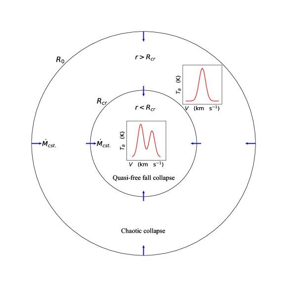
Figure 1: An illustration of the gas radial collapse. The $R_{0}$ represents the boundary of MC, $R_{cr}$ represents the critical transition scale, and $\dot{M}_{cst.}$ represents the constant mass infall rate. In regions where $r>R_{cr}$, the gas undergoing chaotic collapse and the Gaussian spectral lines are readily observed. In regions where $r<R_{cr}$, the gas undergoing quasi-free fall collapse and the blue asymmetric spectral lines are easily observed.

2.1 Constantly mass infall rate $\dot{M}_{cst.}$

We consider MCs as supersonically turbulent gas flows, governed by the mass continuity equation:

$$\frac{\partial\rho}{\partial t}+\nabla\cdot(\rho\vec{u})=0.$$ (1)

The quasi-static approximation of MCs implies $\partial\rho/\partial t=0$, leading to $\nabla\cdot(\rho\vec{u})=0$ with $\vec{u}=(u_{r},u_{\theta},u_{\varphi})$ in a spherical coordinate system. Assuming a spherically symmetric density distribution allows us to consider collapse occurring only in the radial direction, yielding $\vec{u}=u_{r}$. Therefore,

$$\nabla\cdot(\rho\vec{u})=\nabla\cdot(\rho u_{r})=\frac{1}{r^{2}}\frac{\partial}{\partial r}(r^{2}\rho u_{r})=0.$$ (2)

This equation results in a constant mass infall rate

$$\dot{M}_{cst.}=r^{2}\rho u_{r}.$$ (3)

Consequently, the mass of gas passing through any hierarchical, spherical surface remains constant per unit time, as illustrated in Fig. 1.

If the density distribution of spherically symmetric MCs follows a profile of $\rho=\rho_{re}(r/r_{re})^{-p}$ with $\rho_{re}$ known at the reference $r_{re}$, we can derive:

$$\dot{M}_{cst.}=r_{re}^{2}\rho_{re}u_{r}\left(\frac{r}{r_{re}}\right)^{2-p}.$$ (4)

Furthermore, the collapse velocity $u_{r}$ can be expressed as:

$$u_{r}=\frac{\dot{M}_{cst.}}{\rho_{re}r_{re}^{2}}\left(\frac{r}{r_{re}}\right)^{p-2}.$$ (5)

For $p=2$, a constant velocity emerges, indicating a scale-free gravitational collapse (Li 2018), akin to the collapse of the envelope of a hydrostatic singular isothermal sphere (Shu 1977). However, when $p<2$, $u_{r}$ increases as $r$ decreases, suggesting that the collapse velocity accelerates down to smaller scales where star formation occurs. This increasing trend of collapse velocity with decreasing scale has been supported by observations toward high-mass star formation regions (Yang et al. 2023).

2.2 Critical transition scale $R_{cr}$

The density distribution $\rho=\rho_{re}(r/r_{re})^{-p}$ yields the gravitational potential energy $U$ as follows (Bertoldi & McKee 1992):

$$U=-\frac{3-p}{5-2p}\frac{GM^{2}}{r}.$$ (6)

The kinetic energy $E_{k}$ includes contributions from supersonic turbulence ($E_{turb}$), thermal motions ($E_{ther}$), and the kinetic motions of infall gas resulting from self-gravitational collapse ($E_{a}$). Since both thermal and turbulent motions counteract the self-gravity of MCs, and with supersonic turbulent motions significantly stronger than thermal motions ($E_{turb}\gg E_{ther}$), we combine them as $E_{t}=E_{turb}+E_{ther}\approx E_{turb}$.

For an MC in a state of virial equilibrium, the potential energy is equal to twice the kinetic energy (Bertoldi & McKee 1992),

$$2E_{k}+U=0\Leftrightarrow\mid-U\mid=2(E_{t}+E_{a}).$$ (7)

In the case where all gravitational energy is converted to infall kinetic energy, corresponding to $E_{t}=0$ without any support against gravity, the equation simplifies to $\mid-U\mid=2E_{a}$. Substituting this relation into Eq. 6, we derive the initial collapse velocity $u_{0}$ of the MCs at $R_{0}$ as follows:

$$u_{0}=\frac{2E_{a,0}}{M_{0}}=\left(\frac{3-p}{5-2p}\frac{GM_{0}}{R_{0}}\right)^{1/2}.$$ (8)

According to Eq. 5, when the collapse velocity at any radius has $u_{r}=u_{0}$, indicating unhindered gas collapse at the initial moment, which corresponds to $p=2$ and leads to $\dot{M}_{cst.}=r_{re}^{2}\rho_{re}u_{0}$. Because gas collapse is solely induced by self-gravity, the $\dot{M}_{cst.}$ remains independent of whether the gas is supported or not for a given cloud with an initial mass $M_{0}$ and initial radius $R_{0}$. That is, turbulent support slows down the speed of gas falling but does not reduce the mass of gas falling per unit time. Therefore, Eq. 5 can be re-expressed as:

$$u_{r}=u_{0}\left(\frac{r}{r_{re}}\right)^{p-2}.$$ (9)

From Eq. 9, the collapse velocity $u_{r}$ is small on large scales, making the $E_{t}$ become the primary contributor to the kinetic energy $E_{k}$. Due to the dissipation of turbulence and the acceleration of collapse velocity, $u_{r}$ will exceed the turbulent velocity at a critical transition scale $R_{cr}$, thereby dominating the energy balance. Consequently, we expect $R_{cr}$ to appear at the scale where the turbulent velocity equals $u_{r}$. If turbulent velocity dissipation follows $\sigma=\sigma_{re}(r/r_{re})^{\beta}$, where $\beta=1-p/2$ for an MC maintaining virial equilibrium (McKee & Tan 2003; Luo et al. 2024), the equality of the turbulent and collapse velocities gives rise to:

$$\sigma_{re}\left(\frac{r}{r_{re}}\right)^{1-p/2}=u_{0}\left(\frac{r}{r_{re}}\right)^{p-2}.$$ (10)

Replacing $r$ with $R_{cr}$ in this equation, we obtain:

$$\frac{R_{cr}}{r_{re}}=\left(\frac{\sigma_{re}}{u_{0}}\right)^{2/(3p-6)}.$$ (11)

For $r>R_{cr}$, where $\sigma>u_{r}$, turbulence dominates the velocity field, leading to chaotic collapse behavior. In this region, the gas is not expected to directly participate in the star formation process due to the randomness of the collapse. Consequently, the chaotic collapse velocity will hardly produce the blue asymmetric spectra in line emission of gravitational collapse tracers, making it difficult to observe. For $r<R_{cr}$, where $u_{r}>\sigma$, the collapse velocity dominates over the turbulent velocity. Thus, the collapse within $R_{cr}$ is anticipated to resemble a quasi-free fall collapse. The gas within this region can directly participate in the star formation process. If real clouds possess a homogeneous and spherically symmetric density distribution, the velocity field dominated by ordered collapse motions will result in observable blue asymmetric molecular emission lines (as shown in Fig. 1). Note that Eq. 11 becomes invalid when $p=2$, indicating the absence of a critical transition scale. This may mean that the gas throughout the entire spherical framework can participate in the formation of stars for the scenarios of scale-free gravitational collapse (Li 2018).

2.3 SFE and SFR

Based on the collapse velocity, we can define the gas infall time as:

$$dt=\frac{dr}{u_{r}}\Leftrightarrow dt=\frac{(r/{r_{re}})^{2-p}}{u_{0}}dr.$$ (12)

We define the time when the gas to travel from the boundary $R_{0}$ to the gravitational center of MCs as $t_{MC}$:

$$t_{MC}=\frac{r_{re}}{(3-p)u_{0}}\left(\frac{R_{0}}{r_{re}}\right)^{3-p}.$$ (13)

If the collapse and evolution of an MC are (nearly)isolated, $t_{MC}$ can be taken to approximate the cloud lifetime.

Similarly, we express the time required for the gas from the critical transition scale $R_{cr}$ to the gravitational center of MCs as $t_{cr}$:

$$t_{cr}=\frac{r_{re}}{(3-p)u_{0}}\left(\frac{R_{cr}}{r_{re}}\right)^{3-p}.$$ (14)

Since only the gas within the region of $r<R_{cr}$ can effectively participate in star formation, $t_{cr}$ can serve as a reasonable approximation of the star formation timescale.

Therefore, in a molecular cloud, the total gas mass available for star formation is $M_{cr}=\dot{M}_{cst.}\cdot t_{cr}$. This mass ultimately transfers to the precursors that form stars, i.e. , prestellar cores. However, due to the conversion efficiency of $\epsilon\sim 0.25-0.75$ from prestellar cores to newborn stars (e.g., Matzner & McKee 2000; Tanaka et al. 2017; Staff et al. 2019), the mass $M_{cr}$ relates to the stellar mass via $M_{*}=M_{cr}\cdot\epsilon$. The SFE over the time interval $t_{MC}$ can then be determined as:

$$\mathrm{SFE}=\frac{M_{*}}{M_{0}}.$$ (15)

Given $M_{*}=M_{cr}\cdot\epsilon=\dot{M}_{cst.}\cdot t_{cr}\cdot\epsilon$, Eq. 15 indicates that an extended $t_{cr}$ (depending on the density profile, $\sigma_{re}$, and $u_{0}$) and an increased $\dot{M}_{cst.}$ (depending on the density profile and $u_{0}$) enhance the efficiency with which an MC converts its gas into new stars.

Moreover, the SFR for an MC over their lifetimes can be expressed as:

$$\mathrm{SFR}=\frac{M_{*}}{t_{MC}}=\mathrm{SFE}\cdot\frac{M_{0}}{t_{MC}}.$$ (16)

Recalling $M_{*}=\dot{M}_{cst.}\cdot t_{cr}\cdot\epsilon$, Eq. 16 suggests an increase in $t_{cr}$ or $\dot{M}_{cst.}$ serves to accelerate the star formation process. This depends on the enhanced self-gravity of MCs, leading to a faster collapse and an earlier initiation of gas into star formation. As a result, both a high SFR and SFE are the natural outcomes of the strong self-gravity of MCs, which is further influenced by the clouds’ density structure and the level of turbulence.

Assuming that MCs in the Milky Way have similar SFEs, we can estimate the SFR of the Milky Way over the period $t_{MC}$ as:

$$\mathrm{SFR_{MW}}\simeq\mathrm{SFE}\cdot\frac{M_{\mathrm{{gas}}}}{t_{MC}},$$ (17)

where $M_{\mathrm{{gas}}}$ is the total mass of MCs in the Milky Way.

3 Comparison with observations

Our model can be used to elucidate various observable parameters. For illustration, we leverage data from 158 giant molecular clouds (GMCs) observed in the Boston University-FCRAO Galactic Ring Survey (GRS) (e.g., Heyer et al. 2009). The dataset reflects a global virial equilibrium state for GMCs and unveils a density profile for them of $\rho=\rho_{re}(r/r_{re})^{-1.54}$, alongside a velocity dispersion profile of $\sigma=\sigma_{re}(r/r_{re})^{0.26}$, where $\rho_{re}$ is $2.2\times 10^{-20}$  g $\mbox{~{}cm}^{-3}$, $\sigma_{re}$ is $1.16$ km s^-1, and $r_{re}$ is 1  pc (Luo et al. 2024). By integrating these empirical relationships into our framework, we have computed several key parameters for the GMCs, which are compiled in Appendix Table 2 and summarised in Table 1.

Table 1: Summary of the main parameters for 158 GMCs.

Parameter	Unit	Mean	Median	Max	Min
$\dot{M}_{cst.}$	$10^{-3}\rm{\,M_{\odot}\,yr^{-1}}$	1.04	1.0	3.08	0.33
$R_{cr}$	pc	4.52	3.86	20.35	0.81
$t_{MC}$	$10^{7}\,\rm{yr}$	1.71	1.73	7.36	0.44
$t_{cr}$	$10^{6}\,\rm{yr}$	1.56	1.63	5.88	0.50
$M_{*}$	$\rm{M_{\odot}}$	1166	800	9061	82
SFE	$\%$	1.86	1.59	6.01	0.36
SFR	$\rm{10^{-5}\,M_{\odot}\,yr^{-1}}$	6.96	4.28	67.62	0.42

The transition of MCs from a state of chaotic collapse to a quasi-free fall collapse occurs at a critical radius, $R_{cr}$. Analysis of 158 GMCs reveals that $R_{cr}$ has a median of $3.86$ pc and an average of $4.52$ pc, covering a range between 1 pc and 6 pc (refer to Appendix Fig. 3 b) which correspond to the clump scales (e.g., Heyer & Dame 2015; Ballesteros-Paredes et al. 2020; Peretto et al. 2023). The time $t_{MC}$, varies from $0.44-7.36\times 10^{7}\,\rm{yr}$, and the critical time, $t_{cr}$, spans $0.5-5.88\times 10^{6}\,\rm{yr}$, both displaying similar distributions. Note that the average and median $t_{MC}$ are $1.71\times 10^{7}\,\rm{yr}$ and $1.73\times 10^{7}\,\rm{yr}$, respectively, while for $t_{cr}$, they are $1.56\times 10^{6}\,\rm{yr}$ and $1.63\times 10^{6}\,\rm{yr}$, respectively. Therefore, we anticipate that the lifetime of GMCs could be approximately $10^{7}\,\rm{yr}$, as confirmed by previous studies (e.g., Chevance et al. 2020; Jeffreson et al. 2021; Chevance et al. 2023). We also expect the star formation timescale to be around $10^{6}\,\rm{yr}$, which aligns with simulation results (e.g., Padoan et al. 2020; Grudić et al. 2022). Nevertheless, further observations are needed to validate these predictions.

Our model assumes a constant mass infall rate (see Eq. 3), which is approximately $10^{-3}$ $\rm{M_{\odot}\,yr^{-1}}$ for the GMCs in our Milky Way (see Table 1). Naturally, GMCs with different initial conditions exhibit varying mass infall rates, with differences reaching an order of magnitude ($\dot{M}_{cst.}\sim 0.33-3.08\times 10^{-3}\,\rm{M_{\odot}\,yr^{-1}}$). Based on Eq. 15 and assuming a typical value of $\epsilon\simeq 0.5$, we estimated the SFEs for 158 GMCs in our Milky Way. The mean and median SFEs are 1.86 % and 1.59 %, respectively, consistent with the low SFE observed for the Milky Way (e.g., McKee & Ostriker 2007; Krumholz & Tan 2007). Furthermore, the SFRs for 158 GMCs vary from $0.42-67.62\times 10^{-5}\,\rm{M_{\odot}\,yr^{-1}}$, which is in agreement with observations (Lada et al. 2010).

Likewise, assuming a uniform spatial distribution of GMCs in the Milky Way, we can estimate the average SFR for the Milky Way using Eq. 17 as follows:

$$\mathrm{SFR_{MW}}\simeq 0.0159\cdot\frac{2\times 10^{9}\,\rm{M_{\odot}}}{1.73\times 10^{7}\,\rm{yr}}=1.85\,\rm{M_{\odot}\,yr^{-1}}.$$ (18)

Here, we utilized the median values of SFE and $t_{MC}$ for the 158 GMCs, along with its total molecular gas mass of $2\times 10^{9}\,\rm{M_{\odot}}$ (e.g., Ferrière 2001; Klessen & Hennebelle 2010). The resulting average SFR agrees with current observational results (e.g., Elia et al. 2022; Chomiuk & Povich 2011; Davies et al. 2011; Licquia & Newman 2015).

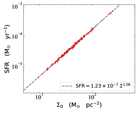
Figure 2: The relation between SFR and gas surface density for the 158 giant molecular cloud.

Moreover, our model allows us to predict the relationship between the SFR and the initial gas surface density for GMCs:

$$\mathrm{SFR}\propto\Sigma_{0}^{\frac{12-5p}{12-6p}}\cdot R_{0}^{\frac{-24+25p-6p^{2}}{12-6p}},$$ (19)

where the initial gas surface density is $\Sigma_{0}=M_{0}/(\pi R_{0}^{2})$. For $p=-1.54$, the power index $\frac{12-5p}{12-6p}\simeq 1.56$. However, when $p=1.5$, $\frac{-24+25p-6p^{2}}{12-6p}=0$, indicating that the SFR depends solely on $\Sigma_{0}$. Given a conversion efficiency $\epsilon=0.5$, the relationship between SFR and $\Sigma_{0}$ for the GMC sample from the GRS survey is (see Fig. 2):

$$\mathrm{SFR}\simeq 1.23\times 10^{-7}\cdot\left(\frac{\Sigma_{0}}{\mathrm{M_{\odot}\cdot pc^{-2}}}\right)^{1.58}\,\rm{M_{\odot}\cdot yr^{-1}}.$$ (20)

This predicted SFR–$\Sigma_{0}$ relationship highlights that denser initial conditions of MCs lead to higher SFRs, warranting further validation by future observations. It is worth noting that a power-law relationship between the SFR per unit area of galaxies and their gas surface density, i.e. , the Kennicutt-Schmidt (K-S) law (Kennicutt 1998), has been widely discussed. However, our GRC model cannot reproduce the empirical K-S relation, which will be addressed in future work.

It should be noted that further observations are needed to validate the density profile and velocity dispersion scaling relation we used. The observed velocity dispersion scaling relation is generally of the form $\sigma\propto r^{\beta}$, with a power-law exponent $\beta\sim 0.5$, which is higher than 0.26 adopted in this work. The latter value was interpreted as a possible result of added contribution of magnetic fields to turbulence. However, different velocity dispersion scaling relations may correspond to different density distributions (e.g., Larson 1981; McKee & Tan 2003; Luo et al. 2024). Therefore, we expect that if MCs are in virial equilibrium, applying different density distributions and velocity dispersion scaling relations to the GRC model can still yield similar results.

4 summary

Our new semi-analytical model describes the global radial collapse of an MC. It emphasizes that the MC is always undergoing global collapse in the radial direction, while highlighting the different collapse regions and that the variations in collapse modes regulated by turbulence. The GRC model has successfully reproduced the low SFE and SFR observed within the Milky Way. Additionally, this model facilitates the prediction of various observational indices, including the lifespan of GMCs, star formation time, and both the SFE and SFR for individual MCs. Future validation of this model with new observational data will refine the radial collapse paradigm, providing promising insights into the evolution of molecular clouds into stars.

We carried out this work at the China-Argentina Cooperation Station of NAOC/CAS. This work was supported by the Key Project of Inter national Cooperation of Ministry of Science and Technology of China through grant 2010DFA02710, and by the National Key R&D Program of China (No. 2022YFA1603101). H.-L. Liu is supported by National Natural Science Foundation of China (NSFC) through the grant No. 12103045, by Yunnan Fundamental Research Project (grant No. 202301AT070118, 202401AS070121), and by Xingdian Talent Support Plan–Youth Project.

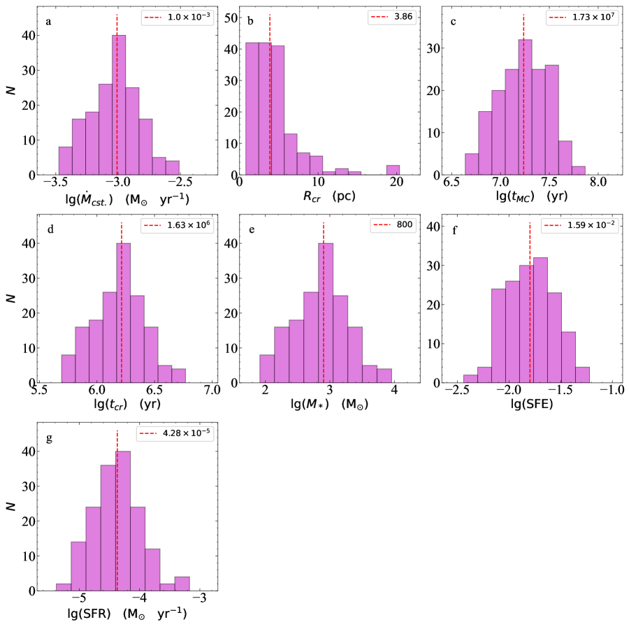
Figure 3: The histogram distribution of seven important parameters.

Table 2: The physical parameters of 158 GMCs

GMC	$R_{0}$	$M_{0}$	$u_{0}$	$\dot{M_{0}}$	$R_{cr}$	$t_{MC}$	$t_{cr}$	$M_{*}$	SFE	SFR
	pc	$\rm{M_{\odot}}$	km s-1	$\rm{M_{\odot}\,yr^{-1}}$	pc	yr	yr	$\rm{M_{\odot}}$		$\rm{M_{\odot}\,yr^{-1}}$
		$10^{4}$		$10^{-3}$		$10^{7}$	$10^{6}$		$10^{-2}$	$10^{-5}$
GMC 64	40.6	32.0	5.08	1.69	8.5	2.94	3.0	2531	0.79	8.6
GMC 67	42.2	7.9	2.47	0.82	3.0	6.39	1.34	553	0.7	0.87
GMC 68	6.9	1.4	2.58	0.86	3.18	0.44	1.41	602	4.3	13.81
GMC 70	9.7	1.3	2.09	0.7	2.35	0.88	1.12	388	2.99	4.4
GMC 71	10.3	1.9	2.46	0.82	2.97	0.82	1.33	544	2.87	6.63
GMC 72	41.3	26.0	4.54	1.51	7.22	3.38	2.65	1995	0.77	5.91
GMC 73	4.6	0.28	1.41	0.47	1.33	0.44	0.72	168	6.02	3.82
GMC 74	32.1	11.0	3.35	1.11	4.65	3.17	1.88	1048	0.95	3.31
GMC 75	23.2	13.0	4.28	1.42	6.64	1.54	2.48	1764	1.36	11.44
GMC 77	33.8	12.0	3.41	1.13	4.77	3.35	1.92	1088	0.91	3.24
GMC 78	22.8	7.8	3.34	1.11	4.64	1.92	1.88	1047	1.34	5.44
GMC 79	27.1	19.0	4.79	1.59	7.81	1.73	2.81	2236	1.18	12.93
GMC 80	16.7	2.0	1.98	0.66	2.17	2.06	1.05	345	1.72	1.67
GMC 81	45.0	23.0	4.09	1.36	6.21	4.25	2.35	1600	0.7	3.77
GMC 82	15.3	1.0	1.46	0.49	1.4	2.46	0.75	182	1.82	0.74
GMC 84	23.7	4.9	2.6	0.86	3.22	2.62	1.42	614	1.25	2.35
GMC 85	18.1	2.4	2.08	0.69	2.33	2.21	1.11	384	1.6	1.74
GMC 86	32.0	12.0	3.5	1.16	4.96	3.01	1.98	1153	0.96	3.83
GMC 87	7.5	0.35	1.24	0.41	1.1	1.03	0.62	127	3.63	1.24
GMC 88	46.0	20.0	3.77	1.25	5.52	4.75	2.15	1349	0.67	2.84
GMC 89	22.9	6.2	2.98	0.99	3.92	2.18	1.65	817	1.32	3.75
GMC 90	18.4	5.8	3.21	1.07	4.37	1.47	1.8	960	1.65	6.55
GMC 91	17.1	4.4	2.9	0.96	3.78	1.46	1.61	774	1.76	5.31
GMC 92	10.6	0.34	1.02	0.34	0.83	2.05	0.5	86	2.52	0.42
GMC 93	11.4	9.2	5.14	1.71	8.64	0.46	3.04	2595	2.82	57.0
GMC 94	16.0	5.6	3.38	1.12	4.72	1.13	1.91	1072	1.91	9.46
GMC 95	19.8	4.0	2.57	0.85	3.17	2.04	1.4	599	1.5	2.94
GMC 96	6.4	0.53	1.65	0.55	1.66	0.61	0.85	233	4.4	3.81
GMC 97	83.4	210.0	9.07	3.02	19.71	4.71	5.73	8648	0.41	18.36
GMC 98	28.2	12.0	3.73	1.24	5.44	2.35	2.13	1318	1.1	5.6
GMC 99	8.8	0.67	1.58	0.52	1.56	1.02	0.81	213	3.19	2.1
GMC 100	23.3	41.0	7.59	2.52	15.2	0.88	4.69	5919	1.44	67.62
GMC 101	11.6	1.4	1.99	0.66	2.18	1.21	1.05	348	2.48	2.88
GMC 102	29.8	42.0	6.79	2.26	12.95	1.4	4.15	4680	1.11	33.41
GMC 103	9.7	0.58	1.4	0.46	1.31	1.32	0.71	165	2.85	1.25
GMC 105	8.2	2.1	2.89	0.96	3.76	0.5	1.6	770	3.67	15.42
GMC 106	22.7	8.2	3.44	1.14	4.83	1.86	1.94	1109	1.35	5.96
GMC 107	5.7	0.46	1.62	0.54	1.63	0.52	0.84	227	4.94	4.34
GMC 109	25.4	5.3	2.61	0.87	3.24	2.88	1.43	620	1.17	2.15
GMC 110	19.3	12.0	4.51	1.5	7.15	1.12	2.63	1969	1.64	17.6
GMC 111	9.7	2.5	2.9	0.97	3.78	0.64	1.61	776	3.1	12.19
GMC 112	20.2	3.8	2.48	0.82	3.01	2.17	1.35	556	1.46	2.56
GMC 113	9.1	0.77	1.66	0.55	1.69	1.01	0.86	239	3.1	2.36
GMC 114	26.4	12.0	3.86	1.28	5.7	2.07	2.21	1414	1.18	6.84
GMC 115	12.0	4.2	3.38	1.12	4.72	0.75	1.91	1072	2.55	14.39
GMC 116	25.8	6.9	2.96	0.98	3.88	2.61	1.64	807	1.17	3.1
GMC 117	26.3	11.0	3.7	1.23	5.37	2.14	2.11	1295	1.18	6.04
GMC 118	23.3	12.0	4.1	1.36	6.24	1.62	2.36	1613	1.34	9.97
GMC 119	34.7	9.1	2.93	0.97	3.83	4.06	1.62	790	0.87	1.95
GMC 120	7.3	0.44	1.4	0.47	1.32	0.87	0.71	167	3.79	1.92
GMC 121	52.0	59.0	6.09	2.03	11.06	3.52	3.67	3721	0.63	10.57
GMC 122	53.7	55.0	5.79	1.92	10.27	3.88	3.47	3339	0.61	8.6
GMC 123	16.3	1.9	1.95	0.65	2.13	2.02	1.03	335	1.76	1.66
GMC 124	17.9	3.2	2.42	0.8	2.9	1.87	1.31	527	1.65	2.82
GMC 125	42.7	15.0	3.39	1.13	4.73	4.74	1.91	1076	0.72	2.27
GMC 126	7.2	0.36	1.28	0.43	1.15	0.93	0.64	137	3.8	1.46
GMC 127	34.0	12.0	3.4	1.13	4.75	3.39	1.92	1082	0.9	3.19
GMC 128	37.4	21.0	4.29	1.42	6.65	3.09	2.48	1768	0.84	5.72
GMC 129	9.6	0.41	1.18	0.39	1.03	1.54	0.59	116	2.82	0.75
GMC 130	12.8	1.0	1.6	0.53	1.59	1.73	0.83	219	2.19	1.27
GMC 131	8.4	0.7	1.65	0.55	1.67	0.91	0.86	235	3.36	2.59
GMC 133	16.1	4.5	3.02	1.01	4.01	1.28	1.68	845	1.88	6.6
GMC 134	25.8	15.0	4.36	1.45	6.81	1.77	2.53	1834	1.22	10.38
GMC 135	38.5	8.1	2.62	0.87	3.26	5.27	1.44	626	0.77	1.19
GMC 136	12.2	0.79	1.46	0.48	1.39	1.77	0.74	180	2.28	1.01
GMC 137	12.5	0.7	1.35	0.45	1.25	1.98	0.69	154	2.2	0.78
GMC 138	16.9	3.0	2.41	0.8	2.88	1.72	1.31	523	1.74	3.03
GMC 139	6.1	0.26	1.18	0.39	1.03	0.79	0.59	116	4.44	1.45
GMC 140	17.7	1.4	1.61	0.53	1.61	2.76	0.83	222	1.59	0.8
GMC 141	14.8	1.8	1.99	0.66	2.19	1.72	1.06	350	1.95	2.04
GMC 142	29.0	13.0	3.83	1.27	5.64	2.39	2.19	1393	1.07	5.84
GMC 143	10.5	0.64	1.41	0.47	1.33	1.47	0.72	169	2.64	1.15
GMC 144	9.2	1.7	2.46	0.82	2.97	0.7	1.33	545	3.21	7.84
GMC 145	17.0	1.9	1.91	0.64	2.06	2.19	1.01	320	1.69	1.46
GMC 146	23.3	16.0	4.74	1.58	7.69	1.4	2.78	2187	1.37	15.61
GMC 147	15.0	2.2	2.19	0.73	2.51	1.59	1.17	427	1.94	2.68
GMC 148	37.2	25.0	4.69	1.56	7.57	2.8	2.74	2138	0.86	7.62
GMC 149	19.5	8.3	3.73	1.24	5.44	1.37	2.13	1319	1.59	9.61
GMC 150	13.8	2.6	2.48	0.83	3.01	1.25	1.35	557	2.14	4.47
GMC 151	24.3	22.0	5.44	1.81	9.39	1.3	3.24	2930	1.33	22.58
GMC 152	26.5	22.0	5.21	1.73	8.82	1.54	3.09	2674	1.22	17.38
GMC 153	16.6	6.7	3.63	1.21	5.23	1.11	2.06	1247	1.86	11.19
GMC 154	16.3	3.2	2.53	0.84	3.1	1.56	1.38	582	1.82	3.74
GMC 155	31.6	18.0	4.32	1.43	6.71	2.4	2.5	1795	1.0	7.48
GMC 156	9.4	0.94	1.81	0.6	1.9	0.98	0.95	285	3.03	2.92
GMC 157	23.8	9.7	3.65	1.21	5.27	1.88	2.08	1260	1.3	6.71
GMC 158	41.1	37.0	5.43	1.8	9.36	2.8	3.23	2913	0.79	10.39
GMC 159	14.0	2.8	2.56	0.85	3.15	1.23	1.4	593	2.12	4.81
GMC 160	19.9	5.9	3.11	1.04	4.18	1.69	1.74	900	1.52	5.31
GMC 161	40.8	27.0	4.65	1.55	7.49	3.23	2.72	2103	0.78	6.5
GMC 162	34.9	83.0	8.82	2.93	18.91	1.36	5.55	8141	0.98	59.94
GMC 163	12.9	3.4	2.94	0.98	3.84	0.95	1.63	794	2.34	8.32
GMC 164	13.2	2.0	2.23	0.74	2.57	1.3	1.19	442	2.21	3.4
GMC 165	5.0	0.17	1.05	0.35	0.87	0.67	0.52	91	5.35	1.37
GMC 167	26.1	8.7	3.3	1.1	4.55	2.37	1.86	1018	1.17	4.29
GMC 168	44.7	27.0	4.44	1.48	7.01	3.87	2.58	1910	0.71	4.94
GMC 169	14.4	3.4	2.78	0.92	3.55	1.18	1.53	707	2.08	5.97
GMC 170	19.4	3.2	2.32	0.77	2.74	2.19	1.25	484	1.51	2.21
GMC 171	41.8	110.0	9.28	3.08	20.35	1.68	5.88	9061	0.82	53.93
GMC 172	8.8	0.69	1.6	0.53	1.6	1.0	0.83	220	3.19	2.2
GMC 173	8.4	0.26	1.01	0.33	0.81	1.49	0.49	82	3.17	0.55
GMC 174	36.2	22.0	4.46	1.48	7.04	2.83	2.59	1922	0.87	6.78
GMC 175	12.5	4.0	3.24	1.08	4.42	0.83	1.81	975	2.44	11.79
GMC 177	14.7	4.8	3.27	1.09	4.49	1.04	1.83	996	2.08	9.6
GMC 178	58.6	51.0	5.34	1.77	9.13	4.78	3.17	2811	0.55	5.87
GMC 179	13.6	1.6	1.96	0.65	2.14	1.54	1.04	338	2.11	2.19
GMC 180	21.9	8.9	3.65	1.21	5.26	1.66	2.07	1256	1.41	7.55
GMC 181	19.0	3.1	2.31	0.77	2.71	2.13	1.25	478	1.54	2.24
GMC 182	37.7	16.0	3.73	1.24	5.43	3.6	2.12	1315	0.82	3.65
GMC 183	15.0	4.0	2.95	0.98	3.87	1.18	1.64	804	2.01	6.8
GMC 184	44.4	14.0	3.21	1.07	4.37	5.3	1.8	960	0.69	1.81
GMC 185	23.0	2.8	2.0	0.66	2.19	3.27	1.06	351	1.25	1.07
GMC 186	34.0	11.0	3.25	1.08	4.46	3.54	1.82	987	0.9	2.78
GMC 187	35.7	11.0	3.17	1.06	4.3	3.9	1.78	937	0.85	2.4
GMC 188	32.9	12.0	3.45	1.15	4.86	3.18	1.95	1120	0.93	3.52
GMC 189	21.3	3.1	2.18	0.73	2.5	2.67	1.17	424	1.37	1.59
GMC 190	19.9	2.5	2.03	0.67	2.25	2.6	1.08	363	1.45	1.39
GMC 191	30.1	7.8	2.91	0.97	3.79	3.32	1.61	780	1.0	2.35
GMC 192	21.5	3.6	2.34	0.78	2.77	2.52	1.26	491	1.37	1.95
GMC 193	18.1	11.0	4.46	1.48	7.04	1.03	2.59	1922	1.75	18.66
GMC 195	7.6	0.79	1.84	0.61	1.96	0.7	0.97	297	3.76	4.23
GMC 196	16.1	3.4	2.63	0.87	3.27	1.47	1.44	628	1.85	4.26
GMC 198	15.7	3.6	2.74	0.91	3.47	1.36	1.51	685	1.9	5.03
GMC 202	36.0	14.0	3.57	1.19	5.09	3.51	2.02	1199	0.86	3.41
GMC 203	12.8	0.78	1.41	0.47	1.33	1.96	0.72	169	2.16	0.86
GMC 204	6.4	0.45	1.52	0.5	1.47	0.66	0.78	196	4.36	2.96
GMC 205	31.7	7.4	2.76	0.92	3.52	3.77	1.52	698	0.94	1.85
GMC 206	17.2	5.1	3.11	1.04	4.18	1.37	1.74	900	1.76	6.57
GMC 207	25.3	6.0	2.78	0.93	3.56	2.69	1.53	710	1.18	2.64
GMC 208	13.9	3.7	2.95	0.98	3.87	1.06	1.64	803	2.17	7.58
GMC 209	31.8	12.0	3.51	1.17	4.98	2.98	1.99	1161	0.97	3.9
GMC 210	6.4	0.3	1.24	0.41	1.1	0.81	0.62	128	4.26	1.57
GMC 211	20.8	7.7	3.48	1.16	4.91	1.62	1.97	1138	1.48	7.04
GMC 212	10.8	3.2	3.11	1.03	4.18	0.69	1.74	899	2.81	12.95
GMC 213	10.8	2.3	2.64	0.88	3.29	0.82	1.44	634	2.76	7.74
GMC 214	90.8	120.0	6.57	2.19	12.36	7.36	4.0	4372	0.36	5.94
GMC 215	12.5	0.84	1.48	0.49	1.43	1.8	0.76	187	2.23	1.04
GMC 216	11.4	1.3	1.93	0.64	2.09	1.21	1.02	327	2.52	2.7
GMC 217	42.6	25.0	4.38	1.46	6.86	3.66	2.54	1852	0.74	5.06
GMC 218	25.3	6.7	2.94	0.98	3.85	2.54	1.63	798	1.19	3.14
GMC 219	20.6	6.3	3.16	1.05	4.28	1.75	1.77	930	1.48	5.3
GMC 220	15.9	5.5	3.36	1.12	4.68	1.13	1.89	1059	1.93	9.37
GMC 221	16.9	5.7	3.32	1.1	4.59	1.25	1.87	1031	1.81	8.24
GMC 223	7.1	0.68	1.77	0.59	1.84	0.66	0.93	272	4.0	4.11
GMC 224	46.1	46.0	5.71	1.9	10.08	3.15	3.42	3248	0.71	10.32
GMC 225	47.0	44.0	5.53	1.84	9.62	3.34	3.3	3036	0.69	9.08
GMC 226	13.6	5.8	3.73	1.24	5.44	0.81	2.13	1321	2.28	16.31
GMC 227	19.8	6.8	3.35	1.11	4.65	1.56	1.89	1051	1.55	6.73
GMC 229	17.7	2.0	1.92	0.64	2.08	2.31	1.01	324	1.62	1.4
GMC 232	32.0	13.0	3.65	1.21	5.26	2.9	2.07	1255	0.97	4.34
GMC 234	11.9	1.9	2.29	0.76	2.67	1.09	1.23	467	2.46	4.29
GMC 236	7.3	0.77	1.86	0.62	1.98	0.66	0.98	301	3.91	4.59
GMC 237	31.3	10.0	3.23	1.07	4.42	3.16	1.81	974	0.97	3.08
GMC 238	12.3	1.9	2.25	0.75	2.61	1.16	1.21	451	2.38	3.88
GMC 240	9.0	1.3	2.17	0.72	2.48	0.76	1.16	420	3.23	5.52
GMC 241	15.9	2.3	2.18	0.72	2.49	1.75	1.16	421	1.83	2.41
GMC 242	12.8	5.0	3.57	1.19	5.11	0.77	2.03	1204	2.41	15.54
GMC 243	28.2	11.0	3.57	1.19	5.1	2.46	2.03	1202	1.09	4.89

References

- Ballesteros-Paredes et al. (2020) Ballesteros-Paredes, J., André, P., Hennebelle, P., et al. 2020, Space Sci. Rev., 216, 76, doi: 10.1007/s11214-020-00698-3
- Bertoldi & McKee (1992) Bertoldi, F., & McKee, C. F. 1992, ApJ, 395, 140, doi: 10.1086/171638
- Chevance et al. (2023) Chevance, M., Krumholz, M. R., McLeod, A. F., et al. 2023, in Astronomical Society of the Pacific Conference Series, Vol. 534, Protostars and Planets VII, ed. S. Inutsuka, Y. Aikawa, T. Muto, K. Tomida, & M. Tamura, 1, doi: 10.48550/arXiv.2203.09570
- Chevance et al. (2020) Chevance, M., Kruijssen, J. M. D., Hygate, A. P. S., et al. 2020, MNRAS, 493, 2872, doi: 10.1093/mnras/stz3525
- Chomiuk & Povich (2011) Chomiuk, L., & Povich, M. S. 2011, AJ, 142, 197, doi: 10.1088/0004-6256/142/6/197
- Davies et al. (2011) Davies, B., Hoare, M. G., Lumsden, S. L., et al. 2011, MNRAS, 416, 972, doi: 10.1111/j.1365-2966.2011.19095.x
- Elia et al. (2022) Elia, D., Molinari, S., Schisano, E., et al. 2022, ApJ, 941, 162, doi: 10.3847/1538-4357/aca27d
- Ferrière (2001) Ferrière, K. M. 2001, Reviews of Modern Physics, 73, 1031, doi: 10.1103/RevModPhys.73.1031
- Grudić et al. (2022) Grudić, M. Y., Guszejnov, D., Offner, S. S. R., et al. 2022, MNRAS, 512, 216, doi: 10.1093/mnras/stac526
- Heyer & Dame (2015) Heyer, M., & Dame, T. M. 2015, ARA&A, 53, 583, doi: 10.1146/annurev-astro-082214-122324
- Heyer et al. (2009) Heyer, M., Krawczyk, C., Duval, J., & Jackson, J. M. 2009, ApJ, 699, 1092, doi: 10.1088/0004-637X/699/2/1092
- Jeffreson et al. (2021) Jeffreson, S. M. R., Keller, B. W., Winter, A. J., et al. 2021, MNRAS, 505, 1678, doi: 10.1093/mnras/stab1293
- Kennicutt (1998) Kennicutt, Robert C., J. 1998, ApJ, 498, 541, doi: 10.1086/305588
- Kennicutt & Evans (2012) Kennicutt, R. C., & Evans, N. J. 2012, ARA&A, 50, 531, doi: 10.1146/annurev-astro-081811-125610
- Klessen & Hennebelle (2010) Klessen, R. S., & Hennebelle, P. 2010, A&A, 520, A17, doi: 10.1051/0004-6361/200913780
- Krumholz & McKee (2005) Krumholz, M. R., & McKee, C. F. 2005, ApJ, 630, 250, doi: 10.1086/431734
- Krumholz & Tan (2007) Krumholz, M. R., & Tan, J. C. 2007, ApJ, 654, 304, doi: 10.1086/509101
- Lada et al. (2010) Lada, C. J., Lombardi, M., & Alves, J. F. 2010, ApJ, 724, 687, doi: 10.1088/0004-637X/724/1/687
- Larson (1981) Larson, R. B. 1981, MNRAS, 194, 809, doi: 10.1093/mnras/194.4.809
- Li (2018) Li, G.-X. 2018, MNRAS, 477, 4951, doi: 10.1093/mnras/sty657
- Li et al. (2024) Li, S., Sanhueza, P., Beuther, H., et al. 2024, Nature Astronomy, 8, 472, doi: 10.1038/s41550-023-02181-9
- Licquia & Newman (2015) Licquia, T. C., & Newman, J. A. 2015, ApJ, 806, 96, doi: 10.1088/0004-637X/806/1/96
- Lu et al. (2022) Lu, X., Li, G.-X., Zhang, Q., & Lin, Y. 2022, Nature Astronomy, 6, 837, doi: 10.1038/s41550-022-01681-4
- Luo et al. (2024) Luo, A.-X., Liu, H.-L., Li, G.-X., Pan, S., & Yang, D.-T. 2024, Research in Astronomy and Astrophysics, 24, 065003, doi: 10.1088/1674-4527/ad3ec8
- Matzner & McKee (2000) Matzner, C. D., & McKee, C. F. 2000, ApJ, 545, 364, doi: 10.1086/317785
- McKee & Ostriker (2007) McKee, C. F., & Ostriker, E. C. 2007, ARA&A, 45, 565, doi: 10.1146/annurev.astro.45.051806.110602
- McKee & Tan (2003) McKee, C. F., & Tan, J. C. 2003, ApJ, 585, 850, doi: 10.1086/346149
- Padoan & Nordlund (2011) Padoan, P., & Nordlund, Å. 2011, ApJ, 730, 40, doi: 10.1088/0004-637X/730/1/40
- Padoan et al. (2020) Padoan, P., Pan, L., Juvela, M., Haugbølle, T., & Nordlund, Å. 2020, ApJ, 900, 82, doi: 10.3847/1538-4357/abaa47
- Peretto et al. (2023) Peretto, N., Rigby, A. J., Louvet, F., et al. 2023, MNRAS, 525, 2935, doi: 10.1093/mnras/stad2453
- Shu (1977) Shu, F. H. 1977, ApJ, 214, 488, doi: 10.1086/155274
- Shu et al. (1987) Shu, F. H., Adams, F. C., & Lizano, S. 1987, ARA&A, 25, 23, doi: 10.1146/annurev.aa.25.090187.000323
- Staff et al. (2019) Staff, J. E., Tanaka, K. E. I., & Tan, J. C. 2019, ApJ, 882, 123, doi: 10.3847/1538-4357/ab36b3
- Tanaka et al. (2017) Tanaka, K. E. I., Tan, J. C., & Zhang, Y. 2017, ApJ, 835, 32, doi: 10.3847/1538-4357/835/1/32
- Vázquez-Semadeni et al. (2019) Vázquez-Semadeni, E., Palau, A., Ballesteros-Paredes, J., Gómez, G. C., & Zamora-Avilés, M. 2019, MNRAS, 490, 3061, doi: 10.1093/mnras/stz2736
- Yang et al. (2023) Yang, Y., Chen, X., Jiang, Z., et al. 2023, ApJ, 955, 154, doi: 10.3847/1538-4357/aced09
- Zamora-Avilés & Vázquez-Semadeni (2014) Zamora-Avilés, M., & Vázquez-Semadeni, E. 2014, ApJ, 793, 84, doi: 10.1088/0004-637X/793/2/84