Near-Optimal Policy Identification in Robust Constrained Markov Decision Processes via Epigraph Form
Abstract
Designing a safe policy for uncertain environments is crucial in real-world control applications. However, this challenge remains inadequately addressed within the Markov decision process (MDP) framework. This paper presents the first algorithm capable of identifying a near-optimal policy in a robust constrained MDP (RCMDP), where an optimal policy minimizes cumulative cost while satisfying constraints in the worst-case scenario across a set of environments. We first prove that the conventional Lagrangian max-min formulation with policy gradient methods can become trapped in suboptimal solutions by encountering a sum of conflicting gradients from the objective and constraint functions during its inner minimization problem. To address this, we leverage the epigraph form of the RCMDP problem, which resolves the conflict by selecting a single gradient from either the objective or the constraints. Building on the epigraph form, we propose a binary search algorithm with a policy gradient subroutine and prove that it identifies an -optimal policy in an RCMDP with policy evaluations.
1 Introduction
Designing policies that satisfy safety constraints even in unforeseen environments is crucial for real-world decision-making, as real systems frequently encounter measurement or estimation errors and environmental disturbances (Taguchi et al., 1986). Within the Markov decision process (MDP) framework, constraint satisfaction and environmental uncertainty have traditionally been addressed separately, through constrained MDPs (CMDP; e.g., Altman (1999)) and robust MDPs (RMDP; e.g., Iyengar (2005)), respectively. The former aims to minimize costs while satisfying constraints, whereas the latter aims to minimize the worst-case cost in an uncertainty set of possible environments. However, in practice, both robustness and constraint satisfaction are important. The recent robust constrained MDP (RCMDP) framework addresses this dual need by aiming to minimize the worst-case cost while robustly satisfying the constraints. Despite the significant theoretical progress made in CMDPs and RMDPs (see Appendix A), theoretical results on RCMDPs are currently scarce. Even in the tabular setting, where the state and action spaces are finite, there exists no algorithm with guarantees to find a near-optimal policy in an RCMDP.
The difficulty of RCMDPs arises from the challenging optimization process, which simultaneously considers robustness and constraints. The dynamic programming (DP) approach, popular in unconstrained RMDPs, is unsuitable for constrained settings where Bellman’s principle of optimality can be violated (Haviv, 1996; Bellman et al., 1957). Similarly, the linear programming (LP) approach, commonly used for CMDPs, is inadequate due to the nonconvexity of the robust formulation (Iyengar, 2005; Grand-Clément & Petrik, 2022). Consequently, the policy gradient method with the Lagrangian formulation is the primary remaining option (Russel et al., 2020; Wang et al., 2022). The Lagrangian formulation approximates the RCMDP problem by , where and represent the worst-case cumulative cost—known as the (cost) return111We commonly use the term return to refer specifically to the objective cost return. When discussing a return value in the context of RCMDP’s constraints, we refer to it as the constraint return.—and the worst-case constraint violation of a policy , respectively. There have been a few attempts to provide theoretical guarantees for the Lagrangian approach (Wang et al., 2022; Zhang et al., 2024); however, no existing studies offer rigorous and satisfactory guarantees that the max-min problem yields the same solution as the original RCMDP problem. This leaves us with a fundamental question:
How can we identify near-optimal policies in an RCMDP?
We address this question by presenting three key contributions, which are summarized as follows:
Gradient conflict in the Lagrangian formulation (Section 4).
We first show that solving the Lagrangian formulation is inherently difficult, even when its max-min problem can yield an optimal policy. Given the limitations of DP and LP approaches as discussed, the policy gradient method might seem like a viable alternative. However, our Theorem 4.1 reveals that policy gradient methods can get trapped in a local minimum during the inner minimization of the Lagrangian formulation. This occurs when the gradients, and , conflict with each other, causing their sum to cancel out, even when the policy is not optimal. Consequently, the Lagrangian approach for RCMDPs may not reliably lead to a near-optimal policy.
| Approach | MDP | CMDP | RMDP | RCMDP |
| Dynamic Programming | ✕ | ✕ | ||
| Linear Programming | ✕ | ✕ | ||
| Lagrangian + PG | ✕ | |||
| Epigraph + PG (Ours) | ✓ | ✓ | ✓ | ✓ |
Epigraph form of RCMDP (Section 5).
We then demonstrate that the epigraph form, commonly used in constrained optimization literature (Boyd & Vandenberghe, 2004; Beyer & Sendhoff, 2007; Rahimian & Mehrotra, 2019), entirely circumvents the challenges associated with the Lagrangian formulation. The epigraph form transforms the RCMDP problem into , introducing an auxiliary minimization problem of and minimizing its threshold variable . Unlike the Lagrangian approach, which necessitates summing and , policy gradient methods for the auxiliary problem update the policy using either or , thanks to the maximum operator in the problem. As a result, the epigraph form avoids the problem of conflicting gradient sums, preventing policy gradient methods from getting stuck in suboptimal minima (Theorem 5.6).
A new RCMDP algorithm (Section 6).
Finally, we propose an RCMDP algorithm called Epigraph Robust Constrained Policy Gradient Search (EpiRC-PGS, pronounced as “Epic-P-G-S”). The algorithm employs a double-loop structure: the inner loop verifies the feasibility of the threshold variable by performing policy gradients on the auxiliary problem, while the outer loop employs binary search to determine the minimal feasible . EpiRC-PGS is guaranteed to find an -optimal policy222The definition of an -optimal policy is provided in Definition 3.2 with robust policy evaluations (Corollary 6.6), where represents the conventional big-O notation excluding polylogarithmic terms. Since RCMDP generalizes plain MDP, CMDP, and RMDP, our EpiRC-PGS is applicable to all these types of MDPs, ensuring a near-optimal policy for each. Table 1 compares existing approaches in various MDP settings.
Notably, EpiRC-PGS does not rely on the rectangularity assumption of the uncertainty set (see, e.g., Iyengar (2005)), which often leads to overly conservative policies (Goyal & Grand-Clement, 2023). EpiRC-PGS remains effective as long as policy evaluation under the worst-case environment is possible (see Assumptions 5.3, 6.1 and 6.2), making it applicable to a wide range of settings. Additionally, EpiRC-PGS converges in a last-iterate sense. Many Lagrangian-based algorithms for CMDPs guarantee performance for the average of past policies (Miryoosefi et al., 2019; Chen et al., 2021; Li et al., 2021; Liu et al., 2021), but they encounter difficulties in scenarios where policy averaging is impractical, such as in deep RL applications. In contrast, EpiRC-PGS does not require policy averaging and ensures that the final policy is near-optimal (Corollary 6.6). We discuss the limitations and potential future directions of our approach in Section 8.
2 Related Work
This section reviews existing approaches for RCMDPs. Additional related work on CMDPs and RMDPs can be found in Appendix A.
Russel et al. (2020); Mankowitz et al. (2020) proposed heuristic algorithms for RCMDPs, but their approaches lack theoretical guarantees for convergence to near-optimal policies. Wang et al. (2022) introduced a Lagrangian approach with convergence guarantee to a stationary point. However, they do not ensure the optimality of this stationary point. Moreover, their method is heavily dependent on the restrictive -contamination set assumption (Du et al., 2018; Wang & Zou, 2021; 2022).
Sun et al. (2024) applied a trust-region method to RCMDPs. The policy is updated to remain sufficiently similar to the previous one, ensuring that performance and constraint adherence do not degrade, even in the face of environmental uncertainty. However, while they ensure that each policy update step maintains performance, convergence to a near-optimal policy is not guaranteed.
Ghosh (2024) employed a penalty approach which considers the optimization problem of the form , where and are defined in Section 1. While this approach can yield a near-optimal policy for a sufficiently large value of , the author does not provide a concrete optimization method for the minimization and instead assumes the availability of an oracle to solve it. As we will demonstrate in Section 4, this minimization is intrinsically difficult, making the practical implementation of such an oracle challenging.
Finally, Zhang et al. (2024) tackled RCMDPs using the policy-mixing technique (Miryoosefi et al., 2019; Le et al., 2019). In this technique, a policy is sampled from a finite set of deterministic policies according to a sampling distribution at the start of each episode, and it remains fixed throughout the episode. However, even if a good sampling distribution is determined, there is no guarantee that the resulting expected policy will be optimal due to the non-convexity of the return function with respect to policies (Agarwal et al., 2021). We discuss the limitations of the policy-mixing technique in Section A.3. Additionally, Zhang et al. (2024) assume an -contamination uncertainty set, limiting its applicability similarly to the work of Wang et al. (2022).
Although the RCMDP problem remains unsolved, the control theory community has long studied the computation of safe controllers under environmental uncertainties. Notable methods include robust model predictive control (Bemporad & Morari, 2007) and optimal control (Anderson et al., 2019; Zames, 1981; Doyle, 1982). These approaches are specifically tailored for a specialized class of MDPs, known as the linear quadratic regulator (LQR, Du et al. (2021)). However, because LQR and tabular MDPs operate within distinct frameworks, these control methods are unsuitable for tabular RCMDPs. Given that most modern reinforcement learning (RL) algorithms, such as DQN (Mnih et al., 2015), are based on the tabular MDP framework, our results bridge the gap between the RL and control theory communities, laying the foundation for the development of reliable RL applications in the future.
3 Preliminary
We use the shorthand . Without loss of generality, every finite set is assumed to be a subset of integers. The set of probability distributions over is denoted by . For two integers , we define . If , . For a vector , its -th element is denoted by or , and we use the convention that and . For two vectors , we denote . We let and , with their dimensions being clear from the context. All scalar operations and inequalities should be understood point-wise when applied to vectors and functions. Given a finite set , we often treat a function as a vector . Both notations, and , are used depending on notational convenience. Finally, and denote the (Fréchet) subgradient and gradient of at a point , respectively. Their formal definitions are deferred to Definition D.1.
3.1 Constrained Markov Decision Process
Let be the number of constraints. An infinite-horizon discounted constrained MDP (CMDP) is defined as a tuple , where denotes the finite state space with size , denotes the finite action space with size , denotes the discounted factor, and denotes the initial state distribution. For notational brevity, let denotes the effective horizon. Further, denotes the constraint threshold vector, where is the threshold scalar for the -th constraint, denotes the set of cost functions, where denotes the -th cost function and denotes the -th cost when taking an action at a state . is for the objective to optimize and are for the constraints. denotes the transition probability kernel, which can be interpreted as the environment with which the agent interacts. denotes the state transition probability to a new state from a state when taking an action .
3.2 Policy and Value Functions
A (Markovian stationary) policy is defined as such that for any . denotes the probability of taking an action at state . The set of all the policies is denoted as , which corresponds to the direct parameterization policy class presented in Agarwal et al. (2021). Although non-Markovian policies can yield better performance in general RMDP problems (Wiesemann et al., 2013), for simplicity, we focus on Markovian stationary policies in this paper. With an abuse of notation, for two functions , we denote .
For a policy and transition kernel , let denote the occupancy measure of under . represents the expected discounted number of times visits state under , such that . Here, the notation means that the expectation is taken over all possible trajectories, where and .
For and -th cost , let be the action-value function such that 333We do not restrict the domain of the value function to . This allows the policy gradient to be well-defined for any , as demonstrated in Lemma 3.1.
Let be the state-value function such that for any . If , represents the expected cumulative -th cost of under with an initial state . We denote the (cost) return function as .
Policy gradient method.
For a problem where is differentiable at a policy , policy gradient methods with direct parameterization update to a new policy as follows (Agarwal et al., 2021):
| (1) |
where is the learning rate and denotes the Euclidean projection operator onto . The equality (a) is a standard result (see, e.g., Parikh et al. (2014)). Note that when is a stationary point, meaning it satisfies , Equation 1 outputs the same .
The following lemma is a well-known result that provides the gradient of the return function for the direct parameterization policy class (e.g., Bhandari & Russo (2024)).
Lemma 3.1 (Policy gradient theorem).
For any , transition kernel , and , the gradient is given by
3.3 Robust Constrained Markov Decision Process
An infinite-horizon discounted robust constrained MDP (RCMDP) is defined as a tuple , where is a compact set of transition kernels, known as the uncertainty set.
For each , let denote the worst-case (cost) return function, which represents the -th return of under the most adversarial environment within .
Let be the non-empty set of all the feasible policies. An optimal policy in an RCMDP minimizes the robust objective return while satisfying all the constraints. We denote an optimal policy as and its objective return as such that
| (2) |
We define a near-optimal policy in the following sense444 To simplify analysis and notation, we allow an -optimal policy to violate constraints by up to . Designing a near-optimal policy that strictly adheres to the constraints is straightforward by using a slightly stricter threshold and assuming the existence of a feasible policy under the new threshold . .
Definition 3.2 (-optimality).
A policy is -optimal if it satisfies and .
4 Challenges of Lagrangian Formulation
To motivate our formulations and algorithms presented in subsequent sections, this section illustrates the limitations of using the conventional Lagrangian formulation for RCMDPs. By introducing Lagrangian multipliers , the optimization problem of RCMDP is equivalent to
| (3) |
As this min-max problem is hard to solve, Russel et al. (2020); Mankowitz et al. (2020); Wang et al. (2022) swap the min-max and consider the following Lagrangian relaxed formulation 555This is relaxed since holds due to the min-max inequality (Boyd & Vandenberghe, 2004).:
| (4) |
To identify an optimal policy using Equation 4, two key questions must be addressed:
-
Does Equation 4 yield as its solution?
-
Is it tractable to identify a pair of that solves Equation 4?
However, answering these questions affirmatively is challenging due to the following issues:
Strong duality challenge .
Deriving from Equation 4 hinges on establishing strong duality, i.e., . Once strong duality is confirmed, solving Equation 4 can indeed yield since , where (Boyd & Vandenberghe, 2004).
In the CMDP setting where , a well-established approach to proving strong duality is to reformulate Equation 4 as , where denotes the set of state-action occupancy measures in the environment (Altman, 1999; Paternain et al., 2019; 2022). Since the set is convex (Borkar, 1988), with a mild assumption of the existence of a strictly feasible policy, Sion’s minimax theorem immediately establishes strong duality.
However, Lemma 1 in Wang et al. (2022) demonstrated that this strategy cannot be directly applied to RCMDPs. When robustness is incorporated, the set of occupancy measures can become non-convex, hindering the application of the minimax theorem. Consequently, it is challenging to guarantee that Equation 4 will yield .
Gradient conflict challenge .
Unfortunately, even if strong duality holds and can be found by , solving this minimization remains challenging. Since the sum of robust returns in excludes the use of DP and convex-optimization approaches (Iyengar, 2005; Altman, 1999; Grand-Clément & Petrik, 2022), the policy gradient method such as Equation 1 is the primary remaining option to solve . However, the following Theorem 4.1 shows that policy gradient methods can be trapped in a local minimum that does not solve :
Theorem 4.1.
For any , there exist a , a policy and an RCMDP with satisfying the following condition: There exists a positive constant such that, for any ,
| (5) |
Moreover, there exists a where satisfies .
The detailed proof is deferred to Appendix G. Essentially, the proof constructs a simple RCMDP where the policy gradients for the objective and the constraint are in conflict.
Example 4.2.
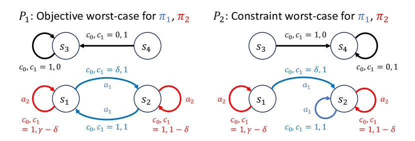
Consider the RCMDP with presented in Figure 1(a) with and set for simplicity. Let and be policies that select and for all states, respectively. For both policies, the objective worst-case is and the constraint worst-case is (see Appendix G). Hence, switching from policy to taking action decreases the objective return under but increases the constraint return under . This conflict causes the gradients of for the objective and for the constraint to sum to a constant vector, i.e.,
showing that is a stationary point. However, cannot solve because would clearly result in a smaller . This stationary point becomes a strict local minimum with a positive , where slightly prefers over (see Appendix G for details).
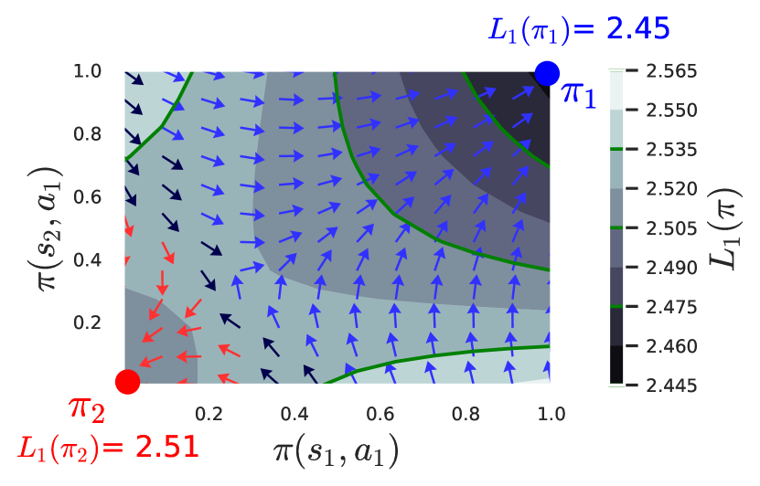
Figure 1(b) computationally illustrates this negative result by plotting the landscape of in the RCMDP example across all possible policies for . We set as does not influence the landscape of . In this example, becomes a local minimum that attracts the policy gradient but fails to solve , as achieves .
This negative result underscores the difficulty of RCMDPs in contrast to CMDPs. In CMDP, where , for any , the problem reduces to solving a standard MDP with a cost function in the environment . As a result, the well-known policy gradient analysis by Agarwal et al. (2021) guarantees that the policy gradient method (Equation 1) converges to stationary points that solve . However, the negative result presented above reveals that there exist RCMDPs where Equation 1 fails by encountering a local minimum.
5 Alternative RCMDP Formulation
This section introduces the epigraph form of RCMDP, which overcomes the challenges discussed in Section 4. For any constrained optimization problem of the form with and , its epigraph form is defined as:
| (6) |
with variables and . It is well-known that is optimal for Equation 6 if and only if is optimal for the original problem and (see, e.g., Boyd & Vandenberghe (2004)).
5.1 Epigraph Form of RCMDP
Based on Equation 6, the RCMDP problem can be equivalently written as:
| (7) |
where we define such that . represents the maximum violation of the constraints of the policy , with the additional constraint . By moving to the constraint, Equation 7 can be further transformed as follows:
Theorem 5.1.
Let . Then,
| (8) |
Furthermore, if , any policy is optimal.
The proof is provided in Section H.2. Instead of Equation 7, we call Equation 8 the epigraph form of RCMDP. Intuitively, the epigraph form seeks the smallest threshold value such that there exists a feasible policy that also satisfies . If , such a feasible policy exists; if , no feasible policy achieves .
Since the epigraph form provides and , the remaining question is whether Equation 8 can be easily solved. To address this, the following properties of are useful:
Lemma 5.2.
is monotonically decreasing in and .
The proof is provided in Section H.1. Given the monotonicity of , if can be efficiently computed, a line search over will readily yield . Increase if , and decrease it if , as illustrated in Figure 2.
5.2 On Computing
To compute , we need to solve the following optimization problem:
| (9) |
Clearly, the right-hand side of Equation 9 is an RMDP problem with added robustness over the set of modified cost functions . Since is neither -rectangular nor -rectangular (see, e.g., Iyengar (2005)), DP approaches are inadequate for this problem. Therefore, we employ the policy gradient method to compute by assuming the following general structure on the uncertainty set:
Assumption 5.3.
is either () a finite set or () a compact set such that, for any , is continuous with respect to .
Then, the subgradient is represented as follows, with the proof provided in Section H.3:
Lemma 5.4.
For any and , define
| (10) |
Let denote the convex hull of a set . Under Assumption 5.3, for any and , the subgradient of at is given by
Here, returns the set , which contains all cost and environment pairs that achieve the worst-case for , while denotes the set of policy gradients corresponding to . Roughly speaking, while involves summing policy gradients from return functions across different environments (see Example 4.2), can focus on the policy gradient of a single worst-case environment by taking . Consequently, avoids the sum of conflicting policy gradients, thereby circumventing the gradient conflict challenge discussed in Section 4.
To formally guarantee that any stationary point of the policy gradient is globally optimal, we introduce the following assumption regarding the coverage of the initial distribution:
Assumption 5.5.
The initial distribution satisfies .
Similar assumptions are used in policy gradient literature for MDPs (Agarwal et al., 2021), CMDPs (Ying et al., 2022), and RMDPs (Wang et al., 2023; Li et al., 2022). Additionally, we remark that the Lagrangian approach performs poorly even under Assumption 5.5 as Theorem 4.1 demonstrates.
Assumption 5.5 allows the epigraph form to enjoy the following gradient-dominance property (see, e.g., Agarwal et al. (2021)), which ensures that any stationary point is globally optimal:
Theorem 5.6 (Gradient dominance).
The detailed proof can be found in Section H.4. Our proof is similar to Theorem 3.2 in Wang et al. (2023), but it is more rigorous and corrects a crucial error that can invalidate their result666For example, their proof around Equation (32) incorrectly bounds a positive value by a negative value.. Moreover, while their proof is limited to cases where is finite, ours is not. We leverage Sion’s minimax theorem (Sion, 1958) for this refinement.
6 Algorithm
This section introduces a double-loop algorithm to solve the epigraph form (Equation 8) using a subroutine algorithm that approximately solves . Throughout this section, we assume access to the following oracle that approximately evaluates the value of .
Assumption 6.1 (Evaluation oracle).
We have an oracle that takes a value and a policy , and returns a value such that , where is an unknown value.
This assumption is mild and easy to meet in practice. For example, if the uncertainty set incorporates a structural assumption like -rectangularity or -rectangularity, this evaluation oracle can be efficiently implemented using robust DP methods (Iyengar, 2005; Kumar et al., 2022; 2024).
Note that solving an RMDP is generally NP-hard when the uncertainty set satisfies only Assumption 5.3 (Wiesemann et al., 2013). The hardness primarily stems from evaluating . Assumption 6.1 mitigates this hardness by abstracting the evaluation step, avoiding the need for additional structural assumptions on .
(also referred to as EpiRC-PGS when using Algorithm 1 as the subroutine)
6.1 Subroutine Algorithm to Solve
The subroutine algorithm updates policies via a policy gradient method. Starting from an arbitrary initial policy , let be the updated policies where is the iteration length.
Recall that , defined in Lemma 5.4, is a subset of the subgradient . We assume access to an oracle that can approximate a subgradient element in .
Assumption 6.2 (Gradient estimator).
Let be an unknown value. We have an oracle that takes a value and a policy , and returns a vector such that .
Similar to Assumption 6.1, this oracle can be efficiently implemented within uncertainty sets with certain structural assumptions (Kumar et al., 2024; Wang & Zou, 2022).
Using the gradient oracle and a learning rate , we update the policy according to the following projected policy gradient, which is similar to Equation 1:
| (11) |
We summarize the pseudocode of the policy gradient procedure in Algorithm 1. The following theorem demonstrates that Algorithm 1 finds a near-minimum point of .
Theorem 6.3.
Suppose Assumptions 5.3, LABEL:, 5.5, LABEL:, 6.1, LABEL: and 6.2 hold. Then, there exist problem-dependent constants that do not depend on such that, when Algorithm 1 is run with and , if the gradient estimation is sufficiently accurate such that , Algorithm 1 returns a policy satisfying
We provide the proof and the concrete values of and in Section I.1.
6.2 Binary Search with Subroutine
Our double-loop algorithm employs a binary search method to solve the epigraph form, supported by a subroutine algorithm that satisfies the following assumption.
Assumption 6.4 (Subroutine algorithm).
We have a subroutine algorithm that takes a value and returns a policy such that with an unknown .
As we have shown in Theorem 6.3, Assumption 6.4 can be realized by Algorithm 1.
Let be the number of iterations of the binary search. For each iteration , let be the search space where . We set and . We denote . Additionally, given , we denote the returned policy from as and its value evaluated by as .
Our binary search aims to identify the minimum such that , as such satisfies . Following the strategy illustrated in Figure 2, we increase if ; otherwise, we decrease it. More concretely, our binary search iteratively narrows down the search space as follows:
| (12) |
We summarize the pseudocode of the algorithm in Algorithm 2. The following Theorem 6.5 ensures that Algorithm 2 returns a near-optimal policy. We provide the proof in Section I.2.
Theorem 6.5.
Suppose that Algorithm 2 is run with oracles and that satisfy Assumptions 6.1, LABEL: and 6.4. Then, Algorithm 2 returns an -optimal policy, where .
We refer to Algorithm 2 with Algorithm 1 subroutine as Epigraph Robust Constrained Policy Gradient Search (EpiRC-PGS). By applying Theorem 6.3 to Theorem 6.5, the following corollary shows that EpiRC-PGS finds an -optimal policy by making queries to the oracles and .
Corollary 6.6.
Assume Assumptions 5.3, LABEL: and 5.5 holds. Suppose we have sufficiently accurate oracles and that satisfy Assumption 6.1 and Assumption 6.2 with and , respectively. Set Algorithm 1 as the subroutine algorithm with parameters , where we set , , using and from Theorem 6.3. Then, given inputs and , Algorithm 2 returns an -optimal policy after iteration.
Finally, we remark that EpiRC-PGS converges in a last-iterate sense. While many Lagrangian-based algorithms for CMDPs provide certain performance guarantees for the average of past policies (Miryoosefi et al., 2019; Chen et al., 2021; Li et al., 2021; Liu et al., 2021), they become problematic in scenarios where policy averaging is impractical, such as in deep RL. In contrast, Corollary 6.6 does not require policy averaging and ensures that the final policy output is near-optimal.
7 Experiments
This section empirically compares our EpiRC-PGS algorithm to a Lagrangian counterpart, which aims to solve the problem in Equation 4 by performing gradient ascent on while using a policy gradient subroutine to solve . We refer to this Lagrangian-based algorithm as the “Lagrangian Formulation Policy Gradient Search (LF-PGS).” LF-PGS abstracts some existing Lagrangian-based algorithms for RCMDPs (e.g., (Russel et al., 2020; Wang et al., 2022)). The detailed implementation of LF-PGS is provided in Appendix B.
Since Lagrangian-based algorithms typically require averaging the optimization variables obtained during updates (Miryoosefi et al., 2019; Chen et al., 2021; Li et al., 2021; Liu et al., 2021), we also report the performance of the averaged policies from LF-PGS, where the -th policy is set as . We refer to this averaging algorithm as LF-PGS-avg.
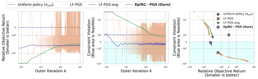
Figure 3 shows the objective return and constraint violation for algorithms averaged over 20 randomly generated simple RCMDPs with finite uncertainty sets. The details of the environmental setup are provided in Appendix B. For each -th outer iteration, we report the objective return minus the return of the uniform policy, i.e., , where represents a uniform policy. This subtraction accounts for variations in the minimum return across different RCMDPs.
Results.
The left and middle figures in Figure 3 demonstrate that EpiRC-PGS rapidly converges to a policy that not only satisfies the constraints but also achieves a low objective return. In contrast, LF-PGS exhibits oscillatory returns and constraint violations. Even when averaging its policies (LF-PGS-avg), the objective return remains worse than EpiRC-PGS and continues to exhibit constraint violations, indicating suboptimal performance. Additionally, the right figure of Figure 3 reveals that any other algorithm does not find the feasible and low-return policy identified by EpiRC-PGS ( ● in the figure). These findings empirically validate that EpiRC-PGS yields a near-optimal policy, contrasting with the conventional Lagrangian-based algorithm’s inability to do so.
8 Conclusion and Limitations
In this work, we propose EpiRC-PGS, the first algorithm guaranteed to find a near-optimal policy in an RCMDP (Corollary 6.6). At the core of EpiRC-PGS is the use of the epigraph form for RCMDP. Remarkably, the epigraph form produces the optimal policy (Section 5.1) and supports a policy gradient algorithm to find it (Section 5.2). These features effectively address the optimization challenges encountered in the conventional Lagrangian formulation (Section 4).
Limitations and future work.
A double-loop algorithm like EpiRC-PGS is often impractical when the inner problem requires high computational cost (Lin et al., 2024). Developing a single-loop algorithm based on the epigraph form is a promising direction for future research. To support future RCMDP studies, we discuss the potential difficulty in designing such an algorithm in Appendix C.
Another area for future research involves improving iteration complexity. It is known that with a rectangularity assumption, the natural policy gradient method can find an -optimal policy in RMDP with iterations Li et al. (2022). Investigating whether our complexity in RCMDP can be improved is a promising area for future research.
Finally, we leave for future work the exploration of removing the coverage assumption on the initial distribution (Assumption 5.5). Although this assumption can be readily satisfied in robust policy design using simulators by assigning negligible initial probabilities to all states, it may violate the theoretical guarantees of the designed policy, as optimal policies in CMDP depend on the initial state distribution (Altman, 1999).
References
- Abernethy & Wang (2017) Jacob D Abernethy and Jun-Kun Wang. On Frank-Wolfe and Equilibrium Computation. In Advances in Neural Information Processing Systems, 2017.
- Achiam et al. (2017) Joshua Achiam, David Held, Aviv Tamar, and Pieter Abbeel. Constrained Policy Optimization. In International Conference on Machine Learning, 2017.
- Agarwal et al. (2021) Alekh Agarwal, Sham M Kakade, Jason D Lee, and Gaurav Mahajan. On the Theory of Policy Gradient Methods: Optimality, Approximation, and Distribution Shift. Journal of Machine Learning Research, 22(98):1–76, 2021.
- Altman (1999) Eitan Altman. Constrained Markov Decision Processes, volume 7. CRC Press, 1999.
- Anderson et al. (2019) James Anderson, John C Doyle, Steven H Low, and Nikolai Matni. System Level Synthesis. Annual Reviews in Control, 47:364–393, 2019.
- Bellman et al. (1957) R. Bellman, R.E. Bellman, and Rand Corporation. Dynamic Programming. Princeton University Press, 1957.
- Bemporad & Morari (2007) Alberto Bemporad and Manfred Morari. Robust Model Predictive Control: A Survey. In Robustness in Identification and Control, pp. 207–226. Springer, 2007.
- Beyer & Sendhoff (2007) Hans-Georg Beyer and Bernhard Sendhoff. Robust Optimization–a Comprehensive Survey. Computer Methods in Applied Mechanics and Engineering, 196(33-34):3190–3218, 2007.
- Bhandari & Russo (2024) Jalaj Bhandari and Daniel Russo. Global Optimality Guarantees for Policy Gradient Methods. Operations Research, 2024.
- Borkar (1988) Vivek S Borkar. A convex analytic approach to Markov Decision Processes. Probability Theory and Related Fields, 78(4):583–602, 1988.
- Boyd & Vandenberghe (2004) Stephen P Boyd and Lieven Vandenberghe. Convex Optimization. Cambridge University Press, 2004.
- Bura et al. (2022) Archana Bura, Aria HasanzadeZonuzy, Dileep Kalathil, Srinivas Shakkottai, and Jean-Francois Chamberland. DOPE: Doubly Optimistic and Pessimistic Exploration for Safe Reinforcement Learning. In Advances in Neural Information Processing Systems, 2022.
- Chang (2023) Hyeong Soo Chang. Approximate Constrained Discounted Dynamic Programming with Uniform Feasibility and Optimality. arXiv preprint arXiv:2308.03297, 2023.
- Chen & Blankenship (2004) Richard C Chen and Gilmer L Blankenship. Dynamic Programming Equations for Discounted Constrained Stochastic Control. IEEE Transactions on Automatic Control, 49(5):699–709, 2004.
- Chen & Feinberg (2006) Richard C Chen and Eugene A Feinberg. Non-Randomized Control of Constrained Markov Decision Processes. In American Control Conference, 2006.
- Chen et al. (2021) Yi Chen, Jing Dong, and Zhaoran Wang. A Primal-Dual Approach to Constrained Markov Decision Processes. arXiv preprint arXiv:2101.10895, 2021.
- Clarke et al. (2008) Francis H Clarke, Yuri S Ledyaev, Ronald J Stern, and Peter R Wolenski. Nonsmooth analysis and Control Theory, volume 178. Springer Science & Business Media, 2008.
- Clavier et al. (2023) Pierre Clavier, Erwan Le Pennec, and Matthieu Geist. Towards minimax Optimality of Model-based Robust Reinforcement Learning. arXiv preprint arXiv:2302.05372, 2023.
- Dann et al. (2017) Christoph Dann, Tor Lattimore, and Emma Brunskill. Unifying PAC and Regret: Uniform PAC Bounds for Episodic Reinforcement Learning. In Advances in Neural Information Processing Systems, 2017.
- Denardo (1970) Eric V Denardo. On Linear Programming in a Markov Decision Problem. Management Science, 16(5):281–288, 1970.
- Derman et al. (2021) Esther Derman, Matthieu Geist, and Shie Mannor. Twice Regularized MDPs and the Equivalence Between Robustness and Regularization. Advances in Neural Information Processing Systems, 34:22274–22287, 2021.
- Ding et al. (2020) Dongsheng Ding, Kaiqing Zhang, Tamer Basar, and Mihailo Jovanovic. Natural Policy Gradient Primal-Dual Method for Constrained Markov Decision Processes. In Advances in Neural Information Processing Systems, 2020.
- Ding et al. (2023) Dongsheng Ding, Chen-Yu Wei, Kaiqing Zhang, and Alejandro Ribeiro. Last-Iterate Convergent Policy Gradient Primal-Dual Methods for Constrained MDPs. arXiv preprint arXiv:2306.11700, 2023.
- Doyle (1982) John Doyle. Analysis of Feedback Systems with Structured Uncertainties. In IEE Proceedings D-Control Theory and Applications, 1982.
- Du et al. (2021) Simon Du, Sham Kakade, Jason Lee, Shachar Lovett, Gaurav Mahajan, Wen Sun, and Ruosong Wang. Bilinear Classes: A Structural Framework for Provable Generalization in RL. In International Conference on Machine Learning, 2021.
- Du et al. (2018) Simon S Du, Yining Wang, Sivaraman Balakrishnan, Pradeep Ravikumar, and Aarti Singh. Robust Nonparametric Regression under Huber’s -contamination Model. arXiv preprint arXiv:1805.10406, 2018.
- Efroni et al. (2020) Yonathan Efroni, Shie Mannor, and Matteo Pirotta. Exploration-Exploitation in Constrained MDPs. arXiv preprint arXiv:2003.02189, 2020.
- Ghosh (2024) Arnob Ghosh. Sample Complexity for Obtaining Sub-optimality and Violation Bound for Distributionally Robust Constrained MDP. In Reinforcement Learning Safety Workshop, 2024.
- Goyal & Grand-Clement (2023) Vineet Goyal and Julien Grand-Clement. Robust Markov Decision Processes: Beyond Rectangularity. Mathematics of Operations Research, 48(1):203–226, 2023.
- Grand-Clément & Kroer (2021) Julien Grand-Clément and Christian Kroer. Scalable First-Order Methods for Robust Mdps. In AAAI Conference on Artificial Intelligence, volume 35, pp. 12086–12094, 2021.
- Grand-Clément & Petrik (2022) Julien Grand-Clément and Marek Petrik. On the Convex Formulations of Robust Markov Decision Processes. arXiv preprint arXiv:2209.10187, 2022.
- HasanzadeZonuzy et al. (2021) Aria HasanzadeZonuzy, Archana Bura, Dileep Kalathil, and Srinivas Shakkottai. Learning with Safety Constraints: Sample Complexity of Reinforcement Learning for Constrained MDPs. In AAAI Conference on Artificial Intelligence, 2021.
- Haviv (1996) Moshe Haviv. On Constrained Markov Decision Processes. Operations Research Letters, 19(1):25–28, 1996.
- Iyengar (2005) Garud N Iyengar. Robust Dynamic Programming. Mathematics of Operations Research, 30(2):257–280, 2005.
- Jiang (2018) Nan Jiang. PAC Reinforcement Learning with an Imperfect Model. In AAAI Conference on Artificial Intelligence, volume 32, 2018.
- Kitamura et al. (2024) Toshinori Kitamura, Tadashi Kozuno, Masahiro Kato, Yuki Ichihara, Soichiro Nishimori, Akiyoshi Sannai, Sho Sonoda, Wataru Kumagai, and Yutaka Matsuo. A Policy Gradient Primal-Dual Algorithm for Constrained MDPs with Uniform PAC Guarantees. arXiv preprint arXiv:2401.17780, 2024.
- Kruger (2003) A Ya Kruger. On Fréchet Subdifferentials. Journal of Mathematical Sciences, 116(3):3325–3358, 2003.
- Kumar et al. (2022) Navdeep Kumar, Kfir Levy, Kaixin Wang, and Shie Mannor. Efficient Policy Iteration for Robust Markov Decision Processes via Regularization. arXiv preprint arXiv:2205.14327, 2022.
- Kumar et al. (2024) Navdeep Kumar, Esther Derman, Matthieu Geist, Kfir Y Levy, and Shie Mannor. Policy Gradient for Rectangular Robust Markov Decision Processes. Advances in Neural Information Processing Systems, 36, 2024.
- Le et al. (2019) Hoang Le, Cameron Voloshin, and Yisong Yue. Batch Policy Learning Under Constraints. In International Conference on Machine Learning, 2019.
- Li et al. (2021) Tianjiao Li, Ziwei Guan, Shaofeng Zou, Tengyu Xu, Yingbin Liang, and Guanghui Lan. Faster Algorithm and Sharper Analysis for Constrained Markov Decision Process. arXiv preprint arXiv:2110.10351, 2021.
- Li et al. (2022) Yan Li, Guanghui Lan, and Tuo Zhao. First-Order Policy Optimization for Robust Markov Decision Process. arXiv preprint arXiv:2209.10579, 2022.
- Lin et al. (2024) Zhenwei Lin, Chenyu Xue, Qi Deng, and Yinyu Ye. A Single-Loop Robust Policy Gradient Method for Robust Markov Decision Processes. arXiv preprint arXiv:2406.00274, 2024.
- Liu et al. (2021) Tao Liu, Ruida Zhou, Dileep Kalathil, Panganamala Kumar, and Chao Tian. Learning Policies with Zero or Bounded Constraint Violation for Constrained MDPs. In Advances in Neural Information Processing Systems, 2021.
- Mai & Jaillet (2021) Tien Mai and Patrick Jaillet. Robust Entropy-Regularized Markov Decision Processes. arXiv preprint arXiv:2112.15364, 2021.
- Mankowitz et al. (2020) Daniel J Mankowitz, Dan A Calian, Rae Jeong, Cosmin Paduraru, Nicolas Heess, Sumanth Dathathri, Martin Riedmiller, and Timothy Mann. Robust Constrained Reinforcement Learning for Continuous Control with Model Misspecification. arXiv preprint arXiv:2010.10644, 2020.
- Mikhalevich et al. (2024) VS Mikhalevich, AM Gupal, and VI Norkin. Methods of Nonconvex Optimization. arXiv preprint arXiv:2406.10406, 2024.
- Miryoosefi et al. (2019) Sobhan Miryoosefi, Kianté Brantley, Hal Daume III, Miro Dudik, and Robert E Schapire. Reinforcement Learning with Convex Constraints. In Advances in Neural Information Processing Systems, 2019.
- Mnih et al. (2015) Volodymyr Mnih, Koray Kavukcuoglu, David Silver, Andrei A Rusu, Joel Veness, Marc G Bellemare, Alex Graves, Martin Riedmiller, Andreas K Fidjeland, Georg Ostrovski, et al. Human-level Control through Deep Reinforcement Learning. Nature, 518(7540):529–533, 2015.
- Moskovitz et al. (2023) Ted Moskovitz, Brendan O’Donoghue, Vivek Veeriah, Sebastian Flennerhag, Satinder Singh, and Tom Zahavy. ReLOAD: Reinforcement Learning with Optimistic Ascent-Descent for Last-Iterate Convergence in Constrained MDPs. In International Conference on Machine Learning, 2023.
- Müller et al. (2024) Adrian Müller, Pragnya Alatur, Volkan Cevher, Giorgia Ramponi, and Niao He. Truly No-Regret Learning in Constrained MDPs. arXiv preprint arXiv:2402.15776, 2024.
- Nachum & Dai (2020) Ofir Nachum and Bo Dai. Reinforcement Learning via Fenchel-Rockafellar Duality. arXiv preprint arXiv:2001.01866, 2020.
- Nilim & El Ghaoui (2005) Arnab Nilim and Laurent El Ghaoui. Robust Control of Markov Decision Processes with Uncertain Transition Matrices. Operations Research, 53(5):780–798, 2005.
- Panaganti & Kalathil (2022) Kishan Panaganti and Dileep Kalathil. Sample Complexity of Robust Reinforcement Learning with a Generative Model. In International Conference on Artificial Intelligence and Statistics, 2022.
- Parikh et al. (2014) Neal Parikh, Stephen Boyd, et al. Proximal algorithms. Foundations and Trends® in Optimization, 1(3):127–239, 2014.
- Paternain et al. (2019) Santiago Paternain, Luiz Chamon, Miguel Calvo-Fullana, and Alejandro Ribeiro. Constrained Reinforcement Learning Has Zero Duality Gap. In Advances in Neural Information Processing Systems, 2019.
- Paternain et al. (2022) Santiago Paternain, Miguel Calvo-Fullana, Luiz FO Chamon, and Alejandro Ribeiro. Safe Policies for Reinforcement Learning via Primal-Dual Methods. IEEE Transactions on Automatic Control, 2022.
- Rahimian & Mehrotra (2019) Hamed Rahimian and Sanjay Mehrotra. Distributionally Robust Optimization: A Review. arXiv preprint arXiv:1908.05659, 2019.
- Rockafellar & Wets (2009) R Tyrrell Rockafellar and Roger J-B Wets. Variational Analysis, volume 317. Springer Science & Business Media, 2009.
- Russel et al. (2020) Reazul Hasan Russel, Mouhacine Benosman, and Jeroen Van Baar. Robust Constrained-MDPs: Soft-constrained Robust Policy Optimization under Model Uncertainty. arXiv preprint arXiv:2010.04870, 2020.
- Sion (1958) Maurice Sion. On General Minimax Theorems. Pacific Journal of Mathematics, 8(1):171 – 176, 1958.
- Sun et al. (2024) Zhongchang Sun, Sihong He, Fei Miao, and Shaofeng Zou. Constrained Reinforcement Learning Under Model Mismatch. arXiv preprint arXiv:2405.01327, 2024.
- Taguchi et al. (1986) G. Taguchi, G. Taguchi, and Asian Productivity Organization. Introduction to Quality Engineering: Designing Quality Into Products and Processes. Asian Productivity Organization, 1986.
- Tessler et al. (2018) Chen Tessler, Daniel J Mankowitz, and Shie Mannor. Reward Constrained Policy Optimization. In International Conference on Learning Representations, 2018.
- Wang et al. (2023) Qiuhao Wang, Chin Pang Ho, and Marek Petrik. Policy Gradient in Robust MDPs with Global Convergence Guarantee. In International Conference on Machine Learning, 2023.
- Wang & Zou (2021) Yue Wang and Shaofeng Zou. Online Robust Reinforcement Learning with Model Uncertainty. In Advances in Neural Information Processing Systems, 2021.
- Wang & Zou (2022) Yue Wang and Shaofeng Zou. Policy Gradient Method for Robust Reinforcement Learning. In International Conference on Machine Learning, 2022.
- Wang et al. (2022) Yue Wang, Fei Miao, and Shaofeng Zou. Robust Constrained Reinforcement Learning. arXiv preprint arXiv:2209.06866, 2022.
- Wei et al. (2021) Honghao Wei, Xin Liu, and Lei Ying. A Provably-Efficient Model-Free Algorithm for Constrained Markov Decision Processes. arXiv preprint arXiv:2106.01577, 2021.
- Wiesemann et al. (2013) Wolfram Wiesemann, Daniel Kuhn, and Berç Rustem. Robust Markov Decision Processes. Mathematics of Operations Research, 38(1):153–183, 2013.
- Yang et al. (2023) Wenhao Yang, Han Wang, Tadashi Kozuno, Scott M Jordan, and Zhihua Zhang. Robust Markov Decision Processes without Model Estimation. arXiv preprint arXiv:2302.01248, 2023.
- Ying et al. (2022) Donghao Ying, Yuhao Ding, and Javad Lavaei. A Dual Approach to Constrained Markov Decision Processes with Entropy Regularization. In International Conference on Artificial Intelligence and Statistics, 2022.
- Zahavy et al. (2021) Tom Zahavy, Brendan O’Donoghue, Guillaume Desjardins, and Satinder Singh. Reward is Enough for Convex MDPs. In Advances in Neural Information Processing Systems, 2021.
- Zames (1981) George Zames. Feedback and Optimal Sensitivity: Model Reference Transformations, Multiplicative Seminorms, and Approximate Inverses. IEEE Transactions on Automatic Control, 26(2):301–320, 1981.
- Zhang et al. (2024) Zhengfei Zhang, Kishan Panaganti, Laixi Shi, Yanan Sui, Adam Wierman, and Yisong Yue. Distributionally Robust Constrained Reinforcement Learning under Strong Duality. arXiv preprint arXiv:2406.15788, 2024.
- Zheng & Ratliff (2020) Liyuan Zheng and Lillian Ratliff. Constrained Upper Confidence Reinforcement Learning. In Learning for Dynamics and Control, 2020.
Appendix A Additional Related Work
This section reviews existing approaches for CMDPs and RMDPs. It also highlights their inherent limitations and the challenges they face when applied to RCMDPs.
A.1 Constrained Markov Decision Processes
CMDP is a specific subclass of RCMDP where the uncertainty set consists of a single element, i.e., . This section describes two primary approaches to the CMDP problem: the linear programming (LP) approach and the Lagrangian approach.
Linear programming approach.
The LP approach has been extensively studied in the theoretical literature (Efroni et al., 2020; Liu et al., 2021; Bura et al., 2022; HasanzadeZonuzy et al., 2021; Zheng & Ratliff, 2020). Although it is a fundamental method in CMDP, it is less popular in practice due to its difficulty in scaling to high-dimensional problem settings, such as those encountered in deep RL. Additionally, incorporating environmental uncertainty into the LP approach for CMDPs is challenging. The LP approach utilizes the fact that the return minimization problem of an MDP can be formulated as a convex optimization problem with respect to the occupancy measure (Altman, 1999; Nachum & Dai, 2020). However, RMDPs do not permit a convex formulation in terms of occupancy measures (Iyengar, 2005; Grand-Clément & Petrik, 2022). While Grand-Clément & Petrik (2022) recently introduced a convex optimization approach for RMDPs, their formulation is convex for the transformed objective value function, not for the occupancy measure, making it challenging to incorporate constraints as seen in RCMDPs.
Lagrangian approach.
The Lagrangian approach is perhaps the most popular approach to CMDPs both in theory (Ding et al., 2020; Wei et al., 2021; HasanzadeZonuzy et al., 2021; Kitamura et al., 2024) and practice (Achiam et al., 2017; Tessler et al., 2018; Wang et al., 2022; Le et al., 2019; Russel et al., 2020). This popularity stems from its compatibility with policy gradient methods, making it readily extendable to deep RL. The Lagrangian approach benefits from the strong duality in CMDPs. When consists of a single element, it is well established that strong duality holds, meaning that holds, where is from Equation 4 and is from Equation 2 (Altman, 1999; Paternain et al., 2019; 2022).
The challenge with the Lagrangian method is the identification of an optimal policy. Even if Equation 4 is solved, there’s no guarantee that the solution to the inner minimization problem will represent an optimal policy. In some CMDPs, where feasible policies in must be stochastic (Altman, 1999), the inner minimization may yield a deterministic solution that is infeasible. Zahavy et al. (2021); Miryoosefi et al. (2019); Chen et al. (2021); Li et al. (2021); Liu et al. (2021) addressed this challenge by averaging policies (or occupancy measures) obtained during the optimization process. However, policy averaging can be impractical for large-scale algorithms (e.g., deep RL) because it necessitates storing all past policies, which is often infeasible. On the other hand, Ying et al. (2022); Ding et al. (2023); Müller et al. (2024); Kitamura et al. (2024) tackled the issue by introducing entropy regularization into the objective return. However, the regularization can lead to biased solutions and result in a policy design that may deviate from what is intended by the cost function.
In contrast, EpiRC-PGS requires neither policy averaging nor regularization, thereby offering advantageous properties even in CMDP settings.
A.2 Robust Markov Decision Processes
RMDP is a specific subclass of RCMDP where there are no constraints, i.e., . RMDP is a crucial research area for the practical success of RL applications, where the environmental mismatch between the training phase and the testing phase is almost unavoidable. Without robust policy design, even a small mismatch can lead to poor performance of the trained policy in the testing phase (Li et al., 2022; Jiang, 2018).
Dynamic programming approach.
Since the seminal work by Iyengar (2005), numerous studies have explored dynamic programming (DP) approaches for RMDPs (Nilim & El Ghaoui, 2005; Clavier et al., 2023; Panaganti & Kalathil, 2022; Mai & Jaillet, 2021; Grand-Clément & Kroer, 2021; Derman et al., 2021; Wang & Zou, 2021; Kumar et al., 2022; Yang et al., 2023). The DP approach decomposes the original problem into smaller sub-problems using Bellman’s principle of optimality (Bellman et al., 1957). To apply this principle, DP approaches enforce rectangularity on the uncertainty set, which assumes independent worst-case transitions at each state or state-action pair. However, as pointed out by Goyal & Grand-Clement (2023), the rectangularity assumption can result in a very conservative optimal policy. Moreover, applying DP to constrained settings is challenging since CMDPs typically do not satisfy the principle of optimality (Haviv, 1996). Although several studies have attempted to apply DP to CMDPs, they face issues such as excessive memory consumption, due to the use of non-stationary policy classes, or are restricted to deterministic policy classes (Chang, 2023; Chen & Blankenship, 2004; Chen & Feinberg, 2006).
Policy gradient approach.
Another promising approach for RMDPs is the policy gradient method. Similar to the DP approach, most existing policy gradient algorithms also work only under the rectangularity assumption (Kumar et al., 2024; Wang & Zou, 2022; Li et al., 2022), and thus suffer from the same conservativeness issue. It is important to note that robust policy evaluation can be NP-hard without any structural assumptions on the uncertainty set (Wiesemann et al., 2013), but such assumptions are potentially not required for the robust policy optimization step. Our policy gradient algorithm abstracts the evaluation step by Assumption 6.1 and avoids the need for the rectangularity assumption during the policy optimization phase, similar to the recent work by Wang et al. (2023).
A.3 Notes on the Policy-Mixing Technique
This section explains the theoretical limitations of the policy-mixing technique (Zhang et al., 2024; Miryoosefi et al., 2019; Le et al., 2019) for identifying a near-optimal policy.
Policy-mixing technique.
Let be a finite set of policies with . Consider a non-robust, single-constraint CMDP . Given a distribution , define
The policy-mixing technique considers the following optimization problem:
| (13) | ||||
Let be the solution of Equation 13 such that .
In this setting, a policy is sampled from at the start of each episode and remains fixed throughout the episode. The term represents the expected return under the distribution . Since is convex in and concave in , under some mild assumptions, Equation 13 can be solved efficiently by the following standard optimization procedure for min-max problems: At each iteration , with initial values and ,
-
1.
Update using a no-regret algorithm. For example, with gradient ascent and a learning rate :
-
2.
Update as where
Then, the averaged distribution converges to as (Abernethy & Wang, 2017; Zahavy et al., 2021). When is sufficiently large, we can expect that the optimal value of Equation 13 is equivalent to that of the CMDP problem, i.e., , where is defined in Equation 2 with .
Limitation of policy-mixing.
Even when , it is crucial to note that, while converges to , there is no guarantee that will converge to .
Let . Zhang et al. (2024); Miryoosefi et al. (2019); Le et al. (2019) argued for the convergence of by asserting that the equality (a) in the following equation holds:
| (14) | ||||
(see, for example, Equation (14) in Zhang et al. (2024), Equation (1) in Le et al. (2019), and around Equation (13) in Miryoosefi et al. (2019)).
However, (a) in Equation 14 does not hold in general because the return function is neither convex nor concave in policy. Even when , there is an example where Equation 14 fails (see Proof of Lemma 3.1 in Agarwal et al. (2021)). This invalidates the results of Miryoosefi et al. (2019); Le et al. (2019); Zhang et al. (2024), thus illustrating the theoretical limitations of the policy-mixing approach for near-optimal policy identification.
Appendix B Experiment Details
The source code for the experiment is available at https://github.com/matsuolab/RCMDP-Epigraph.
Environment construction.
We conduct the experiment on randomly generated simple RCMDP instances, whose uncertainty set is finite with . We employ a construction strategy similar to that of Dann et al. (2017). Each transition kernel is randomly instantiated. For all , the transition probabilities are independently sampled from . This transition probability kernel is concentrated yet encompasses non-deterministic transition probabilities.
The parameters are set as follows: , , , and . The cost values for the objective are set to with probability and are uniformly chosen at random from otherwise. The cost values for the constraint are set to . Thus, the constraint and objective are in conflict in this CMDP. This aligns with the CMDP construction strategy proposed by Moskovitz et al. (2023) to generate a hard CMDP instance.
The initial state probabilities are independently sampled from . The constraint threshold is set so that the uniform policy violates the threshold while ensuring that a feasible policy does exist.
EpiRC-PGS implementation.
For the policy gradient subroutine (Algorithm 1), we set the iteration length to and the learning rate to . These values are selected to ensure that Assumption 6.1 is satisfied with a sufficiently small . Since the initial policy in Algorithm 1 can be chosen arbitrarily, the -th policy from the outer loop is used as the initial policy for the -th policy computation.
LF-PGS implementation.
The pseudocode for LF-PGS is shown in Algorithm 3. We set the iteration length and learning rate for the inner policy optimization to and . Similar to EpiRC-PGS, these values are chosen to ensure sufficiently accurate optimization in the inner loop. After a hyperparameter tuning, we choose for the outer updates, balancing between the convergence speed and performance.
Appendix C Discussion on Single-Loop Algorithm
Although Algorithm 2 can identify a near-optimal policy, it uses a double-loop structure that repetitively solves by Algorithm 1. In practice, single-loop algorithms, such as primal-dual algorithms for CMDPs (e.g., Efroni et al. (2020); Ding et al. (2023)), are typically more efficient and preferable compared to double-loop algorithms. This section discusses the challenge of designing a single-loop algorithm for the epigraph form.
Since the epigraph form is a constrained optimization problem, we can further transform it using a Lagrangian multiplier , yielding:
| (15) |
Similar to the typical Lagrangian approach, let’s swap the min-max order. We call the resulting formulation the “epigraph-Lagrange” formulation:
| (16) |
Does the strong duality, , hold? If it does, we could design a single-loop algorithm similar to primal-dual CMDP algorithms, performing gradient ascent and descent on Equation 16. Unfortunately, proving the strong duality is challenging.
Essentially, the min-max can be swapped when in Equation 15 is quasiconvex-quasiconcave (Sion, 1958). While is clearly concave in , the quasiconvexity in is not obvious. Although is decreasing due to Lemma 5.2 and thus a quasi-convex function, there is no guarantee on the quasi-convexity of . The situation would be resolved if were convex in . However, since is a pointwise minimum and may not be convex in (Agarwal et al., 2021), may not be convex in (Boyd & Vandenberghe, 2004).
Therefore, algorithms for the epigraph-Lagrange formulation face a problem similar to the strong duality challenge of the Lagrangian formulation (Section 4). Proving strong duality or finding alternative ways to circumvent this challenge is a promising direction for future RCMDP research.
Appendix D Additional definitions
Throughout this section, let denote a set such that with .
Definition D.1 (Subgradient (Kruger, 2003)).
Let be an open set where . The (Fréchet) subgradient of a function at a point is defined as the set
Furthermore, if is a singleton, its element is denoted as and called the (Fréchet) gradient of at .
Definition D.2 (Lipschitz continuity).
Let . A function is -Lipschitz if for any , we have that
Definition D.3 (Smoothness).
Let . A function is -smooth if for any , we have that
Definition D.4 (Weak convexity).
Let . A function is -weakly convex if for any and ,
Note that is convex in if and only if is -weakly convex.
Definition D.5 (Moreau envelope of a weakly convex function).
Given a -weakly convex function and a parameter , the Moreau envelope function of is given by such that
Appendix E Useful Lemmas
Throughout this section, denotes a compact set such that , where .
Lemma E.1 (Lemma D.2. in Wang et al. (2023)).
Let and be an -smooth function. Then, is a -weakly convex function.
Lemma E.2 (e.g., Proposition 13.37 in Rockafellar & Wets (2009)).
Let be an -weakly convex function, and let be a parameter. The Moreau envelope function is differentiable, and its gradient is given by
Lemma E.3 (Sion’s minimax theorem (Sion, 1958)).
Let . Let be a compact convex set and a convex set. Suppose that satisfies the following two properties:
-
•
is upper semicontinuous and quasi-concave on for any .
-
•
is lower semicontinuous and quasi-convex on for any .
Then, .
Lemma E.4 (e.g., Problem 9.13, Page 99 in Clarke et al. (2008)).
Let be a compact set and be a continuous function of two arguments. Consider a point and let be its neighborhood. For any , suppose that the gradient exists and is jointly continuous.
Let . Then, the subgradient of at is given by
Lemma E.5.
Let . Let for be -weakly convex functions for some . Define the pointwise maximum function as
Then, for any ,
Proof.
The claim directly follows from Theorem 1.3 and Theorem 1.5 in Mikhalevich et al. (2024). ∎
Lemma E.6 (Maximum difference inequality).
Let . For two sets of real numbers and , where ,
Proof.
For any ,
By the symmetry of and , we have . Therefore,
∎
Lemma E.7 (Point-wise maximum preserves weak convexity).
Let and be - and -weakly convex functions, respectively. Then, defined by for any is -weakly convex, where .
Proof.
By the definition of weak convexity, for any and ,
A similar inequality holds for . Then,
Therefore, is -weakly convex. ∎
Lemma E.8.
Let be the normal cone of at , defined as
Define the indicator function such that
Then, for any .
Proof.
Note that any satisfies
| (17) |
Suppose that . Then, there exists such that , which contradicts Equation 17. Therefore, for any and thus .
Consider . It satisfies for any . Since and by the definition of , Equation 17 holds for any . Therefore, . This concludes the proof. ∎
Lemma E.9.
Let be an -weakly convex function. For , define
Then, there exists a subgradient such that, for any ,
Proof.
Let be a function such that .
Note that
It is clear that is a minimizer of the function . Therefore, it holds that . Accordingly,
Lemma E.10 (Linear optimization on convex hull).
Given and a compact set , it holds that
Proof.
Let . The claim holds for . Suppose that . Then, by the definition of the convex hull, there exist and such that and
Since is a minimizer, we have
Accordingly,
The inequality must be an equality, and thus
Since , it holds that
The above equality means that both and satisfy . Therefore, . ∎
Appendix F Useful Lemmas for MDPs
Lemma F.1 (Lemma 3.1 in Wang et al. (2023)).
Appendix G Proof of Theorem 4.1
Proof of Theorem 4.1.
Consider the deterministic RCMDP shown in Figure 1(a) with , , , and . Set the initial distribution such that .
First part of Theorem 4.1.
Set . The threshold can be arbitrary.
Let and be two policies such that always chooses and always chooses in any state. For any , we will show two results:
-
•
Equation 19: .
-
•
Equation 21: .
The former shows the suboptimality of , and the latter indicates that is a local minimum.
According to the RCMDP construction, for any , we have
For and , it is easy to verify that
Therefore,
| (18) | ||||
Hence,
Accordingly, since , we have
| (19) |
The next task is to show that .
Therefore, since ,
| (21) | ||||
Now, with a sufficiently small , let be policies near . When is sufficiently small, due to the Lipshictz continuity of by Lemma F.1, Equation 18 indicates that
| (22) |
Similarly, due to Equation 22 with the Lipshictz continuity of by Lemma F.1, Equation 20 and Equation 21 indicate that,
Therefore, since always chooses , we have for a sufficiently small . The first part of the claim holds by setting with Equation 19.
Second part of Theorem 4.1.
Consider again the deterministic RCMDP given in the previous part of the proof with . For a value , define a function such that
Appendix H Missing Proofs in Section 5
H.1 Proofs of Lemma 5.2
Proof of Lemma 5.2.
We prove the first claim. Recall the definition of :
| (24) |
It is easy to see that is monotonically decreasing in . Consider two real numbers and let . Then,
Therefore, is monotonically decreasing in .
Next, we prove the second claim. Suppose that . Then, there exists a feasible policy such that . This contradicts the definition of the optimal policy. Therefore, .
Suppose that . Since , no feasible policy achieves the objective return . This also contradicts the existence of the optimal policy. Therefore, . ∎
H.2 Proofs of Theorem 5.1
Proof of Theorem 5.1.
We first prove Equation 8 by contradiction. Let and suppose that . Since by Lemma 5.2, there exists a feasible policy such that . This contradicts the definition of the optimal policy.
We then show that Equation 8 provides . Since by Lemma 5.2, any policy is feasible and satisfies . The claim directly follows from the definition of an optimal policy. ∎
H.3 Proofs of Lemma 5.4
Lemma H.1 (Properties of ).
The following properties hold for any .
-
1.
(Lipschitz continuity): For any , with .
-
2.
(Weak convexity): is convex in with .
-
3.
(Subdifferentiability): For any , the subgradient of at is given by
where represents the convex hull of a set .
Proof of Lipschitz continuity.
Proof of weak convexity.
H.4 Proof of Theorem 5.6
Proof of Theorem 5.6.
Recall that, and defined in Equation 10, are given by:
| (25) |
For simplicity, this proof uses the shorthand and .
The claim holds by showing that
| (27) |
Since due to Lemma H.1, Equation 27 holds when there exists a such that .
Let . For any , it holds that
| (28) | ||||
where (a) uses Sion’s minimax theorem (Lemma E.3) with the convexity of and , and (b) uses Lemma E.10.
Note that
| (29) |
where (a) is due to the third line of Equation 28. The inequality must be equality. Accordingly,
where (a) uses Equation 29 and (b) uses Equation 28. Therefore, and thus Equation 27 holds. This concludes the proof. ∎
Appendix I Missing Proofs in Section 6
I.1 Proof of Theorem 6.3
We prove the following restatement of Theorem 6.3 with concrete values.
Theorem I.1 (Restatement of Theorem 6.3).
Suppose Assumptions 5.3, LABEL: and 5.5 hold. Suppose that Algorithm 1 is run with oracles and that satisfy Assumption 6.1 and Assumption 6.2. Let
where and are defined in Lemma H.1 and is defined in Theorem 5.6. Assume that the gradient estimation is sufficiently accurate such that
Set and such that
Then, Algorithm 2 returns a policy such that
We first introduce the following useful lemma.
Lemma I.2.
Let be the Moreau envelope function of with parameter . For any policy ,
Proof.
Define . According to Lemma E.9 with , there exists a subgradient such that, for any ,
| (30) | ||||
where (a) is due to the Cauchy–Schwarz inequality and (b) uses that, for any
| (31) | ||||
Let . Inserting this result into Theorem 5.6, we have
Therefore,
where (a) is due to Theorem 5.6, (b) is due to the Lipschitz continuity by Lemma H.1, and (c) uses Lemma E.2. This concludes the proof. ∎
Lemma I.3.
Under the settings of Theorem I.1,
Proof.
Define . Recall that
Then,
| (32) | ||||
Due to Assumption 6.2 and , there exists an vector such that satisfying . Accordingly,
where the last inequality uses Lemma F.1. Furthermore,
where (a) is due to the Cauchy–Schwarz inequality and (b) uses Equation 31. Inserting this result to Equation 32, we have
| (33) | ||||
Due to the weak convexity of (Lemma H.1) and since , we have
where (a) uses Lemma E.2. By inserting this to Equation 33 and taking summation ,
By combining all the results, we obtain
This concludes the proof. ∎
We are now ready to prove Theorem I.1.
Proof of Theorem I.1.
Therefore, when and satisfy and , we have
Finally, satisfies that
This concludes the proof. ∎
I.2 Proof of Theorem 6.5
To facilitate the analysis with estimation error, we present a slightly modified version of the epigraph form. Let be an admissible violation parameter. We introduce the following formulation:
| (34) |
Note that is monotonically decreasing in .
Additionally, we introduce a slightly generalized version of Theorem 5.1:
Lemma I.4.
For any , if and a policy satisfy and , then is an -optimal policy.
Proof.
Note that and for any . The claim directly follows from Definition 3.2 and the fact that . ∎
For any with some , the subroutine returns a policy such that
where (a) is due to Assumption 6.4, (b) holds since is monotonically decreasing in , and (c) follows from Equation 34. Consequently, by applying Lemma I.4, is -optimal.
The following intermediate lemma guarantees that the search space of Algorithm 2 always contains such with and .
Lemma I.5.
Suppose that Algorithm 2 is run with oracles and that satisfy Assumptions 6.1, LABEL: and 6.4. For any , .
Proof.
The claim holds for . Suppose that the claim holds for a fixed . If , it holds that
| (35) |
where (a) is due to Assumption 6.1 with , (b) is due to Assumption 6.4, and (c) holds since is a feasible policy. Combining this with the induction assumption and the update rule of Equation 12, we have and . Hence, when .
On the other hand, if , we have
| (36) |
Since is the feasible solution to Equation 34, it holds that . Accordingly, we have . Therefore, the claim holds for any . ∎
We are now ready to prove Theorem 6.5.
Proof of Theorem 6.5.
Note that due to the update rule of Equation 12. According to Lemma I.5, we have . Additionally, the returned policy satisfies
where (a) uses Assumption 6.4 and (b) is due to and the fact that is monotonically decreasing in . Applying this to Lemma I.4 with concludes the proof. ∎