Coherent Information Phase Transition in a Noisy Quantum Circuit
Abstract
Coherent information quantifies the transmittable quantum information through a channel and is directly linked to the channel’s quantum capacity. In the context of dynamical purification transitions, scrambling dynamics sustain extensive and positive coherent information at low measurement rates, but noises can suppress it to zero or negative values. Here we introduce quantum-enhanced operations into a noisy monitored quantum circuit. This circuit, viewed as a quantum channel, undergoes a phase transition in coherent information from a recoverable phase with positive values to an irrecoverable phase with negative values. This transition is modulated by the relative frequency of noise and quantum-enhanced operations. The existence of a recoverable phase implies that quantum-enhanced operations can facilitate reliable quantum information transmission in the presence of diverse noises. Remarkably, we propose a resource-efficient protocol to characterize this phase transition, effectively avoiding post-selection by utilizing every run of the quantum simulation. This approach bridges the gap between theoretical insights and practical implementation, making the phase transition feasible to demonstrate on realistic noisy intermediate-scale quantum devices.
Quantum information is fundamentally represented by quantum entanglement, which serves as a critical resource in both quantum computation and quantum communication [1]. In realistic experimental settings, quantum systems are typically modeled as open systems, where entanglement between different parts of the system is frequently transferred to the surrounding environment due to decoherence [2, 3]. This transfer, coupled with the principle of entanglement monogamy, results in an irreversible loss of information to the environment, thereby diminishing the potential quantum advantages [4]. To quantify the extent of information loss during quantum channel transmission, coherent information stands as a key metric, closely linked to the quantum channel capacity [5, 6, 7, 8, 9]. Positive coherent information indicates the successful transmission of finite quantum information through a channel, whereas zero or negative values suggest that no quantum information is being transmitted. As such, the development of methods to maintain positive coherent information in the presence of noise is a pivotal area of research in the quest for fault-tolerant quantum computation [10].
One approach to achieving positive coherent information involves encoding quantum information within an enlarged Hilbert space, transmitting it through a noisy quantum channel, and subsequently decoding itthis encapsulates the essence of quantum error correction [11, 12, 13, 14, 15]. By utilizing only a subspace of the total Hilbert space to represent logical information, errors can be effectively detected and corrected. An alternative method involves encoding information in a highly non-local manner within the same Hilbert space, leveraging quantum scrambling [16, 17, 18]. In the context of measurement-induced phase transitions (MIPT), it has been shown that a low rate of local measurements is insufficient to extract significant information when competing with scrambling dynamics generated by random unitary gates [19, 20, 21, 22, 23, 24, 25, 26, 27, 28, 29, 30, 31, 32, 33, 34, 35, 36, 37, 38]. This phenomenon is more transparently elucidated by relating MIPT to a dynamical purification transition [39], characterized by circuit-averaged coherent information, where the input state is a completely mixed state. In such scenarios, coherent information is extensive in system size and remains positive in the mixed phase, while it approaches zero in the pure phase. However, it is important to note that scrambling alone is insufficient to protect information from other prevalent sources of noise and may even aggravate the suppression of entanglement [40, 41, 42, 43, 44, 45]. As a result, negative coherent information is expected in noisy quantum circuits involving random unitary gates and measurements.
In this Letter, we explore the integration of quantum-enhanced (QE) operations into quantum circuits, unveiling a phase transition in coherent information that is governed by the relative frequency of various noises and QE operations. Coherent information remains positive in the recoverable phase but becomes negative in the irrecoverable phase. QE operations involve utilizing a quantum probe to extract information from the system, which in our framework can be conceptualized as a dynamic expansion of the Hilbert space through the introduction of ancilla qubits during the circuit evolution [46, 47, 48, 49, 50, 51, 52]. We further demonstrate that this phase transition can be efficiently probed in experiments by generalizing the cross entropy benchmark for MIPT [53], thereby circumventing the challenges associated with post-selection. This finding underscores that the phase transition remains experimentally tractable even in the thermodynamic limit, where phases of matter are well-defined [54].
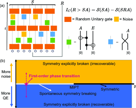
Circuit model. We consider a quantum circuit structure composed of four types of operations, as depicted in Fig. 1(a). Random unitary gates are applied in a brick-wall pattern. Between each pair of unitary layers, each qubit has a probability of being projectively measured along the -axis. The projective measurement can be modeled by first applying a CNOT gate between the system qubit and an environment qubit, followed by another CNOT gate with an ancilla qubit. Tracing out the environment qubit leaves the classical measurement outcome in the ancilla qubit. After the measurement, each qubit has a probability of undergoing a certain noise channel, such as depolarizing, resetting, or dephasing, and a probability of undergoing a QE operation. We denote and . The QE operation involves introducing ancilla qubits and then applying a unitary gate to the system qubit and these ancilla qubits. These ancilla qubits are then isolated, remaining untouched until the end of the circuit. Given that each ancilla qubit is used only once, we assume no noise affects them during the evolution, which is a reasonable assumption considering they can be well-isolated from other qubits, thereby maintaining a coherence time much longer than that of the system qubits. In Refs. [50, 51, 52], the case where noise and QE operations are symmetric was studied. Here, we consider the relative frequency of noise and QE operations, , is no longer constrained to be .
The input state is entangled with a reference system , and the entire quantum circuit can be viewed as a quantum channel from to . Without loss of generality, we consider the scenario where each system qubit is entangled in a Bell pair with a corresponding reference qubit. It is important to note that includes both ancilla qubits from QE operations that store quantum information and those from measurements that only contain classical information. Coherent information, a key quantity for assessing quantum channel capacity, is computed as:
| (1) |
where denoted the entanglement entropy of the subsystem . Our primary focus is to investigate whether a phase transition in occurs as is varied.
Analytical analysis. When random unitary gates are drawn from the Haar measure, the coherent information can be mapped onto the free energy difference of a classical statistical mechanics model under different boundary conditions [55, 56, 57, 58]. Specifically, we have
where
| (3) |
Here, the degrees of freedom of this statistical mechanics model are spins that take values in the permutation group with , and are denoted as . . corresponds to a particular group member in , representing to a particular spin orientation. Thus, can be identified as the bulk partition function, while and correspond to two different boundary conditions. Notice that and represents the top and bottom boundary, respectively.
This statistical mechanics model is a ferromagnetically coupled spin model with random fields oriented in two different directions on a honeycomb lattice [52]. The vertical bond contributes a weight of , where is the Weingarten function, acting as a ferromagnetic coupling that assigns greater weights to configurations where . The non-vertical bonds are determined by the specific choice of QE operations and noise. For instance, if we select and consider depolarizing noise, the bond contributes a weight:
Here, , where is the local Hilbert space dimension and where denotes the number of cycles in permutation . corresponds to the identity element in . Thus, determines the net field direction. For small , the net field aligns with , whereas for large , it aligns with . When combined with the results in Ref. [52], the full phase diagram is depicted in Fig. 1(b). By identifying as the temperature and considering noise and QE operations as two competing external fields, the phase diagram is reminiscent of that of a simple 2D Ising model. Consequently, a first-order phase transition is expected when tuning .
Furthermore, the coherent information can directly detect this first-order phase transition. For small , bulk spins align with , leading to a domain wall at the bottom boundary when calculating , with no additional energy cost in . This results in a positive and is extensive in system size. Conversely, for large , bulk spins align with . In this scenario, a domain wall at the top boundary always exists, while an extra domain wall appears in calculating at the bottom boundary, rendering negative. Since positive indicates that finite amount of quantum information can be successfully transmitted through the channel, which can be recovered via a decoding algorithm, this first-order phase transition corresponds to a transition from a recoverable to an irrecoverable phase.
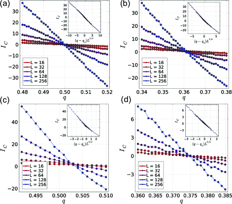
Numerical results. To explicitly demonstrate the existence of the coherent information phase transition, we perform numerical simulations on a large scale. In these simulations, random unitary gates are selected from the Clifford group to enable the use of the stabilizer formalism [59, 60, 61]. We set and specifically consider three types of noise: resetting, depolarizing, and dephasing. Here we set , while results for other parameters can be found in Supplemental Material [62]. We first consider the case with , and the results are presented in Fig. 2(a)-2(c). A distinct recoverable phase, characterized by positive coherent information, is identified. Through data collapse, we determine the critical points and critical exponents to be , and , with , and , respectively. The recoverable phase region is smallest for depolarizing noise and largest for dephasing noise, consistent with the relative strengths of the corresponding random fields [62]. When measurements are incorporated, the phase transition persists, as demonstrated in Fig. 2(d) for depolarizing noise, albeit at a different critical point with . Additional numerical details and results are provided in [62].
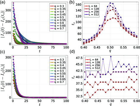
Another interesting phenomenon we observed is critical slowing down [63, 64, 65, 66]. As illustrated in Fig. 3(a), the convergence of the coherent information slows significantly near for resetting noise. By defining the convergence time as the time when first falls below , we plot as a function of for different system sizes in Fig. 3(b). The results indicate that diverges with system size as approaches the critical point, suggesting an infinite convergence time in the thermodynamic limit. In contrast, in the absence of unitary gates, while the coherent information still transitions from positive to negative precisely at (corresponding to the scenario where half of the system qubits are discarded), critical slowing down was not observed, as shown in Fig. 3(c) and 3(d). This observation underscores the indispensability of unitary gates for the manifestation of a phase transition.
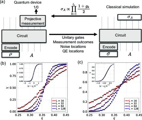
Efficient protocol. Measuring coherent information for a specific circuit and trajectory requires repeated preparation of the same final state. However, in realistic experiments, noise locations are usually uncontrollable, making it difficult to reliably reproduce the same circuit. This issue is compounded by the post-selection problem when measurements are involved, due to Born’s rule [67, 68, 54]. Motivated by previous work on constructing post-selection-free probes that reflect the correlation between a quantum device and classical simulations [69, 53, 70], we propose a resource-efficient protocol to observe the coherent information phase transition. In the quantum device, an initial state is prepared and encoded by the application of random unitary gates alone. This encoded state then undergoes the circuit, with ancillary qubits introduced during the evolution. The unnormalized final state on is denoted as , with , where represents the probability of the particular trajectory . For brevity, we omit the explicit dependence on the circuit realization , which includes choices of random unitary gates and locations of noise, QE operations and measurements. Leveraging the knowledge of the measurement outcomes and the circuit realization, we execute a classical simulation of the same circuit, but with the input state being the encoded state of a distinct state . Assuming the unitary gates are Clifford gates and is a stabilizer state, the classical simulation becomes computationally efficient. We then also obtain , with . It is worth noting that the initial state can be chosen beyond stabilizer states, making the evolution intractable on a classical computer.
The quantity that serves as a proxy for the phase transition is constructed as follows:
| (4) | |||||
Here, represents averaging over different circuit realizations, is the number of measurements with random outcomes during the classical simulation, represents the number of generators for the normalized stabilizer state and are the corresponding generators. The middle term is either or due to the property of stabilizer formalism, while the final term corresponds to the probability of measuring all the generators with outcomes equal to . For each execution of the quantum circuit, we first compute by classical simulation. If the result is , we proceed to perform projective measurements on the ancilla qubits according to the stabilizer generators. If all measurement outcomes are , we denote this as a successful event. The quantity is then estimated as the proportion of successful events among all circuit executions. The whole procedure is outlined in Fig. 4(a). Remarkably, this approach allows us to fully leverage each circuit realization and trajectory, circumventing the need for experimental control over noise locations or post-selection on measurement outcomes.
Physically, this probe reflects the distinguishability of different initial states by leveraging access to both the measurement outcomes and the final state of the ancilla qubits. In the recoverable phase, the initial information is preserved, and we therefore expect , corresponding to perfect distinguishability. Conversely, in the irrecoverable phase, the initial information becomes erased, causing to approach 1. A detailed analytical analysis of this protocol is provided in [62]. To demonstrate the efficacy of this probe, we present numerical results in Fig. 4(b) and Fig. 4(c) for the case of depolarizing noise with and , respectively. The critical points are determined to be and , which are in agreement with the exact phase transition points.
Discussions. The coherent information is related to the single-shot quantum channel capacity by the relation [9, 2]. Here we consider to be a direct product of Bell pairs between and . Through analytical mapping, it is evident that this choice maximizes the coherent information within the recoverable phase, minimizing the free energy . However, in the irrecoverable phase, selecting as a trivial product state would yield zero coherent information, thereby maximizing the coherent information. This results in a phase transition where the single-shot quantum channel capacity shifts from a finite positive value to zero. Furthermore, the true quantum channel capacity , which allows for multiple uses of the channel, becomes additive and equal to only if the channel is degradable [71, 72, 73, 74, 75, 76, 77]. Although measurement and QE operations are all degradable, general noises often lacks this property, making the calculation of more challenging. Thus, it is intriguing to explore whether a phase transition in can be identified within this framework.
A key aspect of the resource-efficient protocol for detecting the coherent information phase transition is the requirement for knowledge of noise locations. In a practical experimental setting, it has been demonstrated that various types of noise can be effectively converted into erasure errors, which can be located by verifying whether the qubit remains in the computational subspace [78, 79, 80, 81, 82, 83, 84, 85, 86]. Upon detection of an erasure error, replacing the qubit with a maximally mixed state corresponds to a depolarizing noise, while replacing it with corresponds to a resetting noise. It is therefore of interest to investigate whether imperfect detection of erasure errors would compromise the protocol’s success. We leave this to future work.
Acknowledgements.
Acknowledgment. We are deeply indebted to Xiao-Liang Qi for many valuable discussions. This work is supported by the National Key Research Program of China under Grant No. 2019YFA0308404, the Natural Science Foundation of China through Grants No. 12350404 and No. 12174066, the Innovation Program for Quantum Science and Technology through Grant No. 2021ZD0302600, the Science and Technology Commission of Shanghai Municipality under Grants No. 23JC1400600 and No. 2019SHZDZX01.References
- Horodecki et al. [2009] R. Horodecki, P. Horodecki, M. Horodecki, and K. Horodecki, Quantum entanglement, Rev. Mod. Phys. 81, 865 (2009).
- Nielsen and Chuang [2010] M. A. Nielsen and I. L. Chuang, Quantum computation and quantum information (Cambridge university press, 2010).
- Carlesso [2024] M. Carlesso, Lecture notes on quantum algorithms in open quantum systems (2024), arXiv:2406.11613 [quant-ph] .
- Koashi and Winter [2004] M. Koashi and A. Winter, Monogamy of quantum entanglement and other correlations, Phys. Rev. A 69, 022309 (2004).
- Schumacher and Nielsen [1996] B. Schumacher and M. A. Nielsen, Quantum data processing and error correction, Phys. Rev. A 54, 2629 (1996).
- Schumacher and Westmoreland [2002] B. Schumacher and M. D. Westmoreland, Approximate quantum error correction, Quantum Information Processing 1, 5 (2002).
- Horodecki et al. [2006] M. Horodecki, J. Oppenheim, and A. Winter, Quantum State Merging and Negative Information, Commun. Math. Phys. 269, 107 (2006).
- Schumacher [1996] B. Schumacher, Sending entanglement through noisy quantum channels, Phys. Rev. A 54, 2614 (1996).
- Wilde [2013] M. M. Wilde, Quantum information theory (Cambridge university press, 2013).
- Gottesman [2009] D. Gottesman, An introduction to quantum error correction and fault-tolerant quantum computation (2009), arXiv:0904.2557 [quant-ph] .
- Dennis et al. [2002] E. Dennis, A. Kitaev, A. Landahl, and J. Preskill, Topological quantum memory, J. Math. Phys. 43, 4452 (2002).
- Wang et al. [2003] C. Wang, J. Harrington, and J. Preskill, Confinement-Higgs transition in a disordered gauge theory and the accuracy threshold for quantum memory, Ann. Phys. 303, 31 (2003).
- Kitaev [1997] A. Yu. Kitaev, Quantum Error Correction with Imperfect Gates, in Quantum Communication, Computing, and Measurement, edited by O. Hirota, A. S. Holevo, and C. M. Caves (Springer US, Boston, MA, 1997) pp. 181–188.
- Terhal [2015] B. M. Terhal, Quantum error correction for quantum memories, Rev. Mod. Phys. 87, 307 (2015).
- Kitaev [2003] A. Y. Kitaev, Fault-tolerant quantum computation by anyons, Ann. Phys. 303, 2 (2003).
- Sekino and Susskind [2008] Y. Sekino and L. Susskind, Fast scramblers, J. High Energy Phys. 2008 (10), 065.
- Mi et al. [2021] X. Mi, P. Roushan, C. Quintana, S. Mandrà, J. Marshall, C. Neill, F. Arute, K. Arya, J. Atalaya, R. Babbush, J. C. Bardin, R. Barends, J. Basso, A. Bengtsson, S. Boixo, A. Bourassa, M. Broughton, B. B. Buckley, D. A. Buell, B. Burkett, N. Bushnell, Z. Chen, B. Chiaro, R. Collins, W. Courtney, S. Demura, A. R. Derk, A. Dunsworth, D. Eppens, C. Erickson, E. Farhi, A. G. Fowler, B. Foxen, C. Gidney, M. Giustina, J. A. Gross, M. P. Harrigan, S. D. Harrington, J. Hilton, A. Ho, S. Hong, T. Huang, W. J. Huggins, L. B. Ioffe, S. V. Isakov, E. Jeffrey, Z. Jiang, C. Jones, D. Kafri, J. Kelly, S. Kim, A. Kitaev, P. V. Klimov, A. N. Korotkov, F. Kostritsa, D. Landhuis, P. Laptev, E. Lucero, O. Martin, J. R. McClean, T. McCourt, M. McEwen, A. Megrant, K. C. Miao, M. Mohseni, S. Montazeri, W. Mruczkiewicz, J. Mutus, O. Naaman, M. Neeley, M. Newman, M. Y. Niu, T. E. O’Brien, A. Opremcak, E. Ostby, B. Pato, A. Petukhov, N. Redd, N. C. Rubin, D. Sank, K. J. Satzinger, V. Shvarts, D. Strain, M. Szalay, M. D. Trevithick, B. Villalonga, T. White, Z. J. Yao, P. Yeh, A. Zalcman, H. Neven, I. Aleiner, K. Kechedzhi, V. Smelyanskiy, and Y. Chen, Information scrambling in quantum circuits, Science 374, 1479 (2021).
- Landsman et al. [2019] K. A. Landsman, C. Figgatt, T. Schuster, N. M. Linke, B. Yoshida, N. Y. Yao, and C. Monroe, Verified quantum information scrambling, Nature 567, 61 (2019).
- Li et al. [2019] Y. Li, X. Chen, and M. P. A. Fisher, Measurement-driven entanglement transition in hybrid quantum circuits, Phys. Rev. B 100, 134306 (2019).
- Chan et al. [2019] A. Chan, R. M. Nandkishore, M. Pretko, and G. Smith, Unitary-projective entanglement dynamics, Phys. Rev. B 99, 224307 (2019).
- Bao et al. [2024] Y. Bao, M. Block, and E. Altman, Finite-Time Teleportation Phase Transition in Random Quantum Circuits, Phys. Rev. Lett. 132, 030401 (2024).
- Lee et al. [2022] J. Y. Lee, W. Ji, Z. Bi, and M. P. A. Fisher, Decoding measurement-prepared quantum phases and transitions: from ising model to gauge theory, and beyond (2022), arXiv:2208.11699 [cond-mat.str-el] .
- Li et al. [2023a] Y. Li, S. Vijay, and M. P. Fisher, Entanglement domain walls in monitored quantum circuits and the directed polymer in a random environment, PRX Quantum 4, 010331 (2023a).
- Nahum and Skinner [2020] A. Nahum and B. Skinner, Entanglement and dynamics of diffusion-annihilation processes with majorana defects, Phys. Rev. Research 2, 023288 (2020).
- Nahum et al. [2018] A. Nahum, S. Vijay, and J. Haah, Operator spreading in random unitary circuits, Phys. Rev. X 8, 021014 (2018).
- Nahum et al. [2017] A. Nahum, J. Ruhman, S. Vijay, and J. Haah, Quantum entanglement growth under random unitary dynamics, Phys. Rev. X 7, 031016 (2017).
- Sharma et al. [2022] S. Sharma, X. Turkeshi, R. Fazio, and M. Dalmonte, Measurement-induced criticality in extended and long-range unitary circuits, SciPost Phys. Core 5, 023 (2022).
- Sang et al. [2021] S. Sang, Y. Li, T. Zhou, X. Chen, T. H. Hsieh, and M. P. Fisher, Entanglement negativity at measurement-induced criticality, PRX Quantum 2, 030313 (2021).
- Skinner et al. [2019] B. Skinner, J. Ruhman, and A. Nahum, Measurement-induced phase transitions in the dynamics of entanglement, Phys. Rev. X 9, 031009 (2019).
- Szyniszewski et al. [2019] M. Szyniszewski, A. Romito, and H. Schomerus, Entanglement transition from variable-strength weak measurements, Phys. Rev. B 100, 064204 (2019).
- Vasseur et al. [2019] R. Vasseur, A. C. Potter, Y.-Z. You, and A. W. W. Ludwig, Entanglement transitions from holographic random tensor networks, Phys. Rev. B 100, 134203 (2019).
- Zabalo et al. [2020] A. Zabalo, M. J. Gullans, J. H. Wilson, S. Gopalakrishnan, D. A. Huse, and J. H. Pixley, Critical properties of the measurement-induced transition in random quantum circuits, Phys. Rev. B 101, 060301 (2020).
- Alberton et al. [2021] O. Alberton, M. Buchhold, and S. Diehl, Entanglement Transition in a Monitored Free-Fermion Chain: From Extended Criticality to Area Law, Phys. Rev. Lett. 126, 170602 (2021).
- Fidkowski et al. [2021] L. Fidkowski, J. Haah, and M. B. Hastings, How dynamical quantum memories forget, Quantum 5, 382 (2021).
- Fisher et al. [2023] M. P. A. Fisher, V. Khemani, A. Nahum, and S. Vijay, Random Quantum Circuits, Annu. Rev. Condens. Matter Phys. 14, 335 (2023).
- Poboiko et al. [2024] I. Poboiko, I. V. Gornyi, and A. D. Mirlin, Measurement-induced phase transition for free fermions above one dimension, Phys. Rev. Lett. 132, 110403 (2024).
- Yu and Qi [2022] X. Yu and X.-L. Qi, Measurement-induced entanglement phase transition in random bilocal circuits (2022), arXiv:2201.12704 [quant-ph] .
- Choi et al. [2020] S. Choi, Y. Bao, X.-L. Qi, and E. Altman, Quantum Error Correction in Scrambling Dynamics and Measurement-Induced Phase Transition, Phys. Rev. Lett. 125, 030505 (2020).
- Gullans and Huse [2020] M. J. Gullans and D. A. Huse, Dynamical purification phase transition induced by quantum measurements, Phys. Rev. X 10, 041020 (2020).
- Dias et al. [2023] B. C. Dias, D. Perković, M. Haque, P. Ribeiro, and P. A. McClarty, Quantum noise as a symmetry-breaking field, Phys. Rev. B 108, L060302 (2023).
- Liu et al. [2023] S. Liu, M.-R. Li, S.-X. Zhang, S.-K. Jian, and H. Yao, Universal KPZ scaling in noisy hybrid quantum circuits, Phys. Rev. B 107, L201113 (2023).
- Liu et al. [2024a] S. Liu, M.-R. Li, S.-X. Zhang, and S.-K. Jian, Entanglement structure and information protection in noisy hybrid quantum circuits, Phys. Rev. Lett. 132, 240402 (2024a).
- Liu et al. [2024b] S. Liu, M.-R. Li, S.-X. Zhang, S.-K. Jian, and H. Yao, Noise-induced phase transitions in hybrid quantum circuits (2024b), arXiv:2401.16631 [quant-ph] .
- Weinstein et al. [2022] Z. Weinstein, Y. Bao, and E. Altman, Measurement-Induced Power-Law Negativity in an Open Monitored Quantum Circuit, Phys. Rev. Lett. 129, 080501 (2022).
- Haas et al. [2024] L. Haas, C. Carisch, and O. Zilberberg, Scrambling-induced entanglement suppression in noisy quantum circuits (2024), arXiv:2408.02810 [quant-ph] .
- Braun et al. [2018] D. Braun, G. Adesso, F. Benatti, R. Floreanini, U. Marzolino, M. W. Mitchell, and S. Pirandola, Quantum-enhanced measurements without entanglement, Rev. Mod. Phys. 90, 035006 (2018).
- Aharonov et al. [2022] D. Aharonov, J. Cotler, and X.-L. Qi, Quantum algorithmic measurement, Nature Commun. 13, 887 (2022).
- Huang et al. [2021] H.-Y. Huang, R. Kueng, and J. Preskill, Information-Theoretic Bounds on Quantum Advantage in Machine Learning, Phys. Rev. Lett. 126, 190505 (2021).
- Zhao et al. [2017] J. Zhao, J. Dias, J. Y. Haw, M. Bradshaw, R. Blandino, T. Symul, T. C. Ralph, S. M. Assad, and P. K. Lam, Quantum enhancement of signal-to-noise ratio with a heralded linear amplifier, Optica 4, 1421 (2017).
- Kelly and Marino [2024a] S. P. Kelly and J. Marino, Entanglement transitions in quantum-enhanced experiments (2024a), arXiv:2310.03061 [quant-ph] .
- Kelly and Marino [2024b] S. P. Kelly and J. Marino, Generalizing measurement-induced phase transitions to information exchange symmetry breaking (2024b), arXiv:2402.13271 [quant-ph] .
- Qian and Wang [2024a] D. Qian and J. Wang, Protect measurement-induced phase transition from noise (2024a), arXiv:2406.14109 [quant-ph] .
- Li et al. [2023b] Y. Li, Y. Zou, P. Glorioso, E. Altman, and M. P. A. Fisher, Cross entropy benchmark for measurement-induced phase transitions, Phys. Rev. Lett. 130, 220404 (2023b).
- Friedman et al. [2023] A. J. Friedman, O. Hart, and R. Nandkishore, Measurement-Induced Phases of Matter Require Feedback, PRX Quantum 4, 040309 (2023).
- Bao et al. [2020] Y. Bao, S. Choi, and E. Altman, Theory of the phase transition in random unitary circuits with measurements, Phys. Rev. B 101, 104301 (2020).
- Jian et al. [2020] C.-M. Jian, Y.-Z. You, R. Vasseur, and A. W. W. Ludwig, Measurement-induced criticality in random quantum circuits, Phys. Rev. B 101, 104302 (2020).
- Zhou and Nahum [2019] T. Zhou and A. Nahum, Emergent statistical mechanics of entanglement in random unitary circuits, Phys. Rev. B 99, 174205 (2019).
- Li et al. [2021] Y. Li, X. Chen, A. W. W. Ludwig, and M. P. A. Fisher, Conformal invariance and quantum nonlocality in critical hybrid circuits, Phys. Rev. B 104, 104305 (2021).
- Aaronson and Gottesman [2004] S. Aaronson and D. Gottesman, Improved simulation of stabilizer circuits, Phys. Rev. A 70, 052328 (2004).
- Gottesman [1998] D. Gottesman, The heisenberg representation of quantum computers (1998), arXiv:quant-ph/9807006 [quant-ph] .
- Gottesman [1997] D. Gottesman, Stabilizer codes and quantum error correction (1997), arXiv:quant-ph/9705052 [quant-ph] .
- [62] See Supplemental Material for technical details.
- Marconi et al. [2024] M. Marconi, K. Alfaro-Bittner, L. Sarrazin, M. Giudici, and J. R. Tredicce, Critical slowing down in a real physical system (2024), arXiv:2403.17973 [cond-mat.stat-mech] .
- Scheffer et al. [2009] M. Scheffer, J. Bascompte, W. A. Brock, V. Brovkin, S. R. Carpenter, V. Dakos, H. Held, E. H. Van Nes, M. Rietkerk, and G. Sugihara, Early-warning signals for critical transitions, Nature 461, 53 (2009).
- Van Hove [1954] L. Van Hove, Time-Dependent Correlations between Spins and Neutron Scattering in Ferromagnetic Crystals, Phys. Rev. 95, 1374 (1954).
- Li et al. [2022] X. Li, X. Luo, S. Wang, K. Xie, X.-P. Liu, H. Hu, Y.-A. Chen, X.-C. Yao, and J.-W. Pan, Second sound attenuation near quantum criticality, Science 375, 528 (2022).
- Qian and Wang [2024b] D. Qian and J. Wang, Steering-induced phase transition in measurement-only quantum circuits, Phys. Rev. B 109, 024301 (2024b).
- Paviglianiti et al. [2024] A. Paviglianiti, G. D. Fresco, A. Silva, B. Spagnolo, D. Valenti, and A. Carollo, Breakdown of measurement-induced phase transitions under information loss (2024), arXiv:2407.13837 [quant-ph] .
- Garratt and Altman [2024] S. J. Garratt and E. Altman, Probing postmeasurement entanglement without postselection, PRX Quantum 5, 030311 (2024).
- McGinley [2024] M. McGinley, Postselection-Free Learning of Measurement-Induced Quantum Dynamics, PRX Quantum 5, 020347 (2024).
- Holevo [1998] A. S. Holevo, The capacity of the quantum channel with general signal states, IEEE Trans. Inf. Theory 44, 269 (1998).
- Devetak and Shor [2005] I. Devetak and P. W. Shor, The Capacity of a Quantum Channel for Simultaneous Transmission of Classical and Quantum Information, Commun. Math. Phys. 256, 287 (2005).
- Hastings [2009] M. B. Hastings, Superadditivity of communication capacity using entangled inputs, Nature Phys. 5, 255 (2009).
- Devetak [2005] I. Devetak, The Private Classical Capacity and Quantum Capacity of a Quantum Channel, IEEE Trans. Inf. Theory 51, 44 (2005).
- Lloyd [1997] S. Lloyd, Capacity of the noisy quantum channel, Phys. Rev. A 55, 1613 (1997).
- DiVincenzo et al. [1998] D. P. DiVincenzo, P. W. Shor, and J. A. Smolin, Quantum-channel capacity of very noisy channels, Phys. Rev. A 57, 830 (1998).
- Barnum et al. [2000] H. Barnum, E. Knill, and M. Nielsen, On quantum fidelities and channel capacities, IEEE Trans. Inf. Theory 46, 1317 (2000).
- Delfosse and Zémor [2020] N. Delfosse and G. Zémor, Linear-time maximum likelihood decoding of surface codes over the quantum erasure channel, Phys. Rev. Research 2, 033042 (2020).
- Solanki and Sarvepalli [2023] H. M. Solanki and P. K. Sarvepalli, Decoding topological subsystem color codes over the erasure channel using gauge fixing, IEEE Trans. Commun. 71, 4181 (2023).
- Grassl et al. [1997] M. Grassl, T. Beth, and T. Pellizzari, Codes for the Quantum Erasure Channel, Phys. Rev. A 56, 33 (1997).
- Bennett et al. [1997] C. H. Bennett, D. P. DiVincenzo, and J. A. Smolin, Capacities of Quantum Erasure Channels, Phys. Rev. Lett. 78, 3217 (1997).
- Chang et al. [2024] K. Chang, S. Singh, J. Claes, K. Sahay, J. Teoh, and S. Puri, Surface code with imperfect erasure checks (2024), arXiv:2408.00842 [quant-ph] .
- Kang et al. [2023] M. Kang, W. C. Campbell, and K. R. Brown, Quantum Error Correction with Metastable States of Trapped Ions Using Erasure Conversion, PRX Quantum 4, 020358 (2023).
- Wu et al. [2022] Y. Wu, S. Kolkowitz, S. Puri, and J. D. Thompson, Erasure conversion for fault-tolerant quantum computing in alkaline earth Rydberg atom arrays, Nature Commun. 13, 4657 (2022).
- Kubica et al. [2023] A. Kubica, A. Haim, Y. Vaknin, H. Levine, F. Brandão, and A. Retzker, Erasure Qubits: Overcoming the T 1 Limit in Superconducting Circuits, Phys. Rev. X 13, 041022 (2023).
- Gu et al. [2024] S. Gu, Y. Vaknin, A. Retzker, and A. Kubica, Optimizing quantum error correction protocols with erasure qubits (2024), arXiv:2408.00829 [quant-ph] .