Low Saturation Confidence Distribution-based Test-Time Adaptation for Cross-Domain Remote Sensing Image Classification

Abstract

Although the Unsupervised Domain Adaptation (UDA) method has greatly improved the effect of remote sensing image classification tasks, most of them are still limited by access to the source domain (SD) data. Designs such as Source-free Domain Adaptation (SFDA) solve the challenge of a lack of SD data, however, they still rely on a large amount of target domain data and thus cannot achieve fast adaptations, which seriously hinders their further application in broader scenarios. The real-world applications of cross-domain remote sensing image classification require a balance of speed and accuracy at the same time. Therefore, we propose a novel and comprehensive test time adaptation (TTA) method – Low Saturation Confidence Distribution Test Time Adaptation (LSCD-TTA), which is the first attempt to solve such scenarios through the idea of TTA. LSCD-TTA specifically considers the distribution characteristics of remote sensing images, including three main parts that concentrate on different optimization directions: First, low saturation distribution (LSD) considers the dominance of low-confidence samples during the later TTA stage. Second, weak-category cross-entropy (WCCE) increases the weight on categories that are more difficult to classify with less prior knowledge. Finally, diverse categories confidence (DIV) comprehensively considers the category diversity to alleviate the deviation of the sample distribution. Through a weighting of the abovementioned three modules, the model can widely, quickly and accurately adapt to the target domain without much prior target distributions, repeated data access, and manual annotation. We evaluate LSCD-TTA on three remote sensing image datasets. The experimental results show that LSCD-TTA achieves a significant gain of 4.96$\%$-10.51$\%$ with Resnet-50 and 5.33$\%$-12.49$\%$ with Resnet-101 in average accuracy compared to other state-of-the-art DA and TTA methods, and also achieves quite competitive performance in robust evaluation metrics such as variance.

I Introduction

Due to their ability to efficiently extract feature information from remote sensing data and excel in several aspects, deep learning approaches are being widely used in remote sensing image classification tasks [1, 2, 3, 4]. Nevertheless, the inherent variability and diversity in remote sensing data distributions impose distinct and complex demands on cross-domain remote sensing models. Common approaches to address such dilemma involve either merging labeled target domain (TD) data with source domain (SD) data for retraining or fine-tuning pre-trained models using specific target domain datasets. However, regardless of the approach taken, the model’s effectiveness is largely contingent on the quality of labeled data. Furthermore, the diversity in land categories, high information density, and variable meteorological conditions in remote sensing images further complicates accurate annotation. Consequently, label-dependent methods are often impractical due to the inefficiency and high cost of obtaining sufficient annotated data.

As shown in Fig. 1, Unsupervised Domain Adaptation (UDA) [5] proposes a new idea to solve the abovementioned challenge. Common UDA strategies enhance the model’s ability to generalize across domains without labeled target data, such as feature mapping and alignment methods [6, 7], adversarial training methods [8, 9] and pseudo-labeling methods [10, 11]. These abovementioned achievements demonstrate the notable performance of UDA in practical application scenarios in the remote sensing community. However, these UDA methods still require the incorporation of both source and target domain data for retraining to update the model. The growing input dimensionality and model complexity significantly increase computational costs for processing new data. Moreover, in many remote sensing scenarios where data privacy is a concern (e.g. military monitoring, resource detection [12]), the model builder usually does not have access to the SD data. Such scenarios also pose a practical challenge to UDA models. To address this challenge, Source-free Domain Adaptation (SFDA) [13] has been introduced as a solution, allowing the adaptation of pre-trained SD models to arbitrary invisible target domains without requiring access to the source data.

Advanced SFDA methods leverage the pre-trained source model to generate pseudo-labels for self-supervised training [14], engage in contrastive learning tasks [15], or employ adversarial training strategies [16] to avoid the redundant retraining that involves both source and TD data, as well as to eliminate the need for accessing SD data. However, SFDA methods typically require considerable TD data for effective adaptation. Therefore, multiple iterations are required to progressively align with the TD distribution. In remote sensing scenarios, the high information density, category diversity, and meteorological uncertainties make the limitation of SFDA particularly pronounced. For example, UAV-based disaster monitoring [17] require models to quickly detect geo-climatic situations and provide accurate trend analysis and early warnings across diverse regions. Similarly, in fast-paced military operations, real-time monitoring of enemy positions and equipment demands rapid model adaptation. While these scenarios may operate under source-free conditions, the extensive target data and iterative cycles required in SFDA often hinder models from adapting swiftly to real-time changes across broader areas. Consequently, traditional DA models struggle to surpass the limitations of offline learning when faced with urgent real-time demands. Given the timeliness and privacy concerns, online learning has gained significant attention to better adapt to real-time and dynamic updating for adaptation models while safeguarding data privacy.

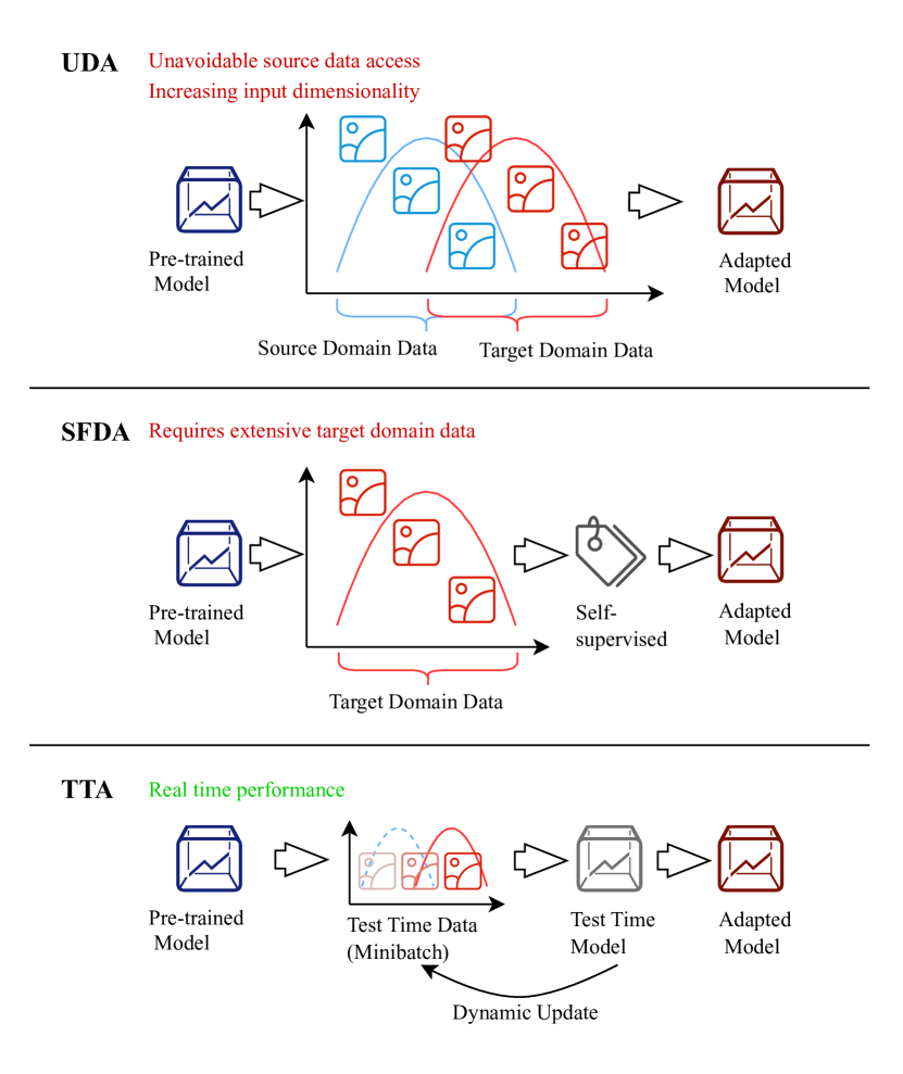
Figure 1: Comparisons of different domain adaptation methods for remote sensing image classification.

Test Time Adaptation (TTA) [18], as a novel extension method of online learning, is a pivotal component that empowers models to dynamically adapt and update to new test data in real-time applications. In the process of TTA, we continue to accept small batches of TD data and perform unsupervised fine-tuning of the SD pre-trained model. Unlike traditional fine-tuning, TTA dynamically updates the model based on feedback from new mini test data, occurring during the testing phase rather than training. Such an approach minimizes training interference while enhancing model stability and performance. When new test samples arrive, the model adapts to the current data distribution and features without needing repeated access to SD data, enabling efficient updates and generalization while maintaining data privacy. So far, classic TTA approaches [18, 19] can be better adapted to the needs of changing data and dynamic environments. However, most of these advanced TTA methods have only validated their effectiveness on artificially corrupted datasets (e.g., CIFAR10-C [20]), which is different from real-world scenarios with multiple cross-domain styles in DA tasks, especially in high information density, changing meteorological environments, large-scale remote sensing scenarios. Although TTA can rapidly adjust and refine the model on continuous mini-batch TD data in a manner similar to "unsupervised fine-tuning", its direct application in cross-domain remote sensing image classification tasks still needs further optimization.

In this paper, we focus on real-time remote sensing scene classification, without repeated access to SD data or labeled annotations. We propose a TTA method based on the characteristics of remote sensing images, to rapidly and accurately adapt SD models to changing areas. In summary, the contributions of this paper can be highlighted in the following three aspects.

1. We propose a comprehensive TTA method LSCD-TTA for quickly and accurately cross-domain remote sensing image classification. To the best of our knowledge, LSCD-TTA the first attempt to integrate TTA with cross-domain classification tasks within the remote sensing community.

2. LSCD-TTA introduces three modules (i.e., LSD, WCCE, DIV) to enhance low-confidence sample performance, improve weak category classification, and mitigate cross-category distribution bias. Such a design comprehensively considers the specific characteristics of remote sensing images, which addresses the challenges when directly applied classic-TTA to remote sensing image data.

3. We conduct comprehensive experiements and analysis to exhibit the superiority of LSCD-TTA on three open-source remote sensing datasets where LSCD-TTA outperforms state-of-the-art DA and TTA methods remarkably of 4.96$\%$-10.51$\%$ with Resnet-50 and 5.33$\%$-12.49$\%$ with Resnet-101 in average accuracy, and also achieves a quite competitive performance in robustness.

The subsequent sections are organized as follows: We first summarize the relevant research in Section II. Sequentially, we elaborate our proposed LSCD-TTA in Section III, and give a brief introduction of datasets in Section IV. Section V presents the configuration, corresponding results and validation of DA experiments on these datasets. Finally, we discuss and summarize our work in Section VI and Section VII.

II Related works

II-A UDA and SFDA

By adopting simple yet efficient designs such as adversarial learning [21, 9], feature alignment [22, 23] and pseudo-labeling [24, 25], UDA [5] successfully tackles the challenge of label unavailability by employing innovative learning strategies that require no labeled data from the target domain. For example, Lee et al. [21] enhance UDA by employing adversarial dropout techniques to develop highly discriminative feature representations that support robust domain adaptation across different tasks. Zhang et al. [22] introduced Spectral UDA to enhance and align domain-invariant features and suppress domain-variant ones for improved UDA across various visual tasks. Wang et al. [24] introduced a novel selective pseudo-labeling strategy, adopting unsupervised deep feature space clustering analysis to facilitate accurate pseudo-labeling. However, the implementation of existing UDA methods inevitably requires access to SD data and involves retraining with source and target domain data. Such a demand leads to unavoidable access to source data and a continual increase in input dimensions. In broader real-world scenarios where source data is inaccessible, these methods still exhibit significant limitations.

Following the successes of UDA in tackling challenges within cross-scene remote sensing image classification, the concept of SFDA [13] was introduced to address scenarios where source domain data is inaccessible. SFDA leverages pre-trained source models to adapt directly to target domains without source data access, typically using pseudo-labels [26, 27] and self-training strategies [28, 29]. Tang et al. [30] developed a novel method for SFDA using a frozen multimodal foundation model to improve adaptation performance. Mitsuzumi et al. [31] offered a theoretical framework for SFDA, resulting in an improved method with auto-adjusting diversity and augmentation training. While SFDA is renowned for its exceptional adaptability and flexibility across various tasks, it requires extensive TD data to perform effectively. It can be a limitation in real-time applications where rapid response is crucial for decision-making. Such a demand highlights its challenges in broader and more immediate application contexts.

II-B Test Time Adaptation

Different from classic DA approaches, Test Time Adaptation (TTA) [18] is independent of retraining with source domain datasets or substantial target data, but to adjust and update trained classifiers using only mini-batch online unlabeled target data. Owing to its retraining-free and real-time responsiveness characteristics, several TTA methods have been proposed to address the DA problems and applied in the computer vision community, particularly in rapidly changing environments. Existing advanced TTA methods concentrate mostly on self-supervised learning methods [32, 33, 34], feature alignment ideas [35, 36, 37], optimization-based [38, 39, 40] and regularization-based [41, 19] model reconstruction strategy. For example, Ma et al. [34] construct a graph structure to correct the enhanced pseudo-labels based on the similarity of the latent features to achieved a robust TTA process. Wang et al. [35] calculated the output probability of $\mathcal{K}$ nearest-neighbor features to reduce the effect of domain bias. Boudiaf et al. [19] used an efficient concave procedure and Laplace optimization to adjust the maximum likelihood estimation objective to address the uncertainty in the testing process.

Despite the success of advanced TTA methods in classic cross-domain classification tasks, they often depend on well-structured data distributions for accurate high-confidence predictions. In real-world scenarios that involve much more changes, TTA still faced a severe challenge to domains including multiple categories and blurred boundary distributions on information-rich data, especially when the DA model only received limited prior knowledge from the source domain. However, in much more dynamic real-world scenarios, TTA still faces significant challenges with domains containing multiple categories and blurred boundaries, particularly when the DA model has limited prior knowledge from the source domain and adapts to an information-rich domain. Accordingly, there remains a pressing need for practical TTA methods tailored to complex cross-domain image classification tasks.

II-C Domain Adaptation in Remote Sensing

Domain adaptation (DA) has emerged as a vital technique in remote sensing, tackling issues such as limited labeled data and variations from different sensors and environmental conditions that impair model generalization across diverse scenarios. Researchers have already achieved a series of successes in remote sensing image tasks with DA methods, ranging from classification [8, 42], semantic segmentation [43, 44], object detection [45, 46, 47], and regression tasks [48, 49], etc. For the issue of image classification in the field of remote sensing, UDA [6, 9] and SFDA [50, 51] have shown significant progress in the field of cross-domain remote sensing image classification. However, despite these advancements, both UDA and SFDA face significant challenges in real-time adaptation of cross-region scene classification, where the complexity and speed demands exceed the capabilities of traditional DA methods.

Although advanced Test-Time Adaptation (TTA) methods reach a balance on real-time adaptation and accurate classification in simple classification tasks, given the inherent data diversity and changing conditions of remote sensing image data, directly applying advanced TTA methods can be particularly challenging. To date, as far as we know, there has been no work that introduces TTA into remote sensing image classification tasks, particularly for scenarios requiring high-resolution and real-time image classification. TTA for remote sensing presents a promising avenue for addressing these abovementioned challenges by adapting models on the fly to new, unseen data without requiring access to the source domain. Our work aims to bridge the gap by proposing a novel TTA method tailored to the demands of cross-domain large-scale remote sensing image classification.

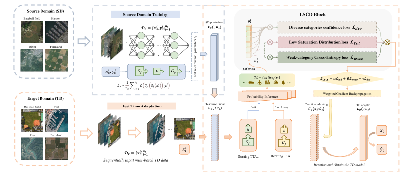
Figure 2: The main structure of our proposed LSCD-TTA involves two main parts: i.e., model training process with source domain data and test time adaptation process with LSCD. As shown in the figure, in the context of data from the SD and the TD sharing the same categories but differing in distribution, we first train the model $F_{\theta}(\cdot;\theta_{s})$ based on the SD knowledge. Sequentially, LSCD-TTA extracts the features of the mini-batch unsupervised TD images within the continuous input and calculates the probability distribution using the classification model $G_{\theta}(\cdot;\theta_{s})$, which is initialized by $F_{\theta}(\cdot;\theta_{s})$. During the following TTA process, with softmax logits, our proposed LSCD block considers the overall distribution of the domain (i.e. $\mathcal{L}_{div}$) and especially emphasizes low-saturation or week-probability samples that are difficult to distinguish (i.e. $\mathcal{L}_{lsd}$ and $\mathcal{L}_{wcce}$), so as to align the SD and TD in real time. By updating the test time model $G_{\theta}^{\prime}(x_{t}^{i};\theta_{t}^{\prime})$ through unsupervised TD data by weighted gradient backpropagation, LSCD-TTA allows the SD pre-trained model to be finetuned unsupervised online, resulting in the high accuracy and robustness of the final TD classification model $G_{\theta}(\cdot;\theta_{t})$.

III Methodology

In this paper, we propose a novel TTA method, termed Low Saturation Confidence Distribution Test Time Adaptation (LSCD-TTA), which is designed to address the challenges encountered by traditional methods in large-scale cross-scene remote sensing image classification tasks. In addition to comprehensively analyzing the uncertainty and diversity distribution in the target domain, we design three novel losses for feature-aligned that consider low-saturation, weak-probability, and overall diversity respectively. As a result, LSCD-TTA significantly enhances the model’s generalization capability to the target domain through the integration of the abovementioned designs. Beyond addressing the complexity of cross-scene remote sensing image classification, LSCD-TTA also offers a novel perspective and solution for the broader application of TTA techniques within the remote sensing community. We generally address the above adaptation task during the cross-scenario test-time process in three steps (See Fig. 2).

1. Train with a unified backbone (such as ResNet) only with the source domain (SD) data, so as to learn the SD knowledge and generate the pre-trained SD model.

2. Transfer the pre-trained SD model (including SD distribution, SD assumptions, etc.) to the target domain (TD) without accessing the source data.

3. Design a better network architecture for the TTA process on the TD, including different ways for feature alignment, multiple designs of the loss for different tasks, etc.

III-A Problem preliminaries

Suppose that there are $n_{s}$ labeled samples $\{x_{s}^{i},y_{s}^{i}\}_{i=1}^{n_{s}}$ in the SD $\mathcal{D}_{s}$, where $x_{s}^{i},y_{s}^{i}$ represent the training data and the corresponding hard categorization labels of the source domain $\mathcal{D}_{s}$, respectively. Similarly, we assume that there are $n_{t}$ unlabeled sample data $\{x_{t}^{i}\}_{i=1}^{n_{t}}$ in the TD $\mathcal{D}_{t}$, where $x_{t}^{i}\in\mathcal{X}_{t}$.

Significant domain gaps are prevalent in the complex field of remote sensing, where information density is high and meteorological conditions are highly variable. Such complexity poses a formidable challenge for cross-scene classification tasks in the remote sensing field, particularly when confronted with non-negligible domain shifts on a large scale. In the SD model’s training process, we train the feature generator $G_{f}$ to obtain discriminative features of the SD and the label classifier $G_{y}$ to classify the samples into different classes. Throughout the training process, the main focus of training is to minimize the loss between the data labels from the source domain and the predicted labels, that is, optimizing the parameters of $G_{f}$ and $G_{y}$ to reduce the classification loss $\mathcal{L}_{s}$ in the source domain:

$$\mathcal{L}_{s}=\frac{1}{n_{s}}\sum_{i=1}^{n_{s}}\mathcal{L}(G_{y}(G_{f}(x_{s}^{i})),y_{s}^{i})$$ (1)

where $x_{i}^{s}$ and $y_{i}^{s}$ are the samples and labels of the SD respectively, and $\mathcal{L}$ is the classification loss function (e.g., cross-entropy loss) used in the SD training. In the training stage of the SD, the model is trained using SD knowledge parameterized via $\theta\in\Theta$ to derive the SD model $F_{\theta}(\cdot|\theta):\mathcal{X}\to\mathcal{Y}$. Sequentially, we expect the DA model to correctly predict the labels of batches $\{y_{t}^{i}\}_{i=1}^{n_{t}}$ by adapting the training model’s parameter $\theta$ to test distributions with only unlabeled data, where $y_{t}^{i}\in{\mathcal{Y}}_{t}$. Equivalently, we would like the model to generate a categorical mapping relation $f_{t}:\mathcal{X}_{t}\to\mathcal{Y}_{t}$ for the target domain while accepting only unlabeled test data $\{x_{t}^{i}\}_{i=1}^{n_{t}}$ and the SD categorical mapping relation $f_{s}:\mathcal{X}_{s}\to\mathcal{Y}_{s}$.

In short, TTA methods accomplish such an idea in two main steps, which is also shown in Fig. 2:

1. A new network $G_{\mathrm{\theta}}$ is initially generated based on the source domain model $F_{\theta}$, where $\mathrm{\theta}$ denotes the parameters that need to be adapted in the TTA process.

2. In TTA process, an unsupervised loss function $\mathcal{L}$ is used to adapt the parameters $\mathrm{\theta}$ of $G_{\mathrm{\theta}}$ based on the input unlabeled data $\{x_{t}^{i}\}_{i=1}^{n_{t}}$ gain from the target domain.

In this paper, we jointly adopt three novel and effective loss function modules $\mathcal{L}_{\mathrm{wcce}}$, $\mathcal{L}_{\mathrm{div}}$, and $\mathcal{L}_{\mathrm{lsd}}$ for model’s self-supervise adaptation process. The performance of the model under different domains or distributions can be improved tremendously by combining our proposed loss functions.

III-B Parameter iteration

Our approach iterates over the optimization transformation parameters $\gamma,\beta$ in backpropagation by estimating the normalized statistics $\mu,\sigma$ of the test data during the testing process. Such an idea allows the parameters of the model to be updated by re-estimating the normalized statistics from the constant input of TD data without repeated access to the SD data:

$$\mu_{t}=\frac{1}{n_{t}}\sum_{i=1}^{n_{t}}x_{t}^{i}$$ (2)

$$\sigma_{t}^{2}=\frac{1}{n_{t}}\sum_{i=1}^{n_{t}}(x_{t}^{i}-\mu_{\mathrm{t}})^{2}$$

Subsequently, for a given input batch $x_{t}$, a normalization operation is performed on the recomputed statistics:

$$\hat{x_{t}}=\frac{x_{t}-\mu_{t}}{\sqrt{\sigma_{t}^{2}+\epsilon}}$$ (3)

In the optimization transformation process of the backpropagation stage, the transformation parameters include the scaling parameter $\gamma$ and the bias parameter $\beta$ of the Batch Normalization (BN) layer. For each input $x_{t}$ in the target domain, the output of the BN layer can be denoted as:

$$y=\gamma\hat{x}+\beta$$ (4)

In general, one can compute the gradient of these parameters $\frac{\partial\mathcal{L}}{\partial\gamma},\frac{\partial\mathcal{L}}{\partial\beta}$ by means of the loss function $\mathcal{L}$ at the time of testing process, and subsequently back-propagate the gradient to perform the optimization of the transformed parameters:

$$\gamma=\gamma+\frac{\partial\mathcal{L}}{\partial\gamma}$$ (5)

$$\beta=\beta+\frac{\partial\mathcal{L}}{\partial\beta}$$

  Input: Source domain pre-trained model, target domain data

  Output: Fine-tune model

1  Adaptation: Performs online updating, i.e., fine-tuning the model using the target domain data without supervision.

2

  for each mini-batch target domain data $\mathbf{x_{t}}$ do

3     1: Calculate the batch mean and variance:

4 $\mu_{t}=\frac{1}{n_{t}}\sum_{i=1}^{n_{t}}x_{t}^{i},\quad\sigma_{t}^{2}=\frac{1}{n_{t}}\sum_{i=1}^{n_{t}}(x_{t}^{i}-\mu_{t})^{2}$

5     2: Normalize the data: $\hat{x_{t}}=\frac{x_{t}-\mu_{t}}{\sqrt{\sigma_{t}^{2}+\epsilon}}$

6     3: Zoom and pan through the BN layer:

7 $y=\gamma\hat{x_{t}}+\beta$

8     4: Denote the distribution $p$ via the predicted output $y$

9

10     5: Calculate the loss via $\mathcal{L}$ according to Equation 13.

11     6: Backpropagation to compute gradients: $\frac{\partial\mathcal{L}}{\partial\gamma},\frac{\partial\mathcal{L}}{\partial\beta}$

12     7: Update the scaling and bias parameters with SGD:

 $\gamma=\gamma-\eta\frac{\partial\mathcal{L}}{\partial\gamma},\quad\beta=\beta-\eta\frac{\partial\mathcal{L}}{\partial\beta}$

  end for

Algorithm 1 LSCD Test time adaptation

As shown in algorithm 1, the target domain data’s normalized statistics and transformation parameters are updated at each step of the adaptation iteration. During the forward pass, the normalized statistics are estimated layer by layer. Even more noteworthy, as mentioned in Section I, TTA is built on the online learning framework, and the iteration continues as long as the data in the target domain is open and continuous to the model. In other words, the model can continue the TTA process with multiple rounds of updates for continuous updating.

III-C Weak-category Cross-Entropy loss $\mathcal{L}_{\mathrm{wcce}}$

During the TTA process, by inputting each batch of unlabeled target domain data $x_{t}$ into the backbone, the numerical distribution computed from $x_{t}$ can be denoted as $o_{\mathcal{D}_{t}}(y_{t})$. It is naturally expected that the empirical distribution of $G_{\mathrm{\theta}}$ in subsequent updates with $x_{t}$ to match the distribution of the target domain as closely as possible.

In classical DA, cross-entropy loss is often used as a measure of uncertainty in the probability distribution of the TD. Assume that $\hat{p}=G_{\theta}(x)$ is the probability distribution predicted by the model and normalized by softmax transformation, i.e., $\hat{p}=$softmax$(o_{\mathcal{D}_{t}}(y_{t}))$. For more general scenarios, more general distributional probabilities can be represented by $\hat{p}^{g}$, therefore the cross-entropy loss function can be written in a more generally generalizable form:

$$\hat{p}=softmax(o_{\mathcal{D}_{t}}(y_{t}))=\frac{\exp(y_{c})}{\sum_{i=1}^{C}\exp(y_{i})}$$ (6)

$$H(\hat{p},\hat{p}^{g})=-\sum_{i=1}^{C}\hat{p}_{c}^{g}\log\hat{p}_{c}$$

where we assume that there are a total of $C$ classifications during the process of $softmax(o_{\mathcal{D}_{t}}(y_{t}))$, and $y_{i}$ denotes the value of a specific one. Notably, the predicted probability distribution for a specific category is denoted as $\hat{p}_{c}$ in the detailed representation of the equation on the right side.

As an unsupervised method, TTA accepts a well-trained SD model to output probabilistic distributions while performing adaptation updating. Coincidentally, entropy, an unsupervised metric, operates solely on predictions without requiring annotations, making it inherently linked to the unsupervised task and the model itself. The primary objective of entropy-based TTA is to minimize the cross-entropy between the model’s predictions to the TD based on SD knowledge. When labeled data is accepted, cross-entropy calculation expects the prediction distribution to be fully concentrated on the correct answer, so as to provide the classification model with definitive expert knowledge. However, in the context of TTA, where labeled data from the TD is unavailable, a viable approach is to employ a hard pseudo-labeling method to define the generalized cross-entropy loss, as illustrated in Equation 7.

In particular, the probability distribution $\hat{p}$ predicted by the model can be used to construct the hard pseudo-label $p^{g}=$onehot$(\hat{p})$ via one-hot encoding, where the value $1$ corresponds to the class that has the highest confidence in $\hat{p}$. Therefore, the cross-entropy loss function using the hard pseudo-labeling loss can be written as (${c^{*}=argmax\hat{p}}$):

$$\mathcal{L}_{\mathrm{hard}}=H(\hat{p},\hat{p}^{g})=-\sum_{i=1}^{C}onehot(\hat{p}_{c})\log\hat{p}_{c}=-\log\hat{y}_{c^{*}}\\$$ (7)

One of the biggest drawbacks of such a design is that hard pseudo-labeling ignores the uncertainty in the network’s predictions during self-supervision, which may result in large gradient for the distribution of the input image data $|\frac{\partial L_{hard}}{\partial o_{\mathcal{D}_{t}}(y_{t})_{c^{*}}}|$ in case the network is unconfident. Accordingly, a better choice in TTA is to use soft labeling, i.e., $p^{g}=\hat{p}$, which is also a more general implementation of cross-entropy loss:

$$\mathcal{L}_{\mathrm{ent}}=H(\hat{p},\hat{p})=-\sum_{i=1}^{C}\hat{p}_{c}\log\hat{p}_{c}\\$$ (8)

where $y_{i}$ denotes the probability distribution value corresponding to the class of the sample to be classified. For high-confidence predictions, either type of labeling produces a gradient that fades away. When it comes to low-confidence self-supervision, both labeling types also have large gradient magnitudes, which may be more pronounced in methods employing hard pseudo-labeling. Step further analyzing, the hard likelihood ratio, in its constant gradient magnitude for any confidence level, provides a clear and consistent behavior, thus more equally considering low and high confidence self-supervision. The soft likelihood ratio also shows non-vanishing gradients for high-confidence self-supervision while producing small gradient amplitudes for low-confidence self-supervision.

Therefore, although both soft-labeled and hard-labeled self-supervised methods produce large gradient magnitudes in the early stages of TTA and achieve some positive results in cross-domain remote sensing image data, classic cross-entropy loss inevitably shows a fluctuation that does harm the model performance in the TD. To mitigate the fluctuation when the DA model is faced with infomation-rich remote sensing image data, we modified the traditional cross-entropy loss to place greater emphasis on hard-to-distinguish, weak-category samples:

$$\mathcal{L}_{\mathrm{wcce}} =WCCE(H((1-\hat{p}),\hat{p}),\mathcal{W})$$ (9)

$$=-\sum_{i=1}^{C}(1-\hat{p}_{c})^{\mathcal{W}}\log\hat{p}_{c}$$

which underlying idea is to adjust the cross-entropy loss for low-confidence samples by changing the logit mode to weak-category distribution $H((1-\hat{p}),\hat{p})$, as well as incorporating weak-category weights $\mathcal{W}$ to refine the influence of weak categories (we finally set $\mathcal{W}=1$ in practical experiments), thereby enhancing the model’s ability to classify these weak-category samples with higher accuracy (See Tab. IV).

However, improvements to such uncertainty-only approaches are often limited in the large-scale TTA scenario in the remote sensing community. Given the great variety of remote sensing images, the high class similarity and the high information density, more comprehensive considerations need to be proposed to accommodate the diversity of samples and types.

III-D Diverse categories confidence loss $\mathcal{L}_{\mathrm{div}}$

In traditional DA methods, it is often assumed that the difference in data distribution between the source and target domains is mainly reflected in the data edges, i.e., the edge distributions between the source and target domains are different. However, practical applications often encounter a more complicated situation where the data distributions between source and target domains differ not only on the edges, but also in the center part of the data, which can be considered as the categorical diversity.

The problem of classification diversity refers to the fact that the same category may have different expressions or feature distributions in different domains, which leads to the fact that the model may face greater challenges when adapting to the TD. For example, in a scene classification task, the same feature category may present different appearance features in different regions or under different meteorological conditions, which may lead to possible classification errors or performance degradation of the model when adapting to the TD. In traditional scenarios, the number of categories to be classified is usually small. Therefore, a relatively better result can often be achieved by using uncertainty for classification. However, in remote sensing image datasets with rich information and diverse categories, more categories pose challenges for accurate classification.

Accordingly, to address the problem of categorical diversity and consider overall influence of different categories, we consider softening the predicted probability distributions to better handle the diversity among different categories. After further averaging $\hat{p}$ over the sample dimension to obtain the average predicted probability $\hat{p}_{m}$ for each category, we then can compute the diversity loss by applying the formula for cross-entropy loss to the average predicted probability:

$$\hat{p}_{m} =\frac{\hat{p}}{C}$$ (10)

$$\mathcal{L}_{\mathrm{div}} =H(\hat{p}_{m},\hat{p}_{m})=-\sum_{i=1}^{C}\hat{p_{m}}\log\hat{p_{m}}$$

Such a design further homogenizes the confidence level of the TTA model for each category. In other words, it fully takes into account the degree of diversity highlighted by the multi-sample category of remotely sensed imagery, which helps to further improve the model’s performance.

III-E Low Saturation Distribution loss $\mathcal{L}_{\mathrm{lsd}}$

Although combining diversity and uncertainty achieves quite competitive theoretical support in most scenarios, it may bring about a higher dimensional feature space due to the rich spatial and spectral information of remotely sensed image data. Diversity and uncertainty need to be considered in an appropriate feature space. With complex feature representations, such an integrated approach still has some limitations and needs further development to ensure that the model maintains good robustness and generalization ability in different scenarios and environments. After further considering the dominance of low-confidence samples in the later stages of the TTA, we desaturate the traditional cross-entropy loss based on negative log-likelihood ratios, equivalently, reduce the degree of dominance of high-confidence samples in the loss function. Such an idea can be organized as:

$$S(\hat{p},p^{g})=-\sum_{i=1}^{C}p_{c}^{g}\log\frac{1}{\sum_{i\neq c}\hat{p}_{i}}=\sum_{i=1}^{C}p_{c}^{g}(\log\sum_{i\neq c}\hat{p}_{i})$$ (11)

where function $S$ denotes the mapping relation between the estimated probability distribution and the desaturated cross-entropy design. As mentioned above, the idea of using soft likelihood ratios allows the model to produce a lower amplitude gradient for low-confidence self-supervision compared to the idea of using hard likelihood ratios. Therefore, in the loss design using a low saturation distribution, we similarly use $p^{g}=\hat{p}$, thus taking into account the uncertainty of the network predictions during the self-labeling process:

$$\mathcal{L}_{\mathrm{lsd}} =S(\hat{p},\hat{p})=-\sum_{i=1}^{C}\hat{p_{c}}\log\frac{1}{\sum_{i\neq c}\hat{p}_{i}}$$ (12)

$$=\sum_{i=1}^{C}\hat{p_{c}}(\log\sum_{i\neq c}\hat{p}_{i})$$

Finally, considering these three modules together and tuning the weight according to the hyperparameters $\alpha,\beta,\tau$, our final derived composite loss can be denoted :

$$\mathcal{L}_{\mathrm{LSCD}}=\alpha\mathcal{L}_{\mathrm{lsd}}+\beta\mathcal{L}_{\mathrm{wcce}}+\tau\mathcal{L}_{\mathrm{div}}$$ (13)

where $\alpha,\beta,\tau$ are hyperparameters for adjusting different loss weights. Applying our proposed LSCD loss function to the process shown above in algorithm 1 allows for cross-scene fully TTA to remote sensing image data.

IV Datasets

The remote sensing data used for the experiments in this study are based on three different open-source remote sensing datasets: AID [52], NWPU-RESISC45 [53] and UC Merced [54]. As shown in the details provided in Tab. I, the three remote sensing datasets are collected from different platforms and regions with different resolutions and acquisition dates. Apart from that, despite the difference in dataset categories and quantities, the rich data volume makes the three datasets have many consistent classes (as shown in Fig. II). Therefore, these three open-source remote sensing datasets are suitable for training and validating the proposed TTA method in cross-scene remote sensing image classification work.

1. NWPU-RESISC45 [53] is created by a team of researchers at Northwestern Polytechnical University. It contains high-resolution aerial images derived from 45 scene classes, each with 700 images of size 256 × 256. NWPU-RESISC45 is mainly used for tasks such as target recognition, classification, and scene understanding, such as buildings, forests, and lakes.

2. AID [52] is provided by Wuhan University. It contains 10 cities from Google Earth and other platforms, and consists of panoramic remote sensing images covering 30 land use categories, which cover a wide range of conditions in different seasons and weather. AID is a standard dataset for evaluating the performance of aerial scene classification algorithms because of its rich scene categories and scale.

3. UC Merced [54] is provided by the University of California, Merced. It consists of aerial imagery taken by a digital camera mounted on a civilian airplane, including 21 land use categories. UC Merced provides high-resolution imagery with a spatial resolution of 0.3 meters per pixel. It is commonly used for land use classification, scene understanding, and urban planning.

TABLE I: Dataset parameters

	NWPU-RESISC45	AID	UC Merced
Published Year	2017	2017	2010
Images	31500	10,000	2100
All classes	45	31	21
Images (per class)	700	220 ~ 420	100
Resolution (m)	0.2 ~ 30	0.5 ~ 0.8	0.3
Size (pixel)	256$\times$256	600$\times$600	256$\times$256
Source	Google Earth	Google Earth	USGS

We consider that NWPU-RESISC45, AID and UC Merced share many categories when compared to each other, so it is well suited for the experiments in this study to conduct domain migration studies. For this reason, we conducted six transfer tasks labeled as shown in Tab. II. As demonstrated in Tab. II, the experiments select a shared class between two domains to ensure that the source and target domains have consistent classes following previous studies [55, 56, 9]. Note that the class names in parentheses indicate the corresponding class names in the target domain. For example, in the transfer task NWPU-RESISC45$\rightarrow$AID, both the circular farmland and rectangular farmland classes in NWPU-RESISC45 correspond to the farmland classes in AID, and so on.

TABLE II: Shared class and illustration to dataset categories

Source Domain	Target Domain	Shared Classes
NWPU-RESISC45	AID	Airport, Baseball diamond, Beach, Bridge, Church, Commercial Circular farmland & Rectangular farmland (Farmland), Dense residential, Desert, Forest, Ground track field (Playground), Harbor (Port), Industrial area, Meadow, Medium residential, Mountain, Overpass (Viaduct), Parking lot, Railway station, River, Sparse residential, Stadium, Storage tank.
NWPU-RESISC45	UC Merced	Airplane, Baseball diamond, Chaparral, Commercial(Buildings), Beach, Circular farmland & Rectangular farmland (Farmland), Dense residential, Forest, Freeway, Golf course, Harbor, Intersection, Medium residential, Mobile home park, Overpass, Parking lot, River, Runway, Sparse residential, Storage tank, Tennis court.
AID	NWPU-RESISC45	Airport, Baseball field, Beach, Bridge, Church, Commercial, Farmland (Circular farmland & Rectangular farmland), Desert, Dense residential, Forest, Industrial, Medium residential, Meadow, Mountain, Playground (Ground track field), Port (Harbor), Parking, River, Railway station, Stadium, Sparse residential, Storage tank, Viaduct (Overpass).
AID	UC Merced	Baseball field, Beach, Commercial (Buildings), Dense residential, Farmland (Agricultural), Forest, Medium residential, Parking, Port (Harbor), River, Sparse residential, Storage tanks, Viaduct (Overpass).
UC Merced	AID	Agricultural (Farmland), Baseball diamond, Beach, Buildings (Commercial), Dense residential, Forest, Harbor (Port), Medium residential, Overpass (Viaduct), Parking lot, River, Sparse residential, Storage tanks.
UC Merced	NWPU-RESISC45	Airplane, Agricultural (Circular farmland & Rectangle farmland), Baseball diamond, Beach, Buildings (Commercial), Chaparral, Forest, Freeway, Golf course, Harbor, Intersection, Medium residential, Mobile home park, Overpass, Parking lot, River, Runway, Tennis court, Storage tanks, Sparse residential.

V Experiments

V-A Experiments Setup

In this paper, six sets of DA tasks are designed based on the three open-source remote sensing image datasets mentioned above. Related experiments are carried out to test the models’ real-time adaptation performance to invisible domains with large distributional gaps using only the SD knowledge. Therefore, these three pairs of six sets of migration tasks are A$\rightarrow$N, N$\rightarrow$A; A$\rightarrow$U, U$\rightarrow$A; U$\rightarrow$N and N$\rightarrow$U, respectively, where A, U and N stand for AID, UC Merced and NWPU-RESISC45, respectively. Without loss of generality, validation experiments for each module and each hyperparameter are conducted to analyze the effectiveness of each component.

As shown in Tab. II, NWPU-RESISC45 and AID have the most shared categories available for domain adaptation, reaching 23. UC Merced and AID have fewer shared categories available for domain adaptation, totaling 13. To enhance the generalization ability of the SD model to quickly adapt to target domains during the TTA process, we applied data augmentation techniques such as rotation and cropping during data pre-processing. Such an experimental setup considers the uneven distribution of remote sensing image categories in real-life scenarios, proposing an effective solution for solving more practical remote sensing image classification problems. Furthermore, all experiments use an SGD with an initial learning rate of 0.001 and a momentum of 0.9 as the optimizer of the adapted model at the TTA process.

V-B Methods comparison

We compare LSCD-TTA with other state-of-the-art DA and TTA methods. In the training process of the SD model, we employed Resnet-50 and Resnet-101 as backbones [57]. The comparison method includes the application of the direct backbone-trained SD model as the baseline, as well as confidence-based loss and pseudo-label-based loss [14] and KL divergence [58] as classic domain-aligned methods. Besides, we compare LSCD-TTA with other DA methods, including CBST [59], ADDA [60] and SHOT [61]. These methods try to minimize the distribution difference between source and target domains using self-training, adversarial training, or source-domain hypothesis information transfer. We also compared other state-of-the-art TTA methods including Tent [18], SLR [33], LAME [19], ARM [39] and DomainAdaptator series [62].

(a) Methods comparison with Resnet-50

Method	NWPU-RESISC45		AID		UC Merced		Average Accuracy
	N$\rightarrow$A	N$\rightarrow$U	A$\rightarrow$N	A$\rightarrow$U	U$\rightarrow$A	U$\rightarrow$N
Baseline	$89.33_{\pm 0.38}$	$83.82_{\pm 0.63}$	$78.87_{\pm 0.71}$	$71.57_{\pm 2.07}$	$62.19_{\pm 1.02}$	$57.70_{\pm 1.24}$	73.91
Confidence	$87.86_{\pm 0.54}$	$83.91_{\pm 0.98}$	$73.73_{\pm 0.79}$	$72.92_{\pm 1.18}$	$57.51_{\pm 1.07}$	$52.50_{\pm 0.81}$	71.41
Pseudo Label [14]	$88.79_{\pm 0.30}$	$85.13_{\pm 0.95}$	$77.65_{\pm 0.44}$	$74.58_{\pm 0.62}$	$62.48_{\pm 1.75}$	$60.26_{\pm 0.95}$	74.82
KL [58]	$88.74_{\pm 0.32}$	$83.62_{\pm 0.66}$	$77.66_{\pm 0.77}$	$73.83_{\pm 0.96}$	$61.07_{\pm 1.09}$	$57.34_{\pm 1.05}$	73.71
CBST [59]	$88.75_{\pm 0.52}$	$85.12_{\pm 1.04}$	$77.50_{\pm 1.05}$	$74.43_{\pm 1.04}$	$62.86_{\pm 2.31}$	$58.81_{\pm 0.78}$	74.58
SHOT [61]	$89.08_{\pm 0.31}$	$85.30_{\pm 0.89}$	$79.38_{\pm 0.28}$	$75.29_{\pm 0.98}$	$65.63_{\pm 1.20}$	$63.14_{\pm 1.11}$	76.30
ADDA [60]	$87.12_{\pm 0.74}$	$84.43_{\pm 0.80}$	$70.38_{\pm 0.92}$	$73.62_{\pm 0.95}$	$56.50_{\pm 1.44}$	$52.49_{\pm 1.06}$	70.75
AdaBN [63]	$88.90_{\pm 0.20}$	$84.64_{\pm 1.07}$	$77.13_{\pm 0.77}$	$72.94_{\pm 1.52}$	$59.49_{\pm 1.37}$	$57.94_{\pm 0.98}$	73.51
ARM [39]	$89.03_{\pm 0.22}$	$84.31_{\pm 0.50}$	$78.20_{\pm 0.27}$	$72.66_{\pm 0.93}$	$59.59_{\pm 0.47}$	$58.48_{\pm 0.38}$	73.71
LAME [19]	$88.78_{\pm 0.39}$	$84.59_{\pm 0.87}$	$77.05_{\pm 0.46}$	$73.74_{\pm 0.84}$	$59.85_{\pm 1.23}$	$57.98_{\pm 1.13}$	73.67
Tent [18]	$89.69_{\pm 0.28}$	$85.64_{\pm 0.92}$	$78.97_{\pm 0.60}$	$75.29_{\pm 0.95}$	$64.43_{\pm 1.62}$	$61.42_{\pm 1.30}$	75.91
SLR [33]	$90.80_{\pm 0.76}$	$87.48_{\pm 0.93}$	$70.68_{\pm 1.79}$	$78.91_{\pm 0.93}$	$68.55_{\pm 1.98}$	$53.66_{\pm 2.13}$	75.01
DA-T [62]	$89.91_{\pm 0.32}$	$85.04_{\pm 0.66}$	$79.03_{\pm 0.70}$	$73.40_{\pm 1.47}$	$62.96_{\pm 0.98}$	$58.85_{\pm 1.21}$	74.87
DA-SKD [62]	$89.94_{\pm 0.31}$	$85.19_{\pm 0.60}$	$79.04_{\pm 0.67}$	$73.57_{\pm 1.49}$	$63.08_{\pm 0.96}$	$58.87_{\pm 1.21}$	74.95
DA-AUG [62]	$90.25_{\pm 0.34}$	$85.16_{\pm 0.47}$	$79.24_{\pm 0.58}$	$73.37_{\pm 1.34}$	$63.92_{\pm 1.26}$	$59.48_{\pm 1.32}$	75.24
LSCD-TTA	$\textbf{91.41}_{\pm 0.34}$	$\textbf{88.59}_{\pm 0.62}$	$\textbf{81.63}_{\pm 1.22}$	$\textbf{80.34}_{\pm 0.79}$	$\textbf{78.36}_{\pm 1.59}$	$\textbf{67.20}_{\pm 2.02}$	81.26

(b) Methods comparison with Resnet-101

Method	NWPU-RESISC45		AID		UC Merced		Average Accuracy
	N$\rightarrow$A	N$\rightarrow$U	A$\rightarrow$N	A$\rightarrow$U	U$\rightarrow$A	U$\rightarrow$N
Baseline	$89.98_{\pm 0.49}$	$87.26_{\pm 0.69}$	$80.08_{\pm 0.70}$	$71.81_{\pm 0.52}$	$63.42_{\pm 2.76}$	$58.60_{\pm 0.39}$	75.19
Confidence	$88.81_{\pm 0.46}$	$85.87_{\pm 0.48}$	$73.34_{\pm 1.48}$	$73.31_{\pm 1.03}$	$57.02_{\pm 2.75}$	$48.37_{\pm 1.42}$	71.12
Pseudo Label [14]	$89.79_{\pm 0.37}$	$87.10_{\pm 0.41}$	$79.22_{\pm 1.00}$	$75.34_{\pm 1.10}$	$64.63_{\pm 2.56}$	$60.35_{\pm 0.65}$	76.07
KL [58]	$89.34_{\pm 0.55}$	$86.71_{\pm 0.49}$	$78.21_{\pm 0.79}$	$73.35_{\pm 0.65}$	$61.93_{\pm 1.95}$	$58.36_{\pm 0.70}$	74.65
CBST [59]	$89.53_{\pm 0.46}$	$86.99_{\pm 0.59}$	$78.13_{\pm 0.93}$	$74.94_{\pm 1.20}$	$65.27_{\pm 2.46}$	$59.02_{\pm 0.47}$	75.65
SHOT [61]	$90.10_{\pm 0.36}$	$87.46_{\pm 0.53}$	$80.58_{\pm 0.58}$	$76.08_{\pm 0.92}$	$67.77_{\pm 2.46}$	$63.98_{\pm 0.29}$	77.67
ADDA [60]	$87.93_{\pm 0.34}$	$86.23_{\pm 0.56}$	$68.50_{\pm 2.85}$	$73.43_{\pm 1.16}$	$57.13_{\pm 3.21}$	$49.85_{\pm 1.04}$	70.51
AdaBN [63]	$90.02_{\pm 0.28}$	$87.28_{\pm 0.59}$	$79.92_{\pm 0.80}$	$75.63_{\pm 0.62}$	$65.09_{\pm 2.66}$	$61.35_{\pm 0.49}$	76.55
ARM [39]	$89.65_{\pm 0.27}$	$86.78_{\pm 0.33}$	$78.76_{\pm 0.33}$	$73.98_{\pm 0.73}$	$61.83_{\pm 1.42}$	$58.58_{\pm 0.19}$	74.93
LAME [19]	$90.16_{\pm 0.35}$	$87.29_{\pm 0.54}$	$78.34_{\pm 0.90}$	$76.31_{\pm 0.42}$	$61.72_{\pm 3.11}$	$58.06_{\pm 0.38}$	75.31
Tent [18]	$90.39_{\pm 0.27}$	$87.64_{\pm 0.59}$	$80.66_{\pm 0.85}$	$76.20_{\pm 0.66}$	$66.71_{\pm 2.59}$	$62.18_{\pm 0.68}$	77.30
SLR [33]	$92.37_{\pm 1.05}$	$89.40_{\pm 0.93}$	$73.39_{\pm 2.49}$	$79.94_{\pm 1.01}$	$70.73_{\pm 2.82}$	$44.63_{\pm 3.08}$	75.04
DA-T [62]	$90.15_{\pm 0.36}$	$87.78_{\pm 0.72}$	$78.92_{\pm 0.76}$	$76.54_{\pm 0.99}$	$63.60_{\pm 2.68}$	$59.75_{\pm 0.38}$	76.12
DA-SKD [62]	$90.44_{\pm 0.33}$	$88.66_{\pm 0.69}$	$79.30_{\pm 0.79}$	$78.17_{\pm 0.71}$	$65.11_{\pm 2.62}$	$60.40_{\pm 0.28}$	77.01
DA-AUG [62]	$90.82_{\pm 0.32}$	$88.70_{\pm 0.51}$	$79.64_{\pm 0.79}$	$77.74_{\pm 0.49}$	$66.24_{\pm 2.48}$	$61.25_{\pm 0.25}$	77.40
LSCD-TTA	$\textbf{92.47}_{\pm 0.25}$	$\textbf{90.55}_{\pm 0.47}$	$\textbf{82.58}_{\pm 1.42}$	$\textbf{82.55}_{\pm 1.14}$	$\textbf{80.98}_{\pm 3.35}$	$\textbf{68.89}_{\pm 1.39}$	83.00

TABLE IV: Ablation study of the components of LSCD-TTA

Resnet-50 [57]
Method	$\mathcal{L}_{lsd}$	$\mathcal{L}_{wcce}$	$\mathcal{L}_{div}$	N$\rightarrow$A	N$\rightarrow$U	A$\rightarrow$N	A$\rightarrow$U	U$\rightarrow$A	U$\rightarrow$N	Average Accuracy
(A)	✓			91.52	87.71	79.58	78.60	70.22	61.28	78.15
(B)		✓		90.24	85.72	79.84	75.97	66.73	63.16	76.94
(C)	✓	✓		91.50	88.08	76.83	79.25	71.25	56.72	77.27
(D)	✓		✓	90.78	87.70	80.71	78.80	76.26	67.50	80.29
(E)		✓	✓	89.12	86.32	78.81	77.35	73.42	65.51	78.42
(F)	✓	✓	✓	91.41	88.59	81.63	80.34	78.36	67.20	81.26
Resnet101 [57]
Method	$\mathcal{L}_{lsd}$	$\mathcal{L}_{wcce}$	$\mathcal{L}_{div}$	N$\rightarrow$A	N$\rightarrow$U	A$\rightarrow$N	A$\rightarrow$U	U$\rightarrow$A	U$\rightarrow$N	Average Accuracy
(A)	✓			92.50	90.54	80.71	80.37	74.41	56.31	79.14
(B)		✓		90.89	88.30	81.36	77.11	68.84	62.98	78.25
(C)	✓	✓		92.33	90.89	78.10	80.66	74.88	53.37	78.37
(D)	✓		✓	92.35	89.55	80.47	81.74	80.87	67.81	82.13
(E)		✓	✓	83.03	82.74	67.30	74.49	64.81	56.28	71.44
(F)	✓	✓	✓	92.47	90.55	82.58	82.55	80.98	68.89	83.00

• Method Interpretation: (A) Use low saturation distribution loss $\mathcal{L}_{lsd}$ only; (B) Use weak-category cross-entropy loss $\mathcal{L}_{wcce}$ only; (C) Combine $\mathcal{L}_{wcce}$ and $\mathcal{L}_{lsd}$; (D) Combine $\mathcal{L}_{lsd}$ and $\mathcal{L}_{div}$; (E) Combine $\mathcal{L}_{wcce}$ and $\mathcal{L}_{div}$; (F) Fully LSCD-TTA for cross-scene remote sensing image classification;

• Average accuracy: Average accuracy gain from a weighted accuracy calculation of shared classes that are involved in DA tasks.

As shown in experiments, given a pre-trained source domain model, a variety of state-of-the-art DA and TTA methods have demonstrated excellent performance in six domain adaptation tasks. In particular, our proposed method, LSCD-TTA, demonstrates a remarkable accuracy compared to the other methods in all the domain migration tasks carried out in the abovementioned experiments while achieving very competitive performance in the comparison of variance. In terms of the overall performance level, LSCD-TTA stands out in comparison to other state-of-the-art methods in terms of accuracy, reaching a tremendous improvement (4.96$\%$-10.51$\%$ with Resnet-50, 5.33$\%$-12.49$\%$ with Resnet-101) in a situation where many advanced methods are hard to distinguish from each other.

Since UC Merced encompasses the fewest categories among the three abovementioned datasets, the UC Merced model lacks confident classification and discrimination abilities when faced with broader domains, therefore results in poor performance in relevant adaptation tasks (i.e. U$\rightarrow$A, U$\rightarrow$N in Tab. III(a) and Tab. III(b)). Such phenomenon highlights a persistent bottleneck in DA tasks: how to enable models to efficiently generalize to wider target domains in the absence of rich SD prior knowledge. We believe that a comprehensive and efficient design must take this challenge into account. As demonstrated by the experimental results, the integrated design of LSCD-TTA effectively enhances the model’s ability to discriminate both hard-to-distinguish samples and low-saturation categories. It significantly improves the model’s adaptability to a wider area, all while balancing accuracy and real-time performance.

According to Tab. III(a) and Tab. III(b), CBST and ADDA do not stand out in the results. Although SHOT achieves better results in six DA tasks compared to the other state-of-the-art DA methods, the accuracy and reliability of the assumed information may affect the adaptability due to the domain shifts, which may be more prominent on remote sensing image datasets with many kinds of categories and high information density. In addition, TTA methods, such as Tent, LAME, ARM, and DomainAdaptator series, achieve relatively better results in the six sets of DA experiments. However, the rapid and frequent environmental changes and data distribution of the remote sensing image dataset may still limit them, resulting in a difficult situation to achieve outstanding results. It is worth noting that although SLR performed outstandingly in the task of N$\rightarrow$A both with two backbone results, it only reaped a very low accuracy and a large variance in the tasks of A$\rightarrow$N and U$\rightarrow$N. It is a side reflection that the idea adopted by SLR may still have a lot of room for improvement in terms of the tendency to learn the generalized features with merely the limited SD data, as well as maintaining a high standard of robustness while receiving non-independently and identically distributed data of the target domain.

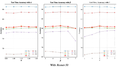
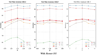
Figure 3: Sensitivity analysis of $\alpha$, $\beta$, $\tau$ with Resnet-50 (left) and Resnet-101 (right)

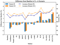
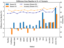
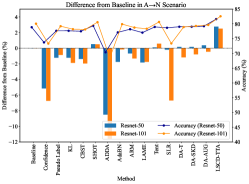
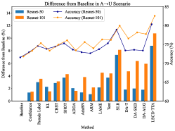
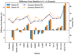
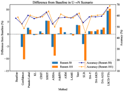
(a) Negative adaptation results with Resnet-50 and Resnet-101. Compared to other DA and TTA methods, it can be clearly seen that our proposed LSCD-TTA demonstrates state-of-the-art performances in adaptation tasks in terms of average accuracy.

V-C Ablation study on three loss designs

As shown in Tab. IV, we designed ablation experiments for the three studies. To ensure that it is the integrated validity of the loss module that is being explored, the experiments in this section all use the original optimal parameter settings (as shown in Fig. 3) and still uniformly use Resnet-50 and Resnet-101 [57] respectively as the network backbone. For convenience, the experiments use the average accuracy to assess the integrated validity of the model. In (A) and (B) experiments, we explore the effectiveness of $\mathcal{L}_{lsd}$ and $\mathcal{L}_{wcce}$ respectively. It is worth noting that the method using only $\mathcal{L}_{lsd}$ achieved the best performance of all the experiments in the N$\rightarrow$A task, and also showed a more prominent level of performance in the other tasks compared to the other methods in the Tab. III(a). At the meantime, the method using only $\mathcal{L}_{wcce}$ also exhibits a competitive performance. However, when we tried to consider the fusion of these two methods we found a slight decrease in performance. Although such a fusion approach highlights the high accuracy of the model, it lacks a certain level of robustness. For this reason, we consider replacing or introducing a third loss module $\mathcal{L}_{div}$, in the hope that it can further balance the fitness and accuracy of the adapted model during TTA process.

In experiments (C)-(E), we find that although the idea of combining $\mathcal{L}_{wcce}$ with $\mathcal{L}_{lsd}$ and $\mathcal{L}_{div}$ with $\mathcal{L}_{lsd}$ does not achieve the expected improvement, $\mathcal{L}_{lsd}$ combines with the third loss module $\mathcal{L}_{div}$ achieved better results in terms of average accuracy. Viewing the performance of different loss combinations in different DA tasks, we find that although they achieve a slight improvement in accuracy across these tasks relative to the performance of individual loss modules, they still do not provide a more balanced overall advantage. Therefore, we applied three loss modules simultaneously in experiment (F). Remarkably, when we applied the three loss modules simultaneously, we found that our proposed combined design LSCD-TTA achieves state-of-the-art results in most of the DA tasks. From an overall perspective, fully LSCD-TTA significantly improves the accuracy and stability in cross-scene remote sensing image classification tasks, indicating the superiority and robustness of our design.

V-D Sensitivity analysis of the hyperparameters $\alpha,\beta,\tau$

We find that the design of LSCD-TTA, which integrates three effective modules, consistently demonstrates state-of-the-art performance compared to advanced DA and TTA methods, regardless of different hyperparameter settings. However, the final performance of LSCD-TTA still exhibits slight fluctuations depending on the specific values of the hyperparameters. Accordingly, we conduct sensitivity studies on the hyperparameters $\alpha,\beta,\tau$ with different backbones separately to find the relatively best setting of the hyperparameter used in LSCD-TTA. To more visually compare the performance changes of different hyperparameter values in different DA tasks, we recorded the numerical result and plotted the change folds shown in tasks Fig. 3. In particular, since the absolute values calculated by the three loss designs are quite different, the scale and range of hyperparameter adjustments used for the three losses are also different. In order to prioritize achieving high basic performance for the model, we will begin by focusing on the $\mathcal{L}_{lsd}$ module, which demonstrated excellent performance in the ablation study. Initially, we will set a relatively small adjustment range for its hyperparameter $\alpha$, and then proceed to adjust the ranges of the other two hyperparameters to adapt to the adjusted $\mathcal{L}_{lsd}$.

Combining the graphical information, it can be learned that different hyperparameter values exhibit outstanding performance in various domain adaptation tasks respectively, while the overall distribution of advantages is more evenly distributed, each with its own merits. Nevertheless, it is certain that the model achieves the combined best performance when $\alpha=1.15,\beta=5,\tau=6$ with Resnet-50, as well as $\alpha=1.75,\beta=6,\tau=2$ with Resnet-101. Such an encouraged result demonstrates that our model strikes a notable balance between robustness and accuracy, wisely sacrificing an extremely slight amount of salient performance for a more comprehensive and significant increase in generalization ability.

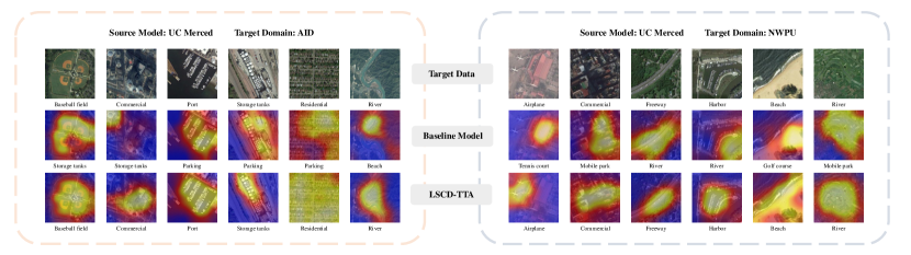
Figure 5: Grad-CAM Comparison between LSCD-TTA and Baseline model with Resnet-50. The calorific distribution shows the model’s inference concerns during different migration tasks, which reveals that the Baseline model is constrained by its limited knowledge when directly applied for target domain adaptation. It can be seen in incorrect attention (e.g., Commercial/Storage tanks in U$\rightarrow$A, Harbor/River in U$\rightarrow$N) and misclassification although at the true attention area (e.g., Port/Parking in U$\rightarrow$A, River/Freeway in U$\rightarrow$N). By contrast, LSCD-TTA rapidly adapts to the target domain during the testing phase, significantly enhancing the model’s attention performance and enabling fine-grained classification while preserving global semantic information.

VI Discussion

VI-A Negative transformer

To provide a more intuitive comparison of different methods against the baseline across various cross-domain remote sensing classification tasks, we calculated the average accuracy score between each method and the baseline with different backbones, and then plotted a negative transfer graph to compare the overall performance of different DA methods to the Baseline. As shown in Fig. 4(a), it is evident that LSCD-TTA consistently demonstrates state-of-the-art performance across nearly all domain adaptation tasks. Performance of our proposed LSCD-TTA is especially outstanding in U$\rightarrow$A and U$\rightarrow$N tasks, where the corresponding SD models are derived from a limited knowledge domain and faced with the much infomation-rich domains (as illustrated in Tab. I). Such phenomenons strongly indicate that the design of LSCD-TTA helps the model efficiently and robustly adapt to a broader and infomation-rich domain comprehensively.

Even noteworthy, while SLR [33] exhibits competitive performance in N$\rightarrow$A, N$\rightarrow$U and A$\rightarrow$U tasks, it exhibits unexpected negative transfer effects in the A$\rightarrow$N and U$\rightarrow$N DA tasks. In contrast to such fluctuating results across different tasks, LSCD-TTA produces more stable and consistent outcomes. It can also be verified that LSCD-TTA is tailored for remote sensing datasets with characteristics of numerous categories, high sample similarity and frequent data change, notably enhancing the performance in cross-domain classification tasks.

VI-B Model Visualization

In this section, we utilize Grad-CAM [64] to visually represent the model’s attention mechanisms. Grad-CAM generates a class-specific attention map by computing the gradient of the class score with respect to the feature maps produced by the convolutional layers. As shown in Fig. 5, such a phenomenon is especially evident when the model has only learned limited SD knowledge, as it tends to prioritize regions in the image that closely resemble the distribution of the SD priors (e.g., river and freeway, parking and port), which may lead to incorrect predictions easily. The design of LSCD-TTA allows the model to focus not only on maintaining classification accuracy for major samples but also on harder-to-classify cases. In short, LSCD-TTA flexibly adjusts the model’s receptive field, ensuring a balanced consideration of both global and local features.

VI-C Future outlook

Our approach delves into the application of TTA in remote sensing image classification, proposing strategies tailored to cross-scene classification tasks. LSCD-TTA includes loss function designs that address weak-category uncertainty and category diversity, alongside low saturation distribution loss to explore TD data distributions comprehensively. Through LSCD weighted module, our approach effectively addresses domain shifts and inconsistencies in data distribution, enhancing classification accuracy and generalization in the TD. Such a design definitely offers a practical solution for remote sensing image classification challenges, with potential significant impact on resource management, disaster monitoring, etc.

Although our proposed method achieves state-of-the-art results on three well-known open-source remote sensing image datasets, it is still limited by the inherent constraints of remote sensing image datasets, the TTA process, and UDA modes, which indicates a lot of room for LSCD-TTA in terms of future development. On the one hand, our method attempts to mitigate the domain adaptation problem through feature-aligned losses and domain offsets minimization, however, there are still some cases where the feature distributions are not well aligned in wider areas. It may lead to a degradation of the model’s performance on the TD, especially more notable in the face of large domain offsets. In the future, we plan to explore more effective feature alignment methods and domain adaptation strategies further to improve the model’s adaptability and generalization ability. On the other hand, We conduct TTA in which unsupervised learning is modeled, assuming one-to-one category correspondence between the source and target domains. However, in real-world cross-scene remote sensing image classification, the model often encounters entirely new categories due to the wide range of geographic environments covered. Accordingly, we plan to investigate further relevant methods in the future to improve the model’s ability to generalize to unknown domains and new knowledge.

VII Conclusion

In this paper, we propose a novel and comprehensive test-time adaptation (TTA) method for the cross-scene remote sensing image classification task: Low Saturation Confidence Distribution test-time adaptation (LSCD-TTA). LSCD-TTA is mainly designed for the feature loss functions of probability distributions in the source and target domains, within which low saturation distribution (LSD) enhances the performance of low-confidence samples in the later stages of TTA, weak-category cross-entropy (WCCE) improves the model’s ability to distinguish difficult-to-classify weak categories, and diverse categories confidence (DIV) softens the predicted probability distribution, which helps to better alleviate the deviation in cross-category sample distribution. To evaluate LSCD-TTA, we conduct comprehensive experiments on three well-known remote sensing image datasets (i.e., NWPU-RESISC45, AID, and UC Merced). LSCD-TTA achieves a significant increase of 4.96$\%$-10.51$\%$ with Resnet-50 and 5.33$\%$-12.49$\%$ with Resnet-101 in average accuracy compared to other state-of-the-art DA and TTA methods, and also achieves quite competitive performance in robust evaluation metrics such as variance. The experimental results show that LSCD-TTA achieves outstanding results in solving the cross-scene classification task on remote sensing image data, which empowers the source model to generalize quickly and accurately. Accordingly, we believe that LSCD-TTA will have a broad prospect in more practical and generalized DA scenarios in remote sensing community.

References

- [1] Y. Li, Y. Zhang, and Z. Zhu, “Learning deep networks under noisy labels for remote sensing image scene classification,” in IGARSS 2019-2019 IEEE International Geoscience and Remote Sensing Symposium. IEEE, 2019, pp. 3025–3028.
- [2] W. Teng, N. Wang, H. Shi et al., “Classifier-constrained deep adversarial domain adaptation for cross-domain semisupervised classification in remote sensing images,” IEEE Geoscience and Remote Sensing Letters, vol. 17, no. 5, pp. 789–793, 2019.
- [3] S. Dong, Y. Zhuang, Z. Yang, L. Pang et al., “Land cover classification from vhr optical remote sensing images by feature ensemble deep learning network,” IEEE Geoscience and Remote Sensing Letters, vol. 17, no. 8, pp. 1396–1400, 2019.
- [4] J. Zheng, S. Yuan, W. Wu, W. Li, L. Yu, H. Fu, and D. Coomes, “Surveying coconut trees using high-resolution satellite imagery in remote atolls of the pacific ocean,” Remote Sensing of Environment, vol. 287, p. 113485, 2023.
- [5] Y. Ganin and V. Lempitsky, “Unsupervised domain adaptation by backpropagation,” in International conference on machine learning. PMLR, 2015, pp. 1180–1189.
- [6] C. Ma, D. Sha, and X. Mu, “Unsupervised adversarial domain adaptation with error-correcting boundaries and feature adaption metric for remote-sensing scene classification,” Remote Sensing, vol. 13, no. 7, p. 1270, 2021.
- [7] L. Ma et al., “Centroid and covariance alignment-based domain adaptation for unsupervised classification of remote sensing images,” IEEE Transactions on Geoscience and Remote Sensing, vol. 57, no. 4, pp. 2305–2323, 2018.
- [8] Q. Li, Y. Wen, J. Zheng, Y. Zhang, and H. Fu, “Hyunida: Breaking label set constraints for universal domain adaptation in cross-scene hyperspectral image classification,” IEEE Transactions on Geoscience and Remote Sensing, 2024.
- [9] J. Zheng, Y. Wen, M. Chen, S. Yuan, W. Li, Y. Zhao, W. Wu et al., “Open-set domain adaptation for scene classification using multi-adversarial learning,” ISPRS Journal of Photogrammetry and Remote Sensing, vol. 208, pp. 245–260, 2024.
- [10] D. Hou et al., “Pcluda: A pseudo-label consistency learning-based unsupervised domain adaptation method for cross-domain optical remote sensing image retrieval,” IEEE Transactions on Geoscience and Remote Sensing, vol. 61, pp. 1–14, 2022.
- [11] E. Capliez, D. Ienco, R. Gaetano, and N. a. Baghdadi, “Multi-sensor temporal unsupervised domain adaptation for land cover mapping with spatial pseudo labelling and adversarial learning,” IEEE Transactions on Geoscience and Remote Sensing, 2023.
- [12] Y. Liang, R. Huang, X. Li, J. Yang, X. Zhang, and X. Wang, “Adaptive federated learning for electric power inspection with uav system.” in ICCEIC, 2022, pp. 234–241.
- [13] J. N. Kundu, N. Venkat et al., “Universal source-free domain adaptation,” in Proceedings of the IEEE/CVF conference on computer vision and pattern recognition, 2020, pp. 4544–4553.
- [14] D.-H. Lee et al., “Pseudo-label: The simple and efficient semi-supervised learning method for deep neural networks,” in Workshop on challenges in representation learning, ICML, vol. 3, no. 2. Atlanta, 2013, p. 896.
- [15] T. Chen, S. Kornblith et al., “A simple framework for contrastive learning of visual representations,” in International conference on machine learning. PMLR, 2020, pp. 1597–1607.
- [16] I. Goodfellow et al., “Generative adversarial nets,” Advances in neural information processing systems, vol. 27, 2014.
- [17] N. Jiang, H.-B. Li, C.-J. Li, H.-X. Xiao, and J.-W. Zhou, “A fusion method using terrestrial laser scanning and unmanned aerial vehicle photogrammetry for landslide deformation monitoring under complex terrain conditions,” IEEE Transactions on Geoscience and Remote Sensing, vol. 60, pp. 1–14, 2022.
- [18] D. Wang, E. Shelhamer, S. Liu, B. Olshausen, and T. Darrell, “Tent: Fully test-time adaptation by entropy minimization,” arXiv preprint arXiv:2006.10726, 2020.
- [19] M. Boudiaf, R. Mueller, I. Ben Ayed, and L. Bertinetto, “Parameter-free online test-time adaptation,” in Proceedings of the IEEE/CVF Conference on Computer Vision and Pattern Recognition, 2022, pp. 8344–8353.
- [20] D. Hendrycks and T. Dietterich, “Benchmarking neural network robustness to common corruptions and perturbations,” arXiv preprint arXiv:1903.12261, 2019.
- [21] S. Lee, D. Kim, N. Kim, and S.-G. Jeong, “Drop to adapt: Learning discriminative features for unsupervised domain adaptation,” in Proceedings of the IEEE/CVF international conference on computer vision, 2019, pp. 91–100.
- [22] J. Zhang, J. Huang, Z. Tian, and S. Lu, “Spectral unsupervised domain adaptation for visual recognition,” in Proceedings of the IEEE/CVF Conference on Computer Vision and Pattern Recognition, 2022, pp. 9829–9840.
- [23] G. Wei, C. Lan et al., “Metaalign: Coordinating domain alignment and classification for unsupervised domain adaptation,” in Proceedings of the IEEE/CVF conference on computer vision and pattern recognition, 2021, pp. 16 643–16 653.
- [24] Q. Wang and T. Breckon, “Unsupervised domain adaptation via structured prediction based selective pseudo-labeling,” in Proceedings of the AAAI conference on artificial intelligence, vol. 34, no. 04, 2020, pp. 6243–6250.
- [25] J. Wang and X.-L. Zhang, “Improving pseudo labels with intra-class similarity for unsupervised domain adaptation,” Pattern Recognition, vol. 138, p. 109379, 2023.
- [26] N. Ding, Y. Xu, Y. Tang, C. Xu, Y. Wang, and D. Tao, “Source-free domain adaptation via distribution estimation,” in Proceedings of the IEEE/CVF conference on computer vision and pattern recognition, 2022, pp. 7212–7222.
- [27] M. Litrico, A. Del Bue, and P. Morerio, “Guiding pseudo-labels with uncertainty estimation for source-free unsupervised domain adaptation,” in Proceedings of the IEEE/CVF Conference on Computer Vision and Pattern Recognition, 2023, pp. 7640–7650.
- [28] S. Yang, Y. Wang et al., “Generalized source-free domain adaptation,” in Proceedings of the IEEE/CVF international conference on computer vision, 2021, pp. 8978–8987.
- [29] Y. Liu, Y. Chen, W. Dai, M. Gou et al., “Source-free domain adaptation with contrastive domain alignment and self-supervised exploration for face anti-spoofing,” in European Conference on Computer Vision. Springer, 2022, pp. 511–528.
- [30] S. Tang, W. Su, M. Ye, and X. Zhu, “Source-free domain adaptation with frozen multimodal foundation model,” in Proceedings of the IEEE/CVF Conference on Computer Vision and Pattern Recognition, 2024, pp. 23 711–23 720.
- [31] Y. Mitsuzumi et al., “Understanding and improving source-free domain adaptation from a theoretical perspective,” in Proceedings of the IEEE/CVF Conference on Computer Vision and Pattern Recognition, 2024, pp. 28 515–28 524.
- [32] M. Zhang, S. Levine, and C. Finn, “Memo: Test time robustness via adaptation and augmentation,” Advances in neural information processing systems, vol. 35, pp. 38 629–38 642, 2022.
- [33] C. K. Mummadi, R. Hutmacher, K. Rambach, E. Levinkov, T. Brox, and J. H. Metzen, “Test-time adaptation to distribution shift by confidence maximization and input transformation,” arXiv preprint arXiv:2106.14999, 2021.
- [34] J. Ma, “Improved self-training for test-time adaptation,” in Proceedings of the IEEE/CVF Conference on Computer Vision and Pattern Recognition, 2024, pp. 23 701–23 710.
- [35] S. Wang, D. Zhang, Z. Yan, J. Zhang, and R. Li, “Feature alignment and uniformity for test time adaptation,” in Proceedings of the IEEE/CVF Conference on Computer Vision and Pattern Recognition, 2023, pp. 20 050–20 060.
- [36] S. Choi, S. Yang, S. Choi, and S. Yun, “Improving test-time adaptation via shift-agnostic weight regularization and nearest source prototypes,” in European Conference on Computer Vision. Springer, 2022, pp. 440–458.
- [37] Y. Feng, X. Xu, H. Fu, Y. Wang, Z. Wang et al., “Category-aware test-time training domain adaptation,” in 2024 IEEE Conference on Artificial Intelligence (CAI). IEEE, 2024, pp. 300–306.
- [38] H. Yang et al., “Dltta: Dynamic learning rate for test-time adaptation on cross-domain medical images,” IEEE Transactions on Medical Imaging, vol. 41, no. 12, pp. 3575–3586, 2022.
- [39] M. Zhang, H. Marklund et al., “Adaptive risk minimization: Learning to adapt to domain shift,” Advances in Neural Information Processing Systems, vol. 34, pp. 23 664–23 678, 2021.
- [40] X. Ruan and W. Tang, “Fully test-time adaptation for object detection,” in Proceedings of the IEEE/CVF Conference on Computer Vision and Pattern Recognition, 2024, pp. 1038–1047.
- [41] S. Niu, J. Wu et al., “Towards stable test-time adaptation in dynamic wild world,” arXiv preprint arXiv:2302.12400, 2023.
- [42] J. Guo, Y. Lai, J. Zhang et al., “C 3 da: A universal domain adaptation method for scene classification from remote sensing imagery,” IEEE Geoscience and Remote Sensing Letters, 2024.
- [43] P. Shamsolmoali, M. Zareapoor, H. Zhou, R. Wang, and J. Yang, “Road segmentation for remote sensing images using adversarial spatial pyramid networks,” IEEE Transactions on Geoscience and Remote Sensing, vol. 59, no. 6, pp. 4673–4688, 2020.
- [44] Y. Li, T. Shi, Y. Zhang, W. Chen, Z. Wang, and H. Li, “Learning deep semantic segmentation network under multiple weakly-supervised constraints for cross-domain remote sensing image semantic segmentation,” ISPRS Journal of Photogrammetry and Remote Sensing, vol. 175, pp. 20–33, 2021.
- [45] J. Zheng, H. Fu, W. Li, W. Wu, Y. Zhao et al., “Cross-regional oil palm tree counting and detection via a multi-level attention domain adaptation network,” ISPRS Journal of Photogrammetry and Remote Sensing, vol. 167, pp. 154–177, 2020.
- [46] W. Wu, J. Zheng et al., “Cross-regional oil palm tree detection,” in Proceedings of the IEEE/CVF Conference on Computer Vision and Pattern Recognition Workshops, 2020, pp. 56–57.
- [47] J. Zheng, W. Wu, S. Yuan, H. Fu, W. Li, and L. Yu, “Multisource-domain generalization-based oil palm tree detection using very-high-resolution (vhr) satellite images,” IEEE Geoscience and Remote Sensing Letters, vol. 19, pp. 1–5, 2021.
- [48] H. Zuo et al., “Multiple-source domain adaptation in rule-based neural network,” in 2020 International Joint Conference on Neural Networks (IJCNN). IEEE, 2020, pp. 1–6.
- [49] C. Geiß, H. Schrade, P. A. Pelizari, and H. Taubenböck, “Multistrategy ensemble regression for mapping of built-up density and height with sentinel-2 data,” ISPRS Journal of Photogrammetry and Remote Sensing, vol. 170, pp. 57–71, 2020.
- [50] Z. Xu, W. Wei, L. Zhang, and J. Nie, “Source-free domain adaptation for cross-scene hyperspectral image classification,” in IGARSS 2022-2022 IEEE International Geoscience and Remote Sensing Symposium. IEEE, 2022, pp. 3576–3579.
- [51] W. Liu, J. Liu, X. Su, H. Nie, and B. Luo, “Source-free domain adaptive object detection in remote sensing images,” arXiv preprint arXiv:2401.17916, 2024.
- [52] G.-S. Xia, J. Hu, F. Hu, B. Shi, X. Bai, Y. Zhong, L. Zhang, and X. Lu, “Aid: A benchmark data set for performance evaluation of aerial scene classification,” IEEE Transactions on Geoscience and Remote Sensing, vol. 55, no. 7, pp. 3965–3981, 2017.
- [53] G. Cheng, J. Han, and X. Lu, “Remote sensing image scene classification: Benchmark and state of the art,” Proceedings of the IEEE, vol. 105, no. 10, pp. 1865–1883, 2017.
- [54] Y. Yang and S. Newsam, “Bag-of-visual-words and spatial extensions for land-use classification,” in Proceedings of the 18th SIGSPATIAL international conference on advances in geographic information systems, 2010, pp. 270–279.
- [55] J. Zheng, W. Wu, S. Yuan, Y. Zhao, W. Li, L. Zhang et al., “A two-stage adaptation network (tsan) for remote sensing scene classification in single-source-mixed-multiple-target domain adaptation (s2m2t da) scenarios,” IEEE Transactions on Geoscience and Remote Sensing, vol. 60, pp. 1–13, 2021.
- [56] J. Zheng, Y. Zhao et al., “Partial domain adaptation for scene classification from remote sensing imagery,” IEEE Transactions on Geoscience and Remote Sensing, vol. 61, pp. 1–17, 2022.
- [57] K. He, X. Zhang, S. Ren, and J. Sun, “Deep residual learning for image recognition,” in Proceedings of the IEEE conference on computer vision and pattern recognition, 2016, pp. 770–778.
- [58] S. Kullback et al., “On information and sufficiency,” The annals of mathematical statistics, vol. 22, no. 1, pp. 79–86, 1951.
- [59] Y. Zou, Z. Yu, B. Kumar, and J. Wang, “Unsupervised domain adaptation for semantic segmentation via class-balanced self-training,” in Proceedings of the European conference on computer vision (ECCV), 2018, pp. 289–305.
- [60] E. Tzeng, J. Hoffman et al., “Adversarial discriminative domain adaptation,” in Proceedings of the IEEE conference on computer vision and pattern recognition, 2017, pp. 7167–7176.
- [61] J. Liang, D. Hu, and J. Feng, “Do we really need to access the source data? source hypothesis transfer for unsupervised domain adaptation,” in International conference on machine learning. PMLR, 2020, pp. 6028–6039.
- [62] J. Zhang, L. Qi et al., “Domainadaptor: A novel approach to test-time adaptation,” in Proceedings of the IEEE/CVF International Conference on Computer Vision, 2023, pp. 18 971–18 981.
- [63] Y. Li et al., “Adaptive batch normalization for practical domain adaptation,” Pattern Recognition, vol. 80, pp. 109–117, 2018.
- [64] R. R. Selvaraju, M. Cogswell, A. Das, R. Vedantam et al., “Grad-cam: Visual explanations from deep networks via gradient-based localization,” in Proceedings of the IEEE international conference on computer vision, 2017, pp. 618–626.