Cosmological Stasis from a Single Annihilating Particle Species:
Extending Stasis Into the Thermal Domain

Abstract

It has recently been shown that extended cosmological epochs can exist during which the abundances associated with different energy components remain constant despite cosmological expansion. Indeed, this “stasis” behavior has been found to arise generically in many BSM theories containing large towers of states, and even serves as a cosmological attractor. However, all previous studies of stasis took place within non-thermal environments, or more specifically within environments in which thermal effects played no essential role in realizing or sustaining the stasis. In this paper, we demonstrate that stasis can emerge and serve as an attractor even within thermal environments, with thermal effects playing a critical role in the stasis dynamics. Moreover, within such environments, we find that no towers of states are needed — a single state experiencing two-body annihilations will suffice. This work thus extends the stasis phenomenon into the thermal domain and demonstrates that thermal effects can also generally give rise to an extended stasis epoch, even when only a single matter species is involved.

I Introduction

It has recently been observed that many theories of physics beyond the Standard Model (BSM) give rise to early-universe cosmologies which potentially contain extended epochs during which the abundances of different cosmological energy components (such as matter, radiation, and vacuum energy) remain constant despite cosmological expansion. This phenomenon has been dubbed “stasis” Dienes et al. (2022a), and seems to be rather ubiquitous in systems containing large (or even infinite) towers of increasingly massive states, such as are known to arise in many BSM models Barrow et al. (1991); Dienes et al. (2022a, b, 2023, 2024); Halverson and Pandya (2024). Indeed, it has been found that matter and radiation can be in stasis with each other Dienes et al. (2022a); Barrow et al. (1991); Dienes et al. (2022b); Halverson and Pandya (2024), and that each of these can also be in stasis with vacuum energy Dienes et al. (2023, 2024). It has even been found that matter, radiation, and vacuum energy can all experience a simultaneous triple stasis Dienes et al. (2023). Moreover, stasis is a dynamical attractor within such cosmologies. Thus, even if these systems do not begin in stasis, they will naturally flow towards such stasis configurations. This renders the stasis state essentially unavoidable in many BSM cosmologies.

All of the BSM cosmologies which have been examined thus far share certain characteristics. First, they are all non-thermal. By this, we mean that they do not involve any cosmological energy components whose temperatures play a critical role in the stasis phenomenon. Even in cases for which the stasis is realized through the Hawking radiation emitted by primordial black holes Barrow et al. (1991); Dienes et al. (2022b), it is sufficient to regard the black-hole evaporation process as one which simply converts matter (in the form of black holes) to radiation. In such analyses — indeed, in all of the different stasis scenarios examined thus far — the temperatures that might happen to characterize particular cosmological populations of particles play no essential role in the stasis dynamics. Secondly, and perhaps even more importantly, in all of the BSM systems examined thus far the existence of a bona fide tower of different species $\phi_{\ell}$ with different masses $m_{\ell}$ was critical. Indeed, we have even repeatedly found that the duration of the resulting stasis epoch is directly related to the number of species in the tower. Finally — and a bit more technically — the energy-transfer mechanisms that drove the stasis phenomenon in each of the previous cases (such as the decay of matter to radiation in Refs. Dienes et al. (2022a); Barrow et al. (1991); Dienes et al. (2023), or the transition from overdamped fields to underdamped fields in Refs. Dienes et al. (2023, 2024)) had the property that the rate of energy transfer depended linearly on the energy density associated with the original field. More specifically, the “pumps” $P^{(\rho)}$ that were required in each of the previous cases were each proportional to $\rho$. This linearity property played a significant role in establishing the algebraic structure of the resulting stasis. While suitable for decay processes in which a matter particle $\phi$ decays into radiation, thereby leading to a rate of energy transfer from matter to radiation scaling linearly with the $\phi$-particle density $n_{\phi}$, this linearity property would seem to preclude processes such as particle annihilation, for which we would expect a rate that scales as $n_{\phi}^{2}$.

Given these observations, one might suspect that each of these features plays a necessary role in establishing the stasis phenomenon. However, in this paper, we shall demonstrate that none of these features are actually required for stasis. In particular, we shall describe an explicit thermal scenario which has none of the features outlined above, but which nevertheless is capable of producing an epoch of stasis persisting across many e-folds of cosmological expansion. Indeed, we shall even show that such a stasis epoch is a cosmological attractor.

As might be imagined, the thermal stasis that we shall describe in this paper is quite different from the non-thermal stases that already exist in the literature. Without a tower of states, and with the stasis driven by particle annihilation rather than by particles decaying or undergoing phase transitions, it might seem at first glance that thermal stasis must emerge in a completely different way. Indeed, even the pumps that we shall employ in this paper may be more familiar from studies of thermal freezeout in weakly-interacting-massive-particle (WIMP) models of dark matter than from prior studies of stasis. However, despite these important differences, we shall nevertheless find that a stasis likewise emerges within this new context and shares many critical properties with its non-thermal cousins.

This paper is organized as follows. In Sect. II, we describe the different cosmological energy components that will be present in our thermal-stasis framework. We also discuss the fundamental assumptions regarding the manner in which they behave. As we shall see, one of these components is a population of non-relativistic particles which are in kinetic equilibrium with each other. Then, in Sect. III, we derive the evolution equations not only for the cosmological abundances of our energy components but also for the temperature of this non-relativistic particle gas. In Sect. IV, we examine the general forms of the pump terms that arise in these equations due to the annihilation of our non-relativistic particles. In Sect. V, we then proceed to identify a particular combination of our dynamical variables — a combination which we call “coldness” — which plays a crucial role in the cosmological dynamics, and we recast our evolution equations in terms of this new variable. In Sect. VI we examine the fixed-point solutions to these equations, and demonstrate that a novel form of stasis emerges as such a fixed point under certain conditions. Indeed, we shall find that it is the coldness rather than the temperature which remains constant during thermal stasis. In Sect. VII, we demonstrate that this stasis solution is not merely a local attractor, but actually a global attractor when these conditions are satisfied. In Sect. VIII, we then identify a particular mechanism through which these stasis conditions can naturally be realized in a particle-physics context. Finally, in Sect. IX, we conclude with a summary of our results and a discussion highlighting possible directions for future work.

II Assumptions and Energy Components

In this paper, our goal is to study the extent to which stasis can emerge in a thermal environment. Toward this end, in this section we shall begin by describing the cosmological energy components present in our framework for establishing such a stasis and the fundamental assumptions regarding the manner in which they behave. For sake of generality, we shall keep the discussion as model-independent as possible in what follows. Later, in Sect. VIII, we shall present an explicit mechanism through which these conditions can be realized in a particle-physics context.

Let us start by considering the cosmology associated with a universe which comprises a non-relativistic matter species $\phi$ of mass $m$ which annihilates into an effectively massless particle $\chi$ through processes of the form $\phi\phi\to\chi\chi$. For simplicity, we shall assume that $\phi$ and $\chi$ are both their own antiparticles (although our qualitative results would be unchanged if we were to drop this last assumption). Thus, such a universe contains not only a matter component $\phi$ with an energy density $\rho_{M}$, abundance $\Omega_{M}$, and equation-of-state parameter $w_{M}=0$, but also a radiation component $\chi$ with a corresponding energy density $\rho_{\gamma}$, abundance $\Omega_{\gamma}$, and equation-of-state parameter $w_{\gamma}=1/3$. For simplicity, we shall assume that these matter and radiation components are the only cosmological energy components present within our universe, and that the universe is flat and expanding in a manner consistent with the FRW metric.

Remarkably, we shall demonstrate that such a universe can give rise to an extended stasis epoch. To do this, we shall assume that our population of matter particles comprises only a single species $\phi$ with a unique mass $m$. We shall also assume that this species is stable in the sense that it does not decay within the time frame relevant for our analysis. Finally, we shall assume that the $\phi$ particles are not absolutely cold, but rather are in thermal equilibrium with each other, possibly as the result of rapid interactions among them, and constitute an ideal gas with a non-zero temperature $T$.

Note that our assumption that the $\phi$ particles form an ideal gas does not imply the existence of a thermal bath which holds the temperature of this gas constant. Rather, we shall allow the temperature of our $\phi$-particle gas to evolve dynamically along with the rest of the cosmology. In other words, while we will assume the existence of rapid interactions amongst the $\phi$ particles which ensure that they remain in thermal equilibrium with each other, we are not assuming that these particles have additional interactions with any other particle species that might have constituted a thermal bath.

Given these assumptions, we see that we must actually regard our universe as containing three different “fluids”. The first two fluids are those mentioned above, namely those associated with matter and radiation, but our matter fluid really only accounts for the rest-mass energy of our matter fields. We must therefore now introduce a third fluid, namely that associated with the kinetic energy of our matter fields, with corresponding energy density $\rho_{\rm KE}$, abundance $\Omega_{\rm KE}$, and equation-of-state parameter $w_{\rm KE}$. It is important to note that we cannot consider $\rho_{M}$ and $\rho_{\rm KE}$ as different contributors to a single common fluid associated with our gas of $\phi$ particles with a unique time-independent equation of state of the form $P=w\rho$ with a constant $w$, since (as we shall demonstrate below) the energy densities associated with rest mass and kinetic energy have different equations of state of this form, with $w_{M}\not=w_{\rm KE}$.

Since we are assuming that our $\phi$ particles constitute a non-relativistic ideal gas at temperature $T$, it follows that $\rho_{\rm KE}$ and $T$ are related to each other via

$$\rho_{\rm KE}~{}=~{}\frac{3}{2}n_{M}T~{}\approx~{}\frac{3}{2}\rho_{M}\frac{T}{m}~{},$$ (1)

where $n_{M}\approx\rho_{M}/m$ is the number density of $\phi$ particles in the gas. The kinetic-energy abundance is therefore

$$\Omega_{\rm KE}~{}=~{}\frac{3}{2}\Omega_{M}\frac{T}{m}~{}.$$ (2)

Thus, for a given $\Omega_{M}$, we can trade $\Omega_{\rm KE}$ for $T$ and vice versa.

We can also define an equation-of-state parameter $w_{\rm KE}$ for the kinetic energy of our $\phi$-particle gas. The ideal gas law tells us that $P=n_{M}T$, where $P$ is the total pressure associated with this gas. It then follows from Eq. (1) that $\rho_{\rm KE}=3P/2$, which implies that

$$w_{\rm KE}~{}=~{}\frac{2}{3}~{}.$$ (3)

Another way to understand this result is to consider how the kinetic-energy density of our $\phi$ particles scales with the scale factor $a$. In general, the kinetic-energy density of a localized population of particles in a FRW universe always includes a factor $a^{-3}$ due to the expansion of the volume within which those particles are contained. However, this kinetic-energy density may also accrue an additional dependence on $a$ from the manner in which the kinetic energies of the individual particles are affected by the redshifting of their momenta. For example, if the particle is highly relativistic, its kinetic energy is approximately proportional to its momentum $p$ and therefore scales as $a^{-1}$. Thus, the kinetic-energy density of a population of such a particles — which is essentially equivalent to their total energy density — scales as $a^{-4}$. Since we generally have $\rho\sim a^{-3(1+w)}$ for a perfect fluid with a constant equation-of-state parameter $w$, we obtain the usual result $w=1/3$ for radiation. By contrast, the kinetic energy associated with a non-relativistic particle is proportional to $p^{2}$ and therefore scales as $a^{-2}$. Thus, the kinetic-energy density of a population of non-relativistic particles scales as $a^{-5}$. This corresponds to an equation-of-state parameter $w=2/3$, in accordance with Eq. (3).

III Dynamical Equations

It is now relatively straightforward to derive the equations that govern the time-evolution of the three abundances $\Omega_{M}$, $\Omega_{\gamma}$, and $\Omega_{\rm KE}$ within this cosmology. Each of these abundances $\Omega_{i}$ is related to the corresponding energy density $\rho_{i}$ via

$$\Omega_{i}~{}\equiv~{}\frac{8\pi G}{3H^{2}}\,\rho_{i}~{}~{}$$ (4)

where $i\in\{M,\gamma,{\rm KE}\}$, where $H\equiv\dot{a}/a$ is the Hubble parameter, and where $G$ is Newton’s constant. It then follows that

$$\frac{d\Omega_{i}}{dt}~{}=~{}\frac{8\pi G}{3}\left(\frac{1}{H^{2}}\frac{d\rho_{i}}{dt}-2\frac{\rho_{i}}{H^{3}}\frac{dH}{dt}\right)~{}.$$ (5)

On the other hand, for our three-component universe, the Friedmann acceleration equation tells us that

$$\frac{dH}{dt}~{} = ~{}-H^{2}-\frac{4\pi G}{3}\left(\sum_{i}\rho_{i}+3\sum_{i}p_{i}\right)$$

$$= ~{}-{\textstyle{1\over 2}}H^{2}\left(2+\Omega_{M}+2\Omega_{\gamma}+3\Omega_{\rm KE}\right)$$

$$= ~{}-{\textstyle{1\over 2}}H^{2}\left(4-\Omega_{M}+\Omega_{\rm KE}\right)~{}$$ (6)

where in passing from the second to the third line we have imposed the constraint $\Omega_{M}+\Omega_{\gamma}+\Omega_{\rm KE}=1$, as befits our three-component universe. Substituting Eq. (6) into Eq. (5) then yields

$$\frac{d\Omega_{M}}{dt}~{} = ~{}\frac{8\pi G}{3H^{2}}\,\frac{d\rho_{M}}{dt}+H\Omega_{M}\left(4-\Omega_{M}+\Omega_{\rm KE}\right)~{}$$

$$\frac{d\Omega_{\gamma}}{dt}~{} = ~{}\frac{8\pi G}{3H^{2}}\,\frac{d\rho_{\gamma}}{dt}+H\Omega_{\gamma}\left(4-\Omega_{M}+\Omega_{\rm KE}\right)~{}$$

$$\frac{d\Omega_{\rm KE}}{dt}~{} = ~{}\frac{8\pi G}{3H^{2}}\,\frac{d\rho_{\rm KE}}{dt}+H\Omega_{\rm KE}\left(4-\Omega_{M}+\Omega_{\rm KE}\right)~{}.~{}$$

In general, the rates of change $d\rho_{M}/dt$, $d\rho_{\gamma}/dt$, and $d\rho_{\rm KE}/dt$ of the energy densities associated with our three cosmological components may be written schematically as

$$\frac{d\rho_{M}}{dt}~{} = ~{}-3H\rho_{M}-P^{(\rho)}_{M,\gamma}~{}$$

$$\frac{d\rho_{\gamma}}{dt}~{} = ~{}-4H\rho_{\gamma}+P^{(\rho)}_{M,\gamma}+P^{(\rho)}_{{\rm KE},\gamma}~{}$$

$$\frac{d\rho_{\rm KE}}{dt}~{} = ~{}-5H\rho_{\rm KE}-P^{(\rho)}_{{\rm KE},\gamma}~{},$$ (8)

where the first term on the right side of each equation represents the effect of cosmological expansion and where each of the remaining terms $P^{(\rho)}_{ij}$ represents the rate at which energy-density is transferred from component $i$ to component $j$ as a consequence of our annihilation process $\phi\phi\to\chi\chi$. In general, this annihilation process eliminates $\phi$ particles and thereby reduces not only the rest-mass energy density $\rho_{M}$ of the $\phi$-particle gas but also its kinetic energy density $\rho_{\rm KE}$. The fact that this process conserves energy then implies that any annihilation-induced reductions in $\rho_{M}$ and $\rho_{\rm KE}$ must lead to a corresponding increase in $\rho_{\gamma}$.

Note that we have not included similar terms for the inverse process $\chi\chi\to\phi\phi$ in Eq. (8). However, the energy-density-transfer rates associated with this process are generally negligible within our primary regime of interest. To see this, we begin by noting that since our gas of $\phi$ particles is presumed to be highly non-relativistic, the energies $E_{\chi}$ of the $\chi$ particles produced by $\phi\phi\to\chi\chi$ annihilation at any given time are initially sharply peaked around $E_{\chi}\sim m$ in the cosmological background frame, with a width $\Delta E_{\chi}\sim\sqrt{mT}\ll m$ where $T$ is the temperature of the $\phi$-particle gas at that time. However, these energies subsequently decrease as a result of cosmological redshifting. In situations in which the $\chi$ particles interact sufficiently weakly that little redistribution of the $E_{\chi}$ takes place after they are produced, these energies quickly fall below the kinematic threshold for $\chi\chi\to\phi\phi$ production. Even in situations in which the $\chi$ particles are more strongly interacting and a more significant redistribution of $E_{\chi}$ values takes place, only a small (and ever-decreasing) fraction of $\chi$-particle pairs will ultimately have energies above this threshold. In either case, then, cosmological redshifting effectively renders the swept-volume rate for $\chi\chi\to\phi\phi$ production negligible.

We also note that while the scattering process $\chi\phi\to\chi\phi$ can in principle affect the distribution of kinetic energies for the $\phi$-particle gas, the swept-volume rate for this process need not be comparable to the swept-volume rate for $\phi\phi\to\chi\chi$ annihilation. For example, if $\phi\phi\to\chi\chi$ annihilation were to proceed through an $s$-channel process which occurs on resonance while simultaneously $\chi\phi\to\chi\phi$ were to occur only through $t$-channel processes, the swept-volume rate for the former process could be significant while that for the latter process could be sufficiently small that its impact on the dynamical evolution of the system could be neglected. Indeed, as we shall see in Sect. VIII, there exist scenarios for thermal stasis in which this is in fact the case. We shall therefore assume in what follows that the effect of $\chi\phi\to\chi\phi$ scattering on the kinetic-energy distribution of the $\phi$ particles can be neglected.

In general, following Ref. Dienes et al. (2023), we shall refer to any process that induces a transfer of energy between two energy components as a “pump.” Such pumps are associated with local particle-physics processes which conserve energy density, but redistribute it among our different energy components.

Substituting the expressions in Eq. (8) into Eq. (LABEL:convert2), we have

$$\frac{d\Omega_{M}}{dt}~{} = ~{}H\Omega_{M}\left(1-\Omega_{M}+\Omega_{\rm KE}\right)~{}-P_{M,\gamma}$$

$$\frac{d\Omega_{\gamma}}{dt}~{} = ~{}H\Omega_{\gamma}\left(-\Omega_{M}+\Omega_{\rm KE}\right)+P_{M,\gamma}+P_{{\rm KE},\gamma}~{}$$

$$\frac{d\Omega_{\rm KE}}{dt}~{} = ~{}H\Omega_{\rm KE}\left(-1-\Omega_{M}+\Omega_{\rm KE}\right)~{}-P_{{\rm KE},\gamma}~{},~{}~{}~{}~{}~{}$$ (9)

where we have defined

$$P_{ij}~{}\equiv~{}\frac{8\pi G}{3H^{2}}\,P^{(\rho)}_{ij}~{}.$$ (10)

Indeed, while the pump term $P^{(\rho)}_{ij}$ represents a transfer of energy density, the corresponding pump term $P_{ij}$ represents a transfer of abundance. We observe from Eq. (9) that $d\Omega_{M}/dt+d\Omega_{\gamma}/dt+d\Omega_{\rm KE}/dt=0$, which reflects the fact that $\Omega_{M}+\Omega_{\gamma}+\Omega_{\rm KE}=1$ within this three-component universe. For this reason, we shall henceforth refrain from writing down explicit expressions for $d\Omega_{\gamma}/dt$, as these expressions can always be determined directly from $d\Omega_{M}/dt$ and $d\Omega_{\rm KE}/dt$.

From our result for $d\Omega_{\rm KE}/dt$ in Eq. (9) and the relation in Eq. (2), we may also obtain an expression for the rate of change of the temperature of the $\phi$ particles. This expression takes the form

$$\frac{dT}{dt}~{}=~{}-2HT-\frac{2m}{3\Omega_{M}}\left(P_{{\rm KE},\gamma}-\frac{\Omega_{\rm KE}}{\Omega_{M}}\,P_{M,\gamma}\right)~{}.$$ (11)

This result implies that while the pump terms $P_{{\rm KE},\gamma}$ and $P_{M,\gamma}$ both serve to decrease the overall energy density associated with our $\phi$-particle gas, the former term serves to decrease its temperature while the latter serves to increase it. Indeed, we observe that the net effect of the pumps is to raise $T$ when

$$\frac{P_{{\rm KE},\gamma}}{\Omega_{\rm KE}}~{}<~{}\frac{P_{M,\gamma}}{\Omega_{M}}~{},$$ (12)

and to lower $T$ if the opposite is true. Interestingly, if both sides of Eq. (12) are equal, these pumps will have no net effect on $T$. Of course, $T$ still decreases as a consequence of cosmological expansion in this case, as indicated by the first term on the right side of Eq. (11).

IV Pump Terms for Thermal Annihilation

It is not difficult to obtain explicit expressions for our pump terms. Within the cosmology we are studying, such pumps represent the effects of the two-body annihilations of $\phi$ particles into radiation. Such process are familiar from traditional studies of the thermal freezeout phenomenon, where one has $dn_{M}/dt\sim\langle\sigma v\rangle n_{M}^{2}+...$ where $n_{M}$ is the matter-particle number density. In this expression, $\langle\sigma v\rangle$ denotes the thermally averaged “swept-volume” rate, i.e., the rate at which volume is swept by the cross-section $\sigma$ moving with transverse velocity $v$. Recognizing that $n_{M}=\rho_{M}/m$, we see that our corresponding pump is nothing but

$$P^{(\rho)}_{M,\gamma}~{}=~{}\frac{1}{m}\langle\sigma v\rangle\rho_{M}^{2}~{}.$$ (13)

We stress that in writing this relation we have implicitly assumed that our population of $\phi$ particles is in thermal equilibrium with itself. Likewise, the assumption that our matter is non-relativistic implies that $T\ll m$ where $T$ is the temperature of our ideal gas of $\phi$ particles.

The same annihilation process also acts to decrease the kinetic-energy density of $\phi$-particle gas. We find that the corresponding kinetic-energy pump is given in terms of the thermally averaged kinetic-energy-weighted cross-section by

$$P^{(\rho)}_{{\rm KE},\gamma}~{}=~{}\frac{1}{2m^{2}}\Bigl{\langle}\bigl{(}{\rm KE}_{a}+{\rm KE}_{b}\bigr{)}\sigma v\Bigr{\rangle}\rho_{M}^{2}~{}$$ (14)

where ${\rm KE}_{a}$ and ${\rm KE}_{b}$ are the kinetic energies of the annihilating $\phi$ particles. Inserting the results for the corresponding pumps $P_{M,\gamma}$ and $P_{{\rm KE},\gamma}$ into Eq. (11), we have

$$\frac{dT}{dt}=-2HT+\frac{\rho_{M}T}{m}\,\langle\sigma v\rangle-\frac{\rho_{M}}{3m}\Bigl{\langle}\left({\rm KE}_{a}+{\rm KE}_{b}\right)\sigma v\Bigr{\rangle}~{}.$$ (15)

In order to evaluate these thermally averaged cross-sections $\langle\sigma v\rangle$ and $\langle({\rm KE}_{a}+{\rm KE}_{b})\sigma v\rangle$, we need to know how $\sigma v$ depends on the incoming particle momentum as seen within the center-of-mass (CM) frame. Indeed, since our population of $\phi$ particles is assumed to be highly non-relativistic, the CM frame and the cosmological background frame approximately coincide. We shall make an ansatz and assume that $\sigma v$ can be parametrized as

$$\sigma v~{}=~{}C\,\left(\frac{|\vec{p}_{\rm CM}|}{m}\right)^{q}~{},$$ (16)

where $|\vec{p}_{\rm CM}|\equiv|\vec{p}_{a}-\vec{p}_{b}|$ is the magnitude of the three-momentum of either of the two incoming particles $\phi_{a}$ and $\phi_{b}$ in the CM frame, where $q$ is an arbitrary exponent, and where $C$ is a momentum-independent and $q$-independent coefficient. The ansatz in Eq. (16) is not entirely unfamiliar; for example, a similar ansatz is often invoked when discussing thermal freezeout (see, e.g., Ref. Kolb and Turner (1990); Jungman et al. (1996); Bertone et al. (2005)), with the exponent $q$ selecting between $s$-wave annihilation ($q=0$), $p$-wave annihilation ($q=2$), $d$-wave annihilation ($q=4$), and so forth. However, although the value of $q$ naïvely corresponds to twice the order of the leading term in the partial-wave expansion, $q$ can actually be more negative than stated above if our annihilation proceeds through an $s$-channel process with a propagator that is in resonance at low momenta. Furthermore, Sommerfeld enhancement Sommerfeld (1931) can also give rise to negative values of $q$. For this reason, we will also allow ourselves to consider values of $q$ which are negative. Indeed, we shall give an example of a model that satisfies Eq. (16) with such values of $q$ in Sect. VIII.

Given the ansatz in Eq. (16), we can now evaluate our thermally averaged cross-sections in terms of $C$ and $q$. By definition, these cross-sections can be written as

$$\langle\sigma v\rangle\,=\,\frac{C}{m^{q}}\int d^{3}\vec{p}_{a}\int d^{3}\vec{p}_{b}~{}\left(\frac{|\vec{p}_{a}-\vec{p}_{b}|}{2}\right)^{q}f(\vec{p}_{a})f(\vec{p}_{b})~{}\\$$ (17)

and

$$\left\langle\bigl{(}{\rm KE}_{a}+{\rm KE}_{b}\bigr{)}\sigma v\right\rangle\,=\,\frac{C}{m^{q}}\int d^{3}\vec{p}_{a}\!\int d^{3}\vec{p}_{b}\,\left(\frac{|\vec{p}_{a}-\vec{p}_{a}|}{2}\right)^{q}~{}~{}\,$$

$$~{}~{}~{}~{}~{}~{}~{}~{}~{}~{}~{}~{}~{}\times\,\left(\frac{|\vec{p}_{a}|^{2}+|\vec{p}_{b}|^{2}}{2m}\right)\,f(\vec{p}_{a})f(\vec{p}_{b})$$ (18)

where the normalized thermal (Boltzmann) suppression factor for each of our two annihilating $\phi$ particles is given by

$$f(\vec{p}\,)~{}\equiv~{}\frac{1}{(2\pi mT)^{3/2}}\,\exp\left(-\frac{|\vec{p}\,|^{2}}{2mT}\right)~{}.$$ (19)

We immediately see that we must have $q>-3$ in order for the integrals appearing in Eqs. (17) and (18) to be free of infrared divergences. For values of $q$ which satisfy this criterion, we may evaluate these integrals in a straightforward manner by performing a change of variables from $\vec{p}_{a}$ and $\vec{p}_{b}$ to $\vec{p}_{+}$ and $\vec{p}_{-}$, where $\vec{p}_{\pm}\equiv\vec{p}_{a}\pm\vec{p}_{b}$. The integral in Eq. (17) evaluates to

$$\bigl{\langle}|\vec{p}_{\rm CM}|^{q}\bigr{\rangle}~{}=~{}(mT)^{q/2}\,A(q)~{},$$ (20)

where

$$A(q)~{}\equiv~{}\frac{2}{\sqrt{\pi}}\,\Gamma\left(\frac{q+3}{2}\right)~{}.$$ (21)

Indeed, the Euler gamma-function is formally divergent for $q=-3$, and its analytical continuation to smaller values of $q$ is unphysical, as discussed above. We note that for $q=2$ we have $A(2)=3/2$ and thus Eq. (20) reduces to the relation

$$\left\langle|\vec{p}_{\rm CM}|^{2}\right\rangle~{}=~{}\frac{3}{2}\,mT~{}.$$ (22)

In terms of $A(q)$, we find that the thermally averaged cross-sections in Eqs. (17) and (18) are given by

$$\left\langle\sigma v\right\rangle~{}=~{}C\,\frac{\left\langle|\vec{p}_{\rm CM}|^{q}\right\rangle}{m^{q}}~{}=~{}C\,\left(\frac{T}{m}\right)^{q/2}A(q)~{}$$ (23)

and

$$\Bigl{\langle}({\rm KE}_{a}+{\rm KE}_{b})\sigma v\Bigr{\rangle}$$

$$~{}~{}~{}~{}~{}~{}=~{}\frac{C}{m^{q+1}}\left[\langle|\vec{p}_{\rm CM}|^{q+2}\rangle+\langle|\vec{p}_{\rm CM}|^{q}\rangle\langle|\vec{p}_{\rm CM}|^{2}\rangle\right]$$

$$~{}~{}~{}~{}~{}~{}=~{}C\,\left(\frac{T}{m}\right)^{q/2}\,T\,\biggl{[}A(q+2)+A(q)A(2)\biggr{]}$$

$$~{}~{}~{}~{}~{}~{}=~{}C\,\left(\frac{T}{m}\right)^{q/2}\,T\,\left(\frac{q+6}{2}\right)A(q)~{}.~{}~{}~{}~{}~{}~{}~{}$$ (24)

In passing to the final line of Eq. (24) we have utilized the properties of the Euler gamma function. Thus, we find that our pumps are given by

$$P^{(\rho)}_{M,\gamma}~{} = ~{}\frac{\rho_{M}^{2}}{m}\,C\,\left(\frac{T}{m}\right)^{q/2}\,A(q)$$

$$P^{(\rho)}_{{\rm KE},\gamma}~{} = ~{}\frac{\rho_{M}^{2}T}{2m^{2}}\left(\frac{q+6}{2}\right)C\,\left(\frac{T}{m}\right)^{q/2}\,A(q)~{}.~{}~{}~{}$$ (25)

Interestingly, it follows from these relations that

$$P_{{\rm KE},\gamma}~{}=~{}\left(1+\frac{q}{6}\right)\,\frac{\Omega_{\rm KE}}{\Omega_{M}}\,P_{M,\gamma}~{}.$$ (26)

This relation between our pumps is essentially a consequence of the thermal distribution of momenta we have been assuming for our population of $\phi$ particles — a distribution which essentially enforces a correlation between the momenta (and hence the kinetic energies) of these particles and their masses. We thus find that Eq. (12) is true for all $q<0$, indicating that our pumps collectively push in the direction of increasing the temperature of our $\phi$-particle gas for all negative $q$.

We may also intuitively understand why these pump effects on the temperature depend so critically on the sign of $q$. Given the form of the annihilation cross-section in Eq. (16), we see for $q<0$ that it is the more slowly-moving $\phi$ particles within our gas that are preferentially annihilated. The rapid re-thermalization of the remaining $\phi$ particles then results in a temperature for these particles which is higher than it had previously been. By contrast, for $q>0$, it is the more rapidly-moving $\phi$ particles that are preferentially annihilated. Upon re-thermalization, the temperature for the remaining $\phi$ particles is lower than it had previously been.

V Dynamical Equations Redux and the Role of Coldness

Given these pumps, we can now construct the differential equations that govern the time-evolution of our system within this cosmology. In principle, there are two quantities whose variations are of interest to us: $\Omega_{M}$ and $\Omega_{\rm KE}$. Indeed, as is evident from Eq. (2), the temperature $T$ is simply related to the quotient $\Omega_{\rm KE}/\Omega_{M}$. However, $\rho_{M}$ remains as an additional independent quantity within this system because the expressions in Eq. (25) for our energy-density pumps depend quadratically on $\rho_{M}$. Indeed, although one of these factors of $\rho_{M}$ is converted to $\Omega_{M}$ when constructing our abundance pumps $P_{ij}$ in Eq. (10), the other factor of $\rho_{M}$ remains unconverted. Thus, in this system, our differential equations cannot be reduced to abundances alone, and the absolute matter energy density $\rho_{M}$ — or equivalently the Hubble parameter — remains as an additional degree of freedom. This is a new feature that did not appear in any of the previous stasis analyses in Refs. Dienes et al. (2022a, b, 2023). However, this feature arises in the present case as a new consequence of our choice of pump.

We thus have three independent quantities whose time evolution we wish to study: $\Omega_{M}$, $\Omega_{\rm KE}$ (or equivalently $T$), and $\rho_{M}$. While we could choose to work in terms of these quantities directly, it turns out that our differential equations will take their simplest forms if we choose to work in terms of the quantities $\Omega_{M}$, $\Omega_{\rm KE}$, and $\Xi$, where

$$\Xi~{}\equiv~{}\frac{T^{q}\rho_{M}}{m^{q+4}}~{}.$$ (27)

Because we shall eventually find that our region of interest has $q<0$, we see that $\Xi$ increases as $T$ decreases, and vice versa. We shall therefore refer to $\Xi$ as a coldness parameter.

Putting all the pieces together, we then find after some algebra that the system of equations in Eq. (9) can be expressed directly in terms of $\Omega_{M}$, $\Xi$, and $\Omega_{\rm KE}$:

$$\frac{d\Omega_{M}}{d{\cal N}}~{} = ~{}\Omega_{M}\left[1-\Omega_{M}+\Omega_{\rm KE}-\widehat{C}A(q)\sqrt{\Xi\Omega_{M}}\,\right]$$

$$\frac{d\Xi}{d{\cal N}}~{} = ~{}\Xi\left[-\left(2q+3\right)-\widehat{C}\left(1+\frac{q^{2}}{6}\right)A(q)\sqrt{\Xi\Omega_{M}}\right]~{}~{}$$

$$\frac{d\Omega_{\rm KE}}{d{\cal N}}~{} = ~{}\Omega_{\rm KE}\biggl{[}-1-\Omega_{M}+\Omega_{\rm KE}$$ (28)

$$~{}~{}~{}~{}~{}~{}~{}~{}~{}~{}~{}~{}~{}-\widehat{C}\left(1+\frac{q}{6}\right)A(q)\sqrt{\Xi\Omega_{M}}\biggr{]}~{}~{}~{}~{}$$

where we have bundled our time-independent constants together as

$$\widehat{C}~{}\equiv~{}\sqrt{\frac{3}{8\pi G}}\,m\,C~{}$$ (29)

and where we have replaced our time variable $t$ with ${\cal N}$, where

$${\cal N}~{}\equiv~{}\log\left(\frac{a}{a_{0}}\right)~{}.$$ (30)

Through the use of the relation $d{\cal N}=Hdt$, we see that ${\cal N}$ is the number of $e$-folds of cosmological expansion which have occurred since an early fiducial time at which the scale factor was $a_{0}$.

VI Fixed-Point Solutions and Thermal Stasis

Our interest in this paper concerns the fixed-point solutions to Eq. (28), as such solutions might lead to stasis. Given the dynamical equations in Eq. (28), we see that the conditions for the existence of a non-trivial fixed-point solution $({\overline{\Omega}}_{M},{\overline{\Xi}},{\overline{\Omega}}_{\rm KE})$ with all components non-vanishing are

$$1-{\overline{\Omega}}_{M}+{\overline{\Omega}}_{\rm KE}~{} = ~{}\widehat{C}A(q)\sqrt{\,{\overline{\Xi}}\,{\overline{\Omega}}_{M}}$$

$$-(2q+3)~{} = ~{}\widehat{C}\left(1+\frac{q^{2}}{6}\right)A(q)\sqrt{\,{\overline{\Xi}}\,{\overline{\Omega}}_{M}}~{}$$

$$-1-{\overline{\Omega}}_{M}+{\overline{\Omega}}_{\rm KE}~{} = ~{}\widehat{C}\left(1+\frac{q}{6}\right)A(q)\sqrt{\,{\overline{\Xi}}\,{\overline{\Omega}}_{M}}~{}.~{}~{}~{}~{}~{}~{}~{}~{}$$ (31)

Since $\widehat{C}$, $A(q)$, ${\overline{\Xi}}$, and ${\overline{\Omega}}_{M}$ are all non-negative, we see from the second line of Eq. (31) that no such non-trivial fixed-point solutions can possibly exist unless $2q+3<0$, or $q<-3/2$.

Unfortunately, even with $q<-3/2$, there are no non-trivial fixed-point solutions in which ${\overline{\Omega}}_{M}$, ${\overline{\Omega}}_{\rm KE}$, and ${\overline{\Xi}}$ are all non-zero. However, such a solution does exist in the limit that ${\overline{\Omega}}_{\rm KE}\ll 1$ (i.e., the limit in which we treat ${\overline{\Omega}}_{{\rm KE}}$ as significantly smaller than the other abundances, or effectively zero). This limit is consistent with our original assumption that the matter in our theory is non-relativistic. Within this limit, we can disregard the third equation within Eq. (31), since the entire right side of the corresponding equation in Eq. (28) is multiplied by $\Omega_{\rm KE}$. We then obtain the non-trivial fixed-point solution given by

$${\overline{\Omega}}_{M}~{} = ~{}1+\frac{2q+3}{1+q^{2}/6}$$

$${\overline{\Xi}}~{} = ~{}\frac{1}{{\overline{\Omega}}_{M}}\left[\frac{1-{\overline{\Omega}}_{M}}{\widehat{C}A(q)}\right]^{2}~{}.$$ (32)

Interestingly, we see that the fixed-point abundance ${\overline{\Omega}}_{M}$ does not depend on the pump prefactor $\widehat{C}$. This is ultimately the case because the dynamical equations in Eq. (28) are invariant under the simultaneous transformations $\Xi\to\alpha\Xi$ and $\widehat{C}\to\widehat{C}/\sqrt{\alpha}$, where $\alpha$ is an arbitrary scaling parameter. This observation is analogous to the observation that the quantity ${\overline{\Omega}}_{M}$ in Ref. Dienes et al. (2022a) is independent of $\Gamma_{0}$, as well as similar observations in Refs. Dienes et al. (2022b, 2023).

Note that the restriction $q<-3/2$ implies that ${\overline{\Omega}}_{M}<1$. We likewise find that ${\overline{\Omega}}_{M}>0$ provided that $q>-6+2\sqrt{3}$. We shall therefore limit our consideration of this fixed-point solution to values of $q$ within the range

$$q_{\rm min}~{}<~{}q~{}<~{}q_{\rm max}~{}$$ (33)

where

$$q_{\rm min}~{} = ~{}-6+2\sqrt{3}~{}\approx~{}-2.536$$

$$q_{\rm max}~{} = ~{}-3/2~{}.$$ (34)

Indeed, this is the range within which $0<{\overline{\Omega}}_{M}<1$. Note that the $q$-range in Eq. (34) is consistent with the restriction $q>-3$ described below Eq. (19).

The existence of such a non-trivial fixed-point solution is only one of the requirements that must be satisfied in order for a stasis epoch to arise within this system. We must also require that $\Omega_{M}$, $\Xi$, and $\Omega_{\rm KE}$ dynamically approach and remain near this fixed-point solution for an extended time interval, regardless of initial conditions. In other words, we must require that our fixed-point solution be a dynamical attractor, so that the system necessarily evolves towards this fixed point. Fortunately, as we shall demonstrate below, the non-trivial fixed-point solution in Eq. (32) is indeed an attractor for all $q$ within the range in Eq. (33).

Before continuing, let us also briefly discuss the “trivial” fixed-point solutions of Eq. (28) — i.e., solutions wherein $\Omega_{M}=0$ and/or $\Xi=0$. Such solutions are trivial in the sense that their fixed-point behavior for $\Omega_{M}$ and $\Xi$ does not rely on the delicate simultaneous cancellations of the terms within each of the corresponding square brackets within the top two lines in Eq. (28). It turns out that there are three such trivial fixed-point solutions:

• ${\overline{\Omega}}_{M}=0$, ${\overline{\Xi}}=0$. This solution is not an attractor, however.

• ${\overline{\Omega}}_{M}=0$, ${\overline{\Xi}}$ arbitrary. This is a solution only for $q=-3/2$. However, this solution also fails to be an attractor.

• ${\overline{\Omega}}_{M}=1$, ${\overline{\Xi}}=0$. It turns out that this solution is a repellor for $q<-3/2$, but an attractor for $q>-3/2$.

Due to its occasional behavior as an attractor, the third trivial fixed-point solution itemized above will also play a role in our analysis of this system.

Thus, to summarize, we find that our system has only one fixed-point solution which is also an attractor for any $q>q_{\rm min}$. For $q<q_{\rm max}$, this attractor is the non-trivial fixed-point solution given in Eq. (32). This solution will be our primary focus in this paper. However, for $q>q_{\rm max}$, the third trivial fixed-point solution itemized above becomes our attractor.

In Fig. 1, we plot the non-trivial fixed-point abundance ${\overline{\Omega}}_{M}$ in Eq. (32) as a function of $q$ within the range in Eq. (33). We also plot the fixed-point coldness ${\overline{\Xi}}$ in Eq. (32) as a function of $q$, taking $\widehat{C}=1$ as a reference value. We see that ${\overline{\Omega}}_{M}$ varies between $0$ and $1$ within this range, as expected, while ${\overline{\Xi}}$ asymptotes to zero for larger $q$ and diverges as $q$ approaches the lower limit of the allowed range.

In Fig. 2, we plot the time-evolution of $\Omega_{M}$ and $\Xi$ as a function of the number ${\cal N}$ of $e$-folds of cosmological expansion which have occurred relative to an early fiducial time. The different curves in each panel correspond to taking a variety of different initial conditions. For both panels we have taken $q=-2$ and $\widehat{C}=1$ as benchmark values within the range specified in Eq. (33). The curves in the left panel have the same initial coldness $\Xi^{(0)}$ but different initial abundance $\Omega_{M}^{(0)}$, whereas the curves in the right panel have different initial coldness $\Xi^{(0)}$ but the same initial abundance $\Omega_{M}^{(0)}$. Most importantly, we observe that in all cases the different curves within each panel eventually begin to exhibit stasis, with an essentially unchanging matter abundance ${\overline{\Omega}}_{M}$ persisting across many $e$-folds of cosmological expansion. Indeed, we find that ${\overline{\Omega}}_{M}=0.4$ in each panel, which we see from Eq. (32) is consistent with our chosen benchmark value $q=-2$. We also note that the colors of these plots (i.e., the corresponding values of the coldness $\Xi$) also evolve towards a fixed value ${\overline{\Xi}}$ which also persists across many cosmological $e$-folds. These plots also provide evidence that our non-trivial fixed-point solution in Eq. (32) is indeed an attractor, with all curves eventually approaching this fixed-point solution regardless of the particular initial conditions assumed.

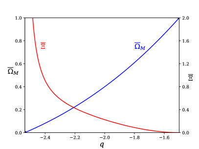
Figure 1: The stasis abundance ${\overline{\Omega}}_{M}$ (blue) and coldness ${\overline{\Xi}}$ (red), plotted as functions of $q$ within the allowed range $q_{\rm min}<q<q_{\rm max}$, with $\widehat{C}=1$. The abundance curve is plotted relative to the axis along the left edge of the frame, while the coldness is plotted relative to the axis along the right edge. We see that ${\overline{\Omega}}_{M}$ varies between $0$ and $1$ within this range, as expected, while ${\overline{\Xi}}\to\infty$ as $q\to q_{\rm min}$ and ${\overline{\Xi}}\to 0$ as $q\to q_{\rm max}$.

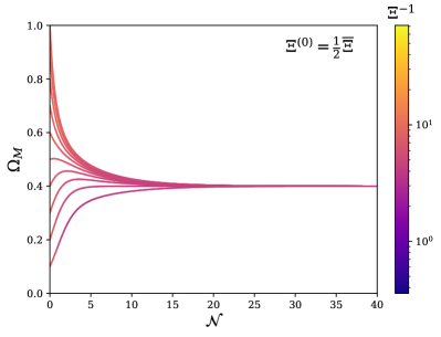
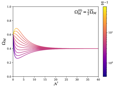
Figure 2: The matter abundance $\Omega_{M}$, plotted as a function of the number ${\cal N}$ of $e$-folds of cosmological expansion which have occurred since an early fiducial time. At each moment the color of the curve indicates the corresponding value of the coldness $\Xi$. For all plots, we have taken benchmark values $q=-2$ and $\widehat{C}=1$ and simply adjusted either the initial abundance $\Omega_{M}$ or the initial coldness $\Xi$, as shown in the figures. Indeed, both quantities eventually begin to exhibit stasis, with constant values persisting across many $e$-folds of cosmological expansion.

We thus conclude that our system necessarily evolves into an extended stasis epoch, regardless of its initial conditions pertaining to either initial matter (or radiation) abundance or initial coldness. This is therefore a direct demonstration that the stasis phenomenon can be extended into the thermal domain, with a prolonged period of stasis experienced not only by the energy abundances but also by thermodynamic quantities — such as coldness — which involve the temperature of the matter prior to annihilation.

At first glance it might seem that this is not a true thermal stasis because we have approximated ${\overline{\Omega}}_{\rm KE}\ll 1$ in deriving this non-trivial fixed-point solution. Phrased somewhat differently and more precisely, the fixed-point solution has ${\overline{\Omega}}_{\rm KE}=0$, thus suggesting that the temperature at that point is zero. However, while this is true, we must remember that in general our system does not spend the many $e$-folds of stasis (such as those shown in Fig. 1) sitting at the fixed-point solution. Instead, strictly speaking, this time is spent in approaching the fixed-point solution more and more closely. This is true for all of the stasis situations studied in the literature. Moreover, in the present case, we have not only a non-zero $\Omega_{\rm KE}$ at all points along this evolution, but also a non-zero temperature. Thus, we have a true thermal situation throughout this time period, and our pumps are operating at all points along this trajectory.

This stasis epoch can therefore be characterized as follows:

• Our annihilation pumps transfer matter to radiation and serve to counteract the tendency of the matter (radiation) abundance to increase (decrease) due to cosmological expansion. In this way, the abundances $\Omega_{M}$ and $\Omega_{\gamma}$ are kept essentially constant at non-trivial values which depend on $q$ but not on $\widehat{C}$.

• While this is happening, the actual matter energy density $\rho_{M}$ of the $\phi$-particle gas is dropping rapidly due to the combined effects of cosmological expansion and $\phi$-particle annihilation.

• Likewise, the temperature $T$ of the $\phi$-particle gas is also dropping. This occurs due to cosmological expansion [as evident from the first term on the right side of Eq. (15)], but this effect is partially mitigated by our pumps since $q<0$ [as discussed in Eq. (26)].

• Even though both $\rho_{M}$ and $T$ are dropping throughout the stasis epoch, they are dropping in such a balanced way as to hold the coldness $\Xi\equiv T^{q}\rho_{M}/m^{q+4}$ fixed at a non-trivial value which depends on both $q$ and $\widehat{C}$.

• The fact that the temperature of the $\phi$-particle gas is dropping during the stasis epoch implies that $\Omega_{\rm KE}$ is also dropping, thereby justifying setting $\Omega_{\rm KE}=0$ when deriving our non-trivial limiting fixed-point solution. Moreover, the fact that $\Omega_{\rm KE}$ quickly becomes negligible during the approach to the fixed point is responsible for the fact that we can approximate $\Omega_{\gamma}\approx 1-\Omega_{M}$ as we approach stasis along this trajectory, which is why a constant $\Omega_{M}$ implies a constant $\Omega_{\gamma}$ as well.

Given this state of affairs, it is natural to wonder how this stasis is able to persist across so many $e$-folds of cosmological expansion — a concern heightened by the fact that only a single matter species is involved. Ultimately, this feature is tied to the unique form of our pump. As we have seen, our $\phi$-particle annihilation pumps for both energy density and kinetic energy density scale as

$$P^{(\rho)}~{}\sim~{}\rho_{M}^{2}~{}~{}~{}~{}~{}\Longrightarrow~{}~{}~{}~{}~{}P~{}\sim~{}\rho_{M}\Omega_{M}~{}.$$ (35)

Indeed, we see that even our abundance-transferring pumps $P$ have a factor which scales with $\rho_{M}$ rather than with $\Omega_{M}$. However, $\rho_{M}$ is dropping to zero throughout our stasis epoch. Thus, as the energy density associated with our single matter species $\phi$ slowly disappears from our system, the corresponding pump also slowly turns off. Indeed, our pumps always operate in direct proportion to the remaining energy density. Our stasis therefore remains in balance even as we proceed further and further out along the tail of the phase-space distribution of our slowly vanishing population of $\phi$ particles. We emphasize that this feature did not appear in any previous stasis discussions in the literature since the pumps $P^{(\rho)}$ that were utilized in the previous cases were all linear in $\rho_{M}$, implying that $P\sim\Omega_{M}\sim{\rm constant}$ as far as their dependence on energy densities is concerned. We thus see that the stasis we have derived here has a very different phenomenology and operates in a fundamentally different fashion.

Of course, in writing Eq. (35) we have disregarded the temperature-dependence of our pumps. From Eq. (25) we see that

$$P_{M,\gamma}~{}\sim~{}T^{q/2}~{},~{}~{}~{}~{}~{}P_{{\rm KE},\gamma}~{}\sim~{}T^{q/2+1}~{}.$$ (36)

Thus, while $P_{M,\gamma}$ always scales inversely with $T$ as the temperature of our $\phi$-particle gas drops, we see that $P_{{\rm KE},\gamma}$ scales inversely with $T$ only for $q>-2$. Indeed, for smaller $q$ we find that both $P_{{\rm KE},\gamma}$ and the temperature $T$ drop together — an effect that lies beyond the energy-density scaling effect discussed above and which tends to further suppress the activity of this pump as our $\phi$-particle gas cools and dissipates.

VII Thermal Stasis as a Global Attractor

It is straightforward to demonstrate that the non-trivial fixed-point solutions for $({\overline{\Omega}}_{M},{\overline{\Xi}})$ in Eq. (32) are also global attractors. We have already seen evidence of this attractor behavior in Fig. 2. As a first step, we note that for a given value of $q$, we may assess whether that the corresponding fixed-point solution is a local attractor by evaluating the $2\times 2$ Jacobian matrix for our dynamical equations for $d\Omega_{M}/d{\cal N}$ and $d\Xi/d{\cal N}$ and then examining the signs of its two eigenvalues $\lambda_{\pm}$ at that fixed point. In Fig. 3, we present a parametric plot of these eigenvalues as $q$ is varied within the range $q_{\rm min}<q<q_{\rm max}$ for which our non-trivial fixed-point solution exists. These eigenvalues trace out the red solid curve. Within this $q$-range, we see that both eigenvalues lie within the yellow-shaded region wherein both $\lambda_{+}$ and $\lambda_{-}$ are negative. Thus, we may conclude that across this entire range of $q$, the non-trivial fixed-point solution within this range is indeed a local attractor.

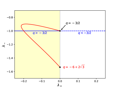
Figure 3: Parametric plot of the Jacobian eigenvalues $(\lambda_{+},\lambda_{-})$ as the parameter $q$ is varied. In all cases these eigenvalues are evaluated for a given fixed-point solution. The red curve indicates the combinations of these eigenvalues associated with the non-trivial fixed point in Eq. (32), while the blue horizontal line indicates the eigenvalues associated with the trivial fixed point described in third bullet below Eq. (34). Thus, we see that not only are ${\overline{\Omega}}_{M}$ and ${\overline{\Xi}}$ independent of $q$ for this trivial fixed point, but $\lambda_{-}$ is as well. As discussed in the text, the non-trivial fixed point is an attractor throughout the entirety of the range $-6+2\sqrt{3}\leq q\leq-3/2$, while the trivial fixed point is an attractor only for $q>-3/2$. Note that these fixed points are attractors only when both eigenvalues $\lambda_{\pm}$ are negative and hence lie within the yellow shaded region. The corresponding lines are then shown as solid rather than dashed. Interestingly, the red and blue curves intersect precisely at $q=-3/2$, where they both correspond to the solution $({\overline{\Omega}}_{M},{\overline{\Xi}})=(0,1)$. The fact that the red and blue curves intersect at only one point ensures that there is never more than one attractor solution as $q$ crosses the $q=-3/2$ boundary. Thus, as $q$ increases from $q=-6+2\sqrt{3}$, our attractor solution follows the red curve until reaching the $q=-3/2$ point and then switches to the solid blue line for $q>-3/2$.

Within Fig. 3 we have also plotted the eigenvalues associated with the trivial fixed-point solution indicated in the third bullet in the paragraph below Eq. (34). These eigenvalues fill out the blue horizontal line. When $q<q_{\rm max}=-3/2$, we see that $\lambda_{+}$ is positive, telling us that this solution is not an attractor for such values of $q$. However, as $q$ increases beyond $q_{\rm max}$, we pass across into the yellow-shaded region within which both eigenvalues are negative and within which this trivial fixed-point becomes an attractor. Interestingly, the blue line associated with our trivial fixed-point solution intersects the red curve associated with our non-trivial fixed-point solution precisely at $q=q_{\rm max}=-3/2$. Indeed, as $q$ increases through the point $q=-3/2$, our non-trivial fixed-point solution ceases to be an attractor and our trivial fixed-point solution becomes an attractor. Thus $q=-3/2$ marks a continuous boundary between these two different solutions. Indeed, even the corresponding solutions for ${\overline{\Omega}}_{M}$ and ${\overline{\Xi}}$ are continuous across this boundary.

Since the Jacobian analysis we have presented above characterizes only the local behavior of our system — i.e., its behavior within the vicinity of the fixed point — it still remains to be seen whether these fixed points are in fact global attractors toward which our system dynamically flows regardless of its initial conditions. However, within the $q$-ranges we have been discussing, it turns out that this is indeed the case. We can be verify this by examining the trajectory along which the system described in Eq. (28) dynamically evolves in the $(\Omega_{M},\Xi)$-plane, given an arbitrary initial configuration within that plane. In Fig. 5 we show a number of such trajectories for the benchmark value $q=-2$. We find that regardless of the initial location of our system within this plane, our system is inevitably drawn toward our non-trivial fixed-point solution, indicating that this fixed point is not only an attractor but also global rather than merely local.

It is also instructive to examine what happens when we choose $q$ outside the range specified in Eq. (33). The behavior of our system ultimately depends on whether $q<q_{\rm min}$ or $q>q_{\rm max}$. Both behaviors are shown in Fig. 5. In the left plot, we consider a situation with $q<q_{\rm min}$. In this case, our flow lines all tend towards small values of $\Omega_{M}$ with ever-increasing values of $\Xi$. Indeed, no fixed-point solution is ever reached. By contrast, for $q>q_{\rm max}$, all of our flow lines are pulled toward the trivial fixed point at $({\overline{\Xi}},{\overline{\Omega}}_{M})=(0,1)$, as anticipated. Thus even our trivial fixed point is a global attractor for $q>-3/2$.

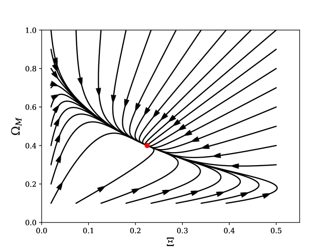
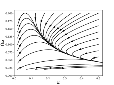
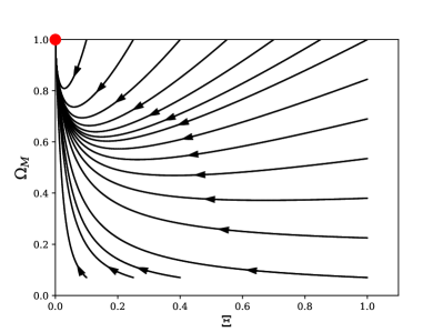
Figure 4: Attractor behavior for our thermal stasis when $q$ lies within the allowed stasis range in Eq. (33). These trajectories within the $(\Xi,\Omega_{M})$-plane correspond to the time evolution of the cosmological system described in Eq. (28), with chosen benchmark values $q=-2$ and $\widehat{C}=1$. The central red dot towards which all flow lines tend is our corresponding stasis solution with $({\overline{\Xi}},{\overline{\Omega}}_{M})=(9/40,2/5)$. We note that this plot was made assuming a relatively small initial value for $\Omega_{\rm KE}$, but similar plots arise regardless of the initial value of $\Omega_{\rm KE}$.

Figure 5: Time evolution of our cosmology when $q$ is outside the stasis range $q_{\rm min}<q<q_{\rm max}$ in Eq. (33), with either $q<q_{\rm min}$ (left panel) or $q>q_{\rm max}$ (right panel). The left and right panels shown correspond to the benchmark values $q=-2.7$ and $q=-1.3$ respectively, with $\widehat{C}=1$. Note that $\Xi$ can either increase or decrease if $q<q_{\rm max}$, but can only decrease if $q>q_{\rm max}$. For $q<q_{\rm min}$, our system has no fixed point, and all of the flows proceed toward small $\Omega_{M}$ but ever-increasing coldness $\Xi$. By contrast, for $q>q_{\rm max}$, our system is attracted to the trivial fixed point at $({\overline{\Xi}},{\overline{\Omega}}_{M})=(0,1)$.

VIII A Particle-Physics Mechanism for Achieving Thermal Stasis

In the previous section, we demonstrated that an extended epoch of matter/radiation stasis can emerge in a thermal context, and with only a single matter species $\phi$, provided not only that this species annihilate into radiation via a $2\to 2$ process of the form $\phi\phi\to\chi\chi$, but also that the thermally averaged cross-section for this annihilation process take the form given in Eq. (16) with $q$ within the range in Eq. (33).  In this section, we outline how these conditions can be realized in a particle-physics context.

As one might imagine, the principal challenge in constructing a particle-physics model of thermal stasis along these lines is to ensure that the swept-volume rate $\sigma v$ for matter-particle annihilation takes the form in Eq. (16) with a value of $q$ within the desired range in Eq. (33). Indeed, as we shall discuss below, typical particle-physics models that one can construct along these lines lead to values of $q$ which are either above or below this range. Such models therefore do not yield a stasis epoch. However, as we shall now demonstrate, there do exist particle-physics mechanisms which lead to suitable values of $q$. In what follows, we describe one such mechanism — one which leads specifically to a value $q=-2$ for this parameter. This mechanism rests on fundamental ideas in quantum field theory and can be realized within a broad variety of particle-physics contexts. We shall therefore keep the following discussion as model-independent as possible.

We focus on the case in which the annihilation process $\phi\phi\to\chi\chi$ proceeds primarily through an $s$-channel mediator $X$, as illustrated in Fig. 6. For concreteness, we take $\phi$, $\chi$, and $X$ all to be scalar fields in what follows, though we note that this mechanism can be realized for certain other combinations of spin assignments as well. We shall let $m_{X}$ denote the mass of $X$ and continue to let $m$ denote the mass of $\phi$.  In the CM frame, the incoming $\phi$ particles have the four-momenta

$$p_{1}~{} = ~{}(E,\vec{p}_{\rm CM})$$

$$p_{2}~{} = ~{}(E,-\vec{p}_{\rm CM})$$ (37)

where $\pm\vec{p}_{\rm CM}$ are the three-momenta of our incoming particles as seen in the CM frame and where we assume that each of these incoming particles is on shell. Thus, for an $s$-channnel propagator in the CM frame, the total four-momentum flowing through the $X$ particle is

$$p_{X}~{}\equiv~{}p_{1}+p_{2}~{}=~{}(2E,\vec{0})~{},$$ (38)

from which we deduce that

$$p_{X}^{2}~{}=~{}4E^{2}~{}=~{}4\left(|\vec{p}_{\rm CM}|^{2}+m^{2}\right)~{}.$$ (39)

The tree-level propagator is then given by

$$\Delta(p_{X})~{} \sim ~{}\frac{i}{p_{X}^{2}-m_{X}^{2}}$$ (40)

$$= ~{}\frac{i}{4(|\vec{p}_{\rm CM}|^{2}+m^{2})-m_{X}^{2}}$$

$$= ~{}\frac{i}{4|\vec{p}_{\rm CM}|^{2}-\mu^{2}}~{},$$

where

$$\mu^{2}~{}\equiv~{}m_{X}^{2}-4m^{2}~{}.$$ (41)

It should be noted that we are not assuming that $m_{X}=2m$ (for which we would have $\mu=0$), and thus $\mu$ appears as a new free parameter. In general, we see from Eq. (41) that $\mu^{2}$ can have either sign.

Figure 6: Feynman diagram for the $s$-channel annihilation process through which two $\phi$ particles annihilate into radiation through a mediator $X$, complete with a one-loop radiative correction for $m_{X}$.  Here the $\phi$ particles constitute the matter in our model and are indicated in blue, while the resulting radiation is indicated in green and the mediator particle $X$ is indicated in red. The one-loop correction for the propagator (shown in gray) comprises loops of matter or radiation.

If $|\mu^{2}|\ll 4|\vec{p}_{\rm CM}|^{2}$, then $\Delta\sim 1/|\vec{p}_{\rm CM}|^{2}$, which leads to $q=-4$. By contrast, if $|\mu^{2}|\gg 4|\vec{p}_{\rm CM}|^{2}$, we find that $\Delta$ becomes independent of $|\vec{p}_{\rm CM}|$ and thus $q=0$. In all other cases, $q$ will vary between $-4$ and $0$. However, we will never have a non-zero range of $|\vec{p}_{\rm CM}|$ values for which $q$ is effectively constant and lies within the desired stasis range $-6+2\sqrt{3}<q<-3/2$.

We now investigate what happens when we include the one-loop radiative correction to the $X$ propagator. In particular, we shall let $\Pi_{X}(p_{X}^{2})$ denote the one-loop contribution to the self-energy of the mediator, which corresponds to the one-particle irreducible (1PI) “bubble” within the $X$ propagator in Fig. 6. Our propagator will then take the form

$$\Delta(p_{X})~{}\sim~{}\frac{i}{p_{X}^{2}-m_{X}^{2}+\Pi_{X}(p_{X}^{2})}~{}.$$ (42)

Despite the fact that $\Pi_{X}(p_{X}^{2})$ is a one-loop radiative correction, we shall find this term can nevertheless become dominant if we are near a resonance in the propagator.

The mediator self-energy $\Pi_{X}(p_{X}^{2})$ depends on the specific model under study and is in general a complex-valued function. Since the real part of $\Pi_{X}(p_{X}^{2})$ can be absorbed by a redefinition of $m_{X}$, the $X$-propagator may be written in the form

$$\Delta(p_{X})~{}\sim~{}\frac{i}{p_{X}^{2}-m_{X}^{2}+im_{X}\widetilde{\Gamma}_{X}(p_{X}^{2})}~{},$$ (43)

where we have defined

$$\widetilde{\Gamma}_{X}(p_{X}^{2})~{}\equiv~{}\frac{1}{m_{X}}\textrm{Im}\,\Pi_{X}(p_{X}^{2})~{}.$$ (44)

In what follows, we shall refer to this quantity as the “off-shell width” of the mediator. Despite this choice of terminology, however, we emphasize that $\widetilde{\Gamma}_{X}(p_{X}^{2})$ is in general a non-trivial function of $p_{X}^{2}$, and is not in general equal to the proper decay width of $X$.

For any model which gives rise to an $s$-channel annihilation diagram of the form depicted in Fig. 6, $\widetilde{\Gamma}(p_{X}^{2})$ receives contributions from two processes: one with a pair of $\chi$ particles running in the loop and one with a pair of $\phi$ particles running in the loop. We shall denote these contributions $\widetilde{\Gamma}_{X\to\chi\chi}(p_{X}^{2})$ and $\widetilde{\Gamma}_{X\to\phi\phi}(p_{X}^{2})$, respectively. Thus, in general, we have

$$\widetilde{\Gamma}_{X}~{}=~{}\widetilde{\Gamma}_{X\to\chi\chi}+\widetilde{\Gamma}_{X\to\phi\phi}~{}.$$ (45)

Since our regime of interest for stasis is that in which our population of $\phi$ particles is highly non-relativistic, we are particularly interested in how $\widetilde{\Gamma}_{X}(p_{X}^{2})$ behaves as a function of $|\vec{p}_{\rm CM}|$ when $|\vec{p}_{\rm CM}|$ is small. Within this regime, we may obtain a reliable approximation for $\widetilde{\Gamma}_{X}(p_{X}^{2})$ by expanding this function as a Taylor series in $|\vec{p}_{\rm CM}|$ around $|\vec{p}_{\rm CM}|=0$ and retaining only the leading terms. With only minor assumptions about the model, it can be shown that the $|\vec{p}_{\rm CM}|$-independent term and the term linear in $|\vec{p}_{\rm CM}|$ are both necessarily non-zero. Thus, within our regime of interest, $\widetilde{\Gamma}_{X}$ is well approximated by an expression of the form

$$\widetilde{\Gamma}_{X}~{}\approx~{}c_{0}+c_{1}|\vec{p}_{{\rm CM}}|~{}$$ (46)

where $c_{0}$ and $c_{1}$ are arbitrary non-zero, model-dependent constants.

Substituting this expression into Eq. (43), we obtain

$$\Delta(p_{X})~{} \sim ~{}\frac{i}{4|\vec{p}_{\rm CM}|^{2}-\mu^{2}+im_{X}\left(c_{0}+c_{1}|\vec{p}_{\rm CM}|\right)}$$

$$= ~{}\frac{i}{m^{2}}\left[\widetilde{\alpha}+i\beta\frac{|\vec{p}_{{\rm CM}}|}{m}+4\frac{|\vec{p}_{{\rm CM}}|^{2}}{m^{2}}\,\right]^{-1}~{}~{}~{}~{}~{}~{}$$

$$= ~{}\frac{i}{\alpha m^{2}}\,\frac{1}{e^{i\theta}+ixy+x^{2}}~{},$$ (47)

where in passing from the second to the third line we have defined

$$\widetilde{\alpha}~{}=~{}-\frac{\mu^{2}}{m^{2}}+\frac{ic_{0}m_{X}}{m^{2}}~{},~{}~{}~{}~{}\beta~{}=~{}c_{1}\frac{m_{X}}{m}~{},$$ (48)

and where in passing from the third to the fourth line we have expressed the complex coefficient $\widetilde{\alpha}$ in terms of its modulus $\alpha$ and complex phase $\theta$, whence

$$x~{}=~{}\sqrt{\frac{4}{\alpha}}\,\frac{|\vec{p}_{{\rm CM}}|}{m}~{},~{}~{}~{}~{}y~{}=~{}\frac{\beta}{\sqrt{4\alpha}}~{}.$$ (49)

Our original question was to determine the circumstances under which the propagator $\Delta$ might scale as $|p_{\rm CM}|^{-1}$, since this would lead to amplitudes with the desired scaling with $q=-2$. Given the above results, we are now in a position to answer this question. Defining $f(x)\equiv 1/|e^{i\theta}+ixy+x^{2}|$, we find

• $f(x)\sim{\rm constant}$ for $x\ll 1/y$;

• $f(x)\sim 1/x$ for $1/y\ll x\ll y$; and

• $f(x)\sim 1/x^{2}$ for $x\gg y$.

Indeed, these results hold for all $y$ and all $\theta$. We thus see that we can indeed achieve the desired inverse linear scaling for our propagator across a significant interval of momenta $|\vec{p}_{\rm CM}|$ so long as

$$y~{}\gg~{}1~{},~{}~{}~{}~{}1/y~{}\ll~{}x~{}\ll~{}y~{}.$$ (50)

However, as discussed previously, we also know that our incoming $\phi$ particles must be non-relativistic (so that they can be interpreted as matter rather than radiation). This then implies the additional constraint

$$x~{}\ll~{}\sqrt{4/\alpha}~{}.$$ (51)

The cosmological implications of the criterion in Eq. (50) for stasis in can be understood as follows. Let us assume, as we did in Sect. II, that additional scattering processes in the theory serve to maintain kinetic equilibrium among the population of $\phi$ particles, and that this population of particles can be characterized by a temperature $T$. At values of $T$ for which the phase-space integrals in $\langle\sigma v\rangle$ and $\langle({\rm KE}_{a}+{\rm KE}_{b})\sigma v\rangle$ are each dominated by the contribution from particles with $|\vec{p}_{\rm CM}|$ within the range specified in Eq. (53), these thermal averages are well approximated by the expressions in Eq. (24) with $q=-2$. Thus, at such temperatures, the universe evolves toward stasis. By contrast, at values of $T$ for which these phase-space integrals receive sizable contributions from particles with $|\vec{p}_{\rm CM}|$ outside this range, $\langle\sigma v\rangle$ and $\langle({\rm KE}_{a}+{\rm KE}_{b})\sigma v\rangle$ do not exhibit the appropriate scaling behavior with $T$ and the system does not evolve toward stasis.

In order to obtain an estimate of the range of $T$ within which our system is indeed attracted toward stasis, we can associate a given value of $T$ with a “typical” value of $|\vec{p}_{\rm CM}|$ — i.e., a value near the peak in the Maxwell-Boltzmann distribution — via the relation

$$T~{}\sim~{}|\vec{p}_{{\rm CM}}|^{2}/m~{},$$ (52)

where in making this identification we have disregarded ${\cal O}(1)$ factors. Since the constraint in Eq. (50), expressed in in terms of $|\vec{p}_{\rm CM}|$, is

$$\frac{\alpha}{\beta}m~{}\ll~{}|\vec{p}_{\rm CM}|~{}\ll~{}\frac{\beta}{4}m~{},$$ (53)

it therefore follows that the temperature window wherein the stasis attractor is the solution to the coupled evolution equations in Eq. (9) is

$$T_{\rm min}~{}\lower 3.01385pt\hbox{{\mbox{$\;\stackrel{{\scriptstyle\textstyle<}}{{\sim}}\;$}}}~{}T~{}\lower 3.01385pt\hbox{{\mbox{$\;\stackrel{{\scriptstyle\textstyle<}}{{\sim}}\;$}}}~{}T_{\rm max}~{},$$ (54)

where we have defined

$$T_{\rm max}~{} \equiv ~{}\frac{\alpha^{2}}{\beta^{2}}m$$

$$T_{\rm min}~{} \equiv ~{}\frac{\beta^{2}}{16}m~{}.$$ (55)

As long as $T$ remains within the rough window in Eq. (54), the universe continues to evolve toward stasis. However, as time goes on and the temperature of the $\phi$-particle gas decreases, eventually $T$ drops below $T_{\rm min}$ and the stasis attractor ceases to be the solution to the coupled evolution equations in Eq. (9). Indeed, when $T$ falls below this threshold, $\langle\sigma v\rangle$ no longer increases as the kinetic-energy density of the $\phi$ particles decreases. As a result, $\phi\phi\to\chi\chi$ annihilation becomes inefficient and $\Omega_{M}$ increases until the rest-mass-energy density of the $\phi$-particle gas dominates the total energy density of the universe. This, then, is the manner in which stasis naturally ends in models which make use of this mechanism, with the universe subsequently becoming dominated by massive matter.

IX Conclusions and Directions for Future Research

In all of its realizations, cosmological stasis is ultimately a consequence of processes which transfer energy density from one cosmological component to another in a way which counteracts the effects of Hubble expansion. A variety of processes, including particle decay Dienes et al. (2022a, 2023), Hawking radiation Barrow et al. (1991); Dienes et al. (2022b), and the overdamped/underdamped transition of homogeneous scalar-field zero-modes Dienes et al. (2024) give rise to pumps which can accomplish this feat. However, the pump rate associated with each of these processes depends only on the intrinsic properties (e.g., masses or decay widths) of individual objects — individual particles, black holes, etc. — within the system, or on the dynamical variables $\Omega_{i}$ and $H$, or on $t$ itself. In other words, the pump rate was independent of the external environment in which these constituent objects found themselves.

In this paper, by contrast, we have demonstrated that a pump with the properties appropriate for stasis can also arise from a wholly different class of physical process — processes in which this rate depends on additional dynamical variables which characterize the extrinsic properties of a cosmological population of particles, black holes, or other individual objects. In other words, in such cases, the pump rates depend not only on the intrinsic properties of these constituent objects, but also on their external cosmological environment. We have shown, for example, that the annihilation of a gas consisting of a single species of non-relativistic matter particle into radiation — a process whose rate depends not only on the overall abundance $\Omega_{M}$ of these matter particles, but also on their temperature $T$ — can, under the certain conditions, give rise to such a pump. Notably, unlike in all realizations of stasis which have previously been identified in the literature, stasis emerges in this context in a manner which does not require a tower of states. Moreover, we have shown that stasis nevertheless emerges as a dynamical attractor in systems wherein these conditions are satisfied.

The principal such condition is that the swept-volume rate $\sigma v$ for the annihilation process must scale in an appropriate manner with the momenta of the annihilating matter particles in the CM frame. While this condition is a non-trivial one, we have detailed a particle-physics mechanism through which such a momentum-dependence can be achieved.

Several additional comments are in order. First, as we have already noted, thermal stasis — unlike its non-thermal cousins — involves thermal effects in an intrinsic way, i.e., as part of the pump that establishes and sustains the resulting stasis. That said, we find it remarkable that this stasis does not simply keep the temperature of our $\phi$-particle gas constant, as might naively been anticipated. Such a result, of course, would have rendered a thermal realization of stasis challenging to realize in an expanding universe, since additional dynamics would be required in order to maintain this temperature at a constant value in such a context. However, what we find is that our thermal stasis also has a continually dropping temperature! That said, the rate at which the temperature drops is modified during thermal stasis, due to the manner in which annihilation affects different parts of the phase-space distribution of the $\phi$ particles. In particular, the universe cools slightly more slowly than one would expect as a result of expansion alone. Indeed, what we have a discovered is that there is an entirely new thermodynamic quantity, the coldness $\Xi$, which remains fixed during stasis. This observation also suggests that it is coldness, rather than temperature, which may be a more fundamental dynamical variable as far as stasis is concerned.

Second, despite the absence of a tower of states, the realization of thermal stasis that we have described in Sect. VIII comes with its own graceful exit. In tower-based realizations of stasis, the stasis epoch stretches across a time interval during which the action of the pump incrementally proceeds towards the lower portions of the tower Dienes et al. (2022a, 2023, 2024). The exit from the stasis epoch then arises once we reach the bottom of the tower. As a result, once stasis ends, the universe subsequently becomes dominated by that cosmological component which participates in the stasis dynamics and which has the highest equation-of-state parameter. For thermal stasis, by contrast, there is no tower. We nevertheless continue to have an extended stasis epoch, and this in turn ends through a different mechanism: once the temperature of our $\phi$-particle gas eventually drops below the temperature $T_{\rm min}$ in Eq. (55), $\langle\sigma v\rangle$ no longer increases as the kinetic-energy density of the $\phi$ particles decreases. As a result, $\phi\phi\to\chi\chi$ annihilation becomes inefficient and $\Omega_{M}$ increases until the $\phi$-particle gas (i.e., the component with the lowest equation-of-state parameter) ultimately comes to dominate the energy density of the universe. Thus, in this scenario, stasis ends not with a bang, but with a WIMP-er. Clearly the graceful exits for thermal and tower-based realizations of stasis are qualitatively quite different. We nevertheless see that each of our stasis epochs comes with its own intrinsic exit.

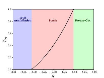
Figure 7: The stasis abundance ${\overline{\Omega}}_{M}$, plotted as a function of $q$ within the range $-6+2\sqrt{3}<q<-3/2$ (pink background) for which thermal stasis can be achieved. For $q<-6+2\sqrt{3}$ (blue background), the swept-volume rate $\sigma v$ remains sufficiently high for arbitrarily small $|\vec{p}_{\rm CM}|$ — and thus at arbitrarily large distance scales — that the population of $\phi$ particles annihilates completely. By contrast, for $q>-3/2$ (green region), this swept-volume rate becomes sufficiently small for small $|\vec{p}_{\rm CM}|$ that $\phi$ particles cannot find each other at late times and therefore effectively freeze out. Thermal stasis may thus be interpreted as a phenomenon which interpolates between these two regimes, with a swept-volume rate that decreases sufficiently rapidly with increasing $|\vec{p}_{\rm CM}|$ that total annihilation is avoided, and yet not so rapidly that a relic population of $\phi$ particles freezes out at low temperatures.

On a final note, we observe that the manner in which ${\overline{\Omega}}_{M}$ varies with $q$ across the range specified in Eq. (33) suggests that this stasis window can be viewed as interpolating between a regime wherein our population of $\phi$ particles annihilates completely and a regime wherein this population of particles effectively freezes out. It is straightforward to understand why this is the case. In Fig. 7, we have schematically indicated a range of $q$-values that not only includes the window $-6+2\sqrt{3}<q<-3/2$ in which stasis emerges (shaded in pink), but also extends beyond this window in each direction (blue and green). We can then discuss what happens within each region in turn.

For values of $q$ below this stasis window (i.e., within the blue-shaded region), the swept-volume rate $\sigma v$ remains sufficiently high for arbitrarily small $|\vec{p}_{\rm CM}|$ — and thus at arbitrarily large distance scales — that the population of $\phi$ particles annihilates completely. As a result, there is no stasis in the blue-shaded region: the pump is overwhelmingly effective for such values of $q$, and $\Omega_{M}$ simply falls to zero.

At the opposite extreme, for values of $q$ above the stasis window (i.e., within the green-shaded region), $\sigma v$ becomes sufficiently small for small $|\vec{p}_{\rm CM}|$ that $\phi$ particles cannot find each other at late times. A situation then develops which is in many ways similar to the situation that arises when a WIMP freezes out. While there are of course salient differences between the freeze-out mechanics of a WIMP and the freeze-out mechanics of our $\phi$-particle gas — for example, the $\phi$ particles are never in thermal equilibrium with the radiation particles into which they annihilate — the qualitative result is the same: a relic population of $\phi$ particles is left over once these particles effectively cease annihilating with each other, and this population of $\phi$ particles comes to dominate the energy density of the universe at late times, with $\Omega_{M}$ becoming effectively unity. Thus once again no stasis is possible. Indeed, we note that this phenomenon is precisely how the graceful exit from stasis discussed earlier comes to pass: below $T_{\rm min}$, the value of $q$ is effectively no longer $q=-2$ but instead $q=0$, and thus our population of matter particles freezes out.

Finally, between these two extremes lies our stasis window (shaded in pink). For $q$ within this window, $\sigma v$ decreases with increasing $|\vec{p}_{\rm CM}|$ sufficiently rapidly that total annihilation is avoided, but not so rapidly that a relic population of $\phi$ particles freezes out at low temperatures. Thus a bona fide stasis emerges, with corresponding values of ${\overline{\Omega}}_{M}$ that interpolate between the two extremes, as illustrated in Fig. 7. It is noteworthy — and even somewhat remarkable — that this transition between the two extremes outlined above does not occur abruptly at some critical value of $q$, but rather over a non-zero range of $q$-values, with stasis emerging for all values of $q$ within this window and with the corresponding stasis abundance of the $\phi$-particle gas varying smoothly over the entire allowed range $0\leq{\overline{\Omega}}_{M}\leq 1$ as we traverse this window. Indeed, we see that the balancing inherent in stasis can be achieved for any $q$-value within the stasis window, with the resulting stasis abundance ${\overline{\Omega}}_{M}$ varying with the specific value of $q$.

Given our results, many avenues are now open for future research. For example, in Sect. VIII we have developed a particle-physics mechanism for achieving a swept-volume rate of the form in Eq. (17) with $q=-2$. However, it nevertheless remains to construct a concrete particle-physics model in which this mechanism is realized in a self-consistent way. Of course, any concrete model along these lines must not only yield the desired momentum-dependence for $\sigma v$ across a significant range of $|\vec{p}_{\rm CM}|$-values, but must also satisfy a number of additional self-consistency conditions and observational constraints. First steps toward the construction of such a model can be found in Ref. Barber et al. (2024).  It will also be interesting to determine the specific observational signatures to which a thermal stasis epoch might lead. Work in all of these directions is underway.