Variational Mode-Driven Graph Convolutional Network for Spatiotemporal Traffic Forecasting

Abstract

This paper focuses on spatio-temporal (ST) traffic prediction traffic using graph neural networks. Given that ST data consists of non-stationary and complex time events, interpreting and predicting such trends is comparatively complicated. Representation of ST data in modes helps us infer behavior and assess the impact of noise on prediction applications. We propose a framework that decomposes ST data into modes using the variational mode decomposition (VMD) method, which is then fed into the neural network for forecasting future states. This hybrid approach is known as a variational mode graph convolutional network (VMGCN). Instead of exhaustively searching for the number of modes, they are determined using the reconstruction loss from the real-time application data. We also study the significance of each mode and the impact of bandwidth constraints on different horizon predictions in traffic flow data. We evaluate the performance of our proposed network on the LargeST dataset for both short and long-term predictions. Our framework yields better results compared to state-of-the-art methods.

I Introduction

Traffic Management Systems (TMS) play a vital role in the growth of urbanization. The increasing number of vehicles on the road consistently pressures traffic planning and management. An Intelligent Transportation System (ITS) enhances the efficiency, reliability, and safety of transportation systems [1]. Accurate predictions help avoid congestion and improve traffic infrastructure, mitigating issues like air pollution, fuel and time wastage, and accidents. These problems directly impacts on the human health, daily life, social life, and psychological states, including lack of control, fatigue, time pressure, and stress. For effective online monitoring and prediction, smart cameras or sensors must be installed at crowded intersections, and path-planning user applications should guide individuals away from traffic jams. The traffic counts or flow holds statistical significance in data analytics, allowing predictions of increasing vehicle numbers over time and planning for traffic infrastructure accordingly. Socioeconomic indicators and policies also play roles in traffic management. The policies based on speed or flow can be implemented to prevent road crashes, motivating us to address the problem of developing accurate and robust traffic prediction methods. In this paper, we are addressing traffic prediction using a deep learning method.

I-A Related Work

In traffic forecasting, both parametric and non-parametric models are fundamental approaches for predicting future states. The choice of model depends on the size and complexity of the data, as well as the available computational resources. Parametric models include time series analysis, parametric regression, and Kalman filter models. Time series analysis models, such as the auto-regressive integrated moving average (ARIMA), seasonal ARIMA (SARIMA), and exponential smoothing. The non-parametric approaches including K-nearest neighbors, decision trees, and Support Vector machines (SVM) have been widely used.

The Box-Jenkins ARIMA model, which transforms non-stationary data to stationary data using the differences in the time series, is frequently incorporated in traffic volume prediction [2]. Another approach for prediction in [3], uses measured state data to forecast traffic flow, minimizing prediction errors based on the assumption of data stationarity (Kalman filtering theory). These parametric methods are interpretable but struggle to model complex and non-stationary traffic data effectively. Non-parametric models utilize distance metrics to determine the nearest neighbor of the current state to the historical observation in feature space [4]. These methods are rich in data requirements, less interpretable, and computationally complex. Both parametric and non-parametric methods utilize historical observed data but do not incorporate spatial information.

Due to recent advancements in deep learning, significant improvements have been made in traffic forecasting applications. The state-of-the-art methods in traffic prediction consider various factors such as spatial topology construction, spatial dependency, temporal dependency, and external factors. These advanced methods are designed to better handle the complexities of modern traffic data and provide more accurate predictions over both short (refer to horizons of up to one hour) and long term (beyond one hour) [5].

Spatial topology construction

The non-Euclidean geodesic information of the sensor network is incorporated in the model using graph neural networks (GNNs). If the graph topology is defined based on the distance between the nodes, this representation is known as a static graph. In an adaptive graph, the structure of the graph is constructed based on the temporal evolution of the data. For spatial graph modeling from the dynamic feature, [6], [7], [8] determines a self-adaptive adjacency matrix using node embeddings end-to-end learning mechanism. Dynamic graph convolutional recurrent network [9] incorporates the weighted combination of both static and dynamic graph convolution. The semantic adjacency matrix is computed using dynamic time warping distance by incorporating the time series of nodes [10]. The binary adjacency matrix represents the presence of the connection between nodes [11]. The road network is also included in distance-based graph structure [12].

Spatial dependency

To extract the spatial feature of traffic flows from the road network matrix, trafficGAN [13] implements deformable convolution [14]. Deformable convolution is used to model geometric variations. To capture the spatial dependency, mostly CNN [15], [16] and GNN  [12], [17], [7] are employed in prediction applications. The self-attention mechanism [18] is also used in the modeling of spatial dependency. In the most recent literature on traffic prediction [19], [11], the combination of attention and GNN is also encouraged to determine the spatial correlation. The meta-graph attention which is based on graph attention (GAT) is applied to determine the spatial correlations from traffic data  [20]. Chebyshev spectral convolution (ChebNet) is incorporated to learn spatial dependencies for spectral graph convolution [21]. To overcome the smoothing issues in GNNs in deeper networks that impact the long-range dependencies, the spatial-temporal graph ordinary differential equation (STGODE) block is proposed in [10]. STGODE captures the spatial and temporal dynamic correlations based on ODE.

Temporal dependency

Traffic prediction involves time series data used to capture sequential relationships. RNN and their optimized variants, such as LSTM and GRU, are commonly employed. These models are capable of capturing the long-range temporal dependencies [9]. However, combining of dynamic graphs with RNNs make the model computational expensive due to a large number of trainable parameters. Temporal convolution filters are also used to extract the temporal information from the data. The attention mechanism [22] in the spatio-temporal (ST) block is commonly used in predictive models [11], [19]. A combination of RNNs along with the attention mechanism is also employed. GRUs handle the short-term dependencies, while the self-attention mechanism models the long-term dependencies [8]. Three different types of attention– temporal, spatial, and channel– are applied to capture spatio-temproal correlations [18]. However, this proposed mechanism increases the computational, time complexity, and number of parameters compared to CNNs. CNNs and TCNs have proven more efficient in capturing complex spatio-temporal relationships. The transformer encoder-decoder architecture is implemented for the temporal pattern in [17], [20]. Typically, the encoder is implemented to learn historical traffic information and the decoder is incorporated to make predictions.

External factors

Traffic data consists of complex dynamics that depend on various factors socio-economic, land uses land covers, population density, road capacity, and cultural or public events. To apply self-attention to the point of interest (POI) of each region, POI-MetaBlock is included in deep neural network (DNN) [23]. To effectively capture temporal correlation, the external weather data is incorporated in DNNs for traffic flow forecasting in [24]. The non-traffic data such as rainfall [25] is also included in the model. Information such as holidays, weather, and nearby POIs are served as the input to the Large Language Models (LLMs) [26]. These factors serve as the features of DNNs that assist the network in extracting the spatial and temporal correlation from the traffic data.

Fourier domain analysis is also used in traffic forecasting, where the traffic data is segregated into frequency components. However, the limitation of the Fourier Transform is assumed that the data should be stationary. So, many signal processing-based methods have been introduced for the decoupling of signals. Various methods are commonly used for signal decomposition, including the well-known methods Empirical Mode Decomposition (EMD) [27], Ensemble EMD (EEMD) [28], Complete Ensemble EMD with Adaptive Noise (CEEMDAN) [29], Multivariate EMD (MEMD) [30], and Variational Mode Decomposition (VMD) [31]. The traffic data is decomposed into periodic, residual, and volatile components using the EMD method. A Bi-directional LSTM model is incorporated to model the volatile component [32]. A hybrid model, combining Improved CCEMDAN (ICCEMDAN) and GRU, is proposed to predict the parking demand [33]. Short-term traffic flow is predicted using VMD and LSTM [34]. The encoder-decoder architecture is incorporated for feature extraction from mode functions decomposed by VMD in short-term traffic flow prediction [35].

I-B Contribution

The state-of-the-art methods focus on short-term prediction using the decomposition methods. The impact assessment of noise and the effectiveness of each mode need to be considered in the prediction analysis using DNNs. In this work, we study both short-term and long-term prediction using a hybrid model (VMD + ASTGCN) approach. The main contributions of this work are summarized below,

• In our hybrid framework for spatio-temporal forecasting, we propose to decompose the spatio-temporal traffic data into modes representing the granularity of the data using VMD. The spatial and temporal attention are applied to the decomposed features, followed by Cheby-Net graph convolution and time convolution to predict the future states over the long term.

• We conduct an in-depth analysis of our proposed architecture, and formulate a method to determine the best-fit value of the number of modes in the real-time dataset. Additionally, we highlight the impact assessment of different hyper-parameters on the long-term prediction performance of the model.

• We evaluate the performance of the proposed architecture on the LargeST[36] dataset across three different regions using three metrics mean absolute error (MAE), root mean square error (RMSE), and mean average percentage error (MAPE). The collective nodes of the LargeST dataset are $6902$, sampled at $15$ minute time interval over one year (containing $241$ million spatio-temporal observations). As an illustration, Fig. 1 demonstrates the prediction loss of our proposed model on the SD region.

The rest of the paper is organized as follows. Section II describes the adopted notation and formulates the problem statement. Section III presents the detailed architecture of the network used in our framework along with the mathematical formulation of the decomposition method. Section IV presents the experimental analysis and the improvements enabled by our methods before Section V concludes the paper.

[controls,loop,autoplay,width=]1figures/sd_horizon_3/frame_010

(a)

[controls,loop,autoplay,width=]1figures/sd_horizon_6/frame_010

(b)

[controls,loop,autoplay,width=]1figures/sd_horizon_12/frame_010

(c)

Figure 1: This figure contains the visualization that shows the temporal normalized loss variations on SD region for (a) Horizon 3 (b) Horizon 6 (c) Horizon 12. (For proper visualization of animation, please open this document in Adobe Reader).

II Preliminaries

II-A Road Network

In graph theory, a road is modeled by considering different nodes at distinct joints, vertices, or intersections. Each node of the road is connected to another segment or node. The interconnectivity and distance among nodes are incorporated in a graph referred to as a road network, defined as $\mathcal{G}=(V,E,A)$, where $V$ is a set of entities or nodes, $E$ represents the connection between these entities, and $A\in\mathbb{R}^{N\times N}$ is the weighted adjacency matrix. Here, $N$ represents the total number of nodes in a traffic prediction application, which could be either the number of sensors or vertices of a road network.

II-B Temporal Traffic Network Graph

Traffic flow, the number of vehicles per unit of time in a road segment, is a key measure of traffic congestion, which also depends on the width or number of road lanes. A temporal dynamic graph is an arrangement of graph snapshots [$\mathcal{G}^{(1)},\mathcal{G}^{(2)},\dots,\mathcal{G}^{(T_{w})}$] where $\mathcal{G}^{(t)}=(V^{(t)},A^{(t)},X^{(t)})$ includes vertices $V^{(t)}$, an adjacency matrix $A^{(t)}$, and a feature matrix $X^{(t)}$ [37]. Here, $T_{w}$ is the time window depending on the horizon of the signal. The feature matrix $X^{(t)}$ may include traffic information and road network characteristics. This structure, known as the temporal traffic network graph (TTNG), explains the traffic flow among different nodes from time $[1,T_{w}]$. As an illustration, Fig. 2 depicts the sequence of temporal graphs for a traffic network.

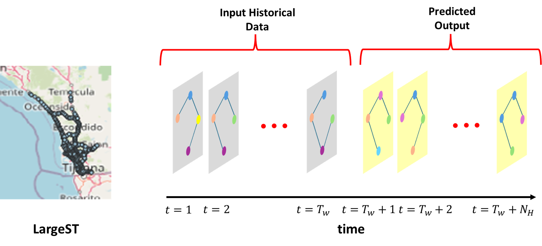
Figure 2: Left side illustrates the spatial distribution of nodes in the San Diego region, as represented in the LargeST dataset. On the right side, the TTNG structure is depicted, where the historical and current input graphs are sampled at time intervals $t=\{1,2,\dots,T_{w}\}$. The output graphs are then predicted for $t=\{T_{w}+1,T_{w}+2,\dots,T_{w}+N_{H}\}$.

II-C Problem Formulation

The dynamic evolving graph can be defined as time-dependent $\mathcal{G}^{(t)}=(V^{(t)},A^{(t)},X^{(t)})$. We assume that the vertices are constant but the features are time-dependent and are also influenced by unforeseen conditions such as road accidents, road closures, and public events, which alter the course of traffic flow. In this work, we aim to predict the future horizon traffic flow [$\boldsymbol{X}^{(T_{w}+1)},\boldsymbol{X}^{(T_{w}+2)},\dots,\boldsymbol{X}^{(T_{w}+N_{H})}$] for the next prediction horizon length $N_{H}$ given $\mathcal{G}^{(t)}$ for $t\in[1,T]$, i.e.,

$$\begin{split}[\mathcal{G}^{(1)},\dots,\mathcal{G}^{(T_{w})}]\stackrel{{\scriptstyle F}}{{\rightarrow}}[\boldsymbol{X}^{(T_{w}+1)},\dots,\boldsymbol{X}^{(T_{w}+N_{H})}],\end{split}$$

where $T$ is the length of the signal and $F$ is a deep-learning-based function that takes current and historical TTNG as input to yield the future TTNG.

III Methodology

III-A Mathematical Formulation

The mathematical formulation of the proposed framework is divided into two main steps. The first step focuses on the pre-processing of the time signal using variational mode decomposition (VMD) [31]. The second step involves the deep-learning model for spatio-temporal forecasting [11].

III-A1 Variational Mode Decomposition (VMD)

The objective of VMD is to decouple the original signal into sub-signals $u_{k}$, known as modes. The analytic signal $f_{A}(t)$ is a complex-valued function that contains only non-negative frequency components. An oscillatory signal is a valid intrinsic mode function (IMF) if it fulfills the two main conditions; the number of local extrema (minima and maxima) and zero-crossings that differ at most by one; the average value of the mode is zero [27]. The analytic signal is a complex signal where the real part comprises the original signal $f(t)$ and the imaginary part is the Hilbert transform $\mathcal{H}f(t)$ of $f(t)$, that is

$$f_{A}(t)=f(t)+j\mathcal{H}f(t).$$ (1)

The analytic signal is used for envelope detection in the oscillatory signal. We solve the following optimization problem to decompose the analytic signal $f_{A}(t)$ into its variational modes [31]:

$$\begin{aligned} \min_{u_{k},\omega_{k}}\quad&\sum_{k}\lVert\partial_{t}[f_{A}(t)*u_{k}(t)]e^{-j\omega_{k}t}\rVert_{2}^{2},\\ &\text{such that}\quad\sum_{k}u_{k}=f,\end{aligned}$$ (2)

where the ‘$*$’ denotes the convolutional operation. The term $f_{A}(t)*u_{k}(t)$ in the objective function computes frequency-specific components using the Hilbert transform associated with each mode. The exponential term shifts the signal by the center frequency $\omega_{k}$ of each mode. The derivative of the analytical signal of each mode indicates the variation or changes in each mode. In this optimization problem, we are minimizing the sum of the variation of all modes. The signal is decomposed into sub-signals under the constraint that the sum of all components reproduces the original signal.

Here, $u_{k}=\{u_{1},u_{2},\dots,u_{K}\}$ and $\omega_{k}=\{\omega_{1},\omega_{2},\dots,\omega_{K}\}$ describes sets of all $K$ modes and their center frequencies, respectively. If the Dirac delta function is the original function $f=\delta(t)$, the impulse response of the Hilbert transform will be $\frac{j}{\pi t}$. The objective function in (2) can be expressed as

$$\begin{aligned} \min_{u_{k},\omega_{k}}&\left\{\sum_{k}\lVert\partial_{t}[(\delta(t)+\frac{j}{\pi t})*u_{k}(t)]e^{-j\omega_{k}t}\rVert_{2}^{2}\right\},\\ &\text{such that}\quad\sum_{k}u_{k}=f.\end{aligned}$$ (3)

Now, reformulate the above constraint optimization to an unconstrained optimization problem using the Lagrangian method. The augmented Lagrangian $\mathcal{L}$ is described as

$$\begin{split}\mathcal{L}(u_{k},\omega_{k},\lambda)=\alpha\sum_{k}\lVert\partial_{t}[(\delta(t)+\frac{j}{\pi t})*u_{k}(t)]e^{-j\omega_{k}t}\rVert_{2}^{2}+\\ \lVert f(t)-\sum_{k}u_{k}(t)\rVert_{2}^{2}+\langle\lambda(t),f(t)-\sum_{k}u_{k}(t)\rangle,\end{split}$$ (4)

$$u_{k}^{(n+1)}=\rm{arg}\min_{u_{k}}\mathcal{L}(\{u^{n+1}_{i<k},u^{n}_{i\geq k}\},\omega_{i}^{n},\lambda^{n}),$$ (5)

$$\omega_{k}^{(n+1)}=\rm{arg}\min_{\omega_{k}}\mathcal{L}(u^{n+1}_{i},\{\omega^{n+1}_{i<k},\omega^{n}_{i\geq k}\},\lambda^{n}),$$ (6)

where $\alpha$ is the penalty variable in the variational mode term. The second term is a quadratic penalty for the reconstruction fidelity term. This term ensures the convergence properties at finite weight. The Lagrangian multipliers $\lambda(t)$ strictly enforce the constraints. The solution of the mode minimization problem is given by

$$\hat{u}_{k}^{(n+1)}(\omega)=\frac{\hat{f}(\omega)-\sum\limits_{i\neq k}\hat{u_{i}}(\omega)+\frac{\hat{\lambda}(\omega)}{2}}{1+2\alpha(\omega-\omega_{k})^{2}},$$ (7)

where $\alpha$ is a regularization term to control the bandwidth of the modes. It is a trade-off between the accuracy and the smoothness of the bandwidth of the decomposed modes. The formulation of the minimization problem for center frequency (6) is given by

$$\omega_{k}^{(n+1)}=\frac{\displaystyle\int_{0}^{\infty}\omega|\hat{u}_{k}(\omega)|^{2}d\omega}{\displaystyle\int_{0}^{\infty}|\hat{u}_{k}(\omega)|^{2}d\omega}.$$ (8)

The above optimization problems consist of minimization of two variables $\hat{u}_{k}(w)$ and $\omega_{k}$. To solve this, the alternating direction method of multipliers (ADMM) is an optimization technique that decomposes this dual optimization in two sub-problems and solves each sub-problem individually as described in Algorithm 1.

Algorithm 1 Decomposition using VMD

Given Signal $f(t)$

Initialize $\hat{u}_{k}^{1}$, $\hat{\omega}_{k}^{1}$, $\hat{\lambda}_{k}^{1}$, $K$, $n=0$

$\hat{f}(\omega)$=Pre-processing($f(t)$),

repeat

n=n+1

for k $=1,K$ do

     Update $\hat{u}_{k}^{1}$ for all $\omega\geq 0$:

     $\hat{u}_{k}^{(n+1)}=\frac{\hat{f}(\omega)-\sum\limits_{i<k}\hat{u_{i}}^{n+1}(\omega)-\sum\limits_{i>k}\hat{u_{i}}^{n}(\omega)+\frac{\hat{\lambda}(\omega)}{2}}{1+2\alpha(\omega-\omega^{n}_{k})^{2}}$

     Update $\omega_{k}:$

     $\omega_{k}^{n+1}=\frac{\sum\limits_{\omega=T}^{2T}\omega|\hat{u}_{k}^{n+1}(\omega)|^{2}d\omega}{\sum\limits_{\omega=T}^{2T}|\hat{u}_{k}^{n+1}(\omega)|^{2}d\omega}$

end for

$\hat{\lambda}^{n+1}(\omega)=\hat{\lambda}^{n}(\omega)+\tau(\hat{f}(\omega)-\sum_{k}\hat{u}_{k}^{n+1}(\omega))$

until convergence: $\sum\limits_{k}\frac{\lVert\hat{u}_{k}^{n+1}-\hat{u}_{k}^{n}\rVert^{2}_{2}}{\lVert\hat{u}_{k}^{n}\rVert^{2}_{2}}<\epsilon$

$U_{k}(t)$=Post-processing($\hat{u}_{k}(\omega)$)

return $U_{k}(t)$

The pre-processing of VMD is also a crucial step in this optimization process. Since the input of the signal is in the time domain consisting of finite $T_{w}\in[1,T]$ and discrete samples, we have to convert it into a frequency domain signal using the discrete Fourier transform (DFT). The implicit assumption is that the signal is considered to be periodic in nature representing a one-time period. The discontinuity occurs at the endpoints of the time signal. To resolve this discontinuity, the time signal is mirrored on both ends around the central axis before applying DFT.

The post-processing of VMD is the inverse operation where the frequency domain signal is converted back to the time domain signal using inverse discrete Fourier transform (IDFT). The truncation operation is applied for the reversal operation of the mirror to convert the signal to the original length.

$$\phi(t)=f(t)-\sum_{i=0}^{K}u_{i}(t),$$

where redemption function $\phi(t)$ is the difference between the original signal and the summation of the modes at time $t$.

III-A2 Attention Based Spatial-Temporal Graph Convolutional Networks (ASTGCN)

The graph feature within a time window $T_{w}$ is defined as the $\mathbf{\mathcal{X}}=[\mathbf{X}_{1},\mathbf{X}_{2},\dots,\mathbf{X}_{T}]\in\mathbb{R}^{N\times d\times T_{w}}$, where $\mathbf{X}_{1}\in\mathbb{R}^{d\times T_{w}}$ is the feature matrix for the graph at $t=1$. The number of feature channels is denoted by $d$. The spatial attention on the graph feature matrix is given by:

$$\mathbf{S}=\mathbf{V}_{s}\sigma((\mathbf{\mathcal{X}}\mathbf{W}_{1}\mathbf{W}_{2}(\mathbf{W}_{3}\mathbf{\mathcal{X}})^{\textit{T}})+\mathbf{b}_{s}),$$ (9)

$$\mathbf{S}^{{}^{\prime}}_{i,j}=\frac{\exp(\mathbf{S}_{i,j})}{\sum\limits_{j=1}^{N}\exp(\mathbf{S}_{i,j})},$$ (10)

where $\mathbf{V}_{s},\>\mathbf{b}_{s}\in\mathbb{R}^{N\times N},\>\mathbf{W}_{1}\in\mathbb{R}^{T_{w}},\>\mathbf{W}_{2}\in\mathbb{R}^{d\times T_{w}},\>\mathbf{W}_{3}\in\mathbb{R}^{d}$ are learnable weights characterizing the spatial attention. $\sigma$ is the sigmoid activation function. $\mathbf{S}^{{}^{\prime}}_{i,j}$ is the normalized spatial correlation matrix between node $i$ and node $j$, which is dynamically computed. The temporal attention is described by the following expression:

$$\mathbf{E}=\mathbf{V}_{e}\sigma(((\mathbf{\mathcal{X}}^{\textit{T}}\mathbf{U}_{1})\mathbf{U}_{2}(\mathbf{U}_{3}\mathbf{\mathcal{X}}))+\mathbf{b}_{e}),$$ (11)

$$\mathbf{E}^{{}^{\prime}}_{i,j}=\frac{\exp(\mathbf{E}_{i,j})}{\sum\limits_{j=1}^{T_{w}}\exp(\mathbf{E}_{i,j})},$$ (12)

where $\mathbf{V}_{e},\>\mathbf{b}_{e}\in\mathbb{R}^{T_{w}\times T_{w}},\>\mathbf{U}_{1}\in\mathbb{R}^{N},\>\mathbf{U}_{2}\in\mathbb{R}^{N\times d},\>\mathbf{U}_{3}\in\mathbb{R}^{d}$ are trainable parameters to determine the temporal attention. $\mathbf{E}^{{}^{\prime}}_{i,j}$ is the normalized temporal correlation matrix between node $i$ and node $j$. In spectral graph analysis, graph connectivity is examined using the properties associated with the adjacency matrix or Laplacian matrix. The adjacency matrix for the weighted graph is defined as:

$$\mathbf{A}_{i,j}=\begin{cases}1,&\text{if }\exp(-\frac{l_{i,j}^{2}}{\sigma^{2}})\geq r,\\ 0,&\text{otherwise},\end{cases}$$

where $l_{i,j}$ is the road network distance between node $i$ and $j$, $\sigma$ denotes the standard deviation of distances, and $r$ is the threshold. The Laplacian matrix is defined as $\mathbf{L}=\mathbf{D}-\mathbf{A}$, $\mathbf{D}\in\mathbb{R}^{N\times N}$ is the diagonal matrix consisting of the degree of each node $\mathbf{D}_{ii}=\sum_{j}\mathbf{A}_{(i,j)}$, and the normalized Laplacian matrix is expressed as $\mathbf{L}=\mathbf{I}_{N}-\mathbf{D}^{-\frac{1}{2}}\mathbf{A}\mathbf{D}^{-\frac{1}{2}}$. The eigenvalue decomposition of the Laplacian matrix is $\mathbf{L}=\mathbf{U}\mathbf{\Lambda}\mathbf{U}^{\textit{T}}$, where eigenvalues $\mathbf{\Lambda}={\rm diag}([\lambda_{1},\lambda_{2},\dots,\lambda_{N-1}])$ is a diagonal matrix. In graph Fourier transform, eigenvectors $\mathbf{U}$ form a Fourier basis consisting of complex sinusoids, and $\mathbf{U}$ is an orthogonal matrix. The kernel $g_{\theta}$ with the parameters $\theta$ is applied on the Laplacian matrix given by

$$g_{\theta}(\mathbf{L})=g_{\theta}(\mathbf{U}\mathbf{\Lambda}\mathbf{U}^{\textit{T}})=\mathbf{U}g_{\theta}(\mathbf{\Lambda})\mathbf{U}^{\textit{T}}x.$$

The eigenvalue decomposition in spectral graphs is a computationally expensive task. Therefore, the filtering operation in the graph spectral domain can be formulated using the Chebyshev graph convolution network [38]:

$$g_{\theta}(\mathbf{L})=\sum_{m=0}^{M-1}\theta_{m}(T_{m}(\hat{\mathbf{L}})\odot\mathbf{S}^{{}^{\prime}})x,$$ (13)

where $\theta$ is a Chebyshev coefficients and $T_{m}(\hat{\mathbf{L}})$ is the Chebyshev polynomial of order $m$. $\hat{\mathbf{L}}=2\mathbf{L}/\lambda_{\rm{max}}-I_{n},\lambda_{\rm{max}}$ is the maximum eigenvalue of the Laplacian matrix.

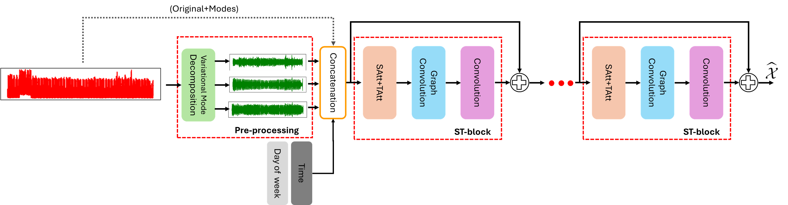
Figure 3: Block diagram of the variational mode graph convolutional network (VMGCN). The data is decomposed into components using VMD which are then concatenated as the features along the time of the day and day of the week. The original signal can also be concatenated in architecture variants and pass these modified features graph into a neural network. A spatio-temporal (ST) block applies SAtt: Spatial attention, TAtt: temporal attention, graph convolution, and time convolution. The prediction outcome $\hat{\mathcal{X}}\in\mathbb{R}^{N\times T_{w}}$ of VMGCN contains the future traffic flow from the timestamp of ($T_{w}+1$) to ($T_{w}+N_{H}$).

III-B Architecture Detail

The architecture of the framework, as illustrated in Fig. 3, consists primarily of two steps: pre-processing and learning. In the initial stage of this architecture, the time series signal of each node is decomposed into $K$ modes or components. The number of modes $K$ is a hyper-parameter that must be adjusted based on the nature of the dataset. After recursively decomposing the signal, the decomposed components are concatenated along with additional features $d^{{}^{\prime}}$ such as time of the day and day of the week. The new features of the graph is formed into $\tilde{\mathcal{X}}\in\mathbb{R}^{N\times(K+d^{{}^{\prime}})\times T}$.

The spatio-temporal (ST) block comprises spatial and temporal attention, graph convolution, and time convolution. Spatial and temporal attention mechanisms are applied to capture spatio-temporal correlations. Graph neural networks (GNNs) analyze the topological attributes of the graph and Chebyshev graph convolution (ChebNet) captures the properties of the graph for the Laplacian matrix in the spectral domain. Time convolution is employed to capture the temporal relationships within the graph structure. A residual connection combines the original feature with the output of the ST block, and 2D convolution is applied to its outcome. Multiple ST blocks are stacked together to obtain the final predicted outcome from the model.

IV Experiments

We perform our analysis for the following three case scenarios

• VMGCN-v1: Features include original signal, modes, and time information.

• VMGCN-v2: Features include modes and time information.

• VMGCN-v3: Features include redemption function $\phi(t)$, modes, and time information.

We compute the mean absolute percentage error (MAPE), mean absolute error (MAE), and root mean square error (RMSE) metrics to evaluate the performance of the proposed network. Before analyzing the performance of our proposed model, we will first provide a brief description of the dataset and the baseline models.

IV-A Datasets and Implementation Details

LargeST Dataset

In this work, for evaluation purposes, LargeST [36] dataset is used. It consists of a total of $8600$ nodes that are divided into four categories based on location: Greater Los Angeles (GLA), Greater Bay Areas (GBA), San Diego (SD), and others. It contains the traffic counts with a time interval of 5 minutes from 2017-2021. It also comprises meta-features such as longitude, latitude, and number of lanes.

Implementation Details

The experiments are performed on a Linux system equipped with an Intel(R) i9 24 GB RAM and NVIDIA 3080Ti GPU. The model is trained for a one-year duration of $2019$ where the samples are aggregated with a sample size of 15 minutes. The distribution of train, validation, and test is 60$\%$, $20\%$, $20\%$, respectively. The input horizon is $12$ and the horizon for prediction is also $12$. In this work, we are predicting the long-term traffic for the next $3$ hours. The proposed methods are implemented using PyTorch and used vmdpy tool for decomposition [39]. The batch size for the SD region is 64, GLA region is 8, and GBA region is 4. Each model is trained using the Adam optimizer for 100 epochs with early stopping criteria.

TABLE I: Distribution of nodes in LargeST where B (billion): $10^{9}$. Edges: Total number of edges between the nodes in the region, Degree: the average degree in each node.

Source	Dataset	Nodes	Edges	Degree	Data Points
LargeST	CA	$\mathbf{8,600}$	$\mathbf{201,363}$	$\mathbf{23.4}$	$\mathbf{4.52B}$
	GLA	$\mathbf{3,834}$	$\mathbf{98,703}$	$\mathbf{25.7}$	$\mathbf{2.02B}$
	GBA	$\mathbf{2,352}$	$\mathbf{61,246}$	$\mathbf{26.0}$	$\mathbf{1.24B}$
	SD	$\mathbf{716}$	$\mathbf{17,319}$	$\mathbf{24.2}$	$\mathbf{0.38B}$

IV-B Baseline Models

• Historical last (HL) [40] is a naive method that makes predictions based on the last observation.

• Long short-term memory (LSTM) [41], is a variant of RNN to capture large temporal dependencies.

• Diffusion convolutional recurrent neural networks (DCRNN) [12] captures the spatial and temporal pattern using diffusion convolution and encoding-decoding architecture respectively.

• Adaptive graph convolutional recurrent networks (AGCRN) [7] determines the node-specific spatial and temporal correlation in traffic series.

• Graph WaveNet (GWNET) [6] is a GNN architecture for spatial-temporal modeling.

• Spatial-temporal graph ode networks (STGODE) [10] extracts the dynamical pattern from traffic data using ordinary differential equation (ODE).

• Dynamic spatial-temporal aware graph neural networks (DSTAGNN) [19] constructs the data-driven graph and represents the spatial relevance using multi-head attention mechanism and temporal via gated convolution.

• Dynamic graph convolutional recurrent networks (DGCRN) [9] employs a mechanism to generate the dynamical topology of a graph for traffic prediction.

• Decoupled dynamic spatial-temporal graph neural networks (D²STGNN) [8] incorporates the decoupling of the traffic data in the learning mechanism.

• Attention-based spatial-temporal graph convolutional networks (ASTGCN) [11] introduces the attention mechanism and applies the graph convolution and temporal convolution in the modeling of ST data.

IV-C Analysis

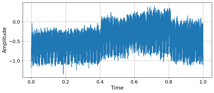
(a) $f(t)$

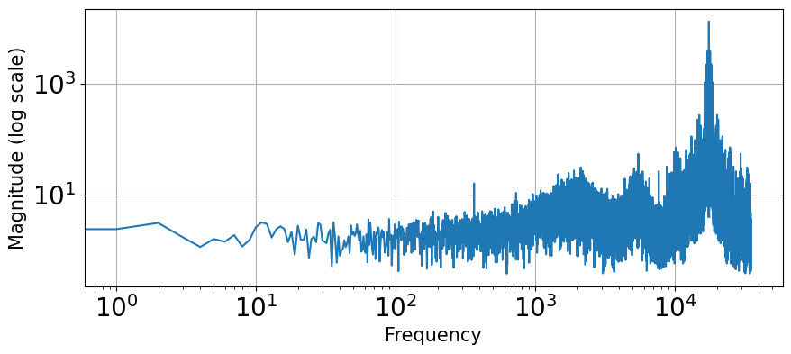
(b) $\sum\limits_{i=0}^{8}\lvert\hat{u_{i}}(\omega)\rvert$

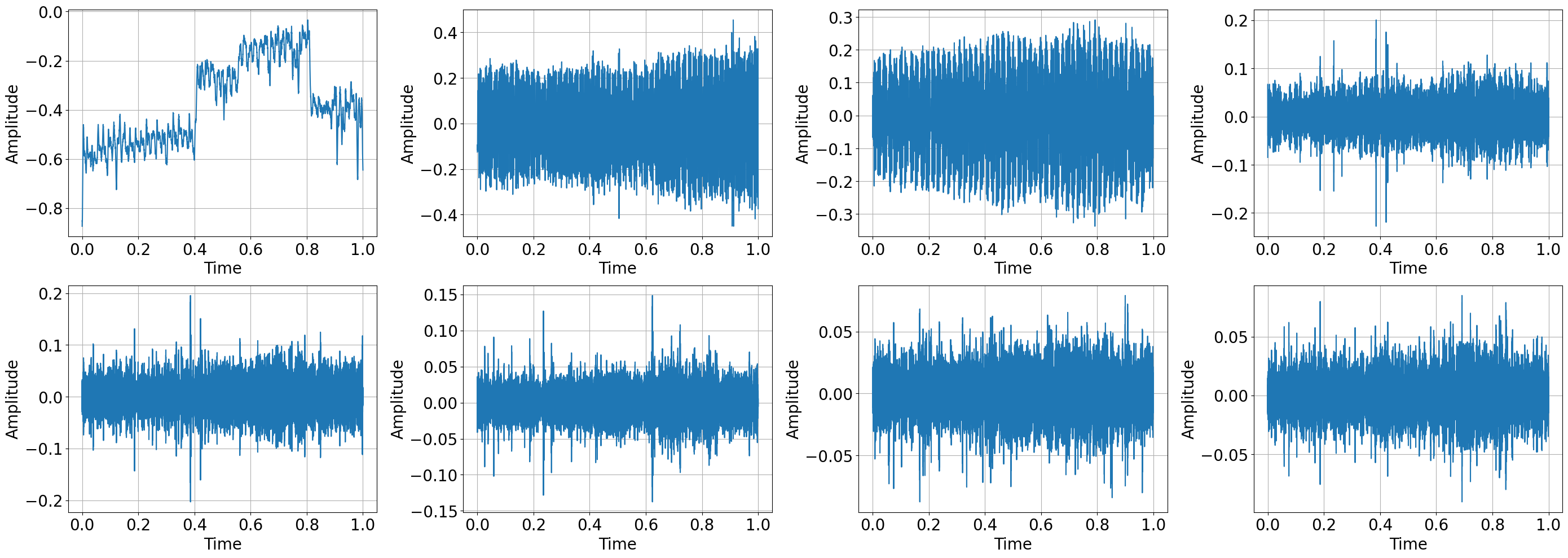
(c) VMD $u_{k}(t)$

Figure 4: Traffic signal decomposition. a) The normalized traffic signal of a sensor b) the spectrum of the magnitude of the reconstructed signal from modes. c) IMF1 - IMF8 plotted from lowest to highest-frequency components from top to bottom, left to right order.

VMD recursively decomposes traffic data into modes that can be categorized into high-frequency, intermediate, and low-frequency components. These modes represent the real-time non-stationary and complex nature of the signals, which consist of numerous modes, as depicted in Fig. 4. Fig. 4(a) displays the counts from a 1-year traffic sensor in the SD region. The pattern of periodic, quasi-periodic, and noise components in the signal spectrum is illustrated in Fig. 4(b). The signal is segregated into 8 modes, shown in Fig. 4(c) ordered from low to high frequencies (IMF1 - IMF8). These modes can have physical interpretation in real-time traffic analysis. The lowest-frequency mode (IMF1) mimics the overall trend of the original signal at low frequency, while the highest-frequency mode (IMF8) describes the noise in the signal. The number of intermediate-frequency modes may vary depending on the total number of modes and the complexity of the signal. The noise-free signal can be reconstructed by summing the components, excluding the lowest-frequency and highest-frequency modes, as referenced in [31].

The tuning of hyper-parameters remains a crucial step in the training process of a deep learning model. In the decomposition of data, it is essential to select the appropriate values for the number of modes ($K$), bandwidth constraint ($\alpha$), tolerance for convergence ($\epsilon$), and total iteration ($N_{H}$) for VMD. The performance of our proposed method has been evaluated under different values of $K$ modes. Fig. 5 shows the MAE training loss evaluated on the SD region of the LargeST dataset, while keeping the other hyper-parameters constant. It shows that the loss gradually decreases as the number of modes increases. However, finding the suitable value of $K$ that yields the best prediction results is computationally expensive. Consequently, we have formulated a method that utilizes reconstruction loss based on the threshold ($\zeta$) criteria.

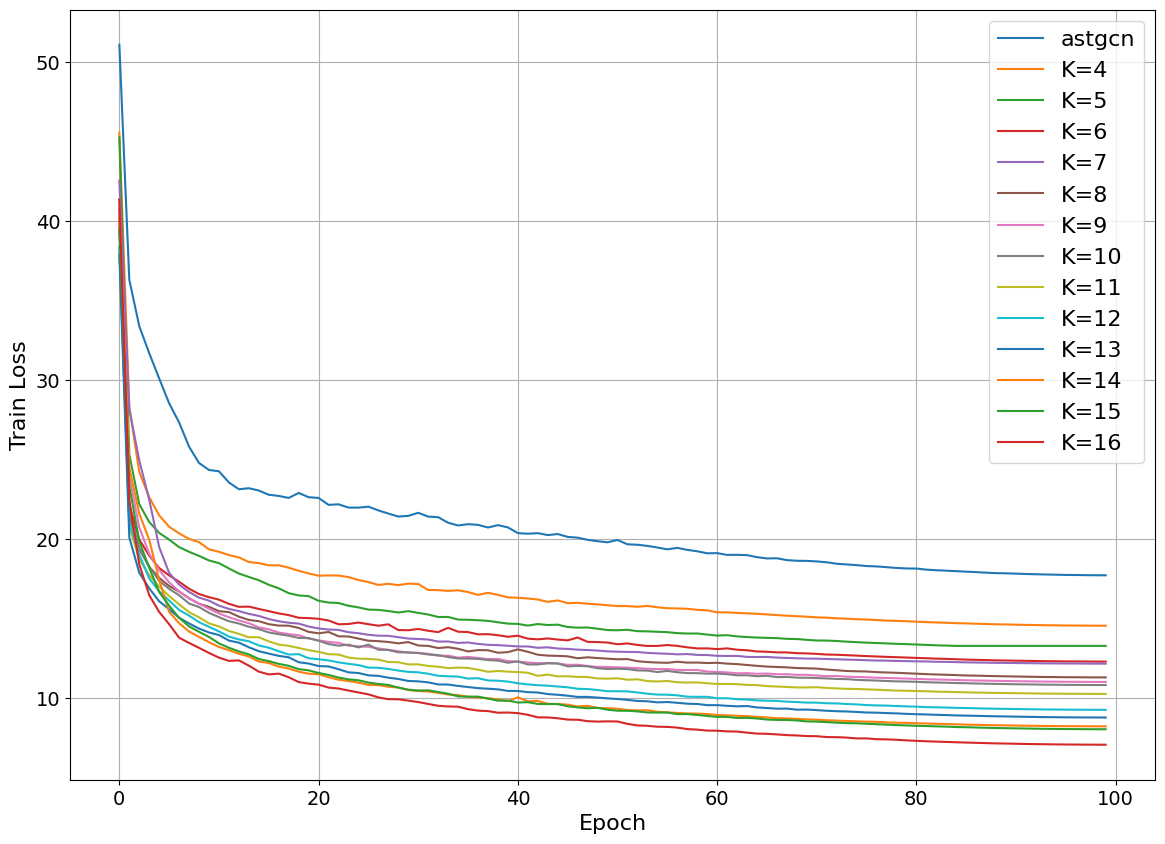
Figure 5: Training loss with different modes on SD dataset for VMGCN-v1. It shows that the training loss decreases with the increase in the number of modes.

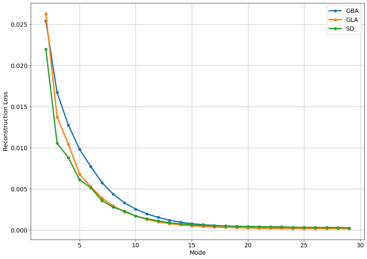
Figure 6: The sub-optimal number of modes is determined by randomly selecting signal and performing decomposition for mode range $[2,29]$. If the mean reconstruction loss of the signals is less than a threshold value on a specific mode, consider that mode as a sub-optimal value.

To determine the best-fit number of mode, we randomly select the nodes and compute the modes and for each, subsequently calculating the average reconstruction loss of the sample data for every $K$ value. If the reconstruction loss is less than the threshold value ($\zeta$), we can consider this $K$ value as a near-best term. In our experimentation, we selected $2\%$ of the nodes from each region and applied this method for $K$ values ranging from $2$ to $29$, as shown in Fig. 6. The best value of $K$ is identified for each region: SD $K=13$, GBA $K=14$, GLA $K=13$ when the reconstruction loss is less than the $\zeta=1\times 10^{-3}$. After identifying the $K$ value for each region, it is observed that any further decrease in loss beyond these values is negligible.

TABLE II: Comparison of performance evaluation metrics MAE, MAPE, and RMSE between different advanced methods and our models. The number of parameters (param) is described in K (kilo), $10^{3}$ and M (million), $10^{6}$, and the best performance metrics are highlighted in red bold numbers. For VMGCN-vx-$K$, x describes the variant of the network and $K$ corresponds to the best value chosen for each region.

Dataset	Method	Param	Horizon 3			Horizon 6			Horizon 12			Average
			MAE	RMSE	MAPE	MAE	RMSE	MAPE	MAE	RMSE	MAPE	MAE	RMSE	MAPE
SD	HL’	-	33.61	50.97	20.77%	57.80	84.92	37.73%	101.74	140.14	76.84%	60.79	87.40	41.88%
	LSTM’	98K	19.17	30.75	11.85%	26.11	41.28	16.53%	38.06	59.63	25.07%	26.73	42.14	17.17%
	DCRNN’	373K	17.01	27.33	10.96%	20.80	33.03	13.72%	26.77	42.49	18.57%	20.86	33.13	13.94%
	AGCRN’	761K	16.05	28.78	11.74%	18.37	32.44	13.37%	22.12	40.37	16.63%	18.43	32.97	13.51%
	STGCN’	508K	18.23	30.60	13.75%	20.34	34.42	15.10%	23.56	41.70	17.08%	20.35	34.70	15.13%
	GWNET’	311K	15.49	25.45	9.90%	18.17	30.16	11.98%	22.18	37.82	15.41%	18.12	30.21	12.08%
	STGODE’	729K	16.76	27.26	10.95%	19.79	32.91	13.18%	23.60	41.32	16.60%	19.52	32.76	13.22%
	DSTAGNN’	3.9M	17.83	28.60	11.08%	21.95	35.37	14.55%	26.83	46.39	19.62%	21.52	35.67	14.52%
	DGCRN’	243K	15.24	25.46	10.09%	17.66	29.65	11.77%	21.59	35.55	16.88%	17.38	28.92	12.43%
	D2STGNN”	406K	15.76	25.71	11.84%	18.81	30.68	14.39%	23.17	38.76	18.13%	18.71	30.77	13.99%
	ASTGCN”	2.15M	19.68	31.53	12.20%	24.45	38.89	15.36%	31.52	49.77	22.15%	26.07	38.42	15.63%
	VMGCN-v1-13”	2.17M	5.09	13.08	4.71%	8.93	36.31	9.13%	20.10	100.37	19.23%	11.28	47.61	10.21%
	VMGCN-v2-13”	2.17M	5.62	9.21	5.19%	10.27	17.00	9.04%	18.59	31.73	18.15%	10.84	18.26	10.10%
	VMGCN-v3-13”	2.17M	6.20	9.80	5.51%	11.22	17.66	9.08%	18.33	28.12	15.46%	11.29	17.65	9.39%
GBA	HL’	-	32.57	48.42	22.78%	53.79	77.08	43.01%	92.64	126.22	92.85%	56.44	79.82	48.87%
	LSTM’	98K	20.41	33.47	15.60%	27.50	43.64	23.25%	38.85	60.46	37.47%	27.88	44.23	24.31%
	DCRNN’	373K	18.25	29.73	14.37%	22.25	35.04	19.82%	28.68	44.39	28.69%	22.35	35.26	20.15%
	AGCRN’	777K	18.11	30.19	13.64%	20.86	34.42	16.24%	24.06	39.47	19.29%	20.55	33.91	16.06%
	STGCN’	1.3M	20.62	33.81	15.84%	23.19	37.96	18.09%	26.53	43.88	21.77%	23.03	37.82	18.20%
	GWNET’	344K	17.74	28.92	14.37%	20.98	33.50	17.77%	25.39	40.30	22.99%	20.78	33.32	17.76%
	STGODE’	788K	18.80	30.53	15.67%	22.19	35.91	18.54%	26.27	43.07	22.71%	21.86	35.57	17.76%
	DSTAGNN’	26.9M	19.87	31.54	16.85%	23.89	38.11	19.53%	28.48	44.65	24.65%	23.39	37.07	19.58%
	DGCRN’	374K	18.09	29.27	15.32%	21.18	33.78	18.59%	25.73	40.88	23.67%	21.10	33.76	18.58%
	D2STGNN’	446K	17.20	28.50	12.22%	20.80	33.53	15.32%	25.72	40.90	19.90%	20.71	33.44	15.23%
	ASTGCN’	22.30M	21.40	33.61	17.65%	26.70	40.75	24.02%	33.64	51.21	31.15%	26.15	40.25	23.29%
	VMGCN-v1-14”	22.38M	2.90	5.32	3.27%	6.47	11.62	6.86%	16.42	26.45	17.55%	8.04	13.55	8.57%
	VMGCN-v2-14”	22.38M	3.67	6.34	4.16%	7.05	12.25	7.57%	17.24	27.22	18.58%	8.75	14.37	9.41%
	VMGCN-v3-14”	22.38M	3.58	6.24	4.06%	7.06	12.31	7.66%	17.47	27.66	18.54%	8.77	14.45	9.42%
GLA	HL’	-	33.66	50.91	19.16%	56.88	83.54	34.85%	98.45	137.52	71.14%	56.58	86.19	38.76%
	LSTM’	98K	20.09	32.41	11.82%	27.80	44.10	16.52%	39.61	61.57	25.63%	28.12	44.40	17.31%
	DCRNN’	373K	18.33	29.13	10.78%	22.70	35.55	13.74%	29.45	45.88	18.87%	22.73	35.65	13.97%
	AGCRN’	792K	17.57	30.83	10.86%	20.79	36.09	13.11%	25.01	44.82	16.11%	20.61	36.23	12.99%
	STGCN’	2.1M	19.87	34.01	12.58%	22.54	38.57	13.94%	26.48	45.61	16.92%	22.48	38.55	14.15%
	GWNET’	374K	17.30	27.72	10.69%	21.22	33.64	13.48%	27.25	43.03	18.49%	21.23	33.68	13.72%
	STGODE’	841K	18.46	30.05	11.94%	22.24	36.68	14.67%	27.14	45.38	19.12%	22.02	36.34	14.93%
	DSTAGNN’	66.3M	19.35	30.55	11.33%	24.22	38.19	15.90%	230.32	48.37	23.51%	23.87	37.88	15.36%
	DGCRN’	432K	17.63	8.12	10.50%	21.15	33.70	13.06%	26.18	42.16	17.40%	21.02	33.66	13.23%
	D2STGNN’	284K	19.31	30.07	11.82%	22.52	35.22	14.16%	27.46	43.37	18.54%	22.35	35.11	14.37%
	ASTGCN’	59.1M	21.11	32.41	11.82%	27.80	44.67	17.79%	39.39	59.31	28.03%	28.12	44.40	18.62%
	VMGCN-v1-13”	59.2M	3.88	10.78	3.99%	8.27	22.34	7.85%	16.78	31.46	14.28%	9.22	20.69	8.23%
	VMGCN-v2-13”	59.2M	4.54	11.47	4.58%	8.75	21.60	8.54%	18.21	32.56	16.39%	9.99	21.10	9.17%
	VMGCN-v3-13”	59.2M	4.62	11.54	4.65%	8.84	21.51	8.65%	17.98	31.53	15.57%	9.98	20.78	9.09%

• results executed by [36].

• results executed by us.

The comparison of our experimentation with baseline models is presented in TABLE II. We evaluated our case scenarios using $\alpha=2000$, $\epsilon=1\times 10^{-7}$, and $N_{H}=500$. For VMGCN-v1, incorporating the original feature with the modes generally leads to better predictions. In long-horizon prediction, VMGCN-v3 exhibits relatively lower error values compared to VMGCN-v2. The decomposition by VMD is sensitive to the length of the signal. Currently, utilizing the 1-year data makes the computed modes more effective. Typical traffic trends such as jams, congestion, and daily, or weekly patterns are well-defined in terms of frequencies. Due to the accurate representation of features, the neural networks predict future states. Increasing the number of modes enhances the performance of the model in short-term prediction, but it tends to overfit in long-term predictions. It appears that VMD effectively decomposes the signal at higher modes and removes noise, leading to more precise immediate prediction.

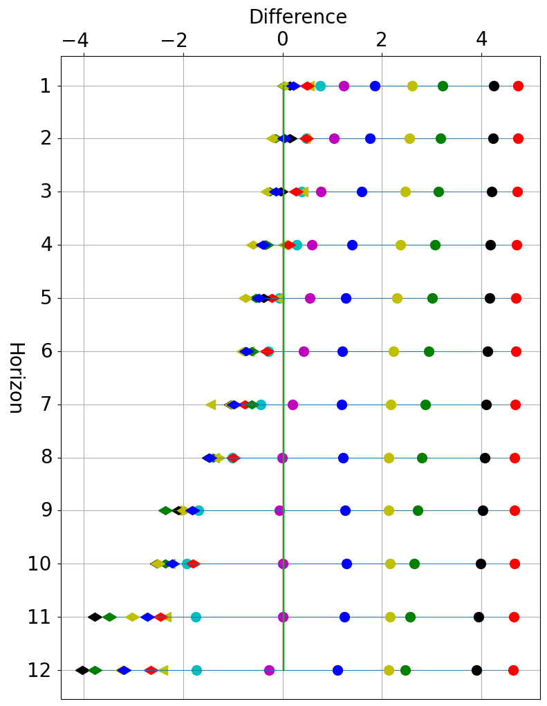
(a) MAE

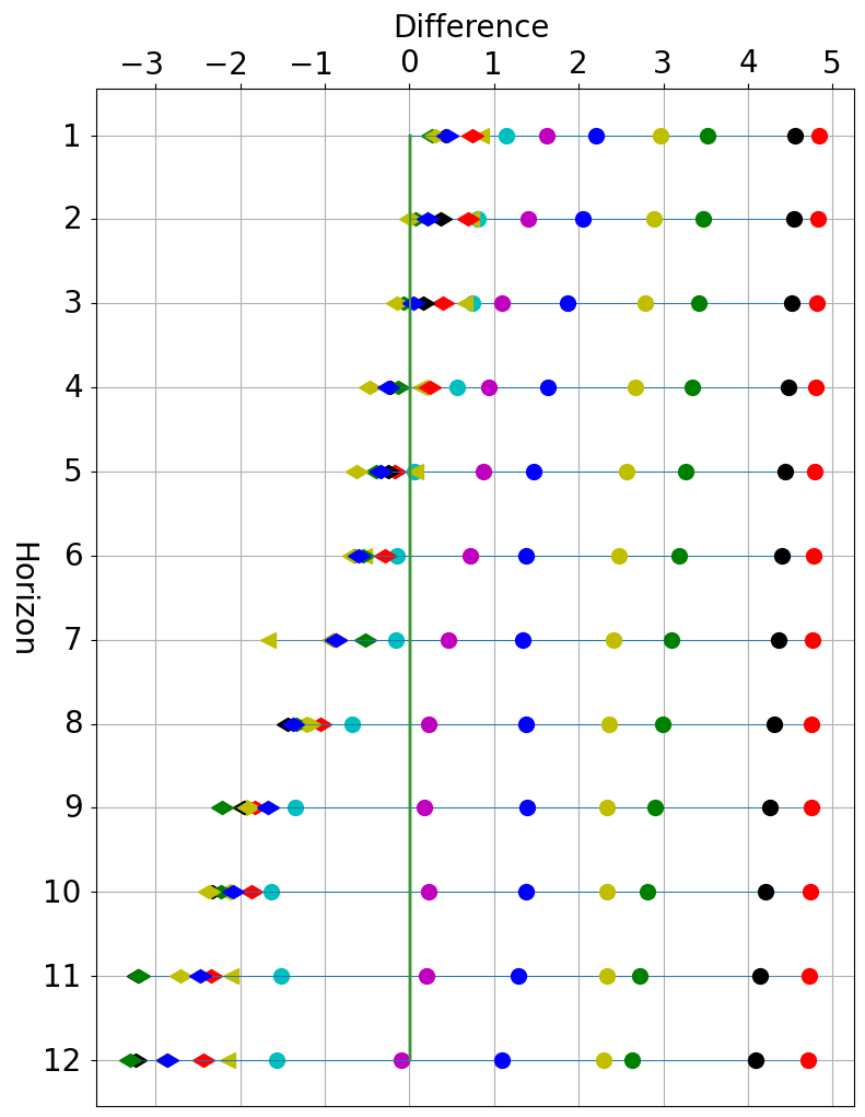
(b) RMSE

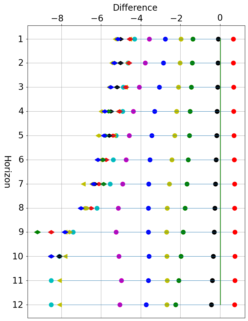
(c) MAPE

Figure 7: The importance of each mode in horizon prediction is studied by replacing the respective mode with zero value and performing inference to observe the change in the performance metrics. The plot shows the differences in metrics between the original and distorted modes on the logarithmic scale. The greater the difference, the more significant the mode for that horizon. This analysis has been performed on the SD region for VMGCN-v2.

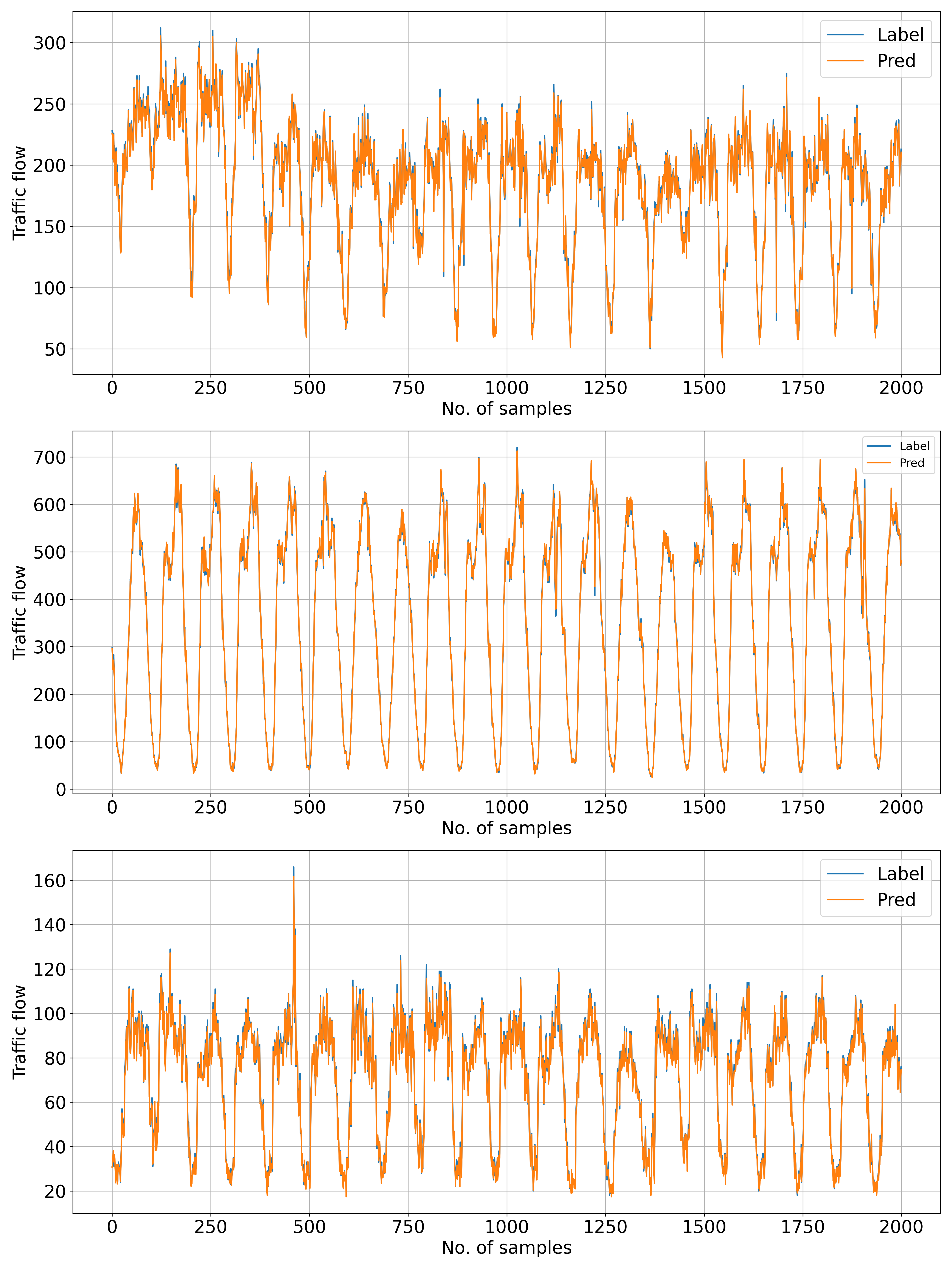
Figure 8: This plot shows the comparison of ground truth with the predicted traffic flow for horizon 1 on three distinct locations in the SD region.

To evaluate the effectiveness of each mode on horizon prediction, the modes are analyzed in terms of central frequencies and energy. This relationship between prediction accuracy and the modes, separated based on frequencies, is investigated in Fig. 7. In VMGCN-v2 for the SD region, inference is performed by setting each mode to zero in the test set. The Fig. 7(a), 7(b), and 7(c) show the logarithm of non-zero $\Delta$ MAE, $\Delta$ RMSE, and $\Delta$ MAPE repeativety for all horizons, respectively. Here, $\Delta$ represents the difference between the metric with all features and the metric with zero value in $k^{\rm{th}}$ mode for a horizon. The modes from $1$ to $13$ are arranged in terms of increasing frequency components. A higher metric value signifies the importance of that mode in horizon prediction. It has been observed that lower-frequency components contribute more to prediction accuracy relative to high-frequency components. As frequency increases, the noise in the mode also increases, and the pattern useful for prediction decreases. Removing the high-frequency components during the training of the neural network could potentially enhance the capabilities of the model performance.

We also compare the predicted traffic flow and the actual flow for Horizon $1$ plotted in Fig. 8 for three sensors at different locations. The model under-predicts some values at the peak times, which correspond to rush hours. Sensors 2 and 3 exhibit some periodic trends with harmonic noise.

TABLE III: Performance evaluation of metrics MAE, MAPE, and RMSE

Description	Hyper-Parameters	Reconstruction Loss	Horizon 3			Horizon 6			Horizon 12			Average
			MAE	RMSE	MAPE	MAE	RMSE	MAPE	MAE	RMSE	MAPE	MAE	RMSE	MAPE
VMGCN-v2	$\alpha=2000,\epsilon=10^{-7}$	$9.53\times 10^{-4}$	5.62	9.21	5.19%	10.27	17.00	9.04%	18.59	31.73	18.15%	10.84	18.26	10.10%
VMGCN-v2	$\alpha=2000,\epsilon=10^{-6}$	$9.53\times 10^{-4}$	5.48	8.91	5.13%	10.07	16.00	8.47%	17.46	26.89	14.99%	10.42	16.34	8.92%
VMGCN-v2	$\alpha=1000,\epsilon=10^{-7}$	$3.22\times 10^{-4}$	4.25	7.76	4.06%	8.65	14.40	7.79%	17.56	26.57	15.55%	9.43	15.10	8.46%
VMGCN-v2	$\alpha=1000,\epsilon=10^{-6}$	$3.22\times 10^{-4}$	4.17	7.74	3.96%	8.45	14.30	7.59%	16.77	25.86	14.83%	9.41	14.90	8.16%
VMGCN-v1(without IMF13)	$\alpha=2000,\epsilon=10^{-7}$	$1.51\times 10^{-3}$	4.83	8.19	4.33%	9.41	15.11	7.40%	15.15	23.56	12.33%	9.34	14.92	7.49%

IV-D Ablative Study

The performance of the framework has been evaluated on various combinations of decomposition hyper-parameters such as $\alpha$, and $\epsilon$, for the SD region. TABLE III details different performance metrics for horizons $3$, $6$, and $12$, and the average. It has been observed that for $\alpha=1000$, the reconstruction loss is relatively lower compared to $\alpha=2000$. Changing the $\epsilon$ value does not significantly affect the reconstruction loss, indicating that the convergence is sensitive to initial conditions, which may lead to local minima instead of global minimum. For VMGCN-v2, it is noticed that decreasing the bandwidth constraint and increasing the tolerance value improves the performance metrics. The overall cumulative effect on the reconstruction loss term in the region remains unaffected by changes in the $\epsilon$ term. However, the difference in the reconstructed loss term of modes defined as

$$\frac{1}{L}\lvert\sum_{i}u(t)_{i,\epsilon 1}-\sum_{i}u(t)_{i,\epsilon 2}\rvert,$$ (14)

where $L$ is the total length of the signal. For this comparison, we used $\epsilon_{1}=1\times 10^{-7}$ and $\epsilon_{2}=1\times 10^{-6}$. With a bandwidth constraint of $\alpha=1000$, the loss term is measured as $1.134\times 10^{-5}$, indicating a convergence difference between these sets of decomposition parameters, with different local minima being reached. The framework performs better with $\epsilon_{2}$ compared to $\epsilon_{1}$. If the bandwidth constraint is set at $\alpha=2000$, the $L_{1}$ loss term of the mode approaches zero, indicating that at a larger bandwidth value, the role of tolerance in convergence is less significant. From the table, we may also infer that changing the bandwidth constraint has a dominant impact on the performance of the network. By eliminating the high-frequency (IMF13) in VMGCN-v1, the DNN is trained and evaluates the performance of the model. It appears that the overall performance of the network is enhanced, specifically the long-term predictions. The high-frequency component adversely affects the long-term prediction capabilities of the network.

IV-E Computational Complexity

In TABLE II, we compare the number of parameters of our framework, which includes $K$ modes and additional features, with the state-of-the-art ASTGCN method. It shows that the increase in parameters by adding features to the traffic flow is negligible. However, the time complexity in decoupling the traffic counts takes a significant amount of time relative to training the model. The complexity $\mathcal{O}$ in terms of time for each element of an ST block in ASTGCN is formulated in this section. Typically, $N\gg d$ and $N\gg T_{w}$ for targeted traffic prediction applications. The time complexity for normalized spatial attention $\mathbf{S}^{{}^{\prime}}$ is $\mathcal{O}(N^{3})$. The complexity for normalized temporal attention is $\mathcal{O}(NdT_{w})$, for Chebyshev convolution is $\mathcal{O}(T_{w}MN^{2}C)$, and for time convolution is $\mathcal{O}(FO_{h}O_{w}K_{h}K_{w}C)$, where

$$O_{h}=\bigg{\lfloor}\frac{N-K_{h}}{S_{h}}\bigg{\rfloor}+1,$$

$$O_{w}=\bigg{\lfloor}\frac{T-K_{w}}{S_{w}}\bigg{\rfloor}+1,$$

are the height and width of the output tensors of the 2D convolution, respectively. The width and height of the kernel are described by $K_{w}$ and $K_{h}$, and the strides of the convolution are described by $S_{w}$ and $S_{h}$. The number of the output filter $F$ of CNN and $C$ is the number of the Chebyshev channel. If we have the $B$ number of ST blocks in ASTGCN, the complexity will be $\mathcal{O}(B(N^{3}+NdT_{w}+T_{w}MN^{2}C+FO_{h}O_{w}K_{h}K_{w}C))$.

The computational complexity for the VMD includes: mirroring of the signal is $\mathcal{O}(L)$, the FFT $\mathcal{O}(L\log L)$, the update of the modes $\mathcal{O}(N_{\rm{iter}}KL)$, and the reconstruction of the signal is $\mathcal{O}(KL\log(L))$. Considering the number of iterations $N_{\rm{iter}}=500$, the overall complexity of VMD for all nodes is $\mathcal{O}(NN_{\rm{iter}}KL)$. It shows that the update of modes $u_{k}(\omega)$ and central frequencies $\omega_{k}$ quantify the computation cost of the decomposition of the signal.

Due to this limitation, our framework is well-suited for offline prediction of the ST data because we are decomposing the 1-year data rather than input samples. The computation of the decomposition of the signal can be optimized and made learnable by using deep unrolling of the VMD algorithm. This proposed approach can be implemented for future modifications of the framework.

V Conclusion

In this work, we successfully implemented a hybrid method for both short-term and long-term spatio-temporal (ST) forecasting. The ST data is decomposed into modes, which are then used as features for the deep-learning model to predict future states. The number of modes for real-time applications is determined using the reconstruction loss. The low-frequency modes significantly contribute to horizon prediction while high-frequency modes contain the noise from the signal. By discarding the highest frequency mode from the features, we can enhance the prediction accuracy. However, the bandwidth and tolerance values significantly influence the convergence and performance of our proposed framework. We evaluated the performance of our architecture on the traffic flow dataset, it outperforms in both short and long-term prediction compared to state-of-the-art methods.

References

- [1] Ammar Haydari and Yasin Yılmaz, “Deep reinforcement learning for intelligent transportation systems: A survey,” IEEE Transactions on Intelligent Transportation Systems, vol. 23, no. 1, pp. 11–32, 2020.
- [2] Mohammad M Hamed, Hashem R Al-Masaeid, and Zahi M Bani Said, “Short-term prediction of traffic volume in urban arterials,” Journal of Transportation Engineering, vol. 121, no. 3, pp. 249–254, 1995.
- [3] Iwao Okutani and Yorgos J Stephanedes, “Dynamic prediction of traffic volume through kalman filtering theory,” Transportation Research Part B: Methodological, vol. 18, no. 1, pp. 1–11, 1984.
- [4] Brian L Smith, Billy M Williams, and R Keith Oswald, “Comparison of parametric and nonparametric models for traffic flow forecasting,” Transportation Research Part C: Emerging Technologies, vol. 10, no. 4, pp. 303–321, 2002.
- [5] Hinsbergen et al., Artificial Intelligence Applications to Critical Transportation Issues, Transportation Research Board, 2012.
- [6] Zonghan Wu, Shirui Pan, Guodong Long, Jing Jiang, and Chengqi Zhang, “Graph wavenet for deep spatial-temporal graph modeling,” arXiv preprint arXiv:1906.00121, 2019.
- [7] Lei Bai, Lina Yao, Can Li, Xianzhi Wang, and Can Wang, “Adaptive graph convolutional recurrent network for traffic forecasting,” Advances in neural information processing systems, vol. 33, pp. 17804–17815, 2020.
- [8] Zezhi Shao, Zhao Zhang, Wei Wei, Fei Wang, Yongjun Xu, Xin Cao, and Christian S Jensen, “Decoupled dynamic spatial-temporal graph neural network for traffic forecasting,” arXiv preprint arXiv:2206.09112, 2022.
- [9] Fuxian Li, Jie Feng, Huan Yan, Guangyin Jin, Fan Yang, Funing Sun, Depeng Jin, and Yong Li, “Dynamic graph convolutional recurrent network for traffic prediction: Benchmark and solution,” ACM Transactions on Knowledge Discovery from Data, vol. 17, no. 1, pp. 1–21, 2023.
- [10] Zheng Fang, Qingqing Long, Guojie Song, and Kunqing Xie, “Spatial-temporal graph ode networks for traffic flow forecasting,” in Proceedings of the 27th ACM SIGKDD conference on knowledge discovery & data mining, 2021, pp. 364–373.
- [11] Shengnan Guo, Youfang Lin, Ning Feng, Chao Song, and Huaiyu Wan, “Attention based spatial-temporal graph convolutional networks for traffic flow forecasting,” in Proceedings of the AAAI conference on artificial intelligence, 2019, vol. 33, pp. 922–929.
- [12] Yaguang Li, Rose Yu, Cyrus Shahabi, and Yan Liu, “Diffusion convolutional recurrent neural network: Data-driven traffic forecasting,” arXiv preprint arXiv:1707.01926, 2017.
- [13] Yuxuan Zhang, Senzhang Wang, Bing Chen, Jiannong Cao, and Zhiqiu Huang, “Trafficgan: Network-scale deep traffic prediction with generative adversarial nets,” IEEE Transactions on Intelligent Transportation Systems, vol. 22, no. 1, pp. 219–230, 2019.
- [14] Jifeng Dai, Haozhi Qi, Yuwen Xiong, Yi Li, Guodong Zhang, Han Hu, and Yichen Wei, “Deformable convolutional networks,” in Proceedings of the IEEE international conference on computer vision, 2017, pp. 764–773.
- [15] Yingxue Zhang, Yanhua Li, Xun Zhou, Xiangnan Kong, and Jun Luo, “Curb-gan: Conditional urban traffic estimation through spatio-temporal generative adversarial networks,” in Proceedings of the 26th ACM SIGKDD International Conference on Knowledge Discovery & Data Mining, 2020, pp. 842–852.
- [16] Ziqian Lin, Jie Feng, Ziyang Lu, Yong Li, and Depeng Jin, “Deepstn+: Context-aware spatial-temporal neural network for crowd flow prediction in metropolis,” in Proceedings of the AAAI conference on artificial intelligence, 2019, vol. 33, pp. 1020–1027.
- [17] Ling Cai, Krzysztof Janowicz, Gengchen Mai, Bo Yan, and Rui Zhu, “Traffic transformer: Capturing the continuity and periodicity of time series for traffic forecasting,” Transactions in GIS, vol. 24, no. 3, pp. 736–755, 2020.
- [18] Xuesong Nie, Xi Chen, Haoyuan Jin, Zhihang Zhu, Yunfeng Yan, and Donglian Qi, “Triplet attention transformer for spatiotemporal predictive learning,” in Proceedings of the IEEE/CVF Winter Conference on Applications of Computer Vision, 2024, pp. 7036–7045.
- [19] Shiyong Lan, Yitong Ma, Weikang Huang, Wenwu Wang, Hongyu Yang, and Pyang Li, “Dstagnn: Dynamic spatial-temporal aware graph neural network for traffic flow forecasting,” in International conference on machine learning. PMLR, 2022, pp. 11906–11917.
- [20] Zheyi Pan, Yuxuan Liang, Weifeng Wang, Yong Yu, Yu Zheng, and Junbo Zhang, “Urban traffic prediction from spatio-temporal data using deep meta learning,” in Proceedings of the 25th ACM SIGKDD international conference on knowledge discovery & data mining, 2019, pp. 1720–1730.
- [21] Bing Yu, Haoteng Yin, and Zhanxing Zhu, “Spatio-temporal graph convolutional networks: A deep learning framework for traffic forecasting,” arXiv preprint arXiv:1709.04875, 2017.
- [22] Ashish Vaswani, Noam Shazeer, Niki Parmar, Jakob Uszkoreit, Llion Jones, Aidan N Gomez, Łukasz Kaiser, and Illia Polosukhin, “Attention is all you need,” Advances in neural information processing systems, vol. 30, 2017.
- [23] Kuo Wang, LingBo Liu, Yang Liu, GuanBin Li, Fan Zhou, and Liang Lin, “Urban regional function guided traffic flow prediction,” Information Sciences, vol. 634, pp. 308–320, 2023.
- [24] Yue Hou, Zhiyuan Deng, and Hanke Cui, “Short-term traffic flow prediction with weather conditions: Based on deep learning algorithms and data fusion,” Complexity, vol. 2021, no. 1, pp. 6662959, 2021.
- [25] Yuhan Jia, Jianping Wu, Moshe Ben-Akiva, Ravi Seshadri, and Yiman Du, “Rainfall-integrated traffic speed prediction using deep learning method,” IET Intelligent Transport Systems, vol. 11, no. 9, pp. 531–536, 2017.
- [26] Xusen Guo, Qiming Zhang, Junyue Jiang, Mingxing Peng, Hao Frank Yang, and Meixin Zhu, “Towards responsible and reliable traffic flow prediction with large language models,” Available at SSRN 4805901, 2024.
- [27] Norden E Huang, Zheng Shen, Steven R Long, Manli C Wu, Hsing H Shih, Quanan Zheng, Nai-Chyuan Yen, Chi Chao Tung, and Henry H Liu, “The empirical mode decomposition and the hilbert spectrum for nonlinear and non-stationary time series analysis,” Proceedings of the Royal Society of London. Series A: mathematical, physical and engineering sciences, vol. 454, no. 1971, pp. 903–995, 1998.
- [28] Zhaohua Wu and Norden E Huang, “Ensemble empirical mode decomposition: a noise-assisted data analysis method,” Advances in adaptive data analysis, vol. 1, no. 01, pp. 1–41, 2009.
- [29] María E Torres, Marcelo A Colominas, Gaston Schlotthauer, and Patrick Flandrin, “A complete ensemble empirical mode decomposition with adaptive noise,” in 2011 IEEE international conference on acoustics, speech and signal processing (ICASSP). IEEE, 2011, pp. 4144–4147.
- [30] Naveed Rehman and Danilo P Mandic, “Multivariate empirical mode decomposition,” Proceedings of the Royal Society A: Mathematical, Physical and Engineering Sciences, vol. 466, no. 2117, pp. 1291–1302, 2010.
- [31] Konstantin Dragomiretskiy and Dominique Zosso, “Variational mode decomposition,” IEEE transactions on signal processing, vol. 62, no. 3, pp. 531–544, 2013.
- [32] Haichao Huang, Jingya Chen, Rui Sun, and Shuang Wang, “Short-term traffic prediction based on time series decomposition,” Physica A: Statistical Mechanics and its Applications, vol. 585, pp. 126441, 2022.
- [33] Guangxin Li and Xiang Zhong, “Parking demand forecasting based on improved complete ensemble empirical mode decomposition and gru model,” Engineering Applications of Artificial Intelligence, vol. 119, pp. 105717, 2023.
- [34] Jingyi Lu, “An efficient and intelligent traffic flow prediction method based on lstm and variational modal decomposition,” Measurement: Sensors, vol. 28, pp. 100843, 2023.
- [35] Kaixin Guo, Xin Yu, Gaoxiang Liu, and Shaohu Tang, “A long-term traffic flow prediction model based on variational mode decomposition and auto-correlation mechanism,” Applied Sciences, vol. 13, no. 12, pp. 7139, 2023.
- [36] Xu Liu, Yutong Xia, Yuxuan Liang, Junfeng Hu, Yiwei Wang, Lei Bai, Chao Huang, Zhenguang Liu, Bryan Hooi, and Roger Zimmermann, “Largest: A benchmark dataset for large-scale traffic forecasting,” Advances in Neural Information Processing Systems, vol. 36, 2024.
- [37] M. Seyed Kazemi, “Dynamic graph neural networks,” in Graph Neural Networks: Foundations, Frontiers, and Applications, Lingfei Wu, Peng Cui, Jian Pei, and Liang Zhao, Eds., pp. 323–349. Springer Singapore, Singapore, 2022.
- [38] Michaël Defferrard, Xavier Bresson, and Pierre Vandergheynst, “Convolutional neural networks on graphs with fast localized spectral filtering,” Advances in neural information processing systems, vol. 29, 2016.
- [39] Vinícius R Carvalho, Márcio FD Moraes, Antônio P Braga, and Eduardo MAM Mendes, “Evaluating five different adaptive decomposition methods for eeg signal seizure detection and classification,” Biomedical Signal Processing and Control, vol. 62, pp. 102073, 2020.
- [40] Yuxuan Liang, Kun Ouyang, Yiwei Wang, Ye Liu, Junbo Zhang, Yu Zheng, and David S Rosenblum, “Revisiting convolutional neural networks for citywide crowd flow analytics,” in Machine Learning and Knowledge Discovery in Databases: European Conference, ECML PKDD 2020, Ghent, Belgium, September 14–18, 2020, Proceedings, Part I. Springer, 2021, pp. 578–594.
- [41] Sepp Hochreiter and Jürgen Schmidhuber, “Long short-term memory,” Neural computation, vol. 9, no. 8, pp. 1735–1780, 1997.