The Standard Model of Particle Physics as an effective theory from two non-universal $U(1)$’s

Abstract

We study the possibility of obtaining the Standard Model (SM) of particle physics as an effective theory of a more fundamental one, whose electroweak sector includes two non-universal local $U(1)$ gauge groups, with the chiral anomaly cancellation taking place through an interplay among families. As a result of the spontaneous symmetry breaking, a massive gauge boson $Z^{\prime}$ arises, which couples differently to the third family of fermions (by assumption, we restrict ourselves to the scenario in which the $Z^{\prime}$ couples in the same way to the first two families). Two Higgs doublets and one scalar singlet are necessary to generate the SM fermion masses and break the gauge symmetries. We show that in our model, the flavor-changing neutral currents (FCNC) of the Higgs sector are identically zero if each right-handed SM fermion is only coupled with a single Higgs doublet. This result represents a FCNC cancellation mechanism different from the usual procedure in Two-Higgs Doublet Models (2HDM). The non-universal nature of our solutions requires the presence of three right-handed neutrino fields, one for each family. Our model generates all elements of the Dirac mass matrix for quarks and leptons, which is quite non-trivial for non-universal models. Thus, we can fit all the masses and mixing angles with two scalar doublets. Finally, we show the distribution of solutions for the scalar boson masses in our model by scanning well-motivated intervals for the model parameters. We consider two possibilities for the scalar potential and compare these results with the Higgs-like resonant signals recently reported by the ATLAS and CMS experiments at the LHC. Finally, we also report collider, electroweak, and flavor constraints on the model parameters.

1 Introduction

The Standard Model of particle physics based on the local gauge group $SU(3)_{\text{C}}\otimes SU(2)_{L}\otimes U(1)_{Y}$ [1] has been very successful so far, in the sense that its predictions are in good agreement with the present experimental results, including the latest discovery of the Higgs boson [2, 3, 4], a fundamental ingredient of the model that contributes to our understanding of the origin of mass for the subatomic particles. However, the SM fails short in explaining things as: hierarchical charged fermion masses, fermion mixing angles, charge quantization, strong CP violation, replication of families, neutrino masses and oscillations, and the matter-antimatter asymmetry of the universe. Besides, gravity is excluded from the context of the model and good candidates for dark matter and dark energy present in the universe are not provided [5, 6, 7, 8, 9, 10, 11, 12].

Replication of families, also known as the “family problem”, refers to the fact that the SM is not able to predict the number $N$ of fermion families existing in nature, something related with the universality of the model, which means that the gauge anomalies, in particular those associated with the $U(1)_{Y}$ hypercharge, cancel out exactly for each family; the only restriction, $N\leq 8$, comes from the asymptotic freedom of $SU(3)_{\text{C}}$ also known as quantum chromodynamics or QCD [13]. Experimental results at the CERN-LEP facilities early in the 1990s implied the existence of at least three families, each one having a neutral lepton with a mass less than half the mass of the neutral $Z$ gauge boson [14]; this result was initially interpreted as an exact value for the total number of families in nature, which is not quite correct. As a matter of fact, the LEP data does not exclude the existence of additional families having heavy neutrinos.

Therefore, it is widely believed that the SM is not truly fundamental, with the prevailing view that the model is just a low-energy effective description of a more complete theory. There are several good candidates for this, all of them grouped in what is now known as “the physics beyond the Standard Model” (BSM) [15, 16, 17].

In what follows, and in order to shed some light on the shortcomings of the SM, we propose an extension of it; that is, a new model for three families based on the local gauge group $SU(3)_{\text{C}}\otimes SU(2)_{L}\otimes U(1)_{\alpha}\otimes U(1)_{\beta}$, where the charges associated with the two Abelian factors are non-universal, in the sense that they are not the same for the three assumed families. The fermion content of our model is the same as that of the SM, extended with three right-handed neutrinos $\nu_{iR}$ ($i=1,2,3$), one for each family.

2 The model

In this section, we elaborate on the mathematical aspects of the new model in consideration, which is a minimal extension of the SM, both in its gauge sector and in its fermion sector. As a consequence, the scalar sector must also be enlarged, something we are going to do in the most economical possible way.

As mentioned above, the model to be considered here is based on the local gauge symmetry $SU(3)_{\text{C}}\otimes SU(2)_{L}\otimes U(1)_{\alpha}\otimes U(1)_{\beta}$, where $SU(3)_{\text{C}}$ and $SU(2)_{L}$ are the same as in the SM, and the two Abelian factors are non-universal, capable of projecting the SM $U(1)_{Y}$ hypercharge to a lower energy scale. So, as a result of the spontaneous symmetry breaking, a new gauge boson associated with a non-universal neutral weak current appears.

The fermion fields in our model are the same as in the SM, together with three neutral Weyl states associated with the three right-handed neutrino components, one for each family. This popular fermion extension of the SM has been used to explain neutrino masses and oscillations, the baryon asymmetry of the Universe, dark matter and dark radiation, and in our approach, it has the peculiarity that, unlike what happens in the SM, the three new fields have non-vanishing charges under both $U(1)$ factors.

As for the scalar sector, we first introduce a SM singlet field $\sigma$ able to spontaneously break the $U(1)_{\alpha}\otimes U(1)_{\beta}$ symmetry down to $U(1)_{Y}$. To break the remaining symmetry and at the same time implement the Higgs mechanism, at least one $SU(2)_{L}$ scalar doublet $\Phi_{2}$ (developing a vacuum expectation value (VEV) at an energy scale $v_{2}$) must be introduced, in such a way that the remaining symmetry $SU(3)_{\text{C}}\otimes U(1)_{Q}$ survives down to laboratory energies. We choose the quantum numbers of this doublet such that it only provides tree-level masses to the third fermion family. To generate (at tree level) the other fermion masses and the mixing matrices, at least one more $SU(2)_{L}$ scalar doublet $\Phi_{1}$ must be included. This doublet develops a vacuum expectation value (VEV) at an energy scale $v_{1}<v_{2}$.

Table 1 shows the fermion and scalar content of our model, along with the notation used for the different Abelian charges, as well as the weak-isospin $T_{3}$, hypercharge $Y$, and electric charge $Q$ of the particles. In our analysis, we will assume that $\chi_{f_{1}}=\chi_{f_{2}}\neq\chi_{f_{3}}$, where $\chi_{f_{i}}$ stands for the Abelian $\alpha,\beta$ charges, $f=q,u,d,l,\nu,e$ and $i=1,2,3$, that is, we consider a model with universal couplings for the first two fermion families, but not for the third one, a convenient condition in the implementation of models with minimal flavor violation, that in turn provides a way to distinguish the third family from the first two ones. In this way, our model is characterized by 24 parameters associated with the fermion sector and 6 more with the scalar one, for a total of 30 free parameters which can be fixed by demanding a renormalizable model, reproducting the SM hypercharges, and appropriate Yukawa couplings to provide fermion masses.

2.1 Cancellation of chiral anomalies

Regarding the renormalizability of the theory, we must ensure an anomaly-free scenario, which is achieved by imposing the following relations among the $U(1)$ fermion charges:

$$[SU(3)_{\text{C}}]^{2}\otimes U(1)_{\alpha}:\ \sum_{i}2\alpha_{qi}-\alpha_{ui}-\alpha_{di}=0,$$

$$[SU(2)_{L}]^{2}\otimes U(1)_{\alpha}:\ \sum_{i}3\alpha_{qi}+\alpha_{li}=0,$$

$$[\text{grav}]^{2}\otimes U(1)_{\alpha}:\ \sum_{i}6\alpha_{qi}-3\alpha_{ui}-3\alpha_{di}+2\alpha_{li}-\alpha_{\nu i}-\alpha_{ei}=0,$$

$$[U(1)_{\alpha}]^{2}U(1)_{\beta}:\ \sum_{i}6\alpha_{qi}^{2}\beta_{qi}-3\alpha_{ui}^{2}\beta_{ui}-3\alpha_{di}^{2}\beta_{di}+2\alpha_{li}^{2}\beta_{li}-\alpha_{\nu i}^{2}\beta_{\nu i}-\alpha_{ei}^{2}\beta_{ei}=0,$$

$$[U(1)_{\alpha}]^{3}:\ \sum_{i}6\alpha_{qi}^{3}-3\alpha_{ui}^{3}-3\alpha_{di}^{3}+2\alpha_{li}^{3}-\alpha_{\nu i}^{3}-\alpha_{ei}^{3}=0,$$ (1)

together with the five corresponding equations for the $U(1)_{\beta}$ group. These are obtained from the previous ones via the $\alpha\leftrightarrow\beta$ exchanging for a total of 10 equations. Given that the number of involved unknowns is greater (24 assuming universality in the first two fermion families), the number of possible solutions is infinite, so, just like in the SM, chiral anomaly cancellation is not sufficient to explain the charge quantization [13].

	$\ell_{i}\equiv(\nu_{iL},e_{iL})^{T}$	$\nu_{iR}$	$e_{iR}$	$q_{i}\equiv(u_{iL},d_{iL})^{T}$	$u_{iR}$	$d_{iR}$	$\Phi_{a}=(\phi^{+}_{a},\phi^{0}_{a})^{T}$	$\sigma$
$\hat{T}_{3}$	$(\frac{1}{2},-\frac{1}{2})^{T}$	$0$	$0$	$(\frac{1}{2},-\frac{1}{2})^{T}$	$0$	$0$	$(\frac{1}{2},-\frac{1}{2})^{T}$	$0$
$\hat{Y}$	$-1$	$0$	$-2$	$\frac{1}{3}$	$\frac{4}{3}$	$-\frac{2}{3}$	$1$	$0$
$\hat{Q}$	$(0,-1)^{T}$	$0$	$-1$	$(\frac{2}{3},-\frac{1}{3})^{T}$	$\frac{2}{3}$	$-\frac{1}{3}$	$(1,0)^{T}$	$0$
$\hat{\alpha}$	$\alpha_{li}$	$\alpha_{\nu_{i}}$	$\alpha_{ei}$	$\alpha_{qi}$	$\alpha_{ui}$	$\alpha_{di}$	$\alpha_{a}$	$\alpha_{\sigma}$
$\hat{\beta}$	$\beta_{li}$	$\beta_{\nu i}$	$\beta_{ei}$	$\beta_{qi}$	$\beta_{ui}$	$\beta_{di}$	$\beta_{a}$	$\beta_{\sigma}$

Table 1: Here, $i$ runs over the number of families $(i=1,2,3)$, and $a=1,2$.

2.2 The Lagrangian of the model

In our model, the covariant derivative $D_{\mu}$ for the electroweak (EW) sector is given by

$$D^{\mu}=\partial^{u}+ig_{L}A^{\mu}_{j}\hat{T}_{j}+i\frac{g_{\alpha}}{2}B^{\mu}_{\alpha}\hat{\alpha}+i\frac{g_{\beta}}{2}B^{\mu}_{\beta}\hat{\beta}\ ,$$ (2)

where $\hat{T}_{j}$, $A^{\mu}_{j}$ (with $j=1,2,3$) and $g_{L}$ denote, respectively, the generators, the gauge fields, and the coupling constant associated with the weak isospin gauge group $SU(2)_{L}$, while $\hat{\chi}$, $B^{\mu}_{\chi}$ and $g_{\chi}$, with $\chi=\alpha,\beta$, are the corresponding quantities related with the two Abelian $U(1)$ factors. The terms in the Lagrangian describing the relevant interactions in our analysis are then:

$$\mathcal{L}\supset\ -V(\Phi_{1},\Phi_{2},\sigma)$$

$$+|D^{\mu}\Phi_{1}|^{2}+|D^{\mu}\Phi_{2}|^{2}+|D^{\mu}\sigma|^{2}$$

$$+i{\bar{q}_{j}}\cancel{D}q_{j}+i{\bar{u}_{jR}}\cancel{D}u_{jR}+i{\bar{d}_{jR}}\cancel{D}d_{jR}+i{\bar{l}_{j}}\cancel{D}l_{j}+i{\bar{\nu}_{jR}}\cancel{D}\nu_{jR}+i{\bar{e}_{jR}}\cancel{D}e_{jR}$$

$$-Y^{e}_{ja}\bar{\ell}_{j}\Phi_{1}e_{aR}-Y^{\nu}_{ja}\bar{\ell}_{j}\tilde{\Phi}_{1}\nu_{aR}-Y^{d}_{ja}\bar{q}_{j}\Phi_{1}d_{aR}-Y^{u}_{ja}\bar{q}_{j}\tilde{\Phi}_{1}u_{aR}$$

$$-Y^{e}_{j3}\bar{\ell}_{j}\Phi_{2}e_{3R}-Y^{\nu}_{j3}\bar{\ell}_{j}\tilde{\Phi}_{2}\nu_{3R}-Y^{d}_{j3}\bar{q}_{j}\Phi_{2}d_{3R}-Y^{u}_{j3}\bar{q}_{j}\tilde{\Phi}_{2}u_{3R}+\text{h.c.}\ ,$$ (3)

where sum over repeated indices is implied, with $j$ and $a$ taking the values $\{1,2,3\}$ and $\{1,2\}$, respectively. The term in the first line denotes the scalar potential. Due to the non-universal character of our model, a single scalar doublet $\Phi_{1}$ is not enough to provide masses to all fermion particles and, simultaneously, to generate realistic mixing matrices. To this end, at least another Higgs doublet $\Phi_{2}$ developing a VEV is required. Additionally, a scalar singlet must be introduced to break the abelian symmetries. The scalar potential is analyzed in Appendix A. The terms in the second line correspond to the scalar-gauge interactions responsible for the masses and mixings in the gauge sector (see Appendix B). Terms in the third line give rise to fermion-gauge interactions, as discussed in Sec. 3, and the Yukawa couplings present in the model are shown in the fourth and fifth lines. The invariance of the Yukawa interaction terms under the $U(1)_{\alpha}\otimes U(1)_{\beta}$ gauge symmetry implies the following relations between the $\chi(=\alpha,\beta)$ charges:

$$\chi_{lj}-\chi_{1}-\chi_{ea} =0,$$

$$\chi_{lj}-\chi_{2}-\chi_{e3} =0,$$

$$\chi_{lj}+\chi_{1}-\chi_{\nu a} =0,$$

$$\chi_{lj}+\chi_{2}-\chi_{\nu 3} =0,$$

$$\chi_{qj}-\chi_{1}-\chi_{da} =0,$$

$$\chi_{qj}-\chi_{2}-\chi_{d3} =0,$$

$$\chi_{qj}+\chi_{1}-\chi_{ua} =0,$$

$$\chi_{qj}+\chi_{2}-\chi_{u3} =0.$$ (4)

2.3 Spontaneous symmetry breaking

Our aim is to break the gauge symmetry of the model in two steps, namely,

$$SU(2)_{L}\otimes U(1)_{\alpha}\otimes U(1)_{\beta}\stackrel{{\scriptstyle\langle\sigma\rangle}}{{\longrightarrow}}SU(2)_{L}\otimes U(1)_{Y}\stackrel{{\scriptstyle\langle\Phi_{1},\Phi_{2}\rangle}}{{\longrightarrow}}U(1)_{Q}\ .$$ (5)

To achieve this, we allow the SM scalar singlet $\sigma$ (charged under both $U(1)$’s factors) to acquire a VEV at a high energy scale, inducing a mixing between the $B_{\chi}$ fields that give rise to both: the SM gauge boson $B$ associated with the $U(1)_{Y}$ hypercharge symmetry and a new massive gauge boson $Z^{\prime}$ with non-universal couplings to fermions. If $\theta$ is the angle parameterizing this mixing, then

$$\begin{pmatrix}B^{\mu}_{\alpha}\\ B^{\mu}_{\beta}\end{pmatrix}=\begin{pmatrix}\cos\theta&-\sin\theta\\ \sin\theta&\cos\theta\end{pmatrix}\begin{pmatrix}B^{\mu}\\ Z^{\prime\mu}\end{pmatrix}.$$ (6)

Finally, at a lower energy scale (the EW one), the neutral components of the scalar doublets $\Phi_{1}$ and $\Phi_{2}$ develop VEVs inducing the last breaking. Consequently, the $B$ and $A_{3}$ fields mix, giving rise to the massless photon $A^{\mu}$ and the massive SM neutral gauge boson $Z$. The corresponding mixing angle is the well-known Weinberg angle $\theta_{W}$:

$$\begin{pmatrix}A^{\mu}_{3}\\ B^{\mu}\end{pmatrix}=\begin{pmatrix}\sin\theta_{W}&\cos\theta_{W}\\ \cos\theta_{W}&-\sin\theta_{W}\end{pmatrix}\begin{pmatrix}A^{\mu}\\ Z^{\mu}\end{pmatrix}.$$ (7)

The unbroken electric charge generator $\hat{Q}$ can be expressed as a linear combination of the three diagonal (broken) generators of the gauge group after the spontaneous symmetry breaking, that is

$$\hat{Q}=\hat{T}_{3L}+\frac{1}{2}\left(a_{Y}\hat{\alpha}+b_{Y}\hat{\beta}\right),$$ (8)

from which it follows that the SM hypercharge $\hat{Y}$ can be identified as

$$\hat{Y}=a_{Y}\,\hat{\alpha}+b_{Y}\hat{\beta},$$ (9)

where $a_{Y}$ and $b_{Y}$ are two non-vanishing free parameters. However, these parameters turn be useless for our purposes, so they will be set to 1 for simplicity In accordance with Eq. (9), the $U(1)$ charges displayed in Table 1 must satisfy the following relations:

$$\alpha_{li}+\beta_{li}=-1,$$

$$\alpha_{\nu i}+\beta_{\nu i}=0,$$

$$\alpha_{ei}+\beta_{ei}=-2,$$

$$\alpha_{qi}+\beta_{qi}=1/3,$$

$$\alpha_{ui}+\beta_{ui}=4/3,$$

$$\alpha_{di}+\beta_{di}=-2/3,$$

$$\alpha_{a}+\beta_{a}=1,$$

$$\alpha_{\sigma}+\beta_{\sigma}=0,$$ (10)

for $i=1,2,3$ and $a=1,2$. Thus, the breaking induced by the singlet $\sigma$ at an energy scale $v_{\sigma}$ allows to reproduce the SM hypercharges correctly.

2.4 Mass and mixing matrices for fermions

Let’s now consider the generation of fermion mass, which takes place when $\Phi_{2}$ induces the breaking that gives rise to the local gauge $SU(3)_{\text{C}}\otimes U(1)_{Q}$ symmetry conserved at low energies. As mentioned, for non-universal models, at least two scalar doublets are needed to provide masses to all the fermion particles and generate the mixing matrices. As usual, the vacuum expectation values of the scalar doublets are given by

$$\langle\Phi_{a}\rangle=\begin{pmatrix}0\\ \dfrac{v_{a}}{\sqrt{2}}\end{pmatrix}\ ,\ \ (a=1,2)\ ;$$ (11)

all fermions acquire a tree-level Dirac mass from the Yukawa couplings in the Lagrangian (3). The resulting mass matrices take the form

$$M^{f}=\frac{1}{\sqrt{2}}\begin{pmatrix}v_{1}Y^{f}_{11}&v_{1}Y^{f}_{12}&v_{2}Y^{f}_{13}\\ v_{1}Y^{f}_{21}&v_{1}Y^{f}_{22}&v_{2}Y^{f}_{23}\\ v_{1}Y^{f}_{31}&v_{1}Y^{f}_{32}&v_{2}Y^{f}_{33}\end{pmatrix},$$ (12)

for $f=u,d,\nu,e$. From here, we see that despite the non-universality of the model, it is possible to have saturated mass matrices for leptons and quarks, i.e., with all the matrix elements different from zero, which is a fairly non-trivial result. As a consequence, the CKM and PMNS mixing matrices can be easily generated, with the mixing between the first two fermion families induced by $\Phi_{1}$, while both $\Phi_{1}$ and $\Phi_{2}$ contribute to all the mixing elements involving the third family.

2.5 Non-universal $U(1)$ charges

By solving the system of equations formed by Eqs. (1), (4) and (10), we obtain a unique solution for the $U(1)$ fermion and scalar charges. The resulting expressions, shown in Table 2, are given in terms of just three parameters, namely: $\alpha_{q1}$, $\alpha_{\nu 1}$ and $\alpha_{\nu 3}$. From this it follows that the non-universality of the solution depends exclusively on the right-handed neutrino charges; so, in what follows, we will assume that $\alpha_{\nu 1}\neq\alpha_{\nu 3}$. Under this condition, the cancellation of chiral anomalies takes place among different families, and not family by family as it does in the SM.

Field	$U(1)_{\alpha}$	Field	$U(1)_{\alpha}$	Field	$U(1)_{\alpha}$
$u_{iL}$	$\alpha_{q1}$	$u_{aR}$	$\alpha_{\nu 1}+4\alpha_{q1}$	$\Phi_{1}$	$\alpha_{\nu 1}+3\alpha_{q1}$
		$u_{3R}$	$\alpha_{\nu 3}+4\alpha_{q1}$
$d_{iL}$		$d_{aR}$	$-\alpha_{\nu 1}-2\alpha_{q1}$
		$d_{3R}$	$-\alpha_{\nu 3}-2\alpha_{q1}$	$\Phi_{2}$	$\alpha_{\nu 3}+3\alpha_{q1}$
$\nu_{iL}$	$-3\alpha_{q1}$	$\nu_{aR}$	$\alpha_{\nu 1}$
		$\nu_{3R}$	$\alpha_{\nu 3}$
$e_{iL}$		$e_{aR}$	$-\alpha_{\nu 1}-6\alpha_{q1}$	$\sigma$	$\alpha_{\sigma}$
		$e_{3R}$	$-\alpha_{\nu 3}-6\alpha_{q1}$

Table 2: Here $i=1,2,3$ and $a=1,2$. The corresponding $U(1)_{\beta}$ charges can be easily obtained by replacing $\beta$ instead of $\alpha$.

3 EW currents and $Z^{\prime}$ couplings

Ignoring the kinetic terms, the part of the Lagrangian (3) describing the interactions between fermions and gauge bosons can be written as

$$-\mathcal{L}\supset\frac{g_{L}}{\sqrt{2}}\left(J^{\mu}_{W^{+}}W^{+}_{\mu}+\text{h.c.}\right)+\frac{g_{L}}{2}J^{\mu}_{3}A_{3,\mu}+\frac{g_{\alpha}}{2}J^{\mu}_{\alpha}B_{\alpha,\mu}+\frac{g_{\beta}}{2}J^{\mu}_{\beta}B_{\beta,\mu}\ ,$$ (13)

where the $W^{+}_{\mu}$ field has been defined as $W^{+\mu}=(A^{\mu}_{1}-iA^{\mu}_{2})/\sqrt{2}$ and the currents are given by

$$J^{\mu}_{W} ={\bar{\nu}_{iL}}\gamma^{\mu}e_{iL}+{\bar{u}_{iL}}\gamma^{\mu}d_{iL}\ ,$$

$$J^{\mu}_{3} ={\bar{u}_{iL}}\gamma^{\mu}u_{iL}+{\bar{\nu}_{iL}}\gamma^{\mu}\nu_{iL}-{\bar{d}_{iL}}\gamma^{\mu}d_{iL}-{\bar{e}_{iL}}\gamma^{\mu}e_{iL}\ ,$$

$$J^{\mu}_{\chi} =\chi_{qi}\left({\bar{u}_{iL}}\gamma^{\mu}u_{iL}+{\bar{d}_{iL}}\gamma^{\mu}d_{iL}\right)+\chi_{li}\left({\bar{\nu}_{iL}}\gamma^{\mu}\nu_{iL}+{\bar{e}_{iL}}\gamma^{\mu}e_{iL}\right)$$

$$+\chi_{ui}\ {\bar{u}_{iR}}\gamma^{\mu}u_{iR}+\chi_{di}\ {\bar{d}_{iR}}\gamma^{\mu}d_{iR}+\chi_{\nu i}\ {\bar{\nu}_{iR}}\gamma^{\mu}\nu_{iR}+\chi_{ei}\ {\bar{e}_{iR}}\gamma^{\mu}e_{iR}\ ,$$ (14)

with a sum over the $i$ index is implied and $\chi=\alpha,\beta$. In the basis defined by (6), the Lagrangian in (13) can be expressed as

$$-\mathcal{L}\supset\frac{g_{L}}{\sqrt{2}}\left(J^{\mu}_{W^{+}}W^{+}_{\mu}+\text{h.c.}\right)+\frac{g_{L}}{2}J^{\mu}_{3}W_{3\mu}+\frac{g_{Y}}{2}J^{\mu}_{Y}B_{\mu}+g_{Z^{\prime}}J^{\mu}_{Z^{\prime}}Z^{\prime}_{\mu}\ ,$$ (15)

where the interactions of fermions with the $Z^{\prime}$ boson are given by

$$g_{Z^{\prime}}J^{\mu}_{Z^{\prime}} =g_{\beta}J^{\mu}_{\beta}\cos\theta-g_{\alpha}J^{\mu}_{\alpha}\sin\theta\ ,$$

$$=g_{Z^{\prime}}\sum_{f}{\bar{f}_{i}}\gamma^{\mu}\left(\tilde{\epsilon}^{L}_{fi}P_{L}+\tilde{\epsilon}^{R}_{fi}P_{R}\right)f_{i}\ ,$$

$$=g_{Z^{\prime}}\sum_{f}{\bar{f}_{i}}\gamma^{\mu}\left(\tilde{g}^{V}_{fi}-\tilde{g}^{A}_{fi}\gamma^{5}\right)f_{i}\ .$$ (16)

Here, $f$ runs over $\{u,d,\nu,e\}$, $i=1,2,3$ (corresponding with the SM family), $P_{L,R}=(1\mp\gamma^{5})/2$ are the chirality projectors and

$$g_{Z^{\prime}}\tilde{\epsilon}^{L,R}_{fi}= \frac{1}{2}\left[g_{\beta}\hat{\beta}(f_{iL,R})\cos\theta-g_{\alpha}\hat{\alpha}(f_{iL,R})\sin\theta\right]\ ,$$ (17)

$$\tilde{g}^{V,A}_{fi}= \frac{1}{2}\left(\epsilon^{L}_{fi}\pm\epsilon^{R}_{fi}\right)\ .$$ (18)

In Eq. (17), $\tilde{\epsilon}^{L(R)}_{fi}$ denotes the left(right)-handed chiral coupling of the $f_{i}$ fermion to the $Z^{\prime}$ boson, while in Eq. (18), $\tilde{g}^{V(A)}_{fi}$ represents the corresponding vector (axial-vector) coupling. As for the couplings to the $B$ field, we have that

$$g_{Y}J^{\mu}_{Y} =g_{\alpha}J^{\mu}_{\alpha}\cos\theta+g_{\beta}J^{\mu}_{\beta}\sin\theta\ ,$$

$$=g_{Y}\sum_{f}{\bar{f}_{iL}}\gamma^{\mu}\hat{Y}(f_{iL})f_{iL}+{\bar{f}_{iR}}\gamma^{\mu}\hat{Y}(f_{iR})f_{iR}\ ,$$ (19)

with

$$g_{Y}\hat{Y}(f_{iL,R})=g_{\alpha}\hat{\alpha}(f_{iL,R})\cos\theta+g_{\beta}\hat{\beta}(f_{iL,R})\sin\theta\ .$$ (20)

By comparing Eqs. (9) and (20), taking into account our choice $a_{Y}=b_{Y}=1$, we get the following relations among the coupling constants $g_{\alpha}$, $g_{\beta}$, $g_{Y}$ and the mixing angle $\theta$:

$$g_{\alpha}\cos\theta=g_{\beta}\sin\theta=\frac{g_{Y}}{\sqrt{2}}\ ,$$ (21)

from which it follows that

$$\tan\theta=\frac{g_{\alpha}}{g_{\beta}}\ \ \text{and}\ \ \frac{1}{g_{\alpha}^{2}}+\frac{1}{g^{2}_{\beta}}=\frac{2}{g^{2}_{Y}}\ .$$ (22)

By changing to the basis defined by (7), the Lagrangian in (15) can be rewritten as

$$-\mathcal{L}\supset eJ^{\mu}_{\gamma}A_{\mu}+g_{Z}J^{\mu}_{Z}Z_{\mu}+g_{Z^{\prime}}J^{\mu}_{Z^{\prime}}Z^{\prime}_{\mu}+g_{W}J^{\mu}_{W^{+}}W^{+}_{\mu}+\text{h.c.},$$ (23)

where

$$g_{W}= \frac{g_{L}}{\sqrt{2}}\ ,$$

$$eJ^{\mu}_{\gamma}= e\sum_{f}{\bar{f}_{i}}\gamma^{\mu}\hat{Q}(f_{i})f_{i}\ ,$$

$$g_{Z}J^{\mu}_{Z}= \frac{g_{L}}{2\cos\theta_{W}}\sum_{f}{\bar{f}_{i}}\gamma^{\mu}\left(\epsilon^{L}_{fi}P_{L}+\epsilon^{R}_{fi}P_{R}\right)f_{i}\ ,$$ (24)

with the chiral couplings to the $Z$ boson defined as

$$\epsilon^{L,R}_{fi}=2\left\{\hat{T}_{3}(f_{iL,R})-\sin^{2}\theta_{W}\left[\hat{T}_{3}(f_{iL,R})+\frac{1}{2}\hat{Y}(f_{iL,R})\right]\right\}.$$ (25)

To obtain these expressions, the identification $e=g_{L}\sin\theta_{W}=g_{Y}\cos\theta_{W}$ was made, which implies the well-known relation

$$g_{Y}=g_{L}\tan\theta_{W}\ .$$ (26)

Taking into account the relations in Eqs. (21) and (26), as well as the charges reported in Table 2, and the parameters $x$, $y$, $z$ and $w$ defined as

$$x\equiv \ \frac{g_{L}\tan\theta_{W}}{2\sqrt{2}}\left(\cot\theta+\tan\theta\right)\alpha_{\nu 3}\ ,$$

$$y\equiv \ \frac{g_{L}\tan\theta_{W}}{2\sqrt{2}}\left(\cot\theta+\tan\theta\right)\alpha_{\nu 1}\ ,$$

$$z\equiv \ \frac{g_{L}\tan\theta_{W}}{2\sqrt{2}}\left[\cot\theta-3\left(\cot\theta+\tan\theta\right)\alpha_{q1}\right]\ ,$$

$$w\equiv \ \frac{g_{L}\tan\theta_{W}}{2\sqrt{2}}\left(\cot\theta+\tan\theta\right)\alpha_{\sigma}\ ,$$ (27)

the $Z^{\prime}$ chiral couplings given by Eq. (17) can be expressed as indicated in Table 3. These charges are best suited for a phenomenological analysis of the new neutral vector boson, as it will be explained in the next section. Regarding the scalar fields $\Phi_{1}$ and $\Phi_{2}$, their $Z^{\prime}$ couplings are given by $z-y$ and $z-x$, respectively.

$f$	$\nu_{1,2}$	$\nu_{3}$	$e_{1,2}$	$e_{3}$	$u_{1,2}$	$u_{3}$	$d_{1,2}$	$d_{3}$
$g_{Z^{\prime}}\tilde{\epsilon}^{L}_{f}$	$-z$	$-z$	$-z$	$-z$	$\frac{1}{3}z$	$\frac{1}{3}z$	$\frac{1}{3}z$	$\frac{1}{3}z$
$g_{Z^{\prime}}\tilde{\epsilon}^{R}_{f}$	$-y$	$-x$	$y-2z$	$x-2z$	$-y+\frac{4}{3}z$	$-x+\frac{4}{3}z$	$y-\frac{2}{3}z$	$x-\frac{2}{3}z$

Table 3: Chiral couplings between the fermion sector and the $Z^{\prime}$ gauge boson.

4 Low energy and collider constraints

For the process $\bar{q}q\longrightarrow Z^{\prime}\longrightarrow\ell^{+}\ell^{-}$, ATLAS reports upper limits on the fiducial cross-section times the $Z^{\prime}\rightarrow\ell^{+}\ell^{-}$ branching from searches of high-mass dilepton resonances (dielectron and dimuon) during Run 2 of the Large Hadron Collider (LHC) at a center-of-mass energy of $\sqrt{s}=13$TeV and an integrated luminosity of 139fb^-1. From these constraints, we obtain upper limits on the $y$ and $z$ couplings corresponding to the green dashed and orange dotted lines in the left-handed plot in Figure 1. These limits are obtained from the intersection of the theoretical cross-section [18, 19, 20, 21] with the 95% CL upper limit on the cross-section reported by the ATLAS collaboration [22] (the green continuous line in the right plot Figure 1). For the upper limits on the $x$ parameter (red dot-dashed line in the left plot Figure 1), we use the ATLAS 95% upper limits on the production cross-section times branching fraction for a $Z^{\prime}$ boson decaying to a $\tau\overline{\tau}$ pair  (the green continuous line in the left plot Figure 1). This data was collected by ATLAS in searches of $Z^{\prime}$ bosons using a data sample corresponding to an integrated luminosity of 36.1fb^-1 from proton-proton collisions at a center of mass energy of 13 TeV [23].

Constraints on a parameter are obtained by marginalizing over the other parameters, i.e., setting them to zero. In the case of the $x$ parameter, which represents the coupling strength between the $Z^{\prime}$ and the fermions of the third family, the $Z^{\prime}$ is produced from a $b\overline{b}$ annihilation. Due to the strong collider contraints on the first two families, only $Z^{\prime}$ couplings with the third family are possible at low energies. In our model, this implies that $y,z\ll x$, as we can see from Table 3. This implies that at low energies, the unique generator with unsuppressed coupling strengths is $T_{3R}(3)$. This symmetry is a well-known EW extension of the SM. The argument $``3"$ refers to the third family, and the subscript $3R$ refers to the generator $\sigma_{3}/2$, whose representation in the third family of the SM is $(b_{R},t_{R})^{T}$. If we allow right-handed neutrinos, as is, in fact, the case in our model, a lepton representation $(\tau_{R},\nu_{\tau R})^{T}$ is also possible.

From reference [24], the $Z-Z^{\prime}$ mixing angle $\Theta$ is restricted to be less than $10^{-3}$, which holds true for most models. Based on this result, we can assume $\Theta$ identically zero, which is a typical assumption in collider constraints.

We also report Electroweak Precision data (EWPD) constraints on the $y$ and $z$ parameters ( green and orange continuous lines in the left panel of Figure 1), obtained using the GAPP package [25, 24], which includes low-energy weak neutral current experiments and $Z$-pole observables.

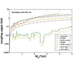
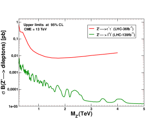
Figure 1: Left: Upper limit on the model parameters $x,y,z$. Right: 95% CL upper limits on the fiducial $Z^{\prime}$ production cross-section times the $Z^{\prime}\rightarrow\ell^{+}\ell^{-}$ branching [22] (green continuous line) and the corresponding upper limits on the $Z^{\prime}$ decaying to $\tau\overline{\tau}$ pairs [23] (red continuous line).

As our model is non-universal, it has two possible sources of FCNC: the non-universal couplings of the $Z^{\prime}$ and the couplings of the SM fermions to two scalar doublets. Since the charges of the first two families are equal, we can ignore constraints from observables with flavor changes between quarks and leptons of the first two families, such as: $K^{0}$-$\bar{K}^{0}$-mixing, $\mu$-$e$ conversion, etc. In our case, one of the strongest constraints on the parameters comes from $B^{0}$-$\bar{B}^{0}$-mixing. Figure 1 shows the upper limits on the $y$ and $z$ parameters at a 95% confidence level.

In two Higgs doublet models, FCNC can be avoided if the mass matrix for SM fermions with the same electric charge and isospin is generated from a single Higgs doublet. As we show in the appendix C, if the right-handed SM fermion is a singlet under the gauge group and if each right-handed SM singlet fermion couples to only one Higgs doublet (there is no problem if the scalar doublet has non-zero couplings to several right-handed fermions.), then there are no FCNC for the scalar sector; this is the case in our model.

5 Analysis of Higgs-like resonant signals

Recently, several anomalies have been reported in searches of high-mass scalar resonances in proton-proton collisions at the LHC. The 2HDMs are the most straightforward extensions of the Standard Model that can explain these observations. Additionally, our model includes a scalar singlet $\sigma$ that gives mass to the $Z^{\prime}$. The Higgs mechanism requires at least two CP-odd bosons to provide mass to the $Z$ and the $Z^{\prime}$ and one charged scalar boson to give mass to the SM $W$ boson, which leaves us with three CP even scalar bosons, one CP-odd scalar boson and one charged scalar. Our analysis aims to determine the typical masses for these bosons in the best-motivated parameter space and compare them with the experimental anomalies reported in the literature. As explained in detail in the Appendix A, of the three neutral scalar fields in the interaction space, $h_{1}$, $h_{2}$, and $\xi$, we can obtain using a unitary transformation, the neutral states in the mass space, $H_{1}$, $H_{2}$, $H_{3}$. Great interest has generated an anomaly that can be explained by a light neutral scalar Higgs with a mass $M_{H1}\approx 95$ GeV [26] and a charged Higgs around $M_{C^{\pm}}\approx$ 130 GeV [27]. For the charged Higgs, in [28] a detailed analysis of the phenomenological implications of a new resonance with a three sigma significance was studied. On a mass basis, we will denote as $M_{A}$ the only CP-odd field that is not absorbed as a Goldstone boson. An excess of events was also found in channels involving the productions of SM gauge bosons, $\gamma\gamma$ and $Z\gamma$ (for further analysis, look in [29] and references therein). This analysis provides a good indication of new scalar resonances decaying into two photons with invariant masses of 95 GeV [30] and 152 GeV [29]. Other excesses over the expected value in the SM for dibosons are reported at 680 GeV [31], which are compatible with the excess in $\gamma\gamma$ and $b\bar{b}$ reported by the CMS collaboration [32]. A more complete review of these anomalies and additional references can be found at [33]. In this reference, they also mention an excess reported by the ATLAS collaboration that can be interpreted as a pseudoscalar with a mass of 650 GeV produced in association with a scalar with a mass of 450 GeV.

Recently, a deviation from the background-only expectation occurred for high scalar resonances with masses $(575,200)$ GeV and a local (global) significance of 3.5 (2.0) standard deviations, as reported by the ATLAS collaboration [34]. It is important to stress that this analysis shows good agreement with the background-only hypothesis for the masses $(650,90)$ GeV, where CMS reported an excess with a local (global) significance of 3.8 (2.8) standard deviations [32].

To account for these experimental anomalies from the scalar potential of our model (see equation 32), we consider two possible assignments for the charges of the scalar singlet $\sigma$. One of them leads to a cubic coupling among the scalar fields, while the other to quartic term (the remaining terms in the scalar potential 32 are always present regardless of the $\sigma$ charge). If the $Z^{\prime}$ coupling of $\sigma$ is $x-y$, that is, $\alpha_{\sigma}=\alpha_{\nu 3}-\alpha_{\nu 1}$, then the following term is allowed:

$$\mu\left[(\Phi_{1}^{\dagger}\Phi_{2})\sigma+\text{h.c.}\right]\ .$$

In this case, the coupling constant $\mu$ has dimensions of mass, and in order to have a consistent mass spectrum, its values must be in the range $-77.3\leavevmode\nobreak\ \text{GeV}\leq\mu<0$. Similarly, if the coupling of $\sigma$ to the $Z^{\prime}$ boson is $\frac{1}{2}(x-y)$, or equivalently $\alpha_{\sigma}=(\alpha_{\nu 3}-\alpha_{\nu 1})/2$, it is possible to form the term

$$\lambda\left[(\Phi_{1}^{\dagger}\Phi_{2})\sigma^{2}+\text{h.c.})\right],$$ (28)

where the constant $\lambda$ is dimensionless, and restricted to the range $(-0.44,0)$. According to our scalar sector (whose scalar potential we show in Appendix A), to reproduce part of the spectrum of anomalies in the scalar sector (determined by the VEVs and coupling constants) we must identify the middle-mass neutral scalar boson as the SM Higgs boson to which we assign its well-known mass of $M_{H_{2}}=125$ GeV. In our model, we ensure that only the massive charged scalar field coincides with the anomaly $M_{C^{\pm}}=130$ GeV. This happens while the SM vector boson $W$ absorbs the other massless-charged field through the Higgs mechanism. Similarly, the Higgs mechanism requires a pseudoscalar field from one of the scalar doublets to give mass to the $Z$ boson, and the pseudoscalar field of the scalar singlet to give mass to the $Z^{\prime}$. The mass of the remaining scalar fields ($M_{H_{1}}$, $M_{H_{3}}$ and $M_{A}$) are free parameters. For the other dimensionless parameters of the potential (32), their values are assumed to be in the range $[-1.5,1.5]$. Regarding the VEVs of the $\Phi_{1}$ and $\Phi_{2}$, they are chosen such that $v_{1}^{2}+v_{2}^{2}=(246.24\leavevmode\nobreak\ \text{GeV})^{2}$ with $v_{2}\gg v_{1}$. This hierarchy between VEVs is necessary to align the Higgs doublet $\Phi_{2}$ with that of the SM. We take the VEV of the scalar singlet $\langle\sigma\rangle=v_{\sigma}/\sqrt{2}$ as a free parameter varying between 250 GeV and 2000 GeV. Finally, in order to satisfy the collider constraints, we require $z,y\ll x$, and take $x\gtrsim 1$ for $Z^{\prime}$ masses above $2$ TeV, as explained in section B.

To illustrate the density of solutions, Figures 2 and 3 display a total of 640 solutions spread across the $M_{H_{1}}$ vs $M_{H_{3}}$ and $M_{H_{1}}$ vs $M_{A}$ axes. It is important to emphasize our identification of the lightest CP-even Higgs scalar $H_{1}$ with the anomaly at 95 GeV. Therefore, we have considered exploring the mass interval 95 $\pm$ 10 GeV. In these figures, we can see that many of the experimental anomalies coincide with the regions with the highest density of solutions. This coincidence is important since we have made the free parameters of the theory vary in intervals that we consider natural.

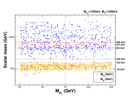
Figure 2: Distribution of the scalar mass $M_{H_{3}}$ (the blue round points) and the pseudoscalar $M_{A}$ (orange triangle points) for a scalar potential including the cubic term $\mu\Phi_{1}^{\dagger}\Phi_{2}\sigma+\text{h.c.}$. In this term, $\mu$ has mass dimensions and takes values in the range $(-77.3,0)$ GeV. We vary the other dimensionless parameters of the scalar potential in the range $[-1.5,1.5]$, and take the VEV of the scalar singlet $v_{\sigma}$ as a free parameter ranging from 250 to 2000 GeV. The VEV’s $v_{1}$ and $v_{2}$ vary subject to the conditions $\sqrt{v_{1}^{2}+v_{2}^{2}}=v=246.24\leavevmode\nobreak\ \text{GeV}$ and $v_{2}\gg v_{1}$. The masses of the scalars and pseudoscalars: $M_{H_{1}}$, $M_{H_{3}}$ and $M_{A}$ are determined by the tadpole equations (33). See the text for further details (see appendix A).

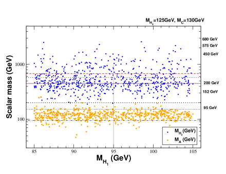
Figure 3: Distribution of the scalar mass $M_{H_{3}}$ (the blue round points) and the pseu-doscalar $M_{A}$ (orange triangle points) for a scalar potential including the quartic term $\lambda\Phi_{1}^{\dagger}\Phi_{2}\sigma^{2}+\text{h.c.}$. In this term, $\lambda$ is dimensionless and takes values in the interval $(-0.44,0)$. We vary the other dimensionless parameters of the scalar potential in the range $[-1.5,1.5]$, and take the VEV of the scalar singlet $v_{\sigma}$ as a free parameter ranging from 250 to 2000 GeV. The VEV’s $v_{1}$ and $v_{2}$ vary subject to the conditions $\sqrt{v_{1}^{2}+v_{2}^{2}}=v=246.24\leavevmode\nobreak\ \text{GeV}$ and $v_{2}\gg v_{1}$. The masses of the scalars and pseudoscalars: $M_{H_{1}}$, $M_{H_{3}}$ and $M_{A}$ are determined by the tadpole equations (33). See the text for further details.

6 Conclusions

In this work, we assume that the SM is a low energy effective theory of a more fundamental theory characterized by a gauge symmetry of the form $SU(3)_{\text{C}}\otimes SU(2)_{L}\otimes U(1)_{\alpha}\otimes U(1)_{\beta}$, and whose particle content is that of the SM extended with three right-handed neutrinos, a second Higgs doublet and a scalar singlet. Additionally, we impose that both $U(1)$ charges are non-universal and contribute non-trivially to the SM hypercharge, i.e., they are not inert charges. Under these assumptions, we showed that the most general expression for the $Z^{\prime}$ chiral couplings is as those shown in Table (3). In this model, it is possible to generate all the mass matrix elements of with only two Higgs doublets. From this, it is possible to adjust the model to reproduce the CKM and PMNS mixing matrices. This feature is highly non-trivial for non-universal scenarios and represents a great advantage of this model. It is important to mention that to maintain the non-universality condition, it was preferable to avoid Majorana mass terms (in our model, the constraints on the $U(1)$ charges arising from the Majorana mass terms, in the vast majority of cases, tend to generate universality). So, in our model, there is a link between Majorana masses and Universality.

From the assumptions of our work, as well as the collider, electroweak and flavor constraints, we also conclude that for a model with two non-inert Abelian symmetries at low energies ($M_{Z^{\prime}}<5$ TeV), only the residual symmetry $T_{3R}(3)$, in addition to the SM gauge symmetry, has an unsuppressed coupling strength. The argument $``3"$ says that only couplings to the third family are possible. Models with couplings to the first and second families are strongly constrained, so that only $Z^{\prime}$ couplings below 0.1 are possible, i.e., $g_{Z^{\prime}}\tilde{\epsilon}_{L,R}<0.1$. For a $Z^{\prime}$ coupling to the third family, it is possible to have $Z^{\prime}$ charges such that $g_{Z^{\prime}}\tilde{\epsilon}_{L,R}\sim 1$ for $Z^{\prime}$ masses above 2 TeV.

Our work analyzes some Higgs-like anomalies recently reported by the ATLAS and CMS collaborations [29]. To this end, we show the distribution of 400 solutions in the $M_{H_{1}}$, $M_{H_{3}}$ and $M_{H_{1}}$, $M_{A}$ planes. These results are shown in Figures 2 and 3. This analysis concludes that explaining some of the observed anomalies within the model is possible.

We show that the scalar sector FCNC cancel if each right-handed fermion couples only to a single Higgs doublet (although the scalar doublet can have non-zero couplings with several right-handed fermions). This will be the case as long as the right-handed fermions are singlets of the gauge group.

Appendices

Appendix A Scalar potential 

Our model contains two scalar doublets, $\Phi_{1}$ and $\Phi_{2}$, and a scalar singlet $\sigma$. In general, these fields can be expressed as

$$\Phi_{1}=\begin{pmatrix}\phi_{1}^{+}\\ \frac{v_{1}+h_{1}+i\,\eta_{1}}{\sqrt{2}}\end{pmatrix},\hskip 28.45274pt\Phi_{2}=\begin{pmatrix}\phi_{2}^{+}\\ \frac{v_{2}+h_{2}+i\,\eta_{2}}{\sqrt{2}}\end{pmatrix},\hskip 28.45274pt\sigma=\frac{v_{\sigma}+\xi+i\,\zeta}{\sqrt{2}}\ ,$$ (29)

where $\langle\Phi_{1}\rangle=(0,v_{1}/\sqrt{2})^{T}$, $\langle\Phi_{2}\rangle=(0,v_{2}/\sqrt{2})^{T}$ and $v_{\sigma}=\sqrt{2}\langle\sigma\rangle$. For the doublet $\Phi_{2}$ (which is close to $H_{1}$ in the Georgi basis) to be aligned with the Higgs of the SM we impose the hierarchy

$$v_{\sigma}>v_{2}\gg v_{1}\ .$$ (30)

Since the Higgs doublet is a linear combination of the two scalar doublets, then

$$\sqrt{v_{1}^{2}+v_{2}^{2}}=v=246.24\leavevmode\nobreak\ \text{GeV}\ ,$$ (31)

The most general scalar potential consistent with the gauge symmetry $SU(2)_{L}\otimes U(1)_{\alpha}\otimes U(1)_{\beta}$ is [30]:

$$\begin{split}V(\Phi_{1},\Phi_{2},\sigma)&=\mu_{1}^{2}\,|\Phi_{1}|^{2}+\mu_{2}^{2}\,|\Phi_{2}|^{2}+\mu_{\sigma}^{2}\,|\sigma|^{2}+\lambda_{1}\,|\Phi_{1}|^{4}+\lambda_{2}\,|\Phi_{2}|^{4}+\lambda_{\sigma}\,|\sigma|^{4}\\ &+\lambda_{3}\,|\Phi_{1}|^{2}|\Phi_{2}|^{2}+\lambda_{4}\,|\Phi_{1}^{\dagger}\Phi_{2}|^{2}+\lambda_{1\sigma}\,|\Phi_{1}|^{2}|\sigma|^{2}+\lambda_{2\sigma}\,|\Phi_{2}|^{2}|\sigma|^{2}\\ &+\text{linear term in }\sigma\ (\text{or quadratic term in }\sigma)\ ,\end{split}$$ (32)

where a linear interaction term in $\sigma$ (which we will denote as the cubic term) of the form

$$\mu\left[(\Phi_{1}^{\dagger}\Phi_{2})\sigma+\text{h.c.}\right]$$

is possible if $\alpha_{\sigma}$ in Table 2 is taken to be $\alpha_{\nu 3}-\alpha_{\nu 1}$. Here $\mu$ is a coupling with mass dimensions. On the other hand, if $\alpha_{\sigma}$ is equal to $\frac{1}{2}(\alpha_{\nu 3}-\alpha_{\nu 1})$, then the quadratic term in $\sigma$ (which we will denote as the quartic term),

$$\lambda\left[(\Phi_{1}^{\dagger}\Phi_{2})\sigma^{2}+\text{h.c.})\right]\ ,$$

is the one that is present. In this case, the coupling $\lambda$ is dimensionless. By minimizing the potential in Eq. (32), we then obtain that

$$\begin{split}\mu_{1}^{2}&=-\frac{\sqrt{2}}{2}\frac{\mu v_{2}v_{\sigma}}{v_{1}}-\lambda_{1}v_{1}^{2}-\frac{\lambda_{3}+\lambda_{4}}{2}v_{2}^{2}-\frac{\lambda_{1\sigma}}{2}v_{\sigma}^{2}\ ,\\ \mu_{2}^{2}&=-\frac{\sqrt{2}}{2}\frac{\mu v_{1}v_{\sigma}}{v_{2}}-\lambda_{2}v_{2}^{2}-\frac{\lambda_{3}+\lambda_{4}}{2}v_{1}^{2}-\frac{\lambda_{2\sigma}}{2}v_{\sigma}^{2}\ ,\\ \mu_{\sigma}^{2}&=-\frac{\sqrt{2}}{2}\frac{\mu v_{1}v_{2}}{v_{\sigma}}-\lambda_{\sigma}v_{\sigma}^{2}-\frac{\lambda_{1\sigma}}{2}v_{1}^{2}-\frac{\lambda_{2\sigma}}{2}v_{2}^{2}\ .\end{split}$$ (33)

in the cubic case, while in the quartic one, the corresponding expressions can be obtained from the previous ones by making the substitution $\sqrt{2}\mu\rightarrow\lambda v_{\sigma}$ .

A.1 Mass spectrum of the neutral scalar sector

From the potential (32) and the previous minimization conditions, we can build the mass matrices from the fields defined in Eq. (29). For the CP-even scalar field basis $(h_{1},h_{2},\xi)$, the mass matrix is given in the cubic case [35] by:

$$\begin{pmatrix}2\lambda_{1}v_{1}^{2}-\frac{\mu v_{2}v_{\sigma}}{\sqrt{2}v_{1}}&\frac{\mu v_{\sigma}}{\sqrt{2}}+v_{1}v_{2}(\lambda_{3}+\lambda_{4})&\frac{\mu v_{2}}{\sqrt{2}}+\lambda_{1\sigma}v_{1}v_{\sigma}\\ \frac{\mu v_{\sigma}}{\sqrt{2}}+v_{1}v_{2}(\lambda_{3}+\lambda_{4})&2\lambda_{2}v_{2}^{2}-\frac{\mu v_{1}v_{\sigma}}{\sqrt{2}v_{2}}&\frac{\mu v_{1}}{\sqrt{2}}+\lambda_{2\sigma}v_{2}v_{\sigma}\\ \frac{\mu v_{2}}{\sqrt{2}}+\lambda_{1\sigma}v_{1}v_{\sigma}&\frac{\mu v_{1}}{\sqrt{2}}+\lambda_{2\sigma}v_{2}v_{\sigma}&2\lambda_{\sigma}v_{\sigma}^{2}-\frac{\mu v_{1}v_{2}}{\sqrt{2}v_{\sigma}}\end{pmatrix},$$ (34)

while in the quartic case, it corresponds to:

$$\begin{pmatrix}2\lambda_{1}v_{1}^{2}-\frac{\lambda v_{2}v_{\sigma}^{2}}{2v_{1}}&\frac{\lambda v_{\sigma}^{2}}{2}+v_{1}v_{2}(\lambda_{3}+\lambda_{4})&v_{\sigma}(\lambda v_{2}+\lambda_{1\sigma}v_{1})\\ \frac{\lambda v_{\sigma}^{2}}{2}+v_{1}v_{2}(\lambda_{3}+\lambda_{4})&2\lambda_{2}v_{2}^{2}-\frac{\lambda v_{1}v_{\sigma}^{2}}{2v_{2}}&v_{\sigma}(\lambda v_{1}+\lambda_{2\sigma}v_{2})\\ v_{\sigma}(\lambda v_{2}+\lambda_{1\sigma}v_{1})&v_{\sigma}(\lambda v_{1}+\lambda_{2\sigma}v_{2})&2\lambda_{\sigma}v_{\sigma}^{2}\end{pmatrix}.$$ (35)

These are square mass matrices of rank three with mass eigenvalues $M_{H_{1}}$, $M_{H_{2}}$ and $M_{H_{3}}$, corresponding to the mass eigenstates $H_{1}$, $H_{2}$ and $H_{3}$, respectively. We will identify the states according to the mass hierarchy:

$$M_{H_{1}}<M_{H_{2}}<M_{H_{3}}\ .$$

The intermediate-mass scalar state, $H_{2}$, can be identified as the SM Higgs, while the light mass scalar state $H_{1}$ and the heavy mass scalar state $H_{3}$ are new scalar fields that, in principle, can be observed in the LHC experiments. The hierarchy (30) causes the scalar $H_{2}$ to align with $h_{2}$.

A.1.1 Mass spectrum of the neutral pseudoscalar sector

In the $(\eta_{1},\eta_{2},\zeta)$ basis, the pseudoscalar squared mass matrix takes the following form for the cubic case:

$$\frac{\mu}{\sqrt{2}}\begin{pmatrix}-\dfrac{v_{2}v_{\sigma}}{v_{1}}&v_{\sigma}&v_{2}\\ v_{\sigma}&-\dfrac{v_{1}v_{\sigma}}{v_{2}}&-v_{1}\\ v_{2}&-v_{1}&-\dfrac{v_{1}v_{2}}{v_{\sigma}}\end{pmatrix}.$$ (36)

The corresponding mass matrix for the quartic case is

$$\frac{\lambda v_{\sigma}}{2}\begin{pmatrix}-\dfrac{v_{2}v_{\sigma}}{v_{1}}&v_{\sigma}&2v_{2}\\ v_{\sigma}&-\dfrac{v_{1}v_{\sigma}}{v_{2}}&-2v_{1}\\ 2v_{2}&-2v_{1}&-4\dfrac{v_{1}v_{2}}{v_{\sigma}}\\ \end{pmatrix}.$$ (37)

In both cases, these mass matrices have rank 1. The two zero eigenvalues correspond to the two Goldstone bosons that give mass to the $Z$ and $Z^{\prime}$ bosons after the spontaneous symmetry breaking. The non-zero eigenvalue corresponds to a measurable pseudoscalar with mass equal to:

$$M^{2}_{A}=\begin{cases}-\dfrac{\mu\left(v_{1}^{2}v_{2}^{2}+v^{2}v_{\sigma}^{2}\right)}{\sqrt{2}v_{1}v_{2}v_{\sigma}}\,\,\,\,\,\,\,(\text{cubic case})\ ,\\ \\ -\dfrac{\lambda\left(4v_{1}^{2}v_{2}^{2}+v^{2}v_{\sigma}^{2}\right)}{2v_{1}v_{2}}\,\,\,\,(\text{quartic case})\ ,\end{cases}$$ (38)

whose mixing comes mainly from $\eta_{1}$.

A.1.2 Mass spectrum of the charged scalar sector

In the $(\phi_{1}^{\pm},\phi_{2}^{\pm})$ basis, the squared mass matrix for charged scalar particles is

$$\frac{1}{2}\begin{pmatrix}-\sqrt{2}\dfrac{\mu v_{2}v_{\sigma}}{v_{1}}-\lambda_{4}v^{2}_{2}&\sqrt{2}\mu v_{\sigma}+\lambda_{4}v_{1}v_{2}\\ \sqrt{2}\mu v_{\sigma}+\lambda_{4}v_{1}v_{2}&-\sqrt{2}\dfrac{\mu v_{1}v_{\sigma}}{v_{2}}-\lambda_{4}v^{2}_{1}\end{pmatrix},$$ (39)

for the cubic case, and

$$\frac{1}{2}\begin{pmatrix}-\dfrac{\lambda v_{2}v_{\sigma}^{2}}{v_{1}}-\lambda_{4}v_{2}&\lambda v_{\sigma}^{2}+\lambda_{4}v_{1}v_{2}\ \\ \lambda v_{\sigma}^{2}+\lambda_{4}v_{1}v_{2}&-\dfrac{\lambda v_{1}v_{\sigma}^{2}}{v_{2}}-\lambda_{4}v_{1}\end{pmatrix},$$ (40)

for the quartic case. As before, these mass matrices have rank 1, with the only zero eigenvalue corresponding to the Goldstone boson giving mass to the charged $W$ boson. The remaining charged scalar acquires a mass equal to

$$M^{2}_{C^{\pm}}=\begin{cases}-\dfrac{v^{2}}{2}\left(\sqrt{2}\dfrac{\mu v_{\sigma}}{v_{1}v_{2}}+\lambda_{4}\right)\ ,\,\,\,\,\,(\text{cubic case})\ ;\\ \\ -\dfrac{v^{2}}{2}\left(\dfrac{\lambda v_{\sigma}^{2}}{v_{1}v_{2}}+\lambda_{4}\right)\ ,\,\,\,\,\,\,\,\,\,\,\,\,(\text{quartic case})\ .\end{cases}$$ (41)

Appendix B The gauge boson masses

Let us now determine the mass of the neutral gauge bosons. These are obtained from the scalar-gauge couplings introduced by the covariant derivatives of the scalar fields in the Lagrangian terms

$$\mathcal{L}\supset|D_{\mu}\Phi_{1}|^{2}+|D_{\mu}\Phi_{2}|^{2}+|D_{\mu}\sigma|^{2}\ ,$$ (42)

where

$$D^{\mu}=\partial^{\mu}+\frac{i}{2}g_{L}A^{\mu}_{j}\hat{T}_{j}+\frac{i}{2}g_{\alpha}B^{\mu}_{\alpha}\hat{\alpha}+\frac{i}{2}g_{\beta}B^{\mu}_{\beta}\hat{\beta}\ ,$$ (43)

with $\hat{T}_{j}$, $A^{\mu}_{j}$ ($j=1,2,3$) and $g_{L}$ denoting, respectively, the generators, the gauge fields and the coupling constant associated with the weak isospin gauge group $SU(2)_{L}$, while $\hat{\chi}$, $B^{\mu}_{\chi}$ and $g_{\chi}$, with $\chi=\alpha,\beta$, are the corresponding quantities related with the two Abelian $U(1)$ factors. For the Higgs doublets $\Phi_{a}$ ($a=1,2$) and the singlet $\sigma$, we have

$$D^{\mu}\Phi_{a} =\left[\partial^{\mu}+\frac{i}{2}g_{L}\begin{pmatrix}A^{\mu}_{3}&\sqrt{2}W^{\mu}\\ \sqrt{2}W^{\mu\dagger}&-A^{\mu}_{3}\end{pmatrix}+\frac{i}{2}g_{\alpha}\alpha_{a}B^{\mu}_{\alpha}+\frac{i}{2}g_{\beta}\beta_{a}B^{\mu}_{\beta}\right]\Phi_{a}\ ,$$

$$D^{\mu}\sigma =\left(\partial^{\mu}+\frac{i}{2}g_{\alpha}\alpha_{\sigma}B^{\mu}_{\alpha}+\frac{i}{2}g_{\beta}\beta_{\sigma}B^{\mu}_{\beta}\right)\sigma\ ,$$ (44)

Here $\alpha_{a}$ ($\beta_{a}$) and $\alpha_{\sigma}$ ($\beta_{\sigma}$) denote, respectively, the $U(1)_{\alpha(\beta)}$ charges for $\Phi_{a}$ and $\sigma$ given in Tab. 2. Additionally, the $W$ field has been defined as

$$W^{\mu}=\dfrac{A^{\mu}_{1}-iA^{\mu}_{2}}{\sqrt{2}}\ .$$ (45)

Taking into account the definition of $\Phi_{a}$ and $\sigma$ given in Eq. (29), as well as the basis changes defined in Eqs. (6) and (7), which imply

$$B^{\mu}_{\chi} =a_{\chi}A^{\mu}+b_{\chi}Z^{\mu}+c_{\chi}Z^{\prime\mu}\ ,\ \ \ (\chi=\alpha,\beta)\ ;$$

$$A^{\mu}_{3} =\sin\theta_{W}A^{\mu}+\cos\theta_{W}Z^{\mu}\ ,$$ (46)

with

$$a_{\alpha} =\cos\theta\cos\theta_{W}\ ,\ \ \ b_{\alpha}=-\cos\theta\sin\theta_{W}\ ,\ \ \ c_{\alpha}=-\sin\theta\ ,$$

$$a_{\beta} =\sin\theta\cos\theta_{W}\ ,\ \ \ b_{\beta}=-\sin\theta\sin\theta_{W}\ ,\ \ \ \ c_{\beta}=\cos\theta\ ,$$ (47)

it can be shown that the mass terms for the $Z^{\mu}$, $Z^{\prime\mu}$ and $W^{\mu}$ gauge bosons are

$$\mathcal{L}\supset \frac{1}{2}\left(g^{2}_{Z}v^{2}\right)Z_{\mu}Z^{\mu}+\frac{1}{2}\left[g^{2}_{Z^{\prime}}\left(\gamma^{\prime 2}_{1}v^{2}_{1}+\gamma^{\prime 2}_{2}v^{2}_{2}+\gamma^{\prime 2}_{\sigma}v^{2}_{\sigma}\right)\right]Z^{\prime}_{\mu}Z^{\prime\mu}$$

$$-\frac{1}{2}\left[2g_{Z}g_{Z^{\prime}}\left(\gamma^{\prime}_{1}v^{2}_{1}+\gamma^{\prime}_{2}v^{2}_{2}\right)\right]Z_{\mu}Z^{\prime\mu}+g^{2}_{W}v^{2}W^{\dagger}_{\mu}W^{\mu},$$ (48)

the coupling constants $g_{Z}$ and $g_{W}$ are defined as in the SM, i.e.,

$$g_{Z}=\frac{g_{L}}{2\cos\theta_{W}}\ ,\ \ \ g_{W}=\frac{g_{L}}{2}\ ,$$ (49)

while $g_{Z^{\prime}}$ is defined through the following relations:

$$g_{Z^{\prime}}\gamma^{\prime}_{a} =-\frac{1}{2}\left(g_{\alpha}\alpha_{a}\sin\theta-g_{\beta}\beta_{a}\cos\theta\right)\ ,\ \ \ (a=1,2.);$$

$$g_{Z^{\prime}}\gamma^{\prime}_{\sigma} =-\frac{1}{2}\left(g_{\alpha}\alpha_{\sigma}\sin\theta-g_{\beta}\beta_{\sigma}\cos\theta\right).$$ (50)

In terms of the $x$, $y$, $z$ and $w$ parameters defined in Eq. (27), these couplings can be expressed as

$$g_{Z^{\prime}}\gamma^{\prime}_{1}=z-y\ ,\ \ \ g_{Z^{\prime}}\gamma^{\prime}_{2}=z-x\ ,\ \ \ g_{Z^{\prime}}\gamma^{\prime}_{\sigma}=-w\ .$$ (51)

Writing the $Z-Z^{\prime}$ mixing matrix as

$$M^{2}_{Z-Z^{\prime}}=\begin{bmatrix}g^{2}_{Z}v^{2}&-g_{Z}g_{Z^{\prime}}\gamma^{\prime}_{a}v^{2}_{a}\\ -g_{Z}g_{Z^{\prime}}\gamma^{\prime}_{a}v^{2}_{a}&g^{2}_{Z^{\prime}}\left(\gamma^{\prime 2}_{a}v^{2}_{a}+\gamma^{\prime 2}_{\sigma}v^{2}_{\sigma}\right)\end{bmatrix}\equiv\begin{pmatrix}\mathcal{A}&-\mathcal{C}\\ -\mathcal{C}&\mathcal{B}\\ \end{pmatrix},$$ (52)

with a sum over the $a$ index implied, then the square masses of the physical neutral gauge bosons $Z_{1}$ and $Z_{2}$ are given by

$$m^{2}_{Z_{1,2}}=\frac{1}{2}\left[\mathcal{A}+\mathcal{B}\mp\sqrt{\left(\mathcal{A}-\mathcal{B}\right)^{2}+4\mathcal{C}^{2}}\right].$$ (53)

If $\mathcal{O}$ is the diagonalizing orthogonal matrix defining the mass basis, i.e.,

$$\begin{pmatrix}Z^{\mu}\\ Z^{\prime\mu}\end{pmatrix}=\mathcal{O}\begin{pmatrix}Z^{\mu}_{1}\\ Z^{\mu}_{2}\end{pmatrix}=\begin{pmatrix}\cos\Theta&-\sin\Theta\\ \sin\Theta&\cos\Theta\end{pmatrix}\begin{pmatrix}Z^{\mu}_{1}\\ Z^{\mu}_{2}\end{pmatrix},$$ (54)

then the mixing angle $\Theta$ can be determined from

$$\tan 2\Theta=\frac{2\mathcal{C}}{\mathcal{B}-\mathcal{A}}\ .$$ (55)

From this expression, it is possible to obtain

$$\Theta=\frac{1}{2}\arctan\left\{\frac{g_{L}}{2\cos\theta_{W}}\frac{\left[(z-y)v_{1}^{2}+(z-x)v_{2}^{2}\right]}{\left[(z-y)^{2}v_{1}^{2}+(z-x)^{2}v_{2}^{2}+w^{2}v_{\sigma}^{2}\right]-\frac{g_{L}^{2}v^{2}}{4\cos^{2}\theta_{W}}}\right\}\ .$$ (56)

To satisfy the current constraint on the mixing angle [24] it is necessary to keep this angle below $10^{-3}$, which is possible in two scenarios: 1) a light $Z^{\prime}$ mass, i.e., $M_{Z^{\prime}}\ll M_{Z}$ or a heavy $Z^{\prime}$ mass, i.e., $M_{Z^{\prime}}\gg M_{Z}$, which requires $x\gtrsim 1$, $z\sim y\ll 1$ and $v<v_{\sigma}$. In analyzing the scalar anomalies $w=x-y$ in the cubic case, or $w=\frac{x-y}{2}$ for a potential with quartic coupling term (as explained in appendix A). For that analysis, assuming a heavy $Z^{\prime}$ mass is more convenient.

Appendix C Analysis of scalar FCNCs

The Yukawa interactions are described by the general Lagrangian

$$-\mathcal{L}_{Y}={\bar{q}^{\prime}_{iL}}y^{ad}_{ij}\Phi_{a}d^{\prime}_{jR}+{\bar{q}^{\prime}_{iL}}y^{au}_{ij}\tilde{\Phi}_{a}u^{\prime}_{jR}+{\bar{l}^{\prime}_{iL}}y^{ae}_{ij}\Phi_{a}e^{\prime}_{jR}+{\bar{l}^{\prime}_{iL}}y^{a\nu}_{ij}\tilde{\Phi}_{a}\nu^{\prime}_{jR}+\text{h.c.}\ ,$$ (57)

with $i,j=1,2,3$, and $a=1,2$. Here

$$\Phi_{a}=\begin{pmatrix}\phi_{a}^{+}\\ \dfrac{v_{a}+h_{a}+i\eta_{a}}{\sqrt{2}}\end{pmatrix}\ ,\ \ \ \ \tilde{\Phi}_{a}=i\sigma_{2}\Phi^{*}_{a}\ .$$ (58)

According to the non-universal $U(1)$ charges, the Yukawa couplings present in our model are

$$-\mathcal{L}_{Y} ={\bar{q}^{\prime}_{iL}}y^{1d}_{ia}\Phi_{1}d^{\prime}_{aR}+{\bar{q}^{\prime}_{iL}}y^{1u}_{ia}\tilde{\Phi}_{1}u^{\prime}_{aR}+{\bar{l}^{\prime}_{iL}}y^{1e}_{ia}\Phi_{1}e^{\prime}_{aR}+{\bar{l}^{\prime}_{iL}}y^{1\nu}_{ia}\tilde{\Phi}_{1}\nu^{\prime}_{aR}$$

$$+{\bar{q}^{\prime}_{iL}}y^{2d}_{i3}\Phi_{2}d^{\prime}_{3R}+{\bar{q}^{\prime}_{iL}}y^{2u}_{i3}\tilde{\Phi}_{2}u^{\prime}_{3R}+{\bar{l}^{\prime}_{iL}}y^{2e}_{i3}\Phi_{2}e^{\prime}_{3R}+{\bar{l}^{\prime}_{iL}}y^{2\nu}_{i3}\tilde{\Phi}_{2}\nu^{\prime}_{3R}+\text{h.c.}\ .$$ (59)

So, the Yukawa matrices have the following structure

$$Y^{1f}=\begin{pmatrix}y^{1f}_{11}&y^{1f}_{12}&0\\ y^{1f}_{21}&y^{1f}_{22}&0\\ y^{1f}_{31}&y^{1f}_{32}&0\end{pmatrix},\ \ \ \ Y^{2f}=\begin{pmatrix}0&0&y^{2f}_{13}\\ 0&0&y^{2f}_{23}\\ 0&0&y^{2f}_{33}\end{pmatrix}\ .$$ (60)

To analyze the FCNC, it is convenient to rotate the scalar doublets to the Giorgi basis where only one of the CP neutral even components of the doublets acquires VEV while the remaining ones are zero. Explicitly this corresponds to

$$\begin{pmatrix}\mathcal{H}_{1}\\ \mathcal{H}_{2}\end{pmatrix}=\begin{pmatrix}\cos\beta&\sin\beta\\ -\sin\beta&\cos\beta\end{pmatrix}\begin{pmatrix}\Phi_{1}\\ \Phi_{2}\end{pmatrix}\rightarrow\mathcal{H}_{\alpha}=R_{\alpha\beta}\Phi_{\beta}\ .$$ (61)

In the unitary gauge

$$\mathcal{H}_{1}=\begin{pmatrix}0\\ \dfrac{v+h}{\sqrt{2}}\end{pmatrix},\ \ \ \ \mathcal{H}_{2}=\begin{pmatrix}\mathcal{H}^{+}\\ \dfrac{\mathcal{H}^{0}+i\mathcal{A}^{0}}{\sqrt{2}}\end{pmatrix}\ .$$ (62)

The Georgi basis should not be confused with the mass states of the scalar bosons. As discussed in Ref. [36], in this basis, the $\mathcal{H}_{1}$ boson gives mass to the SM fermions (the scalar singlet does not couple to SM fermions) and does not generate FCNC. Therefore, it is not convenient to use the mass eigenstates, a mixture of the scalar singlet and the doublets, when studying the interactions between the scalar sector and the SM fermions. In most observables, the scalar boson is a virtual particle, and the boson that interacts with the SM fermions is the projection onto the subspace formed by the two doublets. In 2HDM, this feature is very useful since FCNC in the scalar sector can only be generated by $\mathcal{H}_{2}$. Therefore, in this work, we focus on the CP-even neutral component of this doublet.

In terms of the new basis,

$$y^{\alpha f}_{ij}\Phi_{\alpha} =x^{\alpha f}_{ij}\mathcal{H}_{\alpha}\ ,$$

$$y^{\alpha f}_{ij}\tilde{\Phi}_{\alpha} =x^{\alpha f}_{ij}\tilde{\mathcal{H}}_{\alpha}\ ,$$ (63)

the rotated yukawa couplings are

$$x^{1f}_{ij} =\cos\beta\ y^{1f}_{ij}+\sin\beta\ y^{2f}_{ij}\ ,$$

$$x^{2f}_{ij} =-\sin\beta\ y^{1f}_{ij}+\cos\beta\ y^{2f}_{ij}\ .$$ (64)

Thus

$$\mathcal{L}_{Y}= -{\bar{q}^{\prime}_{iL}}x^{\alpha d}_{ij}\mathcal{H}_{\alpha}d^{\prime}_{jR}-{\bar{q}^{\prime}_{iL}}x^{\alpha u}_{ij}\tilde{\mathcal{H}}_{\alpha}u^{\prime}_{jR}-{\bar{l}^{\prime}_{iL}}x^{\alpha e}_{ij}\mathcal{H}_{\alpha}e^{\prime}_{jR}-{\bar{l}^{\prime}_{iL}}x^{\alpha\nu}_{ij}\tilde{\mathcal{H}}_{\alpha}\nu^{\prime}_{jR}+h.c.\ ,$$

$$= -{\bar{q}^{\prime}_{iL}}x^{1d}_{ij}\mathcal{H}_{1}d^{\prime}_{jR}-{\bar{q}^{\prime}_{iL}}x^{2d}_{ij}\mathcal{H}_{2}d^{\prime}_{jR}-{\bar{q}^{\prime}_{iL}}x^{1u}_{ij}\tilde{\mathcal{H}}_{1}u^{\prime}_{jR}-{\bar{q}^{\prime}_{iL}}x^{2u}_{ij}\tilde{\mathcal{H}}_{2}u^{\prime}_{jR}$$

$$-{\bar{l}^{\prime}_{iL}}x^{1e}_{ij}\mathcal{H}_{1}e^{\prime}_{jR}-{\bar{l}^{\prime}_{iL}}x^{2e}_{ij}\mathcal{H}_{2}e^{\prime}_{jR}-{\bar{l}^{\prime}_{iL}}x^{1\nu}_{ij}\tilde{\mathcal{H}}_{1}\nu^{\prime}_{jR}-{\bar{l}^{\prime}_{iL}}x^{2\nu}_{ij}\tilde{\mathcal{H}}_{2}\nu^{\prime}_{jR}+h.c.\ ,$$

$$= -\frac{1}{\sqrt{2}}\left(v+h\right)\left({\bar{d}^{\prime}_{iL}}x^{1d}_{ij}d^{\prime}_{jR}+{\bar{u}^{\prime}_{iL}}x^{1u}_{ij}u^{\prime}_{jR}+{\bar{e}^{\prime}_{iL}}x^{1e}_{ij}e^{\prime}_{jR}+{\bar{\nu}^{\prime}_{iL}}x^{1\nu}_{ij}\nu^{\prime}_{jR}\right)$$

$$-\frac{1}{\sqrt{2}}\left(\mathcal{H}^{0}+i\mathcal{A}^{0}\right)\left({\bar{d}^{\prime}_{iL}}x^{2d}_{ij}d^{\prime}_{jR}+{\bar{e}^{\prime}_{iL}}x^{2e}_{ij}e^{\prime}_{jR}\right)-\frac{1}{\sqrt{2}}\left(\mathcal{H}^{0}-i\mathcal{A}^{0}\right)\left({\bar{u}^{\prime}_{iL}}x^{2u}_{ij}u^{\prime}_{jR}+{\bar{\nu}^{\prime}_{iL}}x^{2\nu}_{ij}\nu^{\prime}_{jR}\right)$$

$$-\mathcal{H}^{+}\left({\bar{u}^{\prime}_{iL}}x^{2d}_{ij}d^{\prime}_{jR}+{\bar{\nu}^{\prime}_{iL}}x^{2e}_{ij}e^{\prime}_{jR}\right)+\mathcal{H}^{-}\left({\bar{d}^{\prime}_{iL}}x^{2u}_{ij}u^{\prime}_{jR}+{\bar{e}^{\prime}_{iL}}x^{2\nu}_{ij}\nu^{\prime}_{jR}\right)+h.c.\ ,$$

where we have taken into account that $\tilde{\mathcal{H}}_{2}=\left(\frac{\mathcal{H}^{0}-i\mathcal{A}^{0}}{\sqrt{2}},-\mathcal{H}^{-}\right)^{T}$. Next, we define the fermion mass eigenstates as:

$$f_{L}\equiv V^{f\dagger}_{L}f^{\prime}_{L}\ ,\ \ \ f_{R}\equiv V^{f\dagger}_{R}f^{\prime}_{R}\ ,$$ (65)

with $V^{f}_{L(R)}$ are appropriated unitary matrices. In terms of the non-prime fields, we get

$$\mathcal{L}_{Y}= -\frac{1}{\sqrt{2}}\left(v+h\right)\left({\bar{d}_{iL}}z^{1d}_{ij}d_{jR}+{\bar{e}_{iL}}z^{1e}_{ij}e_{jR}+{\bar{u}_{iL}}z^{1u}_{ij}u_{jR}+{\bar{\nu}_{iL}}z^{1\nu}_{ij}\nu_{jR}\right)$$

$$-\frac{1}{\sqrt{2}}\left(\mathcal{H}^{0}+i\mathcal{A}^{0}\right)\left({\bar{d}_{iL}}z^{2d}_{ij}d_{jR}+{\bar{e}_{iL}}z^{2e}_{ij}e_{jR}\right)-\frac{1}{\sqrt{2}}\left(\mathcal{H}^{0}-i\mathcal{A}^{0}\right)\left({\bar{u}_{iL}}z^{2u}_{ij}u_{jR}+{\bar{\nu}_{iL}}z^{2\nu}_{ij}\nu_{jR}\right)$$

$$-\mathcal{H}^{+}\left({\bar{u}_{iL}}z^{2ud}_{ij}d_{jR}+{\bar{\nu}_{iL}}z^{2\nu e}_{ij}e_{jR}\right)+\mathcal{H}^{-}\left({\bar{d}_{iL}}z^{2du}_{ij}u_{jR}+{\bar{e}_{iL}}z^{2e\nu}_{ij}\nu_{jR}\right)+h.c.\ ,$$ (66)

where

$$z^{\alpha f}\equiv V^{f\dagger}_{L}x^{\alpha f}V^{f}_{R}\ ,\ \ \ \ z^{2gf}\equiv V^{g\dagger}_{L}x^{2f}V^{f}_{R}\ .$$ (67)

In this way, from Eqs. (64), we get

$$z^{1f}= \cos\beta\left(V^{f\dagger}_{L}y^{1f}V^{f}_{R}\right)+\sin\beta\left(V^{f\dagger}_{L}y^{2f}V^{f}_{R}\right)\ ,$$ (68)

$$z^{2f}= -\sin\beta\left(V^{f\dagger}_{L}y^{1f}V^{f}_{R}\right)+\cos\beta\left(V^{f\dagger}_{L}y^{2f}V^{f}_{R}\right)\ ,$$ (69)

$$z^{2gf}= -\sin\beta\left(V^{g\dagger}_{L}y^{1f}V^{f}_{R}\right)+\cos\beta\left(V^{g\dagger}_{L}y^{2f}V^{f}_{R}\right)\ .$$ (70)

In the Georgi basis, only the CP-odd component of $\mathcal{H}_{1}$ acquires VEV, and therefore, the interaction of the SM fermions with this doublet generates the masses of quarks and leptons; consequently, in the mass eigenstates the matrix $z^{1f}$ must be diagonal, i.e.,

$$z^{1f}=\begin{pmatrix}\frac{\sqrt{2}m^{f}_{1}}{v}&0&0\\ 0&\frac{\sqrt{2}m^{f}_{2}}{v}&0\\ 0&0&\frac{\sqrt{2}m^{f}_{3}}{v}\\ \end{pmatrix},$$ (71)

where $m^{f}_{i}$ corresponds to the mass of the fermion $f_{i}$. Because in our model, the right-handed quarks and leptons are singlets under the gauge group we can define the right-handed fermions as: $f_{j}^{\prime\prime}=\left(V^{f}_{R}\right)_{ij}f_{j}$ for all $f$, such that $V^{f}_{R}$ completely disappears from the Lagrangian. This transformation leaves all the terms invariant under the gauge group since the gauge singlets are of the form $\bar{f}_{Ri}f_{i}$ or $\bar{f}_{Ri}\partial_{\mu}f_{i}$ and $V^{f}_{R}$ is a global transformation. We are not modifying the Yukawa interaction terms since we are only redefining them. In this way, the coupling of fermions to scalar bosons is

$$z^{\alpha f}\equiv V^{f\dagger}_{L}x^{\alpha f}V^{f}_{R}\rightarrow V^{f\dagger}_{L}x^{\alpha f}.$$

A consequence of this result is that if the Yukawa coupling of a scalar boson to one of the right-handed fermions is zero in the interaction space, i.e., $y^{\alpha f}_{ij}=0$ for all $j$, then in mass eigenstates, the corresponding Yukawa coupling is also identically zero, i.e., $V^{f}_{ik}y^{\alpha f}_{kj}=0$ for all $j$. That is, if the diagonalization matrix $V^{f}_{L}$ of the left-handed fermions $f$ is given by

$$V^{f}_{L}=\begin{pmatrix}v^{f}_{11}&v^{f}_{12}&v^{f}_{13}\\ v^{f}_{21}&v^{f}_{22}&v^{f}_{23}\\ v^{f}_{31}&v^{f}_{32}&v^{f}_{33}\end{pmatrix},$$ (72)

the Eq. (60) implies that

$$V^{f\dagger}_{L}y^{1f}= \begin{pmatrix}v^{*}_{11}y^{1f}_{11}+v^{*}_{21}y^{1f}_{21}+v^{*}_{31}y^{1f}_{31}&v^{*}_{11}y^{1f}_{12}+v^{*}_{21}y^{1f}_{22}+v^{*}_{31}y^{1f}_{32}&0\\ v^{*}_{12}y^{1f}_{11}+v^{*}_{22}y^{1f}_{21}+v^{*}_{32}y^{1f}_{31}&v^{*}_{12}y^{1f}_{12}+v^{*}_{22}y^{1f}_{22}+v^{*}_{32}y^{1f}_{32}&0\\ v^{*}_{13}y^{1f}_{11}+v^{*}_{23}y^{1f}_{21}+v^{*}_{33}y^{1f}_{31}&v^{*}_{13}y^{1f}_{12}+v^{*}_{23}y^{1f}_{22}+v^{*}_{33}y^{1f}_{32}&0\end{pmatrix}\ ,$$

$$V^{f\dagger}_{L}y^{2f}= \begin{pmatrix}0&0&v^{*}_{11}y^{2f}_{13}+v^{*}_{21}y^{2f}_{23}+v^{*}_{31}y^{2f}_{33}\\ 0&0&v^{*}_{12}y^{2f}_{13}+v^{*}_{22}y^{2f}_{23}+v^{*}_{32}y^{2f}_{33}\\ 0&0&v^{*}_{13}y^{2f}_{13}+v^{*}_{23}y^{2f}_{23}+v^{*}_{33}y^{2f}_{33}\end{pmatrix}.$$ (73)

Since the coupling $z^{1f}$ is diagonal, from the relation $z^{1f}=\cos\beta V^{f\dagger}_{L}y^{1f}+\sin\beta V^{f\dagger}_{L}y^{2f}$ and from the fact that if $\left(V^{f}_{L}y^{1f}\right)_{ij}=0$ then $\left(V^{f}_{L}y^{2f}\right)_{ij}\neq 0$ and the opposite, it must be true that each of the contributions must be diagonal. From the expressions (73) we have

$$z^{1f}_{ij}= z^{1f}_{i}\delta_{ij}=\cos\beta\left(V^{f}_{L}y^{1f}\right)_{ij},\hskip 14.22636pt\text{for any $i$ and $j=1,2$}\ .$$

$$z^{1f}_{ij}= z^{1f}_{i}\delta_{ij}=\sin\beta\left(V^{f}_{L}y^{2f}\right)_{ij},\hskip 14.22636pt\text{for any $i$ and $j=3$}\ .$$ (74)

That is to say, $\left(V^{f}_{L}y^{1f}\right)_{ij}$ and $\left(V^{f}_{L}y^{2f}\right)_{ij}$ are diagonal matrix with $\left(V^{f}_{L}y^{1f}\right)_{33}=0$ and $\left(V^{f}_{L}y^{2f}\right)_{11}=\left(V^{f}_{L}y^{2f}\right)_{22}=0$. From these results, the Yukawa couplings of $\mathcal{H}_{2}$ with the physical fermions turn out to be diagonal:

$$z^{2f}=-\sin\beta\left(V^{f}_{L}y^{1f}\right)_{ij}+\cos\beta\left(V^{f}_{L}y^{2f}\right)_{ij}=-\tan\beta z_{i}^{1f}\delta_{ij}|_{i,j\in(1,2)}+\cot\beta z_{i}^{1f}\delta_{i3}\ .$$

In the last step we obtained the expressions for $\left(V^{f}_{L}y^{1f}\right)_{ij}$ and $\left(V^{f}_{L}y^{2f}\right)_{ij}$ from Eq. (74). In matrix form this result can be written as

$$z^{2f}=\begin{pmatrix}-\tan\beta z_{1}^{1f}&0&0\\ 0&-\tan\beta z_{2}^{1f}&0\\ 0&0&\cot\beta z^{1f}_{3}\end{pmatrix}\ .$$ (75)

This result is important because it shows that the coupling of the neutral scalars in the mass eigenstates of the SM fermions is diagonal. Therefore, our model does not present FCNC in the scalar sector. In most cases, the exact values of the matrix $y^{\alpha f}_{ij}$ are entirely unknown, and what we know are the diagonal couplings, $z_{i}=\frac{\sqrt{2}}{v}m_{i}^{f}$, where $m_{i}^{f}$ is a diagonal matrix whose elements correspond to the fermion masses in the SM. so that the Yukawa couplings will be given by

$$y^{1f}_{ij}= V^{f\dagger}_{Lik}\frac{\sqrt{2}}{v\cos\beta}m_{k}^{1f}\delta_{kj}\ ,\text{ where $m_{3}^{1f}=0$}\ .$$

Here $m^{1f}$ is a diagonal matrix with the first two eigenvalues equal to the masses of the particles in the SM and a third element equal to zero. We have a similar expression for the second term in (68)

$$y^{2f}_{ij}= V^{f\dagger}_{Lik}\frac{\sqrt{2}}{v\sin\beta}m_{k}^{2f}\delta_{kj}\ ,\text{ where $m_{1}^{2f}=m_{2}^{2f}=0$}\ .$$

Here $m^{2f}$ is a diagonal matrix with the first two eigenvalues equal to zero and a third element equal to the corresponding mass in the SM. On the other hand, the Yukawa couplings inducing flavor-changing charged currents can be written as shown below:

$$z^{2ud} =-\sin\beta\left[V^{u\dagger}_{L}V^{d}_{L}\left(V^{d\dagger}_{L}y^{1d}V^{d}_{R}\right)\right]+\cos\beta\left[V^{u\dagger}_{L}V^{d}_{L}\left(V^{d\dagger}_{L}y^{2d}V^{d}_{R}\right)\right]\ ,$$

$$z^{2du} =-\sin\beta\left[V^{d\dagger}_{L}V^{u}_{L}\left(V^{u\dagger}_{L}y^{1u}V^{u}_{R}\right)\right]+\cos\beta\left[V^{d\dagger}_{L}V^{u}_{L}\left(V^{u\dagger}_{L}y^{2u}V^{u}_{R}\right)\right]\ ,$$

$$z^{2\nu e} =-\sin\beta\left[V^{\nu\dagger}_{L}V^{e}_{L}\left(V^{e\dagger}_{L}y^{1e}V^{e}_{R}\right)\right]+\cos\beta\left[V^{\nu\dagger}_{L}V^{e}_{L}\left(V^{e\dagger}_{L}y^{2e}V^{e}_{R}\right)\right]\ ,$$

$$z^{2e\nu} =-\sin\beta\left[V^{e\dagger}_{L}V^{\nu}_{L}\left(V^{\nu\dagger}_{L}y^{1\nu}V^{\nu}_{R}\right)\right]+\cos\beta\left[V^{e\dagger}_{L}V^{\nu}_{L}\left(V^{\nu\dagger}_{L}y^{1\nu}V^{\nu}_{R}\right)\right]\ .$$

Remembering that $V_{\text{CKM}}=V^{u\dagger}_{L}V^{d}_{L}\equiv V$ and $V_{\text{PMNS}}=V^{e\dagger}_{L}V^{\nu}_{L}\equiv U$, it is easy to see from eq. (69) that

$$z^{2ud}=Vz^{2d}\ ,\ \ \ z^{2du}=V^{\dagger}z^{2u}\ ,\ \ \ z^{2\nu e}=U^{\dagger}z^{2e}\ ,\ \ \ z^{2e\nu}=Uz^{2\nu}\ .$$ (76)

References

• [1] John F. Donoghue, Eugene Golowich, and Barry R. Holstein. Dynamics of the Standard Model. Cambridge Monographs on Particle Physics, Nuclear Physics and Cosmology. Cambridge University Press, 2 edition, 2014.
• [2] Aleandro Nisati and Vivek Sharma, editors. Discovery of the Higgs Boson. World Scientific, Hackensack, 2017.
• [3] R. L. Workman et al. Review of Particle Physics. PTEP, 2022:083C01, 2022.
• [4] Georges Aad et al. Measurements of the Higgs boson production and decay rates and constraints on its couplings from a combined ATLAS and CMS analysis of the LHC pp collision data at $\sqrt{s}=7$ and 8 TeV. JHEP, 08:045, 2016.
• [5] Ernest Ma. Hierarchical Radiative Quark and Lepton Mass Matrices. Phys. Rev. Lett., 64:2866–2869, 1990.
• [6] Paul Langacker. Grand Unified Theories and Proton Decay. Phys. Rept., 72:185, 1981.
• [7] Michael Dine, Willy Fischler, and Mark Srednicki. A Simple Solution to the Strong CP Problem with a Harmless Axion. Phys. Lett. B, 104:199–202, 1981.
• [8] Richard H. Benavides, D. V. Forero, Luis Muñoz, Jose M. Muñoz, Alejandro Rico, and A. Tapia. Five texture zeros in the lepton sector and neutrino oscillations at DUNE. Phys. Rev. D, 107(3):036008, 2023.
• [9] R. Alonso, M. B. Gavela, G. Isidori, and L. Maiani. Neutrino Mixing and Masses from a Minimum Principle. JHEP, 11:187, 2013.
• [10] R. N. Mohapatra and A. Y. Smirnov. Neutrino Mass and New Physics. Ann. Rev. Nucl. Part. Sci., 56:569–628, 2006.
• [11] Saul Perlmutter. Supernovae, dark energy, and the accelerating universe: The Status of the cosmological parameters. Int. J. Mod. Phys. A, 15S1:715–739, 2000.
• [12] Austin Joyce, Bhuvnesh Jain, Justin Khoury, and Mark Trodden. Beyond the Cosmological Standard Model. Phys. Rept., 568:1–98, 2015.
• [13] E. Golowich and P. B. Pal. Charge quantization from anomalies. Phys. Rev. D, 41:3537–3540, 1990.
• [14] D. Decamp et al. Determination of the Number of Light Neutrino Species. Phys. Lett. B, 231:519–529, 1989.
• [15] John Ellis. Outstanding questions: Physics beyond the Standard Model. Phil. Trans. Roy. Soc. Lond. A, 370:818–830, 2012.
• [16] Salvatore Capozziello and Mariafelicia De Laurentis. Extended Theories of Gravity. Phys. Rept., 509:167–321, 2011.
• [17] Elcio Abdalla et al. Cosmology intertwined: A review of the particle physics, astrophysics, and cosmology associated with the cosmological tensions and anomalies. JHEAp, 34:49–211, 2022.
• [18] Jens Erler, Paul Langacker, Shoaib Munir, and Eduardo Rojas. Z’ Bosons at Colliders: a Bayesian Viewpoint. JHEP, 11:076, 2011.
• [19] Camilo Salazar, Richard H. Benavides, William A. Ponce, and Eduardo Rojas. LHC Constraints on 3-3-1 Models. JHEP, 07:096, 2015.
• [20] Eduardo Rojas and Jens Erler. Alternative Z’ bosons in E6. JHEP, 10:063, 2015.
• [21] Richard H. Benavides, Luis Muñoz, William A. Ponce, Oscar Rodríguez, and Eduardo Rojas. Electroweak couplings and LHC constraints on alternative Z’ models in $E_{6}$. Int. J. Mod. Phys. A, 33(35):1850206, 2018.
• [22] Georges Aad et al. Search for high-mass dilepton resonances using 139 fb-1 of $pp$ collision data collected at $\sqrt{s}=$13 TeV with the ATLAS detector. Phys. Lett. B, 796:68–87, 2019.
• [23] Morad Aaboud et al. Search for additional heavy neutral Higgs and gauge bosons in the ditau final state produced in 36 fb-1 of pp collisions at $\sqrt{s}=13$ TeV with the ATLAS detector. JHEP, 01:055, 2018.
• [24] Jens Erler, Paul Langacker, Shoaib Munir, and Eduardo Rojas. Improved Constraints on Z-prime Bosons from Electroweak Precision Data. JHEP, 08:017, 2009.
• [25] Jens Erler. Global fits to electroweak data using GAPP. In Physics at Run II: QCD and Weak Boson Physics Workshop: 2nd General Meeting, 6 1999.
• [26] Albert M Sirunyan et al. Search for a standard model-like Higgs boson in the mass range between 70 and 110 GeV in the diphoton final state in proton-proton collisions at $\sqrt{s}=$ 8 and 13 TeV. Phys. Lett. B, 793:320–347, 2019.
• [27] Georges Aad et al. Search for a light charged Higgs boson in $t\rightarrow H^{\pm}b$ decays, with $H^{\pm}\rightarrow cb$, in the lepton+jets final state in proton-proton collisions at $\sqrt{s}=13$ TeV with the ATLAS detector. JHEP, 09:004, 2023.
• [28] Abdesslam Arhrib, Mohamed Krab, and Souad Semlali. Accommodating the LHC Charged Higgs Boson Excess at 130 GeV in the General Two-Higgs Doublet Model. 2 2024.
• [29] Andreas Crivellin, Yaquan Fang, Oliver Fischer, Srimoy Bhattacharya, Mukesh Kumar, Elias Malwa, Bruce Mellado, Ntsoko Rapheeha, Xifeng Ruan, and Qiyu Sha. Accumulating evidence for the associated production of a new Higgs boson at the LHC. Phys. Rev. D, 108(11):115031, 2023.
• [30] Sumit Banik, Andreas Crivellin, Syuhei Iguro, and Teppei Kitahara. Asymmetric di-Higgs signals of the next-to-minimal 2HDM with a U(1) symmetry. Phys. Rev. D, 108(7):075011, 2023.
• [31] Albert M Sirunyan et al. Measurements of properties of the Higgs boson decaying into the four-lepton final state in pp collisions at $\sqrt{s}=13$ TeV. JHEP, 11:047, 2017.
• [32] Search for a new resonance decaying to two scalars in the final state with two bottom quarks and two photons in proton-proton collisions at $\sqrt{s}=13\,\mathrm{TeV}$. 2022.
• [33] Andreas Crivellin and Bruce Mellado. Anomalies in Particle Physics. 9 2023.
• [34] Georges Aad et al. Search for a resonance decaying into a scalar particle and a Higgs boson in the final state with two bottom quarks and two photons in proton-proton collisions at a center of mass energy of 13 TeV with the ATLAS detector. 4 2024.
• [35] William A. Ponce, Yithsbey Giraldo, and Luis A. Sanchez. Minimal scalar sector of 3-3-1 models without exotic electric charges. Phys. Rev. D, 67:075001, 2003.
• [36] Howard Georgi and Dimitri V. Nanopoulos. Suppression of Flavor Changing Effects From Neutral Spinless Meson Exchange in Gauge Theories. Phys. Lett. B, 82:95–96, 1979.