Transformations to simplify phylogenetic networks

Abstract

The evolutionary relationships between species are typically represented in the biological literature by rooted phylogenetic trees. However, a tree fails to capture ancestral reticulate processes, such as the formation of hybrid species or lateral gene transfer events between lineages, and so the history of life is more accurately described by a rooted phylogenetic network. Nevertheless, phylogenetic networks may be complex and difficult to interpret, so biologists sometimes prefer a tree that summarises the central tree-like trend of evolution. In this paper, we formally investigate methods for transforming an arbitrary phylogenetic network into a tree (on the same set of leaves) and ask which ones (if any) satisfy a simple consistency condition. This consistency condition states that if we add additional species into a phylogenetic network (without otherwise changing this original network) then transforming this enlarged network into a rooted phylogenetic tree induces the same tree on the original set of species as transforming the original network. We show that the LSA (lowest stable ancestor) tree method satisfies this consistency property, whereas several other commonly used methods (and a new one we introduce) do not. We also briefly consider transformations that convert arbitrary phylogenetic networks to another simpler class, namely normal networks.

June 2024

Keywords: phylogenetic networks, trees, transformations, lowest stable ancestor

1 Introduction

The traditional representation of evolutionary history is based on rooted phylogenetic trees. Such trees provide a simple illustration of speciation events and ancestry. The leaves correspond to known species, and the root represents the most recent common ancestor of this set of species. However, a tree fails to capture ancestral reticulate processes, such as hybridisation events or lateral gene transfer. Thus, the evolutionary history is more accurately described by rooted phylogenetic networks (Huson et al., , 2010; Steel, , 2016). Nevertheless, it is often helpful to extract the overall tree-like pattern that is present in a complex and highly reticulated network, sometimes referred to as the ‘central tree-like trend’ in the evolution of the taxa (Puigbò et al., , 2013; Wolf et al., , 2002). Such a tree is less complete than a network, but it is more easily interpreted and visualised (DeSalle and Riley, , 2020).

In this paper, we investigate ways to transform arbitrary rooted phylogenetic networks into rooted phylogenetic trees. There are many ways to do this, and we take an axiomatic approach, listing three desirable properties for such a transformation. We show that several current methods fail to satisfy all three properties; however, one transformation (the LSA tree construction) satisfies all three. Our approach is similar in spirit to an analogous axiomatic treatment of consensus methods (which transform an arbitrary set of trees into a single tree) in Bryant et al., (2017). We also briefly consider transformations that convert phylogenetic networks to ‘normal’ networks (a class of networks that allows a limited degree of reticulation). We begin by defining some concepts that will play a central role in our axiomatic approach.

1.1 Preliminaries

In this paper, we only consider rooted phylogenetic networks and trees. We let $\mathds{N}(X)$ denote the set of rooted phylogenetic networks, and $\mathds{T}(X)$ be the set of rooted phylogenetic trees on a leaf set $X$ of taxa. The labelled leaves are vertices of in-degree $1$ and out-degree $0$. The remaining interior vertices are unlabelled and of out-degree at least $1$.

In contrast to trees, we distinguish tree vertices with an in-degree of $1$ from reticulate vertices of an in-degree at least $1$ in phylogenetic networks. Following the definition of Huson et al., (2010), we assume that networks are bicombining. This means that each reticulate vertex has an in-degree of $2$ and an out-degree of $1$.

Consider a network $N\in\mathds{N}(X)$ and a subset $Y\subseteq X$. The network $N|Y$ is obtained from $N$ by restricting $N$ to the leaves in $Y$. When $|Y|=3$, the resulting network is called a trinet (Semple and Toft, , 2021). We say that a rooted tree with exactly three leaves is a rooted triple. In comparison to trinets, which can take an unlimited number of (unlabelled) shapes, there are only two distinct shapes for rooted triples (Steel, , 2016). The concept of rooted triples can be used to establish the isomorphism of two trees. The following result is classical and well known (for a proof, see, e.g. Theorem 1 from Bryant and Steel, (1995)).

Lemma 1.

Two phylogenetic trees $T,T^{\prime}\in\mathds{T}(X)$ are isomorphic if and only if, for every subset $U\subseteq X$ such that $|U|=3$, the trees $T$ restricted to $U$ and $T^{\prime}$ restricted to $U$ are isomorphic:

$$T\cong T^{\prime}\Longleftrightarrow T|U\cong T^{\prime}|U~{}\forall U\subseteq X:|U|=3.$$ (1.1)

We also require the following notion. Let $\Sigma_{X}$ denote the group of permutations on $X$. Given a network $N\in\mathds{N}(X)$ and a permutation $\sigma\in\Sigma_{X}$, let $N^{\sigma}$ denote the network obtained by reordering the labels of the leaves according to $\sigma$.

2 Axiomatic properties for transformations that simplify phylogenetic networks

Let $\mathds{N}^{\prime}(X)$ be a subclass of the set of all phylogenetic networks $\mathds{N}(X)$ on leaf set $X$, which satisfies the property $N\in\mathds{N}^{\prime}(X)$ and $\sigma\in\Sigma_{X}\Rightarrow N^{\sigma}\in\mathds{N}^{\prime}(X)$. Mainly, we focus on the case where $\mathds{N}^{\prime}(X)=\mathds{T}(X)$ holds, and we also briefly discuss the case where $\mathds{N}^{\prime}(X)$ is the class of normal networks $\tilde{\mathds{N}}(X)$. The transformations that we study are defined as follows:

$$\varphi:\mathds{N}(X)\longrightarrow\mathds{N}^{\prime}(X)\subseteq\mathds{N}(X).$$ (2.1)

We investigate the question of whether there are transformations that satisfy the following three specific properties (following the approach in Dress et al., (2010)):

1. $N\in\mathds{N}^{\prime}(X)\Longrightarrow\varphi(N)=N$,

2. $\sigma\in\Sigma_{X},N\in\mathds{N}(X)\Longrightarrow\varphi(N^{\sigma})\cong\varphi(N)^{\sigma}$, and

3. $Y\subseteq X,N\in\mathds{N}(X)\Longrightarrow\varphi(N|Y)\cong\varphi(N)|Y$.

Property $P_{1}$ states that given a network that belongs to the subclass, the transformation returns the original network without further changes. It is an essential property because the transformation should not change the relationship of a set of taxa when the network correctly shows its evolutionary history (Dress et al., , 2010). This property implies that $N\in\mathds{N}^{\prime}(X)$ if and only if $\varphi(N)\cong N$.

Property $P_{2}$ corresponds to a mathematical term that is referred to as equivariance (Bryant et al., , 2017; Dress et al., , 2010). This means that the names of the taxa do not play any specific role in deciding how to simplify a network. In other words, when a transformation is applied to a network with permuted leaf labels, it should result in the same network as when we apply the transformation to the original network and then relabel the leaves. This property ensures that only the relationships between the taxa are relevant and not the way the taxa are named or ordered (Dress et al., , 2010). Thus, this property could fail, for example, if a transformation depends on the order in which a user enters the species into a computer program, or if a non-deterministic approach is applied in which ties arising in some optimisation procedure are broken randomly.

It is easily checked that all of the methods we consider in this paper satisfy these two properties. Formally:

Proposition 1.

Each transformation $\varphi$ considered in this paper satisfies $P_{1}$ and $P_{2}$.

Property $P_{3}$ is more interesting and we refer to it as the consistency condition. It states that taking a subnetwork on a subset of taxa and applying the transformation gives the same network as that obtained by applying the transformation first and taking the subnetwork induced by the subset of taxa afterwards. The rationale for this axiom is as follows. Suppose a biologist adds new species to an existing network without changing the original network. Then, after transforming the new (enlarged) network, the network relationship between the original species should remain the same. It turns out that $P_{3}$ holds if and only if it holds for all subsets $Y$ of $X$ of size $3$. To prove this statement, we first require another result. The proof of the following result is provided in the Appendix.

Lemma 2.

Let $N\in\mathds{N}(X)$ be a phylogenetic network and let $Y^{\prime},Y$ with $Y^{\prime}\subseteq Y\subseteq X$ denote two subsets. The network $N$ restricted to $Y$ and then restricted further to $Y^{\prime}$ gives a network that is isomorphic to $N$ restricted to $Y^{\prime}$. Formally:

$$Y^{\prime}\subseteq Y\subseteq X,N\in\mathds{N}(X)\Longrightarrow(N|Y)|Y^{\prime}\cong N|Y^{\prime}.$$ (2.2)

Lemma 3.

Let $N\in\mathds{N}(X)$ be a rooted phylogenetic network. Property $P_{3}$ holds if and only if $P_{3}$ holds for subsets of size $3$:

$$\varphi(N|Y)\cong\varphi(N)|Y~{}\forall Y\subseteq X\Longleftrightarrow\varphi(N|Y)\cong\varphi(N)|Y~{}\forall Y\subseteq X:|Y|=3.$$ (2.3)

Proof.

Clearly, if  $P_{3}$ is satisfied for all subsets $Y$ of $X$, then $P_{3}$ holds for all $Y\subseteq X$ of size $3$.

We now prove that if $P_{3}$ holds for all $Y\subseteq X$ of size $3$, then $P_{3}$ is satisfied for all $Y\subseteq X$. Assume that $P_{3}$ holds for all subsets $Y$ of $X$ of size 3. Considering any $Y$, it suffices to show that

$$\varphi(N|Y)|U\cong(\varphi(N)|Y)|U~{}\forall U\subseteq{Y},|U|=3,$$ (2.4)

because of Lemma 1. By Lemma 2 we have:

$$(\varphi(N)|Y)|U\cong\varphi(N)|U.$$ (2.5)

Thus, it remains to show that:

$$\varphi(N|Y)|U\cong\varphi(N)|U~{}\forall U\subseteq{Y},|U|=3.$$ (2.6)

Let $N^{\prime}=N|Y$ be the restricted network. We have:

$$\varphi(N|Y)|U =\varphi(N^{\prime})|U$$ (substitution)

$$\cong\varphi(N^{\prime}|U)$$ (assumption)

$$=\varphi((N|Y)|U)$$ (substitution)

$$\cong\varphi(N|U)$$ (Lemma 1)

$$\cong\varphi(N)|U$$ (assumption)

Consequently, $P_{3}$ holds for all $Y\subseteq X$ if it holds for all $Y\subseteq X:|Y|=3$, and vice versa. ∎

3 Results

We now consider various methods to transform an arbitrary rooted phylogenetic network into a rooted phylogenetic tree, and show that exactly one of these methods satisfies all three of the properties ($P_{1},P_{2},P_{3}).$

3.1 Transformations that fail to satisfy the consistency condition

We consider four transformations that transform a rooted phylogenetic network into a tree and satisfy $P_{1}$ and $P_{2}$. First, Gusfield, (2014) introduced the blob tree transformation, which we denote by $\varphi_{b}$. Each reticulate vertex creates a cycle called a recombination cycle, which is replaced by a vertex. If numerous cycles share an edge, they are only replaced by one vertex (for further details, see Gusfield, (2014)).

Second, we include the closed tree transformation defined by Huber et al., (2019). For this method, we extract all closed sets of the network. For $N\in\mathds{N}(X)$, a subset $Y\subseteq X$ is a closed set of $N$ if $|Y|=1$, or if $|Y|\geq 2$ and the set of leaves of $N$ that are descended from the vertex $lsa_{N}(Y)$ (a concept that is described in the next section) is equal to $Y$. The closed sets form a hierarchy and so correspond to a tree (Huber et al., , 2019). We denote this transformation (from $\mathds{N}(X)$ to $\mathds{T}(X)$) as $\varphi_{c}$.

Another method is the tight clusters transformation described by Dress et al., (2010), which we denote by $\varphi_{tc}$. It works exactly as the previous transformation, except that we extract all ‘tight clusters’ from the network instead of the closed sets. Formally, for $N\in\mathds{N}(X)$, a nonempty subset $C$ of $X$ is a tight cluster of $N$ if the subset of vertices of $N$ that have exactly $C$ as descendant leaves separates $C$ from $X\setminus C$. The tight clusters of $N$ also form a tree (Dress et al., , 2010).

Finally, it is possible to apply any consensus method (e.g. strict consensus, majority rule, Adams consensus) on the set of trees $t(N)$ that are displayed by a network $N$ to get a transformation that satisfies $P_{1}$ and $P_{2}$. We considered the Adams consensus method $Ad(\{T_{1},T_{2},...\})$ for a set of trees $\{T_{1},T_{2},...\}$, which is a mathematically natural method based on the notion of ‘nesting’ (Adams,, 1972; Steel, , 2016). Our new Adams consensus tree transformation is defined as follows:

$$\varphi_{ad}:\mathds{N}(X)\rightarrow\mathds{T}(X),~{}N\mapsto Ad(t(N)).$$ (3.1)

It turns out that all four of the transformations mentioned above fail to satisfy $P_{3}$. Stated formally:

Proposition 2.

The transformations $\varphi_{b},\varphi_{c},\varphi_{tc}$ and $\varphi_{ad}$ fail to satisfy $P_{3}$.

The counterexamples for the proof of this result are provided in the second part of the Appendix.

3.2 A transformation that satisfies the consistency condition

We now describe a transformation that does satisfy all three of the properties ($P_{1},P_{2},P_{3})$. First, we define the transformation. Then, we prove that the consistency condition ($P_{3}$) is satisfied (properties $P_{1}$ and $P_{2}$ are easily seen to also hold for this transformation). Let $N\in\mathds{N}(X)$ be any phylogenetic network. Following Huson et al., (2010), for any vertex $v\in V(N)$, except the root, the lowest stable ancestor (LSA) is defined as the lowest vertex $lsa_{N}(v)=lsa(v)$ that is part of all paths from the root to $v$ without being $v$ itself. Here, ‘lowest’ refers to the vertex closest to the leaves of the network. Furthermore, the subscript $N$ indicates that $lsa(v)$ refers to vertices in the network $N$. For any tree vertex, the LSA equals its parent vertex (Huson et al., , 2010).

This idea can be extended by computing the LSA for multiple vertices. Assume that $Y\subseteq X$ denotes a non-empty set of taxa. The vertex $lsa(Y)$ is the lowest vertex in all paths from the root to every $y\in Y$. There is a certain relationship between the LSA of a subset $Y$ and the LSA of two vertices $a,b\in Y$.

Lemma 4.

Let $N\in\mathds{N}(X)$ be a phylogenetic network, and $Y\subseteq X$ denote a non-empty set with $a,b\in Y$. Then, $lsa_{N}(a,b)$ lies on all paths from $lsa_{N}(Y)$ to $a$ and $b$.

Proof.

First, we will derive a contradiction to show that $lsa_{N}(a,b)$ is either a descendant of $lsa_{N}(Y)$ or is equal to it. Assume that $lsa_{N}(Y)$ is a descendant of $lsa_{N}(a,b)$. The LSA of $Y$ is defined as the lowest vertex that is part of all paths from the root to each $y\in Y$. Therefore, the LSA of $a$ and $b$ is either $lsa_{N}(Y)$ itself or a descendant of the LSA of $Y$. This is a contradiction to the assumption. On the other hand, suppose that $lsa_{N}(Y)$ and $lsa_{N}(a,b)$ are different, and neither is a descendant of the other. This is impossible because $a,b\in Y$.

Second, we show that $lsa_{N}(a,b)$ lies on all paths from $lsa_{N}(Y)$ to $a$ and $b$. We consider two cases. In the first case, suppose that $lsa_{N}(a,b)=lsa_{N}(Y)$. In this case, $lsa_{N}(a,b)$ is clearly part of every path from $lsa_{N}(Y)$ to any $y\in Y$. In the other case, $lsa_{N}(a,b)$ is a descendant of $lsa_{N}(Y)$. Without loss of generality, assume that at least one path from $a$ to $lsa_{N}(Y)$ does not include $lsa_{N}(a,b)$. According to the definition of the LSA, $lsa_{N}(Y)$ is part of all paths from the root to $a$ exactly as $lsa_{N}(a,b)$. If $lsa_{N}(Y)$ and $lsa_{N}(a,b)$ lie on every path from $a$ to the root, and $lsa_{N}(a,b)$ is a descendant of $lsa_{N}(Y)$, $lsa_{N}(a,b)$ needs to be part of all paths from $a$ to $lsa_{N}(Y)$, a contradiction to the assumption. The same applies for $b$. ∎

There is a similar relationship when it comes to the LSA of reticulate vertices.

Lemma 5.

Consider a reticulate vertex $r\in V(N)$ that is part of the path from $a$ to $lsa_{N}(a,b)$. The LSA of $r$ is either a descendant of $lsa_{N}(a,b)$ or $lsa_{N}(a,b)=lsa_{N}(r)$ holds.

Proof.

Suppose that $lsa_{N}(a,b)$ is a descendant of the LSA of $r$. Because $r$ is part of the path from $a$ to $lsa_{N}(a,b)$, there are at least two paths from $r$ to the root, and thus from $a$ to the root. Therefore, the $lsa_{N}(r)$ must either be $lsa_{N}(a,b)$ itself or a descendant of $lsa_{N}(a,b)$, which is a contradiction to the assumption. ∎

Now, Huson et al., (2010) defined the LSA tree $T_{lsa}(N)$, which can be computed for each rooted phylogenetic network $N$ by determining the LSA for each reticulate vertex $r$. Then, every in-edge of $r$ is removed while a new edge from $r$ to $lsa_{N}(r)$ is added. All unlabelled leaves and all vertices with an in- and out-degree of 1 are eliminated to get a tree (Huson et al., , 2010). We denote this transformation as follows:

$$\varphi_{lsa}:\mathds{N}(X)\rightarrow\mathds{T}(X),~{}N\mapsto T_{lsa}(N).$$ (3.2)

In contrast to all the other above mentioned transformations, the LSA tree transformation satisfies $P_{3}$, as we now state formally.

Theorem 1.

The LSA tree method ($\varphi_{lsa}$) satisfies $P_{3}$:

$$(P_{3})~{}Y\subseteq X,N\in\mathds{N}(X)\Longrightarrow\varphi_{lsa}(N|Y)\cong\varphi_{lsa}(N)|Y.$$

In other words, the LSA tree of a subnetwork on a subset of taxa equals the LSA tree of the original network restricted to the same subset of taxa.

In order to prove this theorem, we first require two results.

Lemma 6.

Let $N\in\mathds{N}(X)$ denote a rooted phylogenetic network and let $Y$ be a non-empty subset of $X$. For every pair of vertices $a,b\in Y$, $lsa_{N}(a,b)=lsa_{N|Y}(a,b)$ holds. In other words, restricting the network does not affect the LSA of pairs of vertices.

Proof.

The root of the restricted network $N|Y$ corresponds to $lsa_{N}(Y)$. According to Lemma 4, the LSA of $a$ and $b$ is part of the path from $lsa_{N}(Y)$ to $a$ and $b$. All vertices that are part of a directed path from the new root to $a$ and $b$ are not deleted except those with in- and out-degree of $1$. The vertex $lsa_{N}(a,b)$ cannot end up with an out-degree of $1$ because there are at least two paths (one from $a$ and another from $b$) going through this vertex. Thus, $lsa_{N}(a,b)$ is equal to $lsa_{N|Y}(a,b)~{}\forall a,b\in Y$, as the path of the remaining leaves does not change. ∎

Lemma 7.

Let $T\in\mathds{T}(X)$ be the LSA tree of $N$. For all pairs of vertices $a,b\in X$, $lsa_{N}(a,b)$ equals $lsa_{T}(a,b)$.

Proof.

Two cases need to be distinguished.

In the first case, no reticulate vertex lies on any path from $lsa_{N}(a,b)$ to $a$ and $b$. By applying the LSA tree transformation, the paths do not change. A vertex may be deleted within the path because of an in- and out-degree of $1$, which does not affect the path. Thus, $lsa_{N}(a,b)=lsa_{T}(a,b)$.

In the second case, assume that there is at least one reticulate vertex $r$ in at least one of the paths (either from $a$ to $lsa_{N}(a,b)$ or $b$ to $lsa_{N}(a,b)$). This path changes by applying the LSA tree method as there is a new edge from $r$ to the $lsa_{N}(r)$. By Lemma 5, either $lsa_{N}(a,b)=lsa_{N}(r)$ holds, or the LSA of $r$ is a descendant of $v$. Therefore, the modification of the path does not affect the LSA of $a$ and $b$. Thus, $lsa_{N}(a,b)=lsa_{T}(a,b)$. ∎

Proof of Theorem 1.

It is sufficient to prove the following statement because of Lemma 3:

$$\varphi_{lsa}(N|Y)\cong\varphi_{lsa}(N)|Y~{}\forall Y\subseteq X:|Y|=3.$$ (3.3)

By definition of the LSA tree method, when $|Y|=3$, both $\varphi_{lsa}(N|Y)$ and $\varphi_{lsa}(N)|Y$ are rooted phylogenetic trees with exactly three leaves. These trees can only take two different shapes. Assume that $Y=\{a,b,c\}\subseteq X$. We distinguish two different cases.

In the first case, $a$ and $b$ are more closely related to each other than to $c$ in the tree after applying the LSA tree method, without loss of generality. Therefore, $lsa_{\varphi_{lsa}(N|Y)}(a,b)\neq lsa_{\varphi_{lsa}(N|Y)}(a,c)=lsa_{\varphi_{lsa}(N|Y)}(b,c)$. This implies:

$$lsa_{N|Y}(a,b)\neq lsa_{N|Y}(a,c)=lsa_{N|Y}(b,c)$$ (Lemma 7)

$$\Rightarrow~{} lsa_{N}(a,b)\neq lsa_{N}(a,c)=lsa_{N}(b,c)$$ (Lemma 6)

$$\Rightarrow~{} lsa_{\varphi_{lsa}(N)}(a,b)\neq lsa_{\varphi_{lsa}(N)}(a,c)=lsa_{\varphi_{lsa}(N)}(b,c)$$ (Lemma 7)

$$\Rightarrow~{} lsa_{\varphi_{lsa}(N)|Y}(a,b)\neq lsa_{\varphi_{lsa}(N)|Y}(a,c)=lsa_{\varphi_{lsa}(N)|Y}(b,c).$$ (Lemma 6)

Thus, $\varphi_{lsa}(N|Y)$ is isomorphic to $\varphi_{lsa}(N)|Y$ as the LSA of all pairs of leaves is the same in both trees, and there are only two possible shapes.

In the other case, we consider the tree where all three leaves are equally related to each other. Thus, $lsa_{\varphi_{lsa}(N|Y)}(a,b)=lsa_{\varphi_{lsa}(N|Y)}(a,c)=lsa_{\varphi_{lsa}(N|Y)}(b,c)$ holds. This implies:

$$lsa_{N|Y}(a,b)=lsa_{N|Y}(a,c)=lsa_{N|Y}(b,c)$$ (Lemma 7)

$$\Rightarrow lsa_{N}(a,b)=lsa_{N}(a,c)=lsa_{N}(b,c)$$ (Lemma 6)

$$\Rightarrow lsa_{\varphi_{lsa}(N)}(a,b)=lsa_{\varphi_{lsa}(N)}(a,c)=lsa_{\varphi_{lsa}(N)}(b,c)$$ (Lemma 7)

$$\Rightarrow lsa_{\varphi_{lsa}(N)|Y}(a,b)=lsa_{\varphi_{lsa}(N)|Y}(a,c)=lsa_{\varphi_{lsa}(N)|Y}(b,c).$$ (Lemma 6)

Therefore, again, $\varphi_{lsa}(N|Y)$ is isomorphic to $\varphi_{lsa}(N)|Y$. ∎

Fig. 3.1 shows the computation of the LSA tree for a biological network, which includes reticulate evolution, as investigated in the study of the Viola genus by Marcussen et al., (2014). The network $N$ was studied in Jetten and van Iersel, (2018). We used PhyloSketch (Huson and Steel, , 2020) to produce the LSA tree $\varphi_{lsa}(N)$.

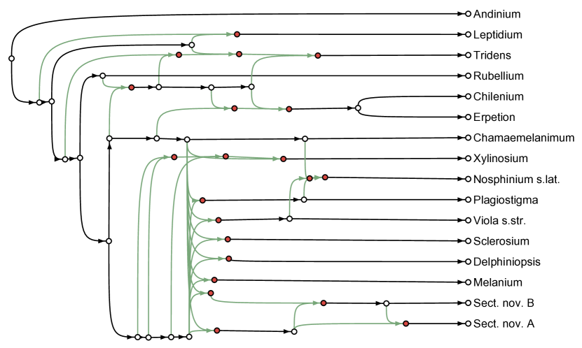
(a) $N$

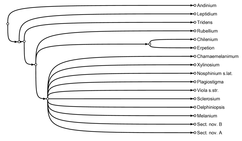
(b) $\varphi_{lsa}(N)$

Figure 3.1: (a) A rooted phylogenetic network $N$ from Jetten and van Iersel, (2018) based on a study from Marcussen et al., (2014) with the reticulate vertices coloured red, and the edges leading to them coloured green. (b) The LSA tree $\varphi_{lsa}(N)$ of $N$.

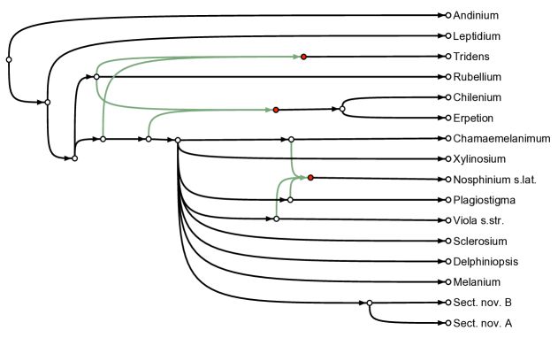
(a) $\varphi_{no}(N)$

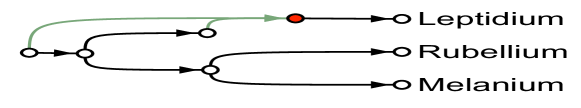
(b) $\varphi_{no}(N|\{\text{Leptidium, Rubellium, Melanium}\})$

(c) $\varphi_{no}(N)|\{\text{Leptidium, Rubellium, Melanium}\}$

Figure 3.2: (a) The normalisation $\varphi_{no}(N)$ of the network $N$ in Fig. 1(a). (b) The normalisation of the restricted network $\varphi_{no}(N|\{\text{Leptidium, Rubellium, Melanium}\}$. (c) The restricted normalisation $\varphi_{no}(N)|\{\text{Leptidium, Rubellium, Melanium}\}$.

4 Concluding comments

In this paper, we have discovered that the LSA tree transformation satisfies all three desirable properties ($P_{1}$–$P_{3}$), whereas several other commonly used transformations fail to satisfy $P_{3}$.

Our results suggest further questions and lines of inquiry. For example, is the LSA tree the only transformation from networks to trees that satisfies $P_{1}$–$P_{3}$ and if not, can one classify the set of such transformations?

Secondly, for the transformation $N\mapsto Ad(t(N))$ described in (3.1), is it possible to compute the $Ad(t(N))$ efficiently (i.e., in polynomial time in $|X|$)? Although computing the Adams consensus of a fixed set of trees can be done in polynomial time, the set $t(N)$ can grow exponentially with the number of reticulation vertices in $N$. More generally, for other consensus tree methods (e.g., strict consensus, majority rule) one can similarly define a transformation from phylogenetic networks to trees based on $t(N)$, so the same question of computational complexity arises for these methods.

Finally, an alternative to transforming arbitrary phylogenetic networks to rooted trees is to consider transformations to other well-behaved network classes that allow for limited reticulation. A particular class of interest is the set of normal networks which have attractive mathematical and computational characteristics (Francis et al., , 2021; Francis, , 2021; Kong et al., , 2022). Thus, it is of interest to consider transformations from arbitrary phylogenetic networks on $X$ to the class of normal networks on $X$ and ask if such transformations can satisfy $P_{1}$, $P_{2}$ and $P_{3}$. For the simple method introduced in Francis et al., (2021), $P_{1}$ and $P_{2}$ hold but $P_{3}$ fails. A counterexample is shown in Fig. 3.2. Whether or not there is a transformation that satisfies all three properties is thus an interesting question. One possible candidate could be the transformation described by Willson, (2022), but we do not consider this further in this paper.

5 Acknowledgements

MS thanks the NZ Marsden Fund for funding support (23-UOC-003).

6 Appendix

We first prove Lemma 2.

Proof.

Let $N\in\mathds{N}(X)$ be any network. Instead of the two subsets $Y$ and $Y^{\prime}$, we consider $S=X\setminus Y$ and $S^{\prime}=Y\setminus Y^{\prime}$. Furthermore, let $N|Y=N^{-S}\in\mathds{N}(X\setminus S)$ denote the network restricted to $Y$. First, Eqn. 6.1 is proven. We then establish Eqn. 2.2 by induction:

$$(N^{-x})^{-S^{\prime}}\cong N^{-(\{x\}\cup S^{\prime})}\text{ with }x\in X,x\notin S^{\prime}.$$ (6.1)

To obtain $N^{-x}$ from $N$, we keep all vertices and edges that are part of any directed path from $lsa_{N}(X\setminus x)$ to any $n\in X\setminus x$. To get $(N^{-x})^{-S^{\prime}}$, we also delete all vertices and edges that lie on any path from $lsa_{N}(X\setminus S^{\prime})$ to any $s\in S^{\prime}$, excluding the ones that are part of a directed path from $lsa_{N}(X\setminus S^{\prime})$ to any $n\in X\setminus S^{\prime}$.

To obtain $N^{-(\{x\}\cup S^{\prime})}$ from $N$, we can proceed the same way as described above because $\{x\}\cap S^{\prime}=\emptyset$, by definition. First, delete $x$. Second, remove $S^{\prime}$. Thus, $(N^{-x})^{-S^{\prime}}\cong N^{-(\{x\}\cup S^{\prime})}$. Eqn. 2.2 can be rephrased as follows:

$$(N^{-S})^{-S^{\prime}}\cong N^{-(S\cup S^{\prime})}.$$ (6.2)

We prove Eqn. 6.2 by induction on $k=|S|$. To start the induction, suppose $k=1$. This case equals Eqn. 6.1 and was proven above. Now, assume that Eqn. 6.2 is true for some $k$. We show that the statement then holds for $k+1$. Suppose that $S=\{s_{1},...,s_{k},s_{k+1}\}$. We have:

$$(N^{-S})^{-S^{\prime}} =(N^{-\{s_{1},...,s_{k},s_{k+1}\}})^{-S^{\prime}}$$ (substitution)

$$=(N^{-(\{s_{1},...,s_{k}\}\cup\{s_{k+1}\})})^{-S^{\prime}}$$ (set operation)

$$\cong((N^{-\{s_{1},...,s_{k}\}})^{-s_{k+1}})^{-S^{\prime}}$$ (induction hypothesis)

$$\cong(N^{-\{s_{1},...,s_{k}\}})^{-(\{s_{k+1}\}\cup S^{\prime})}$$ (Eqn. 6.1)

$$\cong N^{-(\{s_{1},...,s_{k}\}\cup\{s_{k+1}\}\cup S^{\prime})}$$ (induction hypothesis)

$$=N^{-(S\cup S^{\prime})}$$ (substitution)

Eqn. 6.2 is proven, and thereby, Eqn. 2.2. ∎

Secondly, turning to the proof of Proposition 2, Fig. 6.1 provides the counterexample for the transformations $\varphi_{b},\varphi_{c}$ and $\varphi_{tc}$. The counterexample for the transformation $\varphi_{ad}$ is shown in Fig. 6.2.

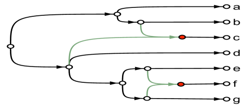
(a) $N$

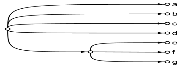
(b) $T=\varphi_{b}(N)=\varphi_{c}(N)=\varphi_{tc}(N)$

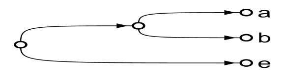
(c) $\varphi_{b,c,tc}(N|\{a,b,e\})$

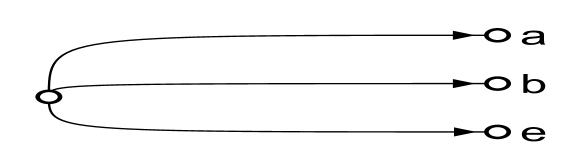
(d) $T|\{a,b,e\}$

Figure 6.1: (a) A rooted phylogenetic network $N\in\mathds{N}(X)$ on leaf set $X=\{a,b,c,d,e,f,g\}$. (b) The blob tree $\varphi_{b}(N)$, the closed tree $\varphi_{c}(N)$ and the result of the tight clusters transformation $\varphi_{tc}(N)$ give rise to the same tree $T$. (c) The restricted network $N|\{a,b,e\}$, which corresponds to its transformation. (d) The restricted tree $T|\{a,b,e\}$.

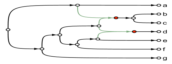
(a) $N$

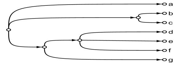
(b) $\varphi_{ad}(N)$

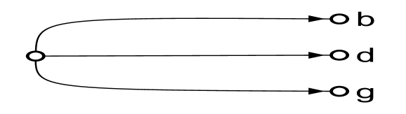
(c) $\varphi_{ad}(N|\{b,d,g\})$

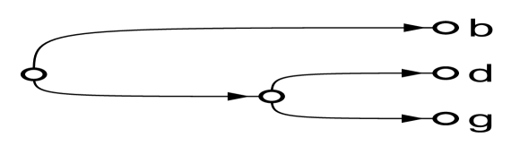
(d) $\varphi_{ad}(N)|\{b,d,g\}$

Figure 6.2: (a) A rooted phylogenetic network $N\in\mathds{N}(X)$ on leaf set $X=\{a,b,c,d,e,f,g\}$. (b) The Adams consensus tree $\varphi_{ad}(N)$ of $N$. (c) The restricted transformed network $\varphi_{ad}(N|\{b,d,g\})$. (d) The restricted Adams consensus tree $\varphi_{ad}(N)|\{b,d,g\}$.

References

- Adams, (1972) E. N. Adams (1972). Consensus techniques and the comparison of taxonomic trees. Systematic Zoology, 21(4):390–397, DOI: 10.2307/2412432.
- Bryant et al., (2017) D. Bryant, A. Francis, and M. Steel (2017). Can we ‘future-proof’ consensus trees? Systematic Biology, 66(4):611--619, DOI: 10.1093/sysbio/syx030.
- Bryant and Steel, (1995) D. Bryant and M. Steel (1995). Extension operations on sets of leaf-labelled trees. Advances in Applied Mathematics, 16(4):425--453, DOI: 10.1006/aama.1995.1020.
- DeSalle and Riley, (2020) R. DeSalle and M. Riley (2020). Should networks supplant tree building? Microorganisms, 8(8):1179, DOI: 10.3390/microorganisms8081179.
- Dress et al., (2010) A. Dress, V. Moulton, M. Steel, and T. Wu (2010). Species, clusters and the ‘tree of life’: a graph-theoretic perspective. Journal of Theoretical Biology, 265(4):535--542, DOI: 10.1016/j.jtbi.2010.05.031.
- Francis, (2021) A. Francis (2021). ‘‘Normal" phylogenetic networks emerge as the leading class. ArXiv: 2107.10414, DOI: 10.48550/arXiv.2107.10414.
- Francis et al., (2021) A. Francis, D. Huson, and M. Steel (2021). Normalising phylogenetic networks. Molecular Phylogenetics and Evolution, 163:107215, DOI: 10.1016/j.ympev.2021.107215.
- Gusfield, (2014) D. Gusfield (2014). ReCombinatorics: The algorithmics of ancestral recombination graphs and explicit phylogenetic networks, pages 201--206. The MIT Press, Cambridge.
- Huber et al., (2019) K. Huber, V. Moulton, and T. Wu (2019). Hierarchies from lowest stable ancestors in nonbinary phylogenetic networks. Journal of Classification, 36(2):200--231, DOI: 10.1007/s00357-018-9279-5.
- Huson et al., (2010) D. Huson, R. Rupp, and C. Scornavacca (2010). Phylogenetic networks: concepts, algorithms and applications. Cambridge University Press, New York.
- Huson and Steel, (2020) D. Huson and M. Steel (2020). PhyloSketch, http://ab.inf.uni-tuebingen.de/software/phylosketch.
- Jetten and van Iersel, (2018) L. Jetten and L. van Iersel (2018). Nonbinary tree-based phylogenetic networks. IEEE/ACM Transactions on Computational Biology and Bioinformatics, 15(1):205--217, DOI: 10.1109/TCBB.2016.2615918.
- Kong et al., (2022) S. Kong, J. Pons, L. Kubatko, and K. Wicke (2022). Classes of explicit phylogenetic networks and their biological and mathematical significance. Journal of Mathematical Biology, 84(6):47, DOI: 10.1007/s00285-022-01746-y.
- Marcussen et al., (2014) T. Marcussen, L. Heier, A. K. Brysting, B. Oxelman, and K. S. Jakobsen (2014). From gene trees to a dated allopolyploid network: Insights from the angiosperm genus Viola (Violaceae). Systematic Biology, 64(1):84--101, DOI: 10.1093/sysbio/syu071.
- Puigbò et al., (2013) P. Puigbò, Y. I. Wolf, and E. V. Koonin (2013). Seeing the tree of life behind the phylogenetic forest. BMC Biology, 11(1):46, DOI: 10.1186/1741-7007-11-46.
- Semple and Toft, (2021) C. Semple and G. Toft (2021). Trinets encode orchard phylogenetic networks. Journal of Mathematical Biology, 83(3):28, DOI: 10.1007/s00285-021-01654-7.
- Steel, (2016) M. Steel (2016). Phylogeny: discrete and random processes in evolution. Society for Industrial and Applied Mathematics, Philadelphia.
- Willson, (2022) S. J. Willson (2022). Merging arcs to produce acyclic phylogenetic networks and normal networks. Bulletin of Mathematical Biology, 84(2):26, DOI: 10.1007/s11538-021-00986-1.
- Wolf et al., (2002) Y. I. Wolf, I. B. Rogozin, N. V. Grishin, and E. V. Koonin (2002). Genome trees and the tree of life. Trends in Genetics, 18(9):472--479, DOI: 10.1016/S0168-9525(02)02744-0.