Stability of Primal-Dual Gradient Flow Dynamics for Multi-Block Convex Optimization Problems

Ibrahim K. Ozaslan, Panagiotis Patrinos, and Mihailo R. Jovanović I. K. Ozaslan and M. R. Jovanović are with the Ming Hsieh Department of Electrical Engineering, University of Southern California, Los Angeles, CA 90089. P. Patrinos is with the Department of Electrical Engineering, Department of Electrical Engineering (ESAT-STADIUS), KU Leuven, 3001 Leuven, Belgium. E-mails: ozaslan@usc.edu, panos.patrinos@esat.kuleuven.be, mihailo@usc.edu.
Abstract

We examine stability properties of primal-dual gradient flow dynamics for composite convex optimization problems with multiple, possibly nonsmooth, terms in the objective function under the generalized consensus constraint. The proposed dynamics are based on the proximal augmented Lagrangian and they provide a viable alternative to ADMM which faces significant challenges from both analysis and implementation viewpoints in large-scale multi-block scenarios. In contrast to customized algorithms with individualized convergence guarantees, we provide a systematic approach for solving a broad class of challenging composite optimization problems. We leverage various structural properties to establish global (exponential) convergence guarantees for the proposed dynamics. Our assumptions are much weaker than those required to prove (exponential) stability of various primal-dual dynamics as well as (linear) convergence of discrete-time methods, e.g., standard two-block and multi-block ADMM and EXTRA algorithms. Finally, we show necessity of some of our structural assumptions for exponential stability and provide computational experiments to demonstrate the convenience of the proposed dynamics for parallel and distributed computing applications.

Index Terms:
Operator splitting, proximal algorithms, gradient flow, primal-dual algorithms, Lyapunov stability, error bound conditions, distributed optimization.

I Introduction

We study the composite constrained optimization problems of the form

$$\begin{array}[]{rcl}\operatorname*{minimize}\limits_{x,\,z}&\!\!\!\!\!\!&{f}(x)\;+\;g(z)\\[2.84544pt] \operatorname*{subject~{}to}&\!\!\!\!\!\!&Ex\,+\,Fz\,-\,q\,=\,0\end{array}$$ (1a)
where $x\in\mathbb{R}^{m}$ and $z\in\mathbb{R}^{n}$ are the optimization variables, $E\in\mathbb{R}^{p\times m}$, $F\in\mathbb{R}^{p\times n}$, and $q\in\mathbb{R}^{p}$ are the problem data, and $f$, $g$ are the separable convex functions given by
$$f(x)\,=\,\sum\limits_{i\,=\,1}^{k}f_{i}(x_{i}),~{}~{}g(z)\,=\,\sum\limits_{j\,=\,1}^{\ell}g_{j}(z_{j}).$$ (1b)

Based on the partition of vectors $x=[x_{1}^{T}~{}\cdots~{}x_{k}^{T}]^{T}$ and $z=[z_{1}^{T}~{}\cdots~{}z_{\ell}^{T}]^{T}$, matrices $E$ and $F$ can also be partitioned conformably as $E=[{E_{1}}{~{}\cdots~{}}{E_{k}}]$ and $F=[{F_{1}}{~{}\cdots~{}}{F_{\ell}}]$. We assume feasibility of problem (1) and denote the set of its solutions by $\mathcal{P}^{\star}$. Furthermore, we let each function $f_{i}$ be convex with a Lipschitz continuous gradient (i.e., smooth) and each $g_{j}$ be closed proper convex (possibly nondifferentiable) function with efficiently computable proximal operators [1]. While we do not assume existence of any smooth terms in the objective function (i.e., we allow $k=0$ in (1b)), if a smooth term exists it should be included in the $x$-block rather than in the $z$-block. This separation between smooth and nonsmooth parts of the objective function plays an important role in identifying weakest set of assumptions that are required to establish our results; it also alleviates cumbersome notation resulting from the introduction of auxiliary variables and demystifies the effect of nondifferentiable components on convergence properties of the underlying algorithms.

Our analyses can be readily carried over to a more general setup in which problem (1) is formulated in a Hilbert space equipped with an inner product and the associated norm. In such cases, constraint matrices $E$ and $F$ are replaced with bounded linear operators. Although we choose to work in the Euclidean space to keep the notation simple and streamline our analysis, we also discuss applications in which the optimization variables are matrices and provide computational experiments for two such applications.

Since the function $g$ is allowed to be nondifferentiable, a wide range of constraints can be included into problem (1). In particular, convex constraints $x_{i}\in\mathcal{X}_{i}$ for some $i\in\{1,\dots,k\}$ can be easily incorporated into (1) by augmenting the objective function with the indicator function of the set $\mathcal{X}_{i}$,

$$\operatorname{I}_{\mathcal{X}_{i}}(x)\;\mathrel{\mathop{:}}=\;\left\{\begin{array}[]{ll}0,&x\,\in\,\mathcal{X}_{i}\\[2.84544pt] \infty&\operatorname*{otherwise}\!.\end{array}\right.$$

For example, linear inequality constraint $G_{i}x_{i}\leq h_{i}$ can be handled by introducing a slack variable $z_{\ell+1}\geq 0$, converting the inequality constraint to the equality constraint $G_{i}x_{i}+z_{\ell+1}=h_{i}$, and by adding the indicator function associated with the positive orthant $g_{\ell+1}(z_{\ell+1})=\operatorname{I}_{\mathbb{R}_{+}}\!(z_{\ell+1})$ to the objective function in (1). Furthermore, even nondifferentiable convex inequality constraints can be included in (1) as long as the projection operator associated with the constraint set is easily computable. In addition to the constrained problems, unconstrained problems of form

$$\operatorname*{minimize}\limits_{x}~{}f(x)\;+\;\sum\limits_{j\,=\,1}^{\ell}g_{j}(T_{j}x)$$ (2)

can also be brought into (1) by setting

$$E\;=\;\left[\begin{array}[]{c}T_{1}\\ T_{2}\\ \vdots\\ T_{\ell}\end{array}\right],~{}F_{1}\;=\;\left[\begin{array}[]{c}{-I}\\ {0}\\ {\vdots}\\ {0}\end{array}\right]~{}\dots~{}~{}F_{\ell}\;=\;\left[\begin{array}[]{c}0\\ \vdots\\ 0\\ -I\end{array}\right],\quad q\;=\;\left[\begin{array}[]{c}0\\ \vdots\\ 0\\ 0\end{array}\right],\quad z_{j}\;=\;T_{j}x,~{}~{}j\;=\;1,\dots,\ell.$$

Optimization problem (1) arises in a host of applications, ranging from signal processing and machine learning to statistics and control theory [2]; see Section II-A. Splitting methods facilitate separate treatment of different blocks in (1) and they provide an effective means for solving this class of problems. If the problem is properly formulated, these methods are also convenient for distributed computations and parallelization. For example, the Alternating Direction of Method of Multipliers (ADMM), which represents a particular instance of more general splitting techniques such as [3, 4, 5, 6, 7], has attracted significant attention because of its straightforward and efficient implementation [2]. The convergence properties of the standard ADMM algorithm are well-understood for two-block problems with $k=\ell=1$ in (1[8]. However, the multi-block case with either $k>1$ or $\ell>1$ is much more subtle and without imposing strong assumptions it is difficult to maintain convergence guarantees [9, 6, 7] and computational convenience [10]. Although variable splitting can be used to bring the multi-block problem into the two-block setup [11], the subproblems can become difficult to solve and the efficiency is compromised because of a significant increase in the number of variables and constraints [12]. Even though various modifications have been proposed for the multi-block ADMM to circumvent strong assumptions that ensure convergence and computational convenience [12, 10, 13, 14], in contrast to standard two-block ADMM the convergence properties of these variations remain unclear in certain scenarios. To the best of our knowledge, sufficient conditions ensuring linear convergence of these variations have not yet been established. Moreover, the empirical evidence suggests that these variations are much slower than the standard multi-block ADMM [15].

The primal-dual (PD) gradient flow dynamics offer a viable alternative to ADMM in terms of implementation: while ADMM requires explicit minimization, only the gradient of the Lagrangian is required to update iterates. Furthermore, in contrast to ADMM, the PD gradient flow dynamics are convenient for parallel and distributed computing even in multi-block problems without requiring any modifications relative to the two-block setup. They are thus appealing for large-scale applications and have attracted significant attention since their introduction as continuous-time dynamical systems in seminal work [16]. Recent effort centered on studying stability and convergence properties of PD gradient flow dynamics under various scenarios. Early results [17, 18] focused on the asymptotic stability of the PD gradient flow dynamics that are based on the Lagrangian associated with differentiable constrained problems. Some of these results have also been extended to general saddle functions [19, 20, 21] and, in a more recent effort, the focus started shifting toward proving the exponential stability [22, 23, 24, 25, 26, 27, 28, 29, 30, 31, 32] and the contraction [33, 34, 35] properties. Also, advancements in Nesterov-type acceleration and design of second-order PD algorithms have been made in [36, 37, 38] and [39], respectively. In particular, [28] introduced a framework to bring the augmented Lagrangian associated with equality constrained convex problems into a smooth form even if the objective function contains nondifferentiable terms. This approach facilitates the use of the PD gradient flow dynamics for nonsmooth problems without resorting to the use of subgradients (which complicate the analysis and substantially slow down convergence).

In this paper, we introduce primal-dual gradient flow dynamics resulting from proximal augmented Lagrangian associated with problem (1). We study asymptotic and exponential stability properties of the underlying dynamics under three different sets of assumptions. Under these assumptions, the proposed dynamics have a continuum of equilibria, which introduces additional challenges for stability analyses relative to the setup with a unique equilibrium point. Our first set of assumptions is much weaker than existing restrictions that are introduced in stability analysis of various primal-dual gradient flow dynamics as well as in convergence analysis of ADMM and EXTRA [40] algorithms. Specifically, without requiring presence of any smooth or strongly convex terms in the objective function and without imposing any additional conditions on the constraint matrices, we show that the primal-dual dynamics are globally asymptotically stable even in the multi-block setup. In our second set of assumptions, we still allow the absence of smooth terms but restrict nonsmooth terms in the objective function to be either a polyhedral function (i.e., the epigraph of such a function can be represented as intersection of finitely many half-spaces) or group lasso penalty function. This allows us to introduce a novel Lyapunov function for establishing local exponential stability of the proposed dynamics and to extend this local result to the semi-global exponential stability; see Remark 1. This result allows us to guarantee exponentially fast global convergence in various challenging problems for which only subexponential rates have been established for gradient-based methods. In our third set of assumptions, we require presence of smooth terms in the objective function and impose additional conditions on the constraint matrices without restricting the class of nonsmooth terms in the objective function. In this setup, we prove the global exponential stability and show that our assumptions are weaker than the conditions used in the literature to prove the exponential stability of primal-dual gradient flow dynamics and linear convergence of ADMM. We then prove that one of the requirements on the constraint matrices indeed represents a necessary condition for global exponential stability of the proposed primal-dual gradient flow dynamics that cannot be relaxed without introducing any additional assumptions on the nonsmooth terms. Finally, in contrast ADMM, we show that the proposed dynamics are amenable to parallel and distributed computing even in multi-block problems without requiring any modifications relative to the two-block setup. Moreover, application of the proposed dynamics to consensus optimization problems leads to distributed implementation similar to those provided in EXTRA and its proximal variant PG-EXTRA [41] algorithms.

Remark 1

Semi-global exponential stability implies global exponential convergence with a rate that depends on the initial distance to the equilibria; see [42, Section 5.10] for definition. While global exponential stability requires the convergence rate and associated constants to be independent of the initial conditions, global exponential convergence follows from a weaker stability notion (i.e., semi-global exponential stability); see (21) and (20), respectively. We also note that notions such as global linear (or geometric) convergence and Q-linear convergence that are used in optimization literature for discrete-time algorithms correspond to the semi-global exponential stability of the underlying nonlinear dynamics.

The rest of the paper is organized as follows. In Section II, we provide motivation and background material and introduce the primal-dual gradient flow dynamics. In Section III, we summarize our main results, discuss related work, and compare our findings with the existing literature. In Section IV, we prove main theorems; in Section V, we utilize computational experiments to demonstrate the merits of our analyses; and in Section VI, we conclude our presentation with remarks.

Notation: We use $\|\cdot\|$ and $\langle\cdot,\cdot\rangle$ to denote the Euclidean norm and standard inner product, \macc@depthΔ\frozen@everymath\macc@group\macc@set@skewchar\macc@nested@a111σ(A)\macc@depthΔ\frozen@everymath\macc@group\macc@set@skewchar\macc@nested@a111𝜎𝐴\macc@depth\char 1\relax\frozen@everymath{\macc@group}\macc@set@skewchar\macc@nested@a 111{\sigma}(A) and $\underline{\sigma}(A)$ to denote the largest and smallest nonzero singular values of a matrix $A$, $\mathcal{N}(A)$ and $\mathcal{R}(A)$ to denote the null and range spaces of $A$, respectively. We define the Euclidean distance between a point $\psi$ and set $\Psi$ as $\operatorname{\mathbf{dist}}(\psi,~{}\Psi)=\min_{\phi\in\Psi}\|\psi-\phi\|^{2}$.

II Motivation and background

We first provide the motivation and background for studying composite optimization problem (1) and then explain how to solve it. In Section II-A, we highlight problem instances that arise in applications. In Section II-B, we provide a brief overview of proximal operators and Moreau envelopes. In Section II-C, we introduce the augmented Lagrangian associated with problem (1) and derive the optimality conditions. In Section II-D, we employ the proximal operators and Moreau envelopes of nonsmooth terms to bring the augmented Lagrangian into a continuously differentiable form that is referred to as the proximal augmented Lagrangian [28]. Finally, in Section II-E, we formulate the primal-dual gradient flow dynamics with a continuous right-hand-side to solve nonsmooth composite optimization problem (1).

II-A Motivating applications

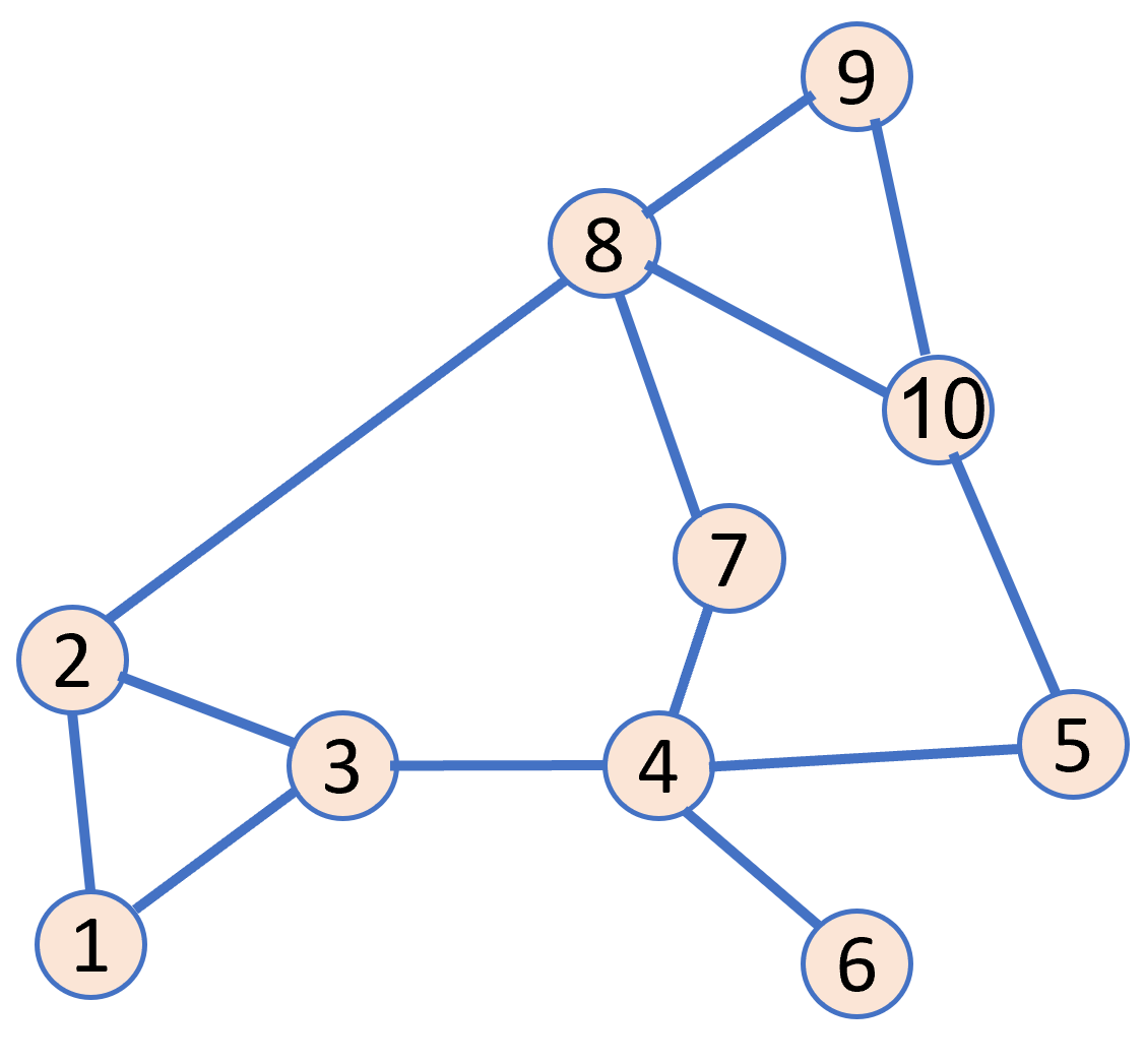
Example 1: Distributed optimization. Various problems in distributed optimization [2] including control and stabilization of power networks [43] and resource allocation in wireless systems [44] can be modeled as a special case of (1). For example, let us consider a regularized consensus problem in which $k$ agents in a connected undirected network aim to cooperatively solve

$$\begin{array}[]{rcl}\operatorname*{minimize}\limits_{\tilde{x}}&\!\!\!\!\!\!&\displaystyle\sum\limits_{i\,=\,1}^{k}\left(f_{i}(\tilde{x})\,+\,g_{i}(C_{i}\tilde{x})\right)\end{array}$$ (3a)
where matrix $C_{i}\in\mathbb{R}^{\widetilde{m}\times\widetilde{n}}$ and convex functions $f_{i}$: $\mathbb{R}^{\widetilde{m}}\to\mathbb{R}$ and $g_{i}$: $\mathbb{R}^{\widetilde{n}}\to\mathbb{R}$, with the former being smooth, are known only by agent $i$. Each vertex in a network represents an agent and each edge represents a communication channel between two agents. The information exchange between two agents occurs only if there exists an edge between the corresponding vertices in the network. If $T^{T}$ denotes the incidence matrix of the connected undirected network, (1b) along with $x\in\mathbb{R}^{k\widetilde{m}}$ and $z\in\mathbb{R}^{k\widetilde{n}}$ can be used to bring this problem along with communication constraints imposed by the network structure into the form (1),
$$\begin{array}[]{rcl}\operatorname*{minimize}\limits_{x,\,z}&\!\!\!\!\!\!&f(x)\,+\,g(z)\\[2.84544pt] \operatorname*{subject~{}to}&\!\!\!\!\!\!&\left[\begin{array}[]{c}T\\ C\end{array}\right]x\,+\,\left[\begin{array}[]{c}0\\ -I\end{array}\right]z\,=\,0\end{array}$$ (3b)

where $Tx=0$ enforces the consensus constraint and $C\mathrel{\mathop{:}}=\operatorname{blkdiag}\,(C_{1},\ldots,C_{k})$. Similar models are also encountered in sharing and optimal exchange problems [2].

Example 2: Principle component pursuit. The following optimization problem arises in the recovery of low rank matrices from noisy incomplete observations [45, 46],

$$\begin{array}[]{rcl}\operatorname*{minimize}\limits_{Z_{1},\,Z_{2},\,Z_{3}}&\!\!\!\!\!\!&\|Z_{1}\|_{\star}\,+\,\gamma_{1}\|Z_{2}\|_{1}\\[2.84544pt] \operatorname*{subject~{}to}&\!\!\!\!\!\!&Z_{1}\,+\,Z_{2}\,+\,Z_{3}\,-\,Q\,=\,0\\[2.84544pt] &\!\!\!\!\!\!&\|P_{\Omega}(Z_{3})\|_{F}\,-\,\gamma_{2}\,\leq\,0\end{array}$$ (4a)
where $Z_{i}$ and $Q$ are matrices of appropriate dimensions, $\gamma_{1}$ and $\gamma_{2}$ are positive parameters, $P_{\Omega}(\cdot)$ is a binary mask that sets entries in the set $\Omega$ to zero, $\|\cdot\|_{\star}$ is the nuclear norm, and $\|\cdot\|_{1}$ is the $\ell_{1}$-norm of a given matrix. This problem can be brought into the form (1) as
$$\begin{array}[]{rcl}\operatorname*{minimize}\limits_{Z_{1},\,Z_{2},\,Z_{3}}&\!\!\!\!\!\!&g_{1}(Z_{1})\,+\,g_{2}(Z_{2})\,+\,g_{3}(Z_{3})\\[2.84544pt] \operatorname*{subject~{}to}&\!\!\!\!\!\!&\left[\begin{array}[]{ccc}I&I&I\end{array}\right]\left[\begin{array}[]{c}Z_{1}\\ Z_{2}\\ Z_{3}\end{array}\right]\,-\,Q\,=\,0\end{array}$$ (4b)

where $g_{1}(Z_{1})=\|Z_{1}\|_{\star}$, $g_{2}(Z_{2})=\gamma_{1}\|Z_{2}\|_{1}$, and $g_{3}(Z_{3})=\operatorname{I}_{\{Z_{3}\,|\,\|P_{\Omega}(Z_{3})\|_{F}\leq\gamma_{2}\}}(Z_{3})$. We note the absence of smooth components in the objective function. Similar models also arise in the estimation of sparse inverse covariance matrices [47] and in the alignment of linearly correlated images under corruption [48].

Example 3: Covariance completion. The following problem is introduced for identification of low-complexity disturbance models that account for partially available second-order statistics of dynamical systems [49, 50, 51],

$$\begin{array}[]{rcl}\operatorname*{minimize}\limits_{X,\,Z}&\!\!\!\!\!\!&-\log\det(X)\,+\,\gamma\|Z\|_{\star}\\[2.84544pt] \operatorname*{subject~{}to}&\!\!\!\!\!\!&AX\,+\,AX^{T}\,+\,Z\,=\,0\\[2.84544pt] &\!\!\!\!\!\!&(BXB^{T})\circ C\,-\,Q\,=\,0\end{array}$$ (5a)
where $X$, $Z$, $A$, $B$, $C$, and $Q$ are matrices of appropriate dimensions, $\gamma$ is a positive parameter, and $\circ$ denotes the Hadamard product. This problem can be recast into the form (1) as
$$\begin{array}[]{rcl}\operatorname*{minimize}\limits_{X,\,Z}&\!\!\!\!\!\!&f(X)\,+\,g(Z)\\[2.84544pt] \operatorname*{subject~{}to}&\!\!\!\!\!\!&\left[\begin{array}[]{c}\mathcal{E}_{1}\\ \mathcal{E}_{2}\end{array}\right]X\,+\,\left[\begin{array}[]{c}I\\ 0\end{array}\right]Z\,=\,\left[\begin{array}[]{c}0\\ Q\end{array}\right]\end{array}$$ (5b)

where $f(X)=-\log\det(X+\delta I)$, $g(Z)=\|Z\|_{\star}$, with the linear operators defined as $\mathcal{E}_{1}(X)=AX+XA^{T}$ and $\mathcal{E}_{2}(X)=(BXB^{T})\circ C$. We use additional regularization parameter $\delta$ to ensure that $f$ is a smooth convex function. The optimization variables in (5) are matrices and generalized consensus constraint in (1) is expressed using linear operators $\mathcal{E}_{1}$ and $\mathcal{E}_{2}$. Even though the conversion to a vectorized form is straightforward, working with the matricial formulation is advantageous from both conceptual and implementation viewpoints.

Example 4: Exact convex formulation of neural networks. The following problem emerges in the convex formulation of connected two layer neural networks with ReLU activation [52],

$$\begin{array}[]{rcl}\operatorname*{minimize}\limits_{u,\,\tilde{u}}&\!\!\!\!\!\!&\displaystyle h\left(\sum_{i\,=\,1}^{r}T_{i}(u_{i}\,-\,\tilde{u}_{i}),\,q\right)\,+\,\gamma\sum_{i\,=\,1}^{r}(\|u_{i}\|\,+\,\|\tilde{u}_{i}\|)\\[2.84544pt] \operatorname*{subject~{}to}&\!\!\!\!\!\!&G_{i}u_{i}\,\geq\,0\qquad i\,=\,1,\ldots,r\\[2.84544pt] &\!\!\!\!\!\!&G_{i}\tilde{u}_{i}\,\geq\,0\qquad i\,=\,1,\ldots,r\end{array}$$ (6a)
where $u=[u_{1}^{T}{~{}\cdots~{}}u_{r}^{T}]^{T}$ and $\tilde{u}=[\tilde{u}_{1}^{T}{~{}\cdots~{}}\tilde{u}_{r}^{T}]^{T}$, $h(\cdot,\cdot)$ is a smooth loss function, $q$ is the vector of labels, $T_{i}$’s and $G_{i}$’s are given matrices of appropriate dimensions, and $\gamma$ is a positive parameter. Using the following definitions [53],
$$x_{2}\,\mathrel{\mathop{:}}=\,[u^{T}{~{}}\tilde{u}^{T}]^{T},\quad T\,\mathrel{\mathop{:}}=\,[T_{1}{~{}\cdots~{}}T_{r}\;-T_{1}{~{}\cdots~{}}-T_{r}],\quad G\,\mathrel{\mathop{:}}=\,\operatorname{blkdiag}\,(G_{1},\ldots,G_{r},G_{1},\ldots,G_{r})$$
we transform this problem into the form (1),
$$\begin{array}[]{rcl}\operatorname*{minimize}\limits_{x,\,z}&\!\!\!\!\!\!&f_{1}(x_{1})\,+\,\gamma\|z_{1}\|_{1,2}\,+\,\operatorname{I}_{\mathbb{R}_{+}}(z_{2})\\[2.84544pt] \operatorname*{subject~{}to}&\!\!\!\!\!\!&\left[\begin{array}[]{cc}0&I\\ 0&G\\ -I&T\end{array}\right]\left[\begin{array}[]{c}x_{1}\\ x_{2}\end{array}\right]\,+\,\left[\begin{array}[]{cc}-I&0\\ 0&-I\\ 0&0\end{array}\right]\left[\begin{array}[]{c}z_{1}\\ z_{2}\end{array}\right]\,=\,0\end{array}$$ (6b)

where $x_{1}$ is the auxiliary variable, $f_{1}(x_{1})=h(x_{1},q)$, and $\|\cdot\|_{1,2}$ is the group lasso penalization. Similar formulations can also be found in the context of empirical risk minimization such as sparse-group lasso where both $\ell_{1,2}$- and $\ell_{1}$-norm penalization appear in the objective function [54].

II-B The proximal operator and the Moreau envelope

The proximal operator associated with a proper closed convex function $g$ is the mapping defined as [1],

$$\operatorname{\mathbf{prox}}_{\mu g}(\nu)\,=\,(I\,+\,\mu\partial g)^{-1}(\nu)$$ (7)

where $\mu$ is a positive parameter and $\partial g$ is the subdifferential of $g$ [55, Chapter 16]. Alternatively, $\operatorname{\mathbf{prox}}_{\mu g}$ can be obtained as the minimizer of the following optimization problem,

$$\operatorname{\mathbf{prox}}_{\mu g}(\nu)\,=\,\operatorname*{argmin}\limits_{w}~{}g(w)\,+\,\tfrac{1}{2\mu}\|w\,-\,\nu\|^{2}.$$

The value function of this optimization problem determines the associated Moreau envelope of $g$

$$M_{\mu g}(\nu)\,\mathrel{\mathop{:}}=\,g(\operatorname{\mathbf{prox}}_{\mu g}(\nu))\,+\,\tfrac{1}{2\mu}\|\operatorname{\mathbf{prox}}_{\mu g}(\nu)\,-\,\nu\|^{2}$$ (8)

which is a continuously-differentiable function, even for nondifferentiable $g$, with $1/\mu$-Lipschitz continuous gradient [55, Proposition 12.30],

$$\nabla M_{\mu g}(\nu)\,=\,\tfrac{1}{\mu}(\nu\,-\,\operatorname{\mathbf{prox}}_{\mu g}(\nu)).$$

By partitioning vector $\nu$ as $\nu\mathrel{\mathop{:}}=[{\nu_{1}^{T}}{~{}\cdots~{}}{\nu_{\ell}^{T}}]^{T}$, separable structure in (1b) can be used to obtain,

$$\operatorname{\mathbf{prox}}_{\mu g}(\nu)\,=\,\left[\begin{array}[]{c}\operatorname{\mathbf{prox}}_{\mu g_{1}}(\nu_{1})\\ \vdots\\ \operatorname{\mathbf{prox}}_{\mu g_{\ell}}(\nu_{\ell})\end{array}\right],~{}~{}M_{\mu g}(\nu)\,=\,\sum\limits_{i\,=\,1}^{\ell}M_{\mu g_{i}}(\nu_{i}).$$ (9)

II-C Lagrange saddle function

Optimization problem (1) can be lifted to a higher dimensional space by introducing auxiliary variables $w_{i}$ for each nonsmooth block associated with $z_{i}$,

$$\begin{array}[]{rcl}\operatorname*{minimize}\limits_{x,\,z,\,w}&\!\!\!\!\!\!&f(x)\,+\,g(w)\\[2.84544pt] \operatorname*{subject~{}to}&\!\!\!\!\!\!&Ex\,+\,Fz\,-\,q\,=\,0\\[2.84544pt] &\!\!\!\!\!\!&z\,-\,w\,=\,0\end{array}$$ (10)

where $w=[{w_{1}^{T}}{~{}\cdots~{}}{w_{\ell}^{T}}]^{T}\in\mathbb{R}^{n}$. The auxiliary variables in (10) isolate each nonsmooth block in the objective function and facilitate the derivation of a continuously-differentiable saddle function in Section II-D. We denote the set of all solutions to (10) by $\mathcal{P}^{\star}_{w}$; clearly, $\mathcal{P}^{\star}_{w}=\{(x,z,z)|(x,z)\in\mathcal{P}^{\star}\}$ and, throughout the manuscript, we use the subscript $(\,\cdot\,)_{\omega}$ to highlight that the solution set is associated with the lifted problem.

Associating the dual variable $y_{i}$ with $z_{i}-w_{i}=0$ for each $i=1,\ldots,\ell$, and the dual variable $\lambda\in\mathbb{R}^{p}$ with the linear equality constraint $Ex+Fz-q=0$ yields the following Lagrange saddle function for problem (10),

$$\mathcal{L}(x,z,w;y,\lambda)\,=\,f(x)\,+\,g(w)\,+\,\lambda^{T}(Ex\,+\,Fz\,-\,q)\,+\,y^{T}(z\,-\,w)$$ (11)

where $y=[{y_{1}^{T}}{~{}\cdots~{}}{y_{\ell}^{T}}]^{T}\in\mathbb{R}^{n}$. Throughout the paper, we assume that there exists $(x,z)\in\mathbb{R}^{m}\times\mathbf{ri}\operatorname{\mathbf{dom}}g$ such that $Ex+Fz=q$, where $\mathbf{ri}\operatorname{\mathbf{dom}}g$ denotes the relative interior of domain of $g$ [55, Section 6.2]. This assumptions ensures that the strong duality holds [55, Theorem 15.23 and Proposition 15.24(x)]. Consequently, the necessary and sufficient conditions for $(x^{\star},z^{\star},w^{\star},y^{\star},\lambda^{\star})$ to be an optimal primal-dual pair of problem (10) are given by the Karush-Kuhn-Tucker (KKT) conditions,

$\displaystyle\nabla f(x^{\star})$ $\displaystyle\!\!\!=\!\!\!$ $\displaystyle-E^{T}\lambda^{\star}$ (12a)
$\displaystyle y^{\star}$ $\displaystyle\!\!\!=\!\!\!$ $\displaystyle-F^{T}\lambda^{\star}$ (12b)
$\displaystyle\partial g(w^{\star})$ $\displaystyle\!\!\!\ni\!\!\!$ $\displaystyle y^{\star}$ (12c)
$\displaystyle z^{\star}$ $\displaystyle\!\!\!=\!\!\!$ $\displaystyle w^{\star}$ (12d)
$\displaystyle q$ $\displaystyle\!\!\!=\!\!\!$ $\displaystyle Ex^{\star}\,+\,Fz^{\star}.$ (12e)

Let $\Psi^{\star}_{w}$ denote the set of all points satisfying optimality conditions (12). Since the KKT system (12) is challenging to solve because of nonlinear inclusions (12a) and (12c), we utilize the fact that every solution $(x^{\star},z^{\star},w^{\star},y^{\star},\lambda^{\star})\in\Psi^{\star}_{w}$ is a saddle point of the Lagrangian that satisfies,

$$\mathcal{L}_{\mu}(x^{\star},z^{\star},w^{\star};y,\lambda)\,\leq\,\mathcal{L}_{\mu}(x^{\star},z^{\star},w^{\star};y^{\star},\lambda^{\star})\,\leq\,\mathcal{L}_{\mu}(x,z,w;y^{\star},\lambda^{\star}),\quad\forall x,z,w,y,\lambda.$$ (13)

Based on this characterization, a solution to (10) can be computed by simultaneous minimization and maximization of the Lagrangian over primal variables $(x,z,w)$ and dual variables $(y,\lambda)$, respectively. In what follows, we describe how the underlying problem structure can be exploited to formulate a continuously-differentiable Lagrange saddle function and develop primal-dual algorithms with superior performance relative to the first-order methods that utilize subgradients (which suffer from slow convergence rate even for strongly convex problems; e.g., see [56, Section 3.4]).

II-D Proximal augmented Lagrangian

Computation of saddle points that satisfy (13) is, in general, a challenging task because of the presence of nondifferentiable terms. We can alleviate these difficulties by exploiting the structure of the associated proximal operator that yields the manifold on which the augmented Lagrangian is minimized with respect to the auxiliary variable $w$. The augmented Lagrangian, which has the same saddle points as (11), is obtained by adding a quadratic penalty to (11) for each equality constraint in (10),

$$\mathcal{L}_{\mu}(x,z,w;y,\lambda)\,=\,f(x)\,+\,g(w)\,+\,\lambda^{T}(Ex\,+\,Fz\,-\,q)\,+\,y^{T}(z\,-\,w)\,+\,\tfrac{1}{2\mu}\|Ex\,+\,Fz\,-\,q\|^{2}\,+\,\tfrac{1}{2\mu}\|z\,-\,w\|^{2}$$

where $\mu$ is a positive penalty parameter. Completion of squares yields

$$\mathcal{L}_{\mu}(x,z,w;y,\lambda)\,=\,f(x)\,+\,g(w)\,+\,\tfrac{1}{2\mu}\|w\,-\,(z\,+\,\mu y)\|^{2}\,+\,\tfrac{1}{2\mu}\|Ex\,+\,Fz\,-\,q\,+\,\mu\lambda\|^{2}\,-\,\tfrac{\mu}{2}\|y\|^{2}\,-\,\tfrac{\mu}{2}\|\lambda\|^{2}$$ (14)

and the explicit minimizer of $\mathcal{L}_{\mu}$ with respect to $w$ is determined by the proximal operator of the function $g$,

\macc@depthΔ\frozen@everymath\macc@group\macc@set@skewchar\macc@nested@a111w(z;y):=argminwμ(x,z,w;y,λ)=𝐩𝐫𝐨𝐱μg(z+μy).\macc@depth\char 1\relax\frozen@everymath{\macc@group}\macc@set@skewchar\macc@nested@a 111{w}(z;y)\,\mathrel{\mathop{:}}=\,\operatorname*{argmin}\limits_{w}~{}\mathcal{L}_{\mu}(x,z,w;y,\lambda)\,=\,\operatorname{\mathbf{prox}}_{\mu g}(z\,+\,\mu y). (15)

From Section II-B, we recall that $M_{\mu g}(\nu)\mathrel{\mathop{:}}=g(\operatorname{\mathbf{prox}}_{\mu g}(\nu))+\tfrac{1}{2\mu}\|\operatorname{\mathbf{prox}}_{\mu g}(\nu)-\nu\|^{2}$ which allows us to perform the explicit minimization of the augmented Lagrangian over $w$ and obtain the saddle function that is referred to as the proximal augmented Lagrangian [28],

μ(x,z;y,λ):=minimizewμ(x,z,w;y,λ)=μ(x,z,\macc@depthΔ\frozen@everymath\macc@group\macc@set@skewchar\macc@nested@a111w(z;y);y,λ)=f(x)+Mμg(z+μy)+12μEx+Fzq+μλ2μ2y2μ2λ2.subscript𝜇𝑥𝑧𝑦𝜆:absentsubscriptminimize𝑤subscript𝜇𝑥𝑧𝑤𝑦𝜆subscript𝜇𝑥𝑧\macc@depthΔ\frozen@everymath\macc@group\macc@set@skewchar\macc@nested@a111𝑤𝑧𝑦𝑦𝜆missing-subexpression𝑓𝑥subscript𝑀𝜇𝑔𝑧𝜇𝑦12𝜇superscriptnorm𝐸𝑥𝐹𝑧𝑞𝜇𝜆2𝜇2superscriptnorm𝑦2𝜇2superscriptnorm𝜆2\begin{array}[]{rcl}\mathcal{L}_{\mu}(x,z;y,\lambda)&\!\!\!\mathrel{\mathop{:}}=\!\!\!&\operatorname*{minimize}\limits_{w}~{}\mathcal{L}_{\mu}(x,z,w;y,\lambda)\,=\,\mathcal{L}_{\mu}(x,z,\macc@depth\char 1\relax\frozen@everymath{\macc@group}\macc@set@skewchar\macc@nested@a 111{w}(z;y);y,\lambda)\\[2.84544pt] &\!\!\!=\!\!\!&\displaystyle f(x)\,+\,M_{\mu g}(z\,+\,\mu y)\,+\,\tfrac{1}{2\mu}\|Ex\,+\,Fz\,-\,q\,+\,\mu\lambda\|^{2}\,-\,\tfrac{\mu}{2}\|y\|^{2}\,-\,\tfrac{\mu}{2}\|\lambda\|^{2}.\end{array} (16)

In contrast to the augmented Lagrangian which is a nonsmooth function of $w$, the proximal augmented Lagrangian has Lipschitz continuous gradients with respect to both primal ($x,z$) and dual ($y,\lambda$) variables. Moreover, as detailed in the next section, the set of saddle points of the proximal augmented Lagrangian, which is denoted by $\Psi^{\star}$, together with (15) yields the set of points $\Psi^{\star}_{w}$ that satisfy KKT conditions (12).

II-E Primal-dual gradient flow dynamics

Since the proximal augmented Lagrangian is a continuously differentiable saddle function, first-order algorithms can be used to compute its saddle points. In particular, we utilize primal-descent dual-ascent gradient flow dynamics,

$\displaystyle\dot{x}$ $\displaystyle\!\!\!=\!\!\!$ $\displaystyle-\nabla_{x}\mathcal{L}_{\mu}(x,z;y,\lambda)\,=\,-\,\nabla f(x)\,-\,E^{T}(\lambda\,+\,\tfrac{1}{\mu}(Ex\,+\,Fz\,-\,q))$ (17a)
$\displaystyle\dot{z}$ $\displaystyle\!\!\!=\!\!\!$ $\displaystyle-\nabla_{z}\mathcal{L}_{\mu}(x,z;y,\lambda)\,=\,-\,\nabla_{z}M_{\mu g}(z\,+\,\mu y)\,-\,F^{T}(\lambda\,+\,\tfrac{1}{\mu}(Ex\,+\,Fz\,-\,q))$ (17b)
$\displaystyle\dot{y}$ $\displaystyle\!\!\!=\!\!\!$ $\displaystyle\alpha\nabla_{y}\mathcal{L}_{\mu}(x,z;y,\lambda)\,=\,\alpha\left(\nabla_{y}M_{\mu g}(z\,+\,\mu y)\,-\,\mu y\right)$ (17c)
$\displaystyle\dot{\lambda}$ $\displaystyle\!\!\!=\!\!\!$ $\displaystyle\alpha\nabla_{\lambda}\mathcal{L}_{\mu}(x,z;y,\lambda)\,=\,\alpha\left(Ex\,+\,Fz\,-\,q\right)$ (17d)

where $x$: $[t_{0},\infty)\to\mathbb{R}^{m}$, $z$: $[t_{0},\infty)\to\mathbb{R}^{n}$, $y$: $[t_{0},\infty)\to\mathbb{R}^{n}$, $\lambda$: $[t_{0},\infty)\to\mathbb{R}^{p}$, $t_{0}$ is the initial time, and $\alpha$ is the positive parameter that determines the time constant of the dual dynamics. We denote the state vector in (17) by $\psi=(x,z,y,\lambda)$.

By construction, the equilibrium points of primal-dual gradient flow dynamics (17) are the saddle points of the proximal augmented Lagrangian which in conjunction with (15) satisfy KKT conditions (12). To show this, we set the right-hand-side of (17) to zero. Equation (17d) gives condition (12e). Equation (17c) yields $z=\operatorname{\mathbf{prox}}_{\mu g}(z+\mu y)$ which together with (15) implies (12d). Furthermore, by the definition of proximal operator (7), $z=\operatorname{\mathbf{prox}}_{\mu g}(z+\mu y)$ is equivalent to $y\in\partial g(z)$ which together with (12d) results in (12c). Equation (17b) together with (17c) and (12e) yields (12b). Finally, equation (17a) combined with (17d) provides (12a).

Remark 2

Separable structure in (1b) combined with (9) allows us to recast (17) in terms of individual blocks,

$$\begin{array}[]{rclr}\dot{\lambda}&\!\!\!=\!\!\!&\displaystyle\alpha\big{(}\sum_{i\,=\,1}^{k}E_{i}x_{i}\,+\,\sum_{j\,=\,1}^{\ell}F_{j}z_{j}\,-\,q\big{)}\\[2.84544pt] \dot{y}_{j}&\!\!\!=\!\!\!&\alpha\big{(}(z_{j}\,-\,\operatorname{\mathbf{prox}}_{\mu g_{j}}(z_{j}\,+\,\mu y_{j})\big{)}&\qquad j\,=\,1,\dots,\ell\\[2.84544pt] \dot{z}_{j}&\!\!\!=\!\!\!&-\,(y_{j}\,+\,\tfrac{1}{\alpha\mu}\dot{y}_{j})\,-\,F_{j}^{T}(\lambda\,+\,\tfrac{1}{\alpha\mu}\dot{\lambda})&\qquad j\,=\,1,\dots,\ell\\[2.84544pt] \dot{x}_{i}&\!\!\!=\!\!\!&-\,\nabla f(x_{i})\,-\,E_{i}^{T}(\lambda\,+\,\tfrac{1}{\alpha\mu}\dot{\lambda})&\qquad i\,=\,1,\dots,k\end{array}$$ (18)

where the derivatives of $\lambda$ and $y_{j}$ on the right-hand-side of (18) are used for notational convenience. Here, once $\lambda$-block is computed, each $x_{i}$-block can be implemented in parallel to other $x$-blocks as well as to $y$- and $z$-blocks. Similarly, each $y_{j}$- and $z_{j}$-block can be computed in parallel to other $y$- and $z$-blocks. In Section III-B3, we also illustrate the convenience of (17) for distributed optimization.

III Main results and discussion

In this section, we summarize our main results and compare our contributions to the existing literature. Our first theorem in Section III-A establishes Global Asymptotic Stability (GAS) of primal-dual gradient flow dynamics (17) under Assumption 1, which only requires feasibility and convexity of problem (1). In Theorem 2, we restrict the class of functions in (1) to establish Local Exponential Stability (LES) result. In particular, we assume that (i) the smooth blocks in (1) are not only convex but also satisfy the Polyak-Lojasiewicz (PL) condition (Assumption 2); (ii) the nonsmooth blocks are either polyhedral, i.e., their epigraph can be represented as intersection of finitely many halfspaces or they are given by a group lasso penalty function (Assumption 3). Remarkably, Theorem 2 proves exponential stability for a continuum of equilibria without introducing any assumption on the constraint matrices $E$ and $F$. Combining this result with GAS, in Corollary 1, we establish the Semi-Global Exponential Stability (Semi-GES) of the primal-dual gradient flow dynamics. It should be noted that while Semi-GES guarantees exponentially fast global convergence to the equilibrium points, the rate of convergence depends on the initial distance to the equilibrium points; see [42, Section 5.10] or (20) for the definition.

In Theorem 3, we prove the Global Exponential Stability (GES) of primal-dual gradient flow dynamics (17). While strong convexity of the objective function along with the invertibility of matrices $EE^{T}$ and $F$ in (1) is typically required to establish GES of primal-dual dynamics associated with the class of problems (1[28], we identify different structural requirements on the constraint matrices $E$ and $F$ that allow us to relax these assumptions. Our requirements, summarized in Assumptions 4 and 5, ensure strong convexity of the proximal augmented Lagrangian with respect to the primal variables and allow for the rows of the matrix $E$ to be linearly dependent as long as the range space of $F$ is contained in the range space of $E$. Furthermore, in contrast to Theorem 2, in Theorem 3 we prove exponential stability for the equilibrium points that form an affine set without introducing any additional restrictions on the nonsmooth blocks. Finally, in Theorem 4, we show that Assumption 5 is indeed necessary for GES of the primal-dual gradient flow dynamics applied to problem (1); this assumption cannot be relaxed without introducing additional restrictions on the nonsmooth blocks.

In Section III-B, we compare and contrast our results with the existing literature on primal-dual gradient flow dynamics and ADMM. The comparison with ADMM is fair because a proper discretization of exponentially stable primal-dual algorithm (17) can be used to obtain a linearly convergent discrete-time algorithm; see [22, Lemma 5] and [27] for details. Furthermore, since our primary goal is to identify the weakest structural properties that enable exponentially fast convergence of primal-dual gradient flow dynamics, the existing conditions that guarantee linear convergence of ADMM are particularly informative to understand merits of our results.

Finally, in Section III-C, we show that in contrast to ADMM, the primal-dual gradient flow dynamics are convenient for parallel and distributed computing even in multi-block problems without requiring any modifications relative to the two-block setup. For this purpose we show that the application of (17) to consensus optimization problem (3) leads to distributed implementation similar to those provided in EXTRA and its proximal variant PG-EXTRA [41] algorithms. However, in contrast to EXTRA and PG-EXTRA, the global convergence results summarized in Section III are all readily applicable to the distributed dynamics. In particular, Corollary 1 guarantees exponentially fast global convergence of the distributed dynamics even in the presence of nonsmooth blocks in the objective function.

III-A Summary of main results

Assumption 1 (constraint qualification)

There exists $(x,z)\in\mathbb{R}^{m}\times\mathbf{ri}\operatorname{\mathbf{dom}}g$ such that $Ex+Fz=q$; the function $f$ is convex with an $L_{f}$-Lipschitz continuous gradient $\nabla f$; and the function $g$ is proper, closed, and convex.

Theorem 1 (GAS)

Let Assumption 1 hold. The set of equilibrium points $\Psi^{\star}$ of primal-dual gradient flow dynamics (17), characterized by KKT conditions (12), is globally asymptotically stable and the solution to (17) converges to a point in this set.

Proof:

See Section IV-A. ∎

Assumption 2 (Relaxation of strong convexity)

Each smooth component in (1b) is given by $f_{i}(x_{i})=h_{i}(A_{i}x_{i})$ for all $i=1,\dots,k$ where $x_{i}\in\mathbb{R}^{m_{i}}$, $h_{i}$: \macc@depthΔ\frozen@everymath\macc@group\macc@set@skewchar\macc@nested@a111misuperscript\macc@depthΔ\frozen@everymath\macc@group\macc@set@skewchar\macc@nested@a111subscript𝑚𝑖\mathbb{R}^{\macc@depth\char 1\relax\frozen@everymath{\macc@group}\macc@set@skewchar\macc@nested@a 111{m}_{i}}\to\mathbb{R} is a strongly convex function with a Lipschitz continuous gradient, and Ai\macc@depthΔ\frozen@everymath\macc@group\macc@set@skewchar\macc@nested@a111mi×misubscript𝐴𝑖superscript\macc@depthΔ\frozen@everymath\macc@group\macc@set@skewchar\macc@nested@a111subscript𝑚𝑖subscript𝑚𝑖A_{i}\in\mathbb{R}^{\macc@depth\char 1\relax\frozen@everymath{\macc@group}\macc@set@skewchar\macc@nested@a 111{m}_{i}\times m_{i}} is a (possibly zero) matrix.

Remark 3

Since $A_{i}$’s in Assumption 2 are not assumed to be full-column rank, the smooth block $f$ in (1) is not necessarily a strongly convex function; it is even allowed to have $f=0$.

Assumption 3 (Restriction of nonsmooth functions)

Each nonsmooth component in (1b) is either (i) a polyhedral function or (ii) a group lasso penalization, i.e., $g_{j}(z_{j})=\eta\|z_{j}\|_{1}+\sum_{\mathcal{J}}\omega_{\mathcal{J}}\|z_{\mathcal{J}}\|$, where $z_{j}\in\mathbb{R}^{n_{j}}$, $\omega_{\mathcal{J}}>0$, and $\mathcal{J}$ is an index partition of $\{1,\ldots,n_{j}\}$.

Remark 4

Functions that are frequently used in optimization, control, and machine learning that satisfy Assumption 3 include, but are not limited to, hinge loss, piecewise affine functions (e.g., $\ell_{1}$ and $\ell_{\infty}$ norms), indicator functions of polyhedral sets (i.e., sets associated with linear equality and inequality constraints), and $\ell_{1,2}$-norm regularization. Under additional complementary-type constraint qualifications on $\Psi^{\star}$, even nuclear norm $\|\cdot\|_{\star}$ can be included in this list [57, Proposition 12].

Theorem 2 (LES)

Let Assumptions 12, and 3 hold. There exists a time \macc@depthΔ\frozen@everymath\macc@group\macc@set@skewchar\macc@nested@a111t(t0,)\macc@depthΔ\frozen@everymath\macc@group\macc@set@skewchar\macc@nested@a111𝑡subscript𝑡0\macc@depth\char 1\relax\frozen@everymath{\macc@group}\macc@set@skewchar\macc@nested@a 111{t}\in(t_{0},\infty) such that for α(0,\macc@depthΔ\frozen@everymath\macc@group\macc@set@skewchar\macc@nested@a111α1)𝛼0\macc@depthΔ\frozen@everymath\macc@group\macc@set@skewchar\macc@nested@a111subscript𝛼1\alpha\in(0,\macc@depth\char 1\relax\frozen@everymath{\macc@group}\macc@set@skewchar\macc@nested@a 111{\alpha}_{1}), any solution $\psi(t)$ to primal-dual gradient flow dynamics (17) satisfy

𝐝𝐢𝐬𝐭(ψ(t),Ψ)M1𝐝𝐢𝐬𝐭(ψ(\macc@depthΔ\frozen@everymath\macc@group\macc@set@skewchar\macc@nested@a111t),Ψ)eρ1(t\macc@depthΔ\frozen@everymath\macc@group\macc@set@skewchar\macc@nested@a111t),t\macc@depthΔ\frozen@everymath\macc@group\macc@set@skewchar\macc@nested@a111t.formulae-sequence𝐝𝐢𝐬𝐭𝜓𝑡superscriptΨsubscript𝑀1𝐝𝐢𝐬𝐭𝜓\macc@depthΔ\frozen@everymath\macc@group\macc@set@skewchar\macc@nested@a111𝑡superscriptΨsuperscriptesubscript𝜌1𝑡\macc@depthΔ\frozen@everymath\macc@group\macc@set@skewchar\macc@nested@a111𝑡for-all𝑡\macc@depthΔ\frozen@everymath\macc@group\macc@set@skewchar\macc@nested@a111𝑡\operatorname{\mathbf{dist}}(\psi(t),\Psi^{\star})\,\leq\,M_{1}\operatorname{\mathbf{dist}}(\psi(\macc@depth\char 1\relax\frozen@everymath{\macc@group}\macc@set@skewchar\macc@nested@a 111{t}),\Psi^{\star})\mathrm{e}^{-\rho_{1}(t\,-\,\macc@depth\char 1\relax\frozen@everymath{\macc@group}\macc@set@skewchar\macc@nested@a 111{t})},\quad\forall t\,\geq\,\macc@depth\char 1\relax\frozen@everymath{\macc@group}\macc@set@skewchar\macc@nested@a 111{t}. (19)

Constants \macc@depthΔ\frozen@everymath\macc@group\macc@set@skewchar\macc@nested@a111t\macc@depthΔ\frozen@everymath\macc@group\macc@set@skewchar\macc@nested@a111𝑡\macc@depth\char 1\relax\frozen@everymath{\macc@group}\macc@set@skewchar\macc@nested@a 111{t}, \macc@depthΔ\frozen@everymath\macc@group\macc@set@skewchar\macc@nested@a111α1\macc@depthΔ\frozen@everymath\macc@group\macc@set@skewchar\macc@nested@a111subscript𝛼1\macc@depth\char 1\relax\frozen@everymath{\macc@group}\macc@set@skewchar\macc@nested@a 111{\alpha}_{1}, $M_{1}$, and $\rho_{1}$ are characterized in the proof; see (40). Among these constants, only \macc@depthΔ\frozen@everymath\macc@group\macc@set@skewchar\macc@nested@a111t\macc@depthΔ\frozen@everymath\macc@group\macc@set@skewchar\macc@nested@a111𝑡\macc@depth\char 1\relax\frozen@everymath{\macc@group}\macc@set@skewchar\macc@nested@a 111{t} depends on the initial distance $\operatorname{\mathbf{dist}}(\psi(t_{0}),\Psi^{\star})$.

Proof:

See Section IV-B. ∎

Theorem 2 in conjunction with Theorem 1 implies existence of an exponentially decaying global upper bound on the distance to the equilibrium points. Since this upper bound depends on the initial distance to the equilibirum points, it implies semi-global exponential stability.

Corollary 1 (Semi-GES)

Let Assumptions 12, and 3 hold. For α(0,\macc@depthΔ\frozen@everymath\macc@group\macc@set@skewchar\macc@nested@a111α1)𝛼0\macc@depthΔ\frozen@everymath\macc@group\macc@set@skewchar\macc@nested@a111subscript𝛼1\alpha\in(0,\macc@depth\char 1\relax\frozen@everymath{\macc@group}\macc@set@skewchar\macc@nested@a 111{\alpha}_{1}) where \macc@depthΔ\frozen@everymath\macc@group\macc@set@skewchar\macc@nested@a111α1>0\macc@depthΔ\frozen@everymath\macc@group\macc@set@skewchar\macc@nested@a111subscript𝛼10\macc@depth\char 1\relax\frozen@everymath{\macc@group}\macc@set@skewchar\macc@nested@a 111{\alpha}_{1}>0 is independent of the initial condition (see (40)), any solution to the primal-dual dynamics (17) is semi-globally exponentially stable, i.e., there are constants $M_{\psi}$ and $\rho_{\psi}$ depending on $\operatorname{\mathbf{dist}}(\psi(t_{0}),\Psi^{\star})$ such that

$$\operatorname{\mathbf{dist}}(\psi(t),\Psi^{\star})\,\leq\,M_{\psi}\operatorname{\mathbf{dist}}(\psi(t_{0}),\Psi^{\star})\mathrm{e}^{-\rho_{\psi}(t\,-\,t_{0})},\quad\forall t\,\geq\,t_{0}.$$ (20)
Proof:

See Section IV-B3. ∎

Assumption 4 (strong convexity of the augmented Lagrangian wrt primal variables)

Let $I\subseteq\{1,\dots,k\}$ and $J\subseteq\{1,\dots,\ell\}$ be the sets of indices such that for $i\in I$ and $j\in J$ the functions $f_{i}$ and $g_{j}$ in (1b) are not strongly convex. Let $E_{I}$ and $F_{J}$ contain the columns of the matrices $E$ and $F$ associated with the blocks indexed by $I$ and $J$, respectively, and let $[{E_{I}}~{}{F_{J}}]$ be a full column rank matrix.

Assumption 5 (range condition on $E$)

The constraint matrices $E$ and $F$ in (1) satisfy $\mathcal{R}(F)\subseteq\mathcal{R}(E).$

In Theorem 3, $m_{xz}$ denotes the strong convexity parameter of the proximal augmented Lagrangian with respect to the primal variables and $m_{g}$ denotes the strong convexity parameter of the sum of strongly convex nonsmooth components of the objective function in (1). While Assumption 4 guarantees positivity of $m_{xz}$, $m_{g}$ is allowed to be zero in the absence of strongly convex nonsmooth terms in (1).

Theorem 3 (GES)

Let Assumptions 14, and 5 hold and let α(0,\macc@depthΔ\frozen@everymath\macc@group\macc@set@skewchar\macc@nested@a111α2)𝛼0\macc@depthΔ\frozen@everymath\macc@group\macc@set@skewchar\macc@nested@a111subscript𝛼2\alpha\in(0,\macc@depth\char 1\relax\frozen@everymath{\macc@group}\macc@set@skewchar\macc@nested@a 111{\alpha}_{2}) and $\mu m_{g}\leq 1$. Any solution $\psi(t)$ to primal-dual gradient flow dynamics (17) is globally exponentially stable, i.e.,

$$\|\psi(t)\,-\,\vec{\psi}^{\star}\|^{2}\,\leq\,M_{2}\|\psi(t_{0})\,-\,\vec{\psi}^{\star}\|^{2}\,\mathrm{e}^{-\rho_{2}(t\,-\,t_{0})},\quad\forall t\,\geq\,t_{0}$$ (21)

where the limit point of the trajectory, $\vec{\psi}^{\star}=\lim_{t\to\infty}\psi(t)$, is the orthogonal projection of $\psi(t_{0})$ onto $\Psi^{\star}$, i.e., $\vec{\psi}^{\star}=\operatorname*{argmin}_{\phi\in\Psi^{\star}}\|\psi(t_{0})-\phi\|$. Constants \macc@depthΔ\frozen@everymath\macc@group\macc@set@skewchar\macc@nested@a111α2\macc@depthΔ\frozen@everymath\macc@group\macc@set@skewchar\macc@nested@a111subscript𝛼2\macc@depth\char 1\relax\frozen@everymath{\macc@group}\macc@set@skewchar\macc@nested@a 111{\alpha}_{2}, $M_{2}$, and $\rho_{2}$ are explicitly characterized in the proof (see (47)) and they do not depend on the initial distance $\operatorname{\mathbf{dist}}(\psi(t_{0}),\Psi^{\star})$.

Proof:

See Section IV-C. ∎

Remark 5

Unlike Theorem 3, Theorems 1 and 2 do not require existence of smooth components in problem (1), i.e., both $f$ and $E$ are allowed to be identically zero.

Remark 6

In the absence of nonsmooth blocks in problem (1), i.e., when both $g$ and $F$ in (1) are absent/zero, Theorem 3 proves the global exponential stability of primal-dual gradient flow dynamics (17) for strongly convex $f$ without any additional rank assumptions on the constraint matrix $E$.

Remark 7

The upper bound on time constant $\alpha$ in Theorems 2 and 3 reflects conservatism of Lyapunov-based analysis that we utilize in our proofs. As we demonstrate in Section V, even for $\alpha=1$ , dynamics (17) exhibit the exponential convergence in all motivating examples discussed in Section II-A.

Theorem 4 (Necessary condition for GES)

Let Assumption 1 hold. Assumption 5 represents a necessary condition for global exponentially stability of the primal-dual gradient flow dynamics (17) applied to problem (1); this assumption cannot be relaxed without introducing any additional restrictions on the nonsmooth blocks.

Proof:

See Section IV-D. ∎

III-B State-of-the-art results

III-B1 Primal-dual gradient flow dynamics

All problem instances studied in [22, 23, 24, 25, 26, 27, 28, 29, 30, 31] can be cast as (1). We note that, Assumptions 14, and 5 are much weaker than those required in these references to prove global exponential stability. In particular, the stability analyses in [22, 23, 24, 25, 26] are limited to the smooth problems with linear constraints and the main focus in [27, 28, 29, 30, 31] is on the unconstrained problems of form (2). We note that while (2) can be brought into the form of (1), the converse is not possible unless $F$ is an invertible matrix. Thus, the additional challenges arising from the generalized consensus constraint $Ex+Fz=q$ in the presence of nonsmooth components are not addressed in these existing works.

Moreover, Theorems 1 and 2 exploit additional structural properties that enable exponentially fast convergence even though the global exponential stability is not feasible. Unlike previous works, these two theorems do not require the existence of any smooth components in (1). To the best of our knowledge, no other studies provide exponential convergence guarantees for the primal-dual gradient flow dynamics described in Examples $1$ $4$; see Section V. Lastly, it is worth noting that semi-global exponential stability of primal-dual gradient flow dynamics based on the generalized Lagrangian [58] was established in [32] for smooth problems with smooth nonlinear constraints. However, since the generalized and (proximal) augmented Lagrangians are different saddle functions with almost no direct relationship, it is challenging to compare the associated results.

III-B2 ADMM

The multi-block ADMM for problem (1) takes the following form,

$\displaystyle x_{i}^{t+1}$ $\displaystyle\!\!\!=\!\!\!$ $\displaystyle\operatorname*{argmin}\limits_{x_{i}}\mathcal{L}_{\mu}^{s}(x_{1}^{t+1}\dots,x_{i-1}^{t+1},x_{i},x_{i+1}^{t},\ldots,x_{k}^{t},z^{t};\lambda^{t}),\quad i\,=\,1,\ldots,k$ (22a)
$\displaystyle z_{j}^{t+1}$ $\displaystyle\!\!\!=\!\!\!$ $\displaystyle\operatorname*{argmin}\limits_{z_{j}}\mathcal{L}_{\mu}^{s}(x^{t+1},z_{1}^{t+1},\dots,z_{j-1}^{t+1},z_{j},z_{j+1}^{t},\ldots,z_{\ell}^{t};\lambda^{t}),\quad j\,=\,1,\ldots,\ell$ (22b)
$\displaystyle\lambda^{t+1}$ $\displaystyle\!\!\!=\!\!\!$ $\displaystyle\lambda^{t}\,+\,\rho\nabla_{\lambda}\mathcal{L}_{\mu}^{s}(x^{t+1},z^{t+1};\lambda^{t})$ (22c)

where $t$ is the iteration index, $\mathcal{L}_{\mu}^{s}$ is the augmented Lagrangian associated with (1), and $\lambda$ is the Lagrange multiplier associated with the equality constraint. Multi-block ADMM algorithm (22) is not (i) necessarily convergent unless additional strong convexity or rank assumptions are introduced [9]; (ii) amenable to distributed implementation because the minimization in each block requires access to the solution of previous blocks [12]. Even though various modifications have been proposed for the multi-block ADMM to overcome these limitations [12, 10, 13, 14], to the best of our knowledge the sufficient conditions ensuring linear convergence of these variants are yet to be established.

In [8, Table 1], four different scenarios were provided for linear convergence of the standard two-block Gauss-Seidel-type ADMM (the two-block algorithm is obtained by setting $k=\ell=1$ in (22)). The analyses in [59, 60, 61] fall into one of these scenarios. While Assumptions 4 and 5 are satisfied in all of these four scenarios111In [8, Scenario 1], we assume $Q\succ 0$; otherwise it is not clear how to obtain an exact solution to the nondifferentiable problem in $y$-update block., our results are not restricted to the two-block case. In [62, Table 2], three of four scenarios considered in [8] were generalized to multi-block ADMM (22), but the resulting conditions are much more restrictive than those introduced in Assumptions 4 and 5. For example, [62] requires all $g_{j}$’s in problem (2) to be strongly convex and $E$ to be a full-row rank matrix; in contrast, Theorem 3 does not impose any requirements on nondifferentiable terms for full-row rank $E$. Lastly, in [63], Hoffman error bound [64] was utilized to prove the existence of a linear convergence rate for (22) without imposing any assumptions on the constraint matrices when the nondifferentiable components are polyhedral. In Corollary 1, we obtain similar results under weaker assumptions. For example, in contrast to [63], Assumptions 2 and 3 do not require constraints to be compact sets.

III-B3 Comparison of related works on a consensus optimization problem

Consensus problem (3) can be used to demonstrate the utility of our analysis in the multi-block setup. For this purpose, let us first examine the smooth version of the problem,

$$\begin{array}[]{rcl}\operatorname*{minimize}\limits_{x}&\!\!\!\!\!\!&f(x)\\[2.84544pt] \operatorname*{subject~{}to}&\!\!\!\!\!\!&Tx=0\end{array}$$ (23)

where $T^{T}$ is the incidence matrix of a connected undirected network, $f(x)=\sum_{i\,=\,1}^{k}f_{i}(x_{i})$, and $x=[x_{1}^{T}~{}\cdots~{}x_{k}^{T}]^{T}$.

For GES of primal-dual gradient flow dynamics, the previous results [22, 23, 24, 25, 26, 27, 28, 29, 30, 31, 32] require strong convexity of each $f_{i}$ and (except [25] and [26]) assume that $T$ is a full-row rank matrix; this rank assumption on $T$ is rarely met by the incidence matrices in practice. Moreover, although the separable structure in the multi-block problems is not exploited in the scenarios considered in [8] for ADMM, a decentralized ADMM that utilizes this structure is proposed in [65]. While the linear convergence of the decentralized variant also requires each $f_{i}$ to be strongly convex, this requirement is relaxed to only one $f_{i}$ in [62]. Finally, the decentralized gradient method EXTRA [40] provides linear convergence for problem (23) in which at least one $f_{i}$ is strongly convex. It is worth noting that EXTRA can be obtained via forward Euler discretization of dynamics (17); see [28, Section IV-C].

Theorem 3 establishes GES of dynamics (17) in (23) by assuming strong convexity of only one $f_{i}$ without making any assumption on $T$. This is because (i) Assumption 4 is satisfied if only one $f_{i}$ is strongly convex as the incidence matrix of any connected undirected network becomes full-row rank when one of the rows is removed (i.e., $E=T$ in (23)); (ii) Assumption 5 trivially holds as the condition $\mathcal{R}(F)=\{0\}\subseteq\mathcal{R}(E)$ is satisfied for any $E$. Now, let us remove the smoothness assumption and study the original problem (3),

$$\begin{array}[]{rcl}\operatorname*{minimize}\limits_{x,\,z}&\!\!\!\!\!\!&f(x)\,+\,g(z)\\[2.84544pt] \operatorname*{subject~{}to}&\!\!\!\!\!\!&\left[\begin{array}[]{c}T\\ C\end{array}\right]x\,+\,\left[\begin{array}[]{c}0\\ -I\end{array}\right]z\,=\,0.\end{array}$$ (24)

We recall that $g(z)=\sum_{i\,=\,1}^{k}g_{i}(z_{i})$, $z=[z_{1}^{T}~{}\cdots~{}z_{k}^{T}]^{T}$, and $C=\operatorname{blkdiag}(C_{1},\ldots,C_{k})$. None of the works mentioned above offer a convergence analysis for the associated algorithms because of the presence of both nonsmooth terms and consensus constraint. In [41], a proximal variant of EXTRA that can also handle nonsmooth $g_{i}$’s in (3a) wa proposed but $C_{i}$’s are taken to be identity matrices and only a sublinear convergence is established. In [66], the restriction on $C_{i}$’s is removed and linear convergence is obtained assuming that both $f$ and $g$ are piecewise-linear quadratic functions [67, Chapter 10.E]. On the other hand, Corollary 1 establishes Semi-GES of (17) for problem (3b) (or equivalently (24)) for a wide class of nonsmooth functions $g$ without making any assumption on $f$ and any rank or structural assumptions on the incidence matrix $T$ or $C_{i}$’s. Moreover, as shown in the next section, dynamics (17) applied to (24) can also be implemented in a distributed fashion.

III-C Distributed implementation of primal-dual gradient flow dynamics

In what follows, we show that by defining $\lambda_{1}=[T^{T}~{}0]\lambda$ and $\lambda_{2}=[0~{}I]\lambda$, we can express dynamics (17) associated with problem (24) in a way that each update requires only local information available to the agents. Substituting $E=[T^{T}\;C^{T}]^{T}$ and $F=[0\;-I]^{T}$ together with $\lambda_{1}$ and $\lambda_{2}$ into (17) yields

$$\begin{array}[]{rcl}\dot{\lambda}_{1}&\!\!\!=\!\!\!&\alpha T^{T}Tx\\[2.84544pt] \dot{\lambda}_{2}&\!\!\!=\!\!\!&\alpha(Cx\,-\,z)\\[2.84544pt] \dot{y}&\!\!\!=\!\!\!&\alpha(z\,-\,\operatorname{\mathbf{prox}}_{\mu g}(z\,+\,\mu y))\\[2.84544pt] \dot{z}&\!\!\!=\!\!\!&-\,\tfrac{1}{\mu}(z\,+\,\mu y\,-\,\operatorname{\mathbf{prox}}_{\mu g}(z\,+\,\mu y))\,+\,\lambda_{2}\,+\,\tfrac{1}{\mu}(Cx\,-\,z)\\[2.84544pt] \dot{x}&\!\!\!=\!\!\!&-\nabla f(x)\,-\,\lambda_{1}\,-\,C^{T}\lambda_{2}\,-\,\tfrac{1}{\mu}(T^{T}Tx\,+\,C^{T}Cx\,-\,C^{T}z)\end{array}$$

where $T^{T}T$ is the Laplacian matrix of the undirected network. Let $N_{i}$ denote the set of neighbors of agent $i$. Owing to the structure of the Laplacian matrix and block diagonal form of $C$, each agent $i=1,\ldots,k$ in the network needs to compute

$\displaystyle\dot{\lambda}_{1,i}$ $\displaystyle\!\!\!=\!\!\!$ $\displaystyle\alpha|N_{i}|x_{i}\,-\,\alpha\displaystyle\sum\limits_{j\,\in\,N_{i}}x_{j}$ (25a)
$\displaystyle\dot{\lambda}_{2,i}$ $\displaystyle\!\!\!=\!\!\!$ $\displaystyle\alpha(C_{i}x_{i}\,-\,z_{i})$ (25b)
$\displaystyle\dot{y}_{i}$ $\displaystyle\!\!\!=\!\!\!$ $\displaystyle\alpha(z_{i}\,-\,\operatorname{\mathbf{prox}}_{\mu g_{i}}(z_{i}\,+\,\mu y_{i}))$ (25c)
$\displaystyle\dot{z}_{i}$ $\displaystyle\!\!\!=\!\!\!$ $\displaystyle-\,y_{i}\,-\,\tfrac{1}{\alpha\mu}\dot{y}_{i}\,+\,\lambda_{2,i}\,+\,\tfrac{1}{\alpha\mu}\dot{\lambda}_{2,i}$ (25d)
$\displaystyle\dot{x}_{i}$ $\displaystyle\!\!\!=\!\!\!$ $\displaystyle-\nabla f_{i}(x_{i})\,-\,\lambda_{1,i}\,-\,C_{i}^{T}\lambda_{2,i}\,-\,\tfrac{1}{\alpha\mu}(\dot{\lambda}_{1,i}\,+\,C_{i}^{T}\dot{\lambda}_{2,i}).$ (25e)

The forward Euler discretization of (25) gives the following distributed discrete-time algorithm

$$\begin{array}[]{rcl}\lambda_{1,i}^{t+1}&\!\!\!=\!\!\!&\lambda_{1,i}^{t}\,+\,\eta\alpha\Big{(}|N_{i}|x_{i}^{t}\,-\,\displaystyle\sum\limits_{j\,\in\,N_{i}}x_{j}^{t}\Big{)}\\[2.84544pt] \lambda_{2,i}^{t+1}&\!\!\!=\!\!\!&\lambda_{2,i}^{t}\,+\,\eta\alpha(C_{i}x_{i}^{t}\,-\,z_{i}^{t})\\[2.84544pt] y_{i}^{t+1}&\!\!\!=\!\!\!&y_{i}^{t}\,+\,\eta\alpha(z_{i}^{t}\,-\,\operatorname{\mathbf{prox}}_{\mu g_{i}}(z_{i}^{t}\,+\,\mu y_{i}^{t}))\\[2.84544pt] z_{i}^{t+1}&\!\!\!=\!\!\!&z_{i}^{t}\,-\,\eta(y_{i}^{t}\,-\,\lambda_{2,i}^{t})\,-\,\tfrac{1}{\alpha\mu}\left((y_{i}^{t+1}\,-\,y_{i}^{t})\,-\,(\lambda_{2,i}^{t+1}\,-\,\lambda_{2,i}^{t})\right)\\[2.84544pt] x_{i}^{t+1}&\!\!\!=\!\!\!&x_{i}^{t}\,-\,\eta\nabla f_{i}(x_{i}^{t})\,-\,\eta(\lambda_{1,i}^{t}\,+\,C^{T}_{i}\lambda_{2,i}^{t})\,-\,\tfrac{1}{\alpha\mu}\left((\lambda_{1,i}^{t+1}\,-\,\lambda_{1,i}^{t})\,+\,C_{i}^{T}(\lambda_{2,i}^{t+1}\,-\,\lambda_{2,i}^{t})\right)\end{array}$$

where $t\geq 0$ is the iteration index, $\eta$ is a step-size, and $|N_{i}|$ is the cardinality of the set $N_{i}$. Each agent $i$ in the network needs only the optimization variables of its neighbors, i.e., $\{x_{j}\}_{j\in N_{i}}$, to compute $\lambda_{1i}^{t+1}$; furthermore, with access to $\{x_{j}\}_{j\in N_{i}}$, each node can update its own state independently from all other nodes in the network.

IV Proof of main results

We next prove our main results. While we use a quadratic Lyapunov function $V_{1}$ and LaSalle’s invariance principle to prove GAS (Theorem 1), we employ a nonquadratic Lyapunov function $V_{2}$ under additional Assumptions 2 and 3 to establish LES (Theorem 2). We show that GES can be established by augmenting $V_{1}$ with $V_{2}$ under Assumptions 4 and 5 (Theorem 3). Finally, we provide a counter example to demonstrate that Assumption 5 is necessary for GES unless the nonsmooth blocks are restricted to a subclass of convex functions (Theorem 4).

IV-A Proof of Theorem 1: Global asymptotic stability

We use the quadratic Lyapunov function to establish the global asymptotic stability of dynamics (17),

$$V_{1}(x,z;y,\lambda)\,=\,\tfrac{1}{2}(\alpha\|x\,-\,x^{\star}\|^{2}\,+\,\alpha\|z\,-\,z^{\star}\|^{2}\,+\,\|y\,-\,y^{\star}\|^{2}\,+\,\|\lambda\,-\,\lambda^{\star}\|^{2})$$ (26)

where $(x^{\star},z^{\star},y^{\star},\lambda^{\star})$ is an arbitrary but fixed point in the solution set $\Psi^{\star}$. Clearly, $V_{1}$ is positive definite and radially unbounded. Lemma 1 establishes a negative semi-definite upper bound on the time derivative of $V_{1}$.

Lemma 1

Let Assumption 1 hold. The time derivative of $V_{1}$ in (26) along the solutions of primal-dual gradient flow dynamics (17) with $\alpha>0$ satisfies

$$\dot{V}_{1}(t)\,\leq\,-\tfrac{\alpha}{\max(L_{f},\,\mu)}\big{(}\|\nabla f(x(t))\,-\,\nabla f(x^{\star})\|^{2}\,+\,\|\nabla_{y}\mathcal{L}_{\mu}(x(t),z(t);y(t),\lambda(t))\|^{2}\,+\,\|\nabla_{\lambda}\mathcal{L}_{\mu}(x(t),z(t);y(t),\lambda(t))\|^{2}\big{)}$$

where $L_{f}$ is the Lipschitz constant of $\nabla f$.

Proof:

See Appendix -A. ∎

Since the upper bound on $\dot{V}_{1}$ can possibly be zero outside the set of equilibrium points $\Psi^{\star}$, based on Lemma 1 we can only certify that $\dot{V}$ is a negative semi-definite function. This implies that the set of equilibrium points $\Psi^{\star}$ is stable in the sense of Lyapunov, i.e., the trajectories of (17) always remain bounded. We next utilize LaSalle’s Invariance Principle [68, Theorem 3.4] to establish GAS of the set of equilibrium points $\Psi^{\star}$.

On the set of points where the upper bound on $\dot{V}_{1}$ in Lemma 1 is equal to zero, primal-dual dynamics (17) simplify to

$$\begin{array}[]{rcl}\dot{x}&\!\!\!=\!\!\!&-E^{T}\tilde{\lambda}\\[2.84544pt] \dot{z}&\!\!\!=\!\!\!&-(\tilde{y}\,+\,F^{T}\tilde{\lambda})\\[2.84544pt] \dot{y}&\!\!\!=\!\!\!&0\\[2.84544pt] \dot{\lambda}&\!\!\!=\!\!\!&0\end{array}$$

where $\tilde{x}\mathrel{\mathop{:}}=x-x^{\star}$, $\tilde{z}\mathrel{\mathop{:}}=z-z^{\star}$, $\tilde{y}\mathrel{\mathop{:}}=y-y^{\star}$, and $\tilde{\lambda}\mathrel{\mathop{:}}=\lambda-\lambda^{\star}$. Hence, the time derivative of $V_{1}$ for these points becomes

$$\dot{V}_{1}(x,z,y,\lambda)\,=\,-\alpha(\langle\tilde{\lambda},E\tilde{x}\,+\,F\tilde{z}\rangle\,-\,\langle\tilde{y},\tilde{z}\rangle).$$

Let $V_{1}(t)$ denote the value of the Lyapunov function along the solution of (17) at time $t$ and let

$$\mathcal{D}\,\mathrel{\mathop{:}}=\,\{(x,z,y,\lambda)\ |\ V_{1}(x,z,y,\lambda)\,\leq\,V_{1}(t_{0})\}.$$

Since $V_{1}$ is a radially unbounded function, its sublevel sets, and hence $\mathcal{D}$, are compact. Let $\mathcal{C}\subseteq\mathcal{D}$ denote the set in which $\dot{V}_{1}(t)=0$, i.e.,

$$\mathcal{C}\,\mathrel{\mathop{:}}=\,\{(x,z,y,\lambda)\,\in\,\mathcal{D}\,|\,\nabla f(x)\,=\,\nabla f(x^{\star}),\,E\tilde{x}\,+\,F\tilde{z}\,=\,0,\,\tilde{z}\,=\,\widetilde{w},\,\langle\tilde{\lambda},E\tilde{x}\,+\,F\tilde{z}\rangle\,+\,\langle\tilde{y},\tilde{z}\rangle\,=\,0\}$$

and let $\Omega$ denote the largest invariant set inside $\mathcal{C}$. LaSalle’s Invariance Principle [68, Theorem 3.4] combined with stability of (17) implies the global asymptotic stability of $\Omega$. Moreover, since the proximal augmented Lagrangian has a Lipschitz continuous gradient [28], we can use [19, Lemma A.3] together with the stability of dynamics to conclude that the solutions converge to a point in $\Omega$. In what follows, we show that $\Omega\subseteq\Psi^{\star}$.

Since $\Omega$ is invariant under dynamics (17), $\dot{V}_{1}$ remains zero in $\Omega$. Hence, we have

$$\begin{array}[]{rcl}0&\!\!\!=\!\!\!&\tfrac{\mathrm{d}}{\mathrm{d}t}(\langle\tilde{\lambda},E\tilde{x}\,+\,F\tilde{z}\rangle\,+\,\langle\tilde{y},\tilde{z}\rangle)\\[2.84544pt] &\!\!\!=\!\!\!&\langle\tilde{\lambda},E\dot{x}\,+\,F\dot{z}\rangle\,+\,\langle\tilde{y},\dot{z}\rangle\\[2.84544pt] &\!\!\!=\!\!\!&-\,\|E^{T}\tilde{\lambda}\|^{2}\,-\,\|\tilde{y}\,+\,F^{T}\tilde{\lambda}\|^{2}\end{array}$$ (27)

which implies that $E^{T}\tilde{\lambda}=0$ and $\tilde{y}+F^{T}\tilde{\lambda}=0$. Thus, every point $(x,z,y,\lambda)\in\Omega$ satisfies the following conditions

$\displaystyle\nabla f(x)$ $\displaystyle\!\!\!=\!\!\!$ $\displaystyle\nabla f(x^{\star})$ (28a)
$\displaystyle Ex\,+\,Fz$ $\displaystyle\!\!\!=\!\!\!$ $\displaystyle q$ (28b)
$\displaystyle z$ $\displaystyle\!\!\!=\!\!\!$ $\displaystyle\operatorname{\mathbf{prox}}_{\mu g}(z\,+\,\mu y)$ (28c)
$\displaystyle E^{T}\lambda$ $\displaystyle\!\!\!=\!\!\!$ $\displaystyle E^{T}\lambda^{\star}$ (28d)
$\displaystyle y$ $\displaystyle\!\!\!=\!\!\!$ $\displaystyle-\,F^{T}\lambda.$ (28e)

Summing (28a) and (28d) gives (12a). Definition (7) together with (15) and (28c) implies $y\in\partial g(w)$ which combined with (28e) yields (12c). Equations (28b), (28c), and (28e) are the same as (12e), (12d), and (12b), respectively. Hence, $\Omega$ is a subset of equilibrium points characterized by KKT conditions (12). The globally asymptotically stability of the equilibrium points follows from the fact that $(x^{\star},z^{\star},y^{\star},\lambda^{\star})$ in (26) is an arbitrary point in $\Psi^{\star}$.

IV-B Proof of Theorem 2: Local exponential stability

The quadratic Lyapunov function $V_{1}$ employed for establishing GAS does not provide any convergence rate for dynamics (17) since its derivative is a negative semidefinite function outside the equilibria. We introduce a novel Lyapunov function $V_{2}$ that is based on the associated Lagrange dual problem to obtain an exponential convergence rate. We also restrict the class of functions in (1) and exploiting structural properties expressed in terms of local error bounds. In Section IV-B1, we examine properties of Lagrange dual problem associated with (1) and the consequences of Assumptions 2 and 3. Then, in Section IV-B2, we introduce our Lyapunov function candidate and complete the stability analysis based on structural properties obtained in Section IV-B1. Finally, in Section IV-B3, we show how the global asymptotic stability can be incorporated into the results obtained in Section IV-B2 to establish the semi-global exponential stability of the dynamics.

IV-B1 Lagrange dual problem

Minimizing the proximal augmented Lagrangian over primal variables $(x,z)$ yields the Lagrange dual function associated with the lifted problem (10)

d(y,λ):=minimizex,zμ(x,z;y,λ)=μ(\macc@depthΔ\frozen@everymath\macc@group\macc@set@skewchar\macc@nested@a111x(y,λ),\macc@depthΔ\frozen@everymath\macc@group\macc@set@skewchar\macc@nested@a111z(y,λ);y,λ)d(y,\lambda)\,\mathrel{\mathop{:}}=\,\operatorname*{minimize}\limits_{x,\,z}~{}\mathcal{L}_{\mu}(x,z;y,\lambda)\,=\,\mathcal{L}_{\mu}(\macc@depth\char 1\relax\frozen@everymath{\macc@group}\macc@set@skewchar\macc@nested@a 111{x}(y,\lambda),\macc@depth\char 1\relax\frozen@everymath{\macc@group}\macc@set@skewchar\macc@nested@a 111{z}(y,\lambda);y,\lambda) (29)

where (\macc@depthΔ\frozen@everymath\macc@group\macc@set@skewchar\macc@nested@a111x(y,λ),\macc@depthΔ\frozen@everymath\macc@group\macc@set@skewchar\macc@nested@a111z(y,λ))\macc@depthΔ\frozen@everymath\macc@group\macc@set@skewchar\macc@nested@a111𝑥𝑦𝜆\macc@depthΔ\frozen@everymath\macc@group\macc@set@skewchar\macc@nested@a111𝑧𝑦𝜆(\macc@depth\char 1\relax\frozen@everymath{\macc@group}\macc@set@skewchar\macc@nested@a 111{x}(y,\lambda),\macc@depth\char 1\relax\frozen@everymath{\macc@group}\macc@set@skewchar\macc@nested@a 111{z}(y,\lambda)) denotes a solution to the following system of nonlinear equations

f(\macc@depthΔ\frozen@everymath\macc@group\macc@set@skewchar\macc@nested@a111x)+ET(λ+(1/μ)(E\macc@depthΔ\frozen@everymath\macc@group\macc@set@skewchar\macc@nested@a111x+F\macc@depthΔ\frozen@everymath\macc@group\macc@set@skewchar\macc@nested@a111zq))𝑓\macc@depthΔ\frozen@everymath\macc@group\macc@set@skewchar\macc@nested@a111𝑥superscript𝐸𝑇𝜆1𝜇𝐸\macc@depthΔ\frozen@everymath\macc@group\macc@set@skewchar\macc@nested@a111𝑥𝐹\macc@depthΔ\frozen@everymath\macc@group\macc@set@skewchar\macc@nested@a111𝑧𝑞\displaystyle\nabla f(\macc@depth\char 1\relax\frozen@everymath{\macc@group}\macc@set@skewchar\macc@nested@a 111{x})\,+\,E^{T}\left(\lambda\,+\,(1/\mu)(E\macc@depth\char 1\relax\frozen@everymath{\macc@group}\macc@set@skewchar\macc@nested@a 111{x}\,+\,F\macc@depth\char 1\relax\frozen@everymath{\macc@group}\macc@set@skewchar\macc@nested@a 111{z}\,-\,q)\right) $\displaystyle\!\!\!=\!\!\!$ $\displaystyle 0$ (30a)
zMμg(\macc@depthΔ\frozen@everymath\macc@group\macc@set@skewchar\macc@nested@a111z+μy)+FT(λ+(1/μ)(E\macc@depthΔ\frozen@everymath\macc@group\macc@set@skewchar\macc@nested@a111x+F\macc@depthΔ\frozen@everymath\macc@group\macc@set@skewchar\macc@nested@a111zq))subscript𝑧subscript𝑀𝜇𝑔\macc@depthΔ\frozen@everymath\macc@group\macc@set@skewchar\macc@nested@a111𝑧𝜇𝑦superscript𝐹𝑇𝜆1𝜇𝐸\macc@depthΔ\frozen@everymath\macc@group\macc@set@skewchar\macc@nested@a111𝑥𝐹\macc@depthΔ\frozen@everymath\macc@group\macc@set@skewchar\macc@nested@a111𝑧𝑞\displaystyle\nabla_{z}M_{\mu g}(\macc@depth\char 1\relax\frozen@everymath{\macc@group}\macc@set@skewchar\macc@nested@a 111{z}\,+\,\mu y)\,+\,F^{T}\left(\lambda\,+\,(1/\mu)(E\macc@depth\char 1\relax\frozen@everymath{\macc@group}\macc@set@skewchar\macc@nested@a 111{x}\,+\,F\macc@depth\char 1\relax\frozen@everymath{\macc@group}\macc@set@skewchar\macc@nested@a 111{z}\,-\,q)\right) $\displaystyle\!\!\!=\!\!\!$ $\displaystyle 0.$ (30b)

We denote set of all solutions to (30) at $(y,\lambda)$ by $\mathcal{P}(y,\lambda)$. Lemma 2 shows that even if $\mathcal{P}(y,\lambda)$ for a given $(y,\lambda)$ is not a singleton, the dual function $d(y,\lambda)$ has a Lipschitz continuous gradient.

Lemma 2

The gradient of the dual function $d(y,\lambda)$,

d(y,λ)=[yd(y,λ)λd(y,λ)]=[\macc@depthΔ\frozen@everymath\macc@group\macc@set@skewchar\macc@nested@a111z(y,λ)𝐩𝐫𝐨𝐱μg(\macc@depthΔ\frozen@everymath\macc@group\macc@set@skewchar\macc@nested@a111z(y,λ)+μy)E\macc@depthΔ\frozen@everymath\macc@group\macc@set@skewchar\macc@nested@a111x(y,λ)+F\macc@depthΔ\frozen@everymath\macc@group\macc@set@skewchar\macc@nested@a111z(y,λ)q]𝑑𝑦𝜆delimited-[]subscript𝑦𝑑𝑦𝜆subscript𝜆𝑑𝑦𝜆delimited-[]\macc@depthΔ\frozen@everymath\macc@group\macc@set@skewchar\macc@nested@a111𝑧𝑦𝜆subscript𝐩𝐫𝐨𝐱𝜇𝑔\macc@depthΔ\frozen@everymath\macc@group\macc@set@skewchar\macc@nested@a111𝑧𝑦𝜆𝜇𝑦𝐸\macc@depthΔ\frozen@everymath\macc@group\macc@set@skewchar\macc@nested@a111𝑥𝑦𝜆𝐹\macc@depthΔ\frozen@everymath\macc@group\macc@set@skewchar\macc@nested@a111𝑧𝑦𝜆𝑞\nabla d(y,\lambda)\,=\,\left[\begin{array}[]{c}\nabla_{y}d(y,\lambda)\\ \nabla_{\lambda}d(y,\lambda)\end{array}\right]\,=\,\left[\begin{array}[]{c}\macc@depth\char 1\relax\frozen@everymath{\macc@group}\macc@set@skewchar\macc@nested@a 111{z}(y,\lambda)\,-\,\operatorname{\mathbf{prox}}_{\mu g}(\macc@depth\char 1\relax\frozen@everymath{\macc@group}\macc@set@skewchar\macc@nested@a 111{z}(y,\lambda)\,+\,\mu y)\\ E\macc@depth\char 1\relax\frozen@everymath{\macc@group}\macc@set@skewchar\macc@nested@a 111{x}(y,\lambda)\,+\,F\macc@depth\char 1\relax\frozen@everymath{\macc@group}\macc@set@skewchar\macc@nested@a 111{z}(y,\lambda)\,-\,q\end{array}\right] (31)

is Lipschitz continuous with modulus $\mu$, where (\macc@depthΔ\frozen@everymath\macc@group\macc@set@skewchar\macc@nested@a111x,\macc@depthΔ\frozen@everymath\macc@group\macc@set@skewchar\macc@nested@a111z)\macc@depthΔ\frozen@everymath\macc@group\macc@set@skewchar\macc@nested@a111𝑥\macc@depthΔ\frozen@everymath\macc@group\macc@set@skewchar\macc@nested@a111𝑧(\macc@depth\char 1\relax\frozen@everymath{\macc@group}\macc@set@skewchar\macc@nested@a 111{x},\macc@depth\char 1\relax\frozen@everymath{\macc@group}\macc@set@skewchar\macc@nested@a 111{z}) denotes a $(y,\lambda)$-parameterized solution to (30).

Proof:

See Appendix -B. ∎

The set of optimal dual variables, denoted by $\mathcal{D}^{\star}$, is determined by the set of points where $\nabla d(y,\lambda)=0$. Due to the strong duality, the set of (primal) solutions to the original problem (1) is given by $\mathcal{P}^{\star}=\cup_{(y^{\star},\lambda^{\star})\in\mathcal{D}^{\star}}\mathcal{P}(y^{\star},\lambda^{\star})=\mathcal{P}(y^{\star},\lambda^{\star})$ for any $(y^{\star},\lambda^{\star})\in\mathcal{D}^{\star}$ where the second equality follows from [67, Theorem 11.50]. Moreover, the optimal value of problem (1) is equal to the maximum value of the dual function, $d^{\star}\mathrel{\mathop{:}}=\operatorname*{maximize}_{y,\,\lambda}d(y,\lambda)$.

In Lemma 3, we exploit the relation between generalized gradient map associated with the augmented Lagrangian (14) and the gradient of the proximal augmented Lagrangian (16) to establish an upper bound on the distance between the solutions of dynamics (17) and the manifold on which the proximal augmented Lagrangian evaluates to the dual function. To achieve this goal, we utilize a PL-type inequality [69] for minimization of the proximal augmented Lagrangian with respect to the primal variables, which necessitates additional Assumptions 2 and 3 on the objection function.

Lemma 3

Let Assumptions 12, and 3 hold. There exist positive constants $\kappa_{p}$ and $\delta_{p}$ such that the following inequalities hold when $\|\nabla_{x,z}\mathcal{L}_{\mu}(x,z;y,\lambda)\|\leq\delta_{p}$,

$\displaystyle\kappa_{p}\operatorname{\mathbf{dist}}((x,z),\mathcal{P}(y,\lambda))$ $\displaystyle\!\!\!\leq\!\!\!$ $\displaystyle\|\nabla_{x,z}\mathcal{L}_{\mu}(x,z;y,\lambda)\|$ (32a)
$\displaystyle(\kappa_{p}/2)\operatorname{\mathbf{dist}}^{2}((x,z),\mathcal{P}(y,\lambda))$ $\displaystyle\!\!\!\leq\!\!\!$ $\displaystyle\mathcal{L}_{\mu}(x,z;y,\lambda)\,-\,d(y,\lambda)$ (32b)
$\displaystyle\mathcal{L}_{\mu}(x,z;y,\lambda)\,-\,d(y,\lambda)$ $\displaystyle\!\!\!\leq\!\!\!$ $\displaystyle({L_{xz}}/{2\kappa_{p}})\|\nabla_{x,z}\mathcal{L}_{\mu}(x,z;y,\lambda)\|^{2}$ (32c)

where $L_{xz}$ is the Lipschitz constant of $\nabla_{x,z}\mathcal{L}_{\mu}$.

Proof:

See Appendix -C. ∎

In Lemma 4, we obtain an upper bound on the distance between the manifold on which the proximal augmented Lagrangian is equal to the dual function and the set of optimal dual variables.

Lemma 4

Let Assumptions 12, and 3 hold. There exist positive constants $\kappa_{d}$ and $\delta_{d}$ such that the following inequality holds when $\|\nabla d(y,\lambda)\|\leq\delta_{d}$,

$\displaystyle\kappa_{d}\operatorname{\mathbf{dist}}((y,\lambda),\mathcal{D}^{\star})$ $\displaystyle\!\!\!\leq\!\!\!$ $\displaystyle\|\nabla d(y,\lambda)\|$ (33a)
$\displaystyle(\kappa_{d}/2)\operatorname{\mathbf{dist}}^{2}((y,\lambda),\mathcal{D}^{\star})$ $\displaystyle\!\!\!\leq\!\!\!$ $\displaystyle d^{\star}\,-\,d(y,\lambda)$ (33b)
$\displaystyle d^{\star}\,-\,d(y,\lambda)$ $\displaystyle\!\!\!\leq\!\!\!$ $\displaystyle({\mu}/{2\kappa_{d}})\|\nabla d(y,\lambda)\|^{2}$ (33c)
Proof:

See Appendix -D. ∎

Lemmas 3 and 4 suggests that the sum of functions on the right-hand-side of (32b) and (33b) quantifies the distance to the equilibrium points of dynamics (17). In the next section, based on this observation, we propose a nonquadratic Lyapunov function candidate.

IV-B2 A nonquadratic Lyapunov function

We are now ready to introduce our Lyapunov function candidate based on the dual function,

$$V_{2}(x,z;y,\lambda)\,=\,\mathcal{L}_{\mu}(x,z;y,\lambda)\,-\,d(y,\lambda)\,+\,d^{\star}\,-\,d(y,\lambda).$$ (34)

Here, $\mathcal{L}_{\mu}(x,z;y,\lambda)-d(y,\lambda)$ denotes the primal gap, i.e., the distance from the trajectories to the manifold on which the proximal augmented Lagrangian is equal to the Lagrange dual function. On the other hand, $d^{\star}-d(y,\lambda)$ quantifies the dual gap, i.e., the distance between this manifold and the set of optimal dual variables. Since either primal or dual gap is positive outside the equilibria, $V_{2}$ is a positive definite function. To the best of our knowledge, apart from our recent work [30], $V_{2}$ has not been utilized for a Lyapunov-based analysis. One key property of $V_{2}$ is that it is differentiable owing to the proximal augmented Lagrangian unlike many other quantities used in the analysis of similar optimization algorithms such as ADMM [63].

We start our Lyapunov-based analysis by showing that $V_{2}$ is upper bounded by the distance to the equilibrium points.

Lemma 5

Lyapunov function $V_{2}$ in (34) satisfies

$$V_{2}(x,z;y,\lambda)\,\leq\,c_{1}\operatorname{\mathbf{dist}}^{2}((x,z,y,\lambda),\Psi^{\star})$$ (35)

where $c_{1}=(L_{xz}/2+1)\max(1,\mu)$ and $L_{xz}$ is the Lipschitz constant of $\nabla_{x,z}\mathcal{L}_{\mu}$.

Proof:

See Appendix -E. ∎

Moreover, Theorem 1 implies that both $\|\nabla\mathcal{L}_{\mu}\|$ and $\|\nabla d\|$ along the solutions of dynamics (17) decay to zero, thus guarantees the existence of a finite time \macc@depthΔ\frozen@everymath\macc@group\macc@set@skewchar\macc@nested@a111t\macc@depthΔ\frozen@everymath\macc@group\macc@set@skewchar\macc@nested@a111𝑡\macc@depth\char 1\relax\frozen@everymath{\macc@group}\macc@set@skewchar\macc@nested@a 111{t} after which the proximity conditions in Lemmas 3 and 4 are satisfied. Lemma 6 establishes a strictly negative upper bound on the time derivative of $V_{2}$ for t\macc@depthΔ\frozen@everymath\macc@group\macc@set@skewchar\macc@nested@a111t𝑡\macc@depthΔ\frozen@everymath\macc@group\macc@set@skewchar\macc@nested@a111𝑡t\geq\macc@depth\char 1\relax\frozen@everymath{\macc@group}\macc@set@skewchar\macc@nested@a 111{t}.

Lemma 6

Let Assumptions 12, and 3 hold and let \macc@depthΔ\frozen@everymath\macc@group\macc@set@skewchar\macc@nested@a111tt0\macc@depthΔ\frozen@everymath\macc@group\macc@set@skewchar\macc@nested@a111𝑡subscript𝑡0\macc@depth\char 1\relax\frozen@everymath{\macc@group}\macc@set@skewchar\macc@nested@a 111{t}\geq t_{0} be such that x,zμ(x(\macc@depthΔ\frozen@everymath\macc@group\macc@set@skewchar\macc@nested@a111t),z(\macc@depthΔ\frozen@everymath\macc@group\macc@set@skewchar\macc@nested@a111t);y(\macc@depthΔ\frozen@everymath\macc@group\macc@set@skewchar\macc@nested@a111t),λ(\macc@depthΔ\frozen@everymath\macc@group\macc@set@skewchar\macc@nested@a111t))δpnormsubscript𝑥𝑧subscript𝜇𝑥\macc@depthΔ\frozen@everymath\macc@group\macc@set@skewchar\macc@nested@a111𝑡𝑧\macc@depthΔ\frozen@everymath\macc@group\macc@set@skewchar\macc@nested@a111𝑡𝑦\macc@depthΔ\frozen@everymath\macc@group\macc@set@skewchar\macc@nested@a111𝑡𝜆\macc@depthΔ\frozen@everymath\macc@group\macc@set@skewchar\macc@nested@a111𝑡subscript𝛿𝑝\|\nabla_{x,z}\mathcal{L}_{\mu}(x(\macc@depth\char 1\relax\frozen@everymath{\macc@group}\macc@set@skewchar\macc@nested@a 111{t}),z(\macc@depth\char 1\relax\frozen@everymath{\macc@group}\macc@set@skewchar\macc@nested@a 111{t});y(\macc@depth\char 1\relax\frozen@everymath{\macc@group}\macc@set@skewchar\macc@nested@a 111{t}),\lambda(\macc@depth\char 1\relax\frozen@everymath{\macc@group}\macc@set@skewchar\macc@nested@a 111{t}))\|\leq\delta_{p} and d(y(\macc@depthΔ\frozen@everymath\macc@group\macc@set@skewchar\macc@nested@a111t),λ(\macc@depthΔ\frozen@everymath\macc@group\macc@set@skewchar\macc@nested@a111t))δdnorm𝑑𝑦\macc@depthΔ\frozen@everymath\macc@group\macc@set@skewchar\macc@nested@a111𝑡𝜆\macc@depthΔ\frozen@everymath\macc@group\macc@set@skewchar\macc@nested@a111𝑡subscript𝛿𝑑\|\nabla d(y(\macc@depth\char 1\relax\frozen@everymath{\macc@group}\macc@set@skewchar\macc@nested@a 111{t}),\lambda(\macc@depth\char 1\relax\frozen@everymath{\macc@group}\macc@set@skewchar\macc@nested@a 111{t}))\|\leq\delta_{d} for constants $\delta_{p}$ and $\delta_{d}$ given in Lemmas 3 and 4, respectively. The time derivative of $V_{2}$ along the solutions of (17) with a positive time scale α(0,\macc@depthΔ\frozen@everymath\macc@group\macc@set@skewchar\macc@nested@a111α1)𝛼0\macc@depthΔ\frozen@everymath\macc@group\macc@set@skewchar\macc@nested@a111subscript𝛼1\alpha\in(0,\macc@depth\char 1\relax\frozen@everymath{\macc@group}\macc@set@skewchar\macc@nested@a 111{\alpha}_{1}) satisfies

V˙2(t)ρ1V2(t)t\macc@depthΔ\frozen@everymath\macc@group\macc@set@skewchar\macc@nested@a111t.formulae-sequencesubscript˙𝑉2𝑡subscript𝜌1subscript𝑉2𝑡for-all𝑡\macc@depthΔ\frozen@everymath\macc@group\macc@set@skewchar\macc@nested@a111𝑡\dot{V}_{2}(t)\,\leq\,-\,\rho_{1}V_{2}(t)\quad\forall t\geq\macc@depth\char 1\relax\frozen@everymath{\macc@group}\macc@set@skewchar\macc@nested@a 111{t}. (36)

where \macc@depthΔ\frozen@everymath\macc@group\macc@set@skewchar\macc@nested@a111α1=0.5κp2(\macc@depthΔ\frozen@everymath\macc@group\macc@set@skewchar\macc@nested@a111σ2([EF])+4)1\macc@depthΔ\frozen@everymath\macc@group\macc@set@skewchar\macc@nested@a111subscript𝛼10.5superscriptsubscript𝜅𝑝2superscript\macc@depthΔ\frozen@everymath\macc@group\macc@set@skewchar\macc@nested@a111superscript𝜎2delimited-[]𝐸𝐹41\macc@depth\char 1\relax\frozen@everymath{\macc@group}\macc@set@skewchar\macc@nested@a 111{\alpha}_{1}=0.5\kappa_{p}^{2}\left(\macc@depth\char 1\relax\frozen@everymath{\macc@group}\macc@set@skewchar\macc@nested@a 111{\sigma}^{2}([E\ F])+4\right)^{-1} and $\rho_{1}=\min(0.5,\alpha)/\max\left(L_{xz}/(2\kappa_{p}),\mu/(2\kappa_{d})\right)$.

Proof:

See Appendix -F. ∎

Lemma 6 in conjunction with the Gronwall’s inequality and Lemma 5 implies

V2(t)V2(\macc@depthΔ\frozen@everymath\macc@group\macc@set@skewchar\macc@nested@a111t)eρ1(t\macc@depthΔ\frozen@everymath\macc@group\macc@set@skewchar\macc@nested@a111t)c1𝐝𝐢𝐬𝐭2(ψ(\macc@depthΔ\frozen@everymath\macc@group\macc@set@skewchar\macc@nested@a111t),Ψ)eρ1(t\macc@depthΔ\frozen@everymath\macc@group\macc@set@skewchar\macc@nested@a111t),t\macc@depthΔ\frozen@everymath\macc@group\macc@set@skewchar\macc@nested@a111t.formulae-sequencesubscript𝑉2𝑡subscript𝑉2\macc@depthΔ\frozen@everymath\macc@group\macc@set@skewchar\macc@nested@a111𝑡superscriptesubscript𝜌1𝑡\macc@depthΔ\frozen@everymath\macc@group\macc@set@skewchar\macc@nested@a111𝑡subscript𝑐1superscript𝐝𝐢𝐬𝐭2𝜓\macc@depthΔ\frozen@everymath\macc@group\macc@set@skewchar\macc@nested@a111𝑡superscriptΨsuperscriptesubscript𝜌1𝑡\macc@depthΔ\frozen@everymath\macc@group\macc@set@skewchar\macc@nested@a111𝑡for-all𝑡\macc@depthΔ\frozen@everymath\macc@group\macc@set@skewchar\macc@nested@a111𝑡V_{2}(t)\,\leq\,V_{2}(\macc@depth\char 1\relax\frozen@everymath{\macc@group}\macc@set@skewchar\macc@nested@a 111{t})\mathrm{e}^{-\rho_{1}(t\,-\,\macc@depth\char 1\relax\frozen@everymath{\macc@group}\macc@set@skewchar\macc@nested@a 111{t})}\,\leq\,c_{1}\operatorname{\mathbf{dist}}^{2}(\psi(\macc@depth\char 1\relax\frozen@everymath{\macc@group}\macc@set@skewchar\macc@nested@a 111{t}),\Psi^{\star})\mathrm{e}^{-\rho_{1}(t\,-\,\macc@depth\char 1\relax\frozen@everymath{\macc@group}\macc@set@skewchar\macc@nested@a 111{t})},\quad\forall t\,\geq\,\macc@depth\char 1\relax\frozen@everymath{\macc@group}\macc@set@skewchar\macc@nested@a 111{t}. (37)

Substituting quadratic growth condition (33b) into (37) yields an exponentially decaying upper bound on the distance to the optimal dual variables,

𝐝𝐢𝐬𝐭2((y(t),λ(t)),𝒟)(2c1/κd)𝐝𝐢𝐬𝐭2(ψ(\macc@depthΔ\frozen@everymath\macc@group\macc@set@skewchar\macc@nested@a111t),Ψ)eρ1(t\macc@depthΔ\frozen@everymath\macc@group\macc@set@skewchar\macc@nested@a111t),t\macc@depthΔ\frozen@everymath\macc@group\macc@set@skewchar\macc@nested@a111t.formulae-sequencesuperscript𝐝𝐢𝐬𝐭2𝑦𝑡𝜆𝑡superscript𝒟2subscript𝑐1subscript𝜅𝑑superscript𝐝𝐢𝐬𝐭2𝜓\macc@depthΔ\frozen@everymath\macc@group\macc@set@skewchar\macc@nested@a111𝑡superscriptΨsuperscriptesubscript𝜌1𝑡\macc@depthΔ\frozen@everymath\macc@group\macc@set@skewchar\macc@nested@a111𝑡for-all𝑡\macc@depthΔ\frozen@everymath\macc@group\macc@set@skewchar\macc@nested@a111𝑡\operatorname{\mathbf{dist}}^{2}((y(t),\lambda(t)),\mathcal{D}^{\star})\,\leq\,(2c_{1}/\kappa_{d})\operatorname{\mathbf{dist}}^{2}(\psi(\macc@depth\char 1\relax\frozen@everymath{\macc@group}\macc@set@skewchar\macc@nested@a 111{t}),\Psi^{\star})\mathrm{e}^{-\rho_{1}(t\,-\,\macc@depth\char 1\relax\frozen@everymath{\macc@group}\macc@set@skewchar\macc@nested@a 111{t})},\quad\forall t\,\geq\,\macc@depth\char 1\relax\frozen@everymath{\macc@group}\macc@set@skewchar\macc@nested@a 111{t}. (38)

Furthermore, for the distance to the optimal primal variables, Theorem 1 implies that $(\vec{x}^{\star},\vec{z}^{\star})\mathrel{\mathop{:}}=\lim_{t\to\infty}(x(t),z(t))\in\mathcal{P}^{\star}$. Hence, using the fundamental theorem of calculus, we obtain

$\displaystyle\operatorname{\mathbf{dist}}^{2}((x(t),z(t)),\mathcal{P}^{\star})$ $\displaystyle\;\leq\;\|(x(t),z(t))\,-\,(\vec{x}^{\star},\vec{z}^{\star})\|^{2}$
$\displaystyle\;\leq\;\displaystyle\int_{t}^{\infty}\|(\dot{x}(\tau),\dot{z}(\tau))\|^{2}\mathrm{d}\tau\,=\,\int_{t}^{\infty}\|\nabla_{x,z}\mathcal{L}_{\mu}(x(\tau),z(\tau);y(\tau),\lambda(\tau))\|^{2}\mathrm{d}\tau$
$\displaystyle\;\leq\;\displaystyle\int_{t}^{\infty}2L_{xz}(\mathcal{L}_{\mu}(x(\tau),z(\tau);y(\tau),\lambda(\tau))\,-\,d(y,\lambda))\mathrm{d}\tau$
t2LxzV2(\macc@depthΔ\frozen@everymath\macc@group\macc@set@skewchar\macc@nested@a111t)eρ1(τ\macc@depthΔ\frozen@everymath\macc@group\macc@set@skewchar\macc@nested@a111t)dτ=(2Lxz/ρ1)V2(\macc@depthΔ\frozen@everymath\macc@group\macc@set@skewchar\macc@nested@a111t)eρ1(t\macc@depthΔ\frozen@everymath\macc@group\macc@set@skewchar\macc@nested@a111t)absentsuperscriptsubscript𝑡2subscript𝐿𝑥𝑧subscript𝑉2\macc@depthΔ\frozen@everymath\macc@group\macc@set@skewchar\macc@nested@a111𝑡superscriptesubscript𝜌1𝜏\macc@depthΔ\frozen@everymath\macc@group\macc@set@skewchar\macc@nested@a111𝑡differential-d𝜏2subscript𝐿𝑥𝑧subscript𝜌1subscript𝑉2\macc@depthΔ\frozen@everymath\macc@group\macc@set@skewchar\macc@nested@a111𝑡superscriptesubscript𝜌1𝑡\macc@depthΔ\frozen@everymath\macc@group\macc@set@skewchar\macc@nested@a111𝑡\displaystyle\;\leq\;\displaystyle\int_{t}^{\infty}2L_{xz}V_{2}(\macc@depth\char 1\relax\frozen@everymath{\macc@group}\macc@set@skewchar\macc@nested@a 111{t})\mathrm{e}^{-\rho_{1}(\tau\,-\,\macc@depth\char 1\relax\frozen@everymath{\macc@group}\macc@set@skewchar\macc@nested@a 111{t})}\mathrm{d}\tau\;=\;(2L_{xz}/\rho_{1})V_{2}(\macc@depth\char 1\relax\frozen@everymath{\macc@group}\macc@set@skewchar\macc@nested@a 111{t})\mathrm{e}^{-\rho_{1}(t\,-\,\macc@depth\char 1\relax\frozen@everymath{\macc@group}\macc@set@skewchar\macc@nested@a 111{t})}
(2Lxzc1/ρ1)𝐝𝐢𝐬𝐭2(ψ(\macc@depthΔ\frozen@everymath\macc@group\macc@set@skewchar\macc@nested@a111t),Ψ)eρ1(t\macc@depthΔ\frozen@everymath\macc@group\macc@set@skewchar\macc@nested@a111t)absent2subscript𝐿𝑥𝑧subscript𝑐1subscript𝜌1superscript𝐝𝐢𝐬𝐭2𝜓\macc@depthΔ\frozen@everymath\macc@group\macc@set@skewchar\macc@nested@a111𝑡superscriptΨsuperscriptesubscript𝜌1𝑡\macc@depthΔ\frozen@everymath\macc@group\macc@set@skewchar\macc@nested@a111𝑡\displaystyle\;\leq\;(2L_{xz}c_{1}/\rho_{1})\operatorname{\mathbf{dist}}^{2}(\psi(\macc@depth\char 1\relax\frozen@everymath{\macc@group}\macc@set@skewchar\macc@nested@a 111{t}),\Psi^{\star})\mathrm{e}^{-\rho_{1}(t\,-\,\macc@depth\char 1\relax\frozen@everymath{\macc@group}\macc@set@skewchar\macc@nested@a 111{t})} (39)

where the third inequality follows from the cocoercivity of the $\nabla_{x,z}\mathcal{L}_{\mu}$ [55, Corollary 18.17], the forth inequality from the fact that dual gap is nonnegative, and the last inequality from (37). Combining (38) with (39) completes the proof with the following constants

\macc@depthΔ\frozen@everymath\macc@group\macc@set@skewchar\macc@nested@a111α1=0.5κp2\macc@depthΔ\frozen@everymath\macc@group\macc@set@skewchar\macc@nested@a111σ2([EF])+ 4,M1=2Lxzmax(Lxz,1)max(μ,1)min(κd,ρ1),ρ1=min(0.5,α)max(Lxz/(2κp),μ/(2κd)).formulae-sequence\macc@depthΔ\frozen@everymath\macc@group\macc@set@skewchar\macc@nested@a111subscript𝛼10.5superscriptsubscript𝜅𝑝2\macc@depthΔ\frozen@everymath\macc@group\macc@set@skewchar\macc@nested@a111superscript𝜎2delimited-[]𝐸𝐹4formulae-sequencesubscript𝑀12subscript𝐿𝑥𝑧subscript𝐿𝑥𝑧1𝜇1subscript𝜅𝑑subscript𝜌1subscript𝜌10.5𝛼subscript𝐿𝑥𝑧2subscript𝜅𝑝𝜇2subscript𝜅𝑑\macc@depth\char 1\relax\frozen@everymath{\macc@group}\macc@set@skewchar\macc@nested@a 111{\alpha}_{1}\,=\,\dfrac{0.5\kappa_{p}^{2}}{\macc@depth\char 1\relax\frozen@everymath{\macc@group}\macc@set@skewchar\macc@nested@a 111{\sigma}^{2}([E\ F])\,+\,4},~{}~{}M_{1}=\dfrac{2L_{xz}\max(L_{xz},1)\max(\mu,1)}{\min(\kappa_{d},\rho_{1})},~{}~{}\rho_{1}\,=\,\dfrac{\min(0.5,\alpha)}{\max\left(L_{xz}/(2\kappa_{p}),\mu/(2\kappa_{d})\right)}. (40)

IV-B3 Proof of Corollary 1

The global asymptotic stability implies that the trajectories of dynamics (17) remain in the compact sublevel set $\{\psi~{}|~{}V_{1}(\psi)\leq V_{1}(\psi(t_{0}))\}$ where $V_{1}$ is a quadratic Lyapunov function used in the proof of Theorem 1. Using the compactness of this set, Lemmas 3 and  4 can be improved in such a way that the local error bounds (32) and (33) hold for any time $t\geq t_{0}$, i.e. $\delta_{p}=\delta_{d}=\infty$, while the error constants $\kappa_{p}$ and $\kappa_{d}$ are parameterized by the initial distance $\operatorname{\mathbf{dist}}(\psi(t_{0}),\Psi^{\star})$. In what follows, we prove this only for Lemma 3, but the same arguments can be employed for Lemma 4.

Let $\mathcal{C}=\{\psi~{}|~{}V_{1}(\psi)\leq V_{1}(\psi(t_{0}))\}$. Theorem 1 proves that set $\mathcal{C}$ is invariant under dynamics (17). Moreover, from Theorem 2, we know that there exists a time \macc@depthΔ\frozen@everymath\macc@group\macc@set@skewchar\macc@nested@a111tt0\macc@depthΔ\frozen@everymath\macc@group\macc@set@skewchar\macc@nested@a111𝑡subscript𝑡0\macc@depth\char 1\relax\frozen@everymath{\macc@group}\macc@set@skewchar\macc@nested@a 111{t}\geq t_{0} such that the inequality $\|\nabla_{x,z}\mathcal{L}_{\mu}(\psi(t))\|\leq\delta_{p}$ holds for t\macc@depthΔ\frozen@everymath\macc@group\macc@set@skewchar\macc@nested@a111t𝑡\macc@depthΔ\frozen@everymath\macc@group\macc@set@skewchar\macc@nested@a111𝑡t\geq\macc@depth\char 1\relax\frozen@everymath{\macc@group}\macc@set@skewchar\macc@nested@a 111{t}. However, for t\macc@depthΔ\frozen@everymath\macc@group\macc@set@skewchar\macc@nested@a111t𝑡\macc@depthΔ\frozen@everymath\macc@group\macc@set@skewchar\macc@nested@a111𝑡t\leq\macc@depth\char 1\relax\frozen@everymath{\macc@group}\macc@set@skewchar\macc@nested@a 111{t}, the ratio

$$\operatorname{\mathbf{dist}}((x(t),z(t)),\mathcal{P}(y(t),\lambda(t)))/\|\nabla_{x,z}\mathcal{L}_{\mu}((x(t),z(t);y(t),\lambda(t))\|$$

is a continuous function [63, Proof. of Lem. 2.3-(b)] and well-defined over the compact set $\mathcal{C}\cap\{\psi~{}|~{}\|\nabla_{x,z}\mathcal{L}_{\mu}(\psi(t))\|\geq\delta_{p}\}$; hence can be upper bounded by a constant $\kappa_{p}^{\prime}$ which depends on set $\mathcal{C}$ and thus the initial distance $\operatorname{\mathbf{dist}}(\psi(t_{0}),\Psi^{\star})$.

IV-C Proof of Theorem 3: Global exponential stability

We use a quadratic Lyapunov function $V_{1}$ in Section IV-A to prove GAS, while we employ a nonquadratic Lyapunov function $V_{2}$ in Section IV-B for the analysis of Semi-GES. We note that neither of these Lyapunov functions on its own is enough to establish GES. In particular, bounding the distance to the set of optimal dual variables is the main difficulty for establishing an exponential convergence rate. In Section IV-B, we obtain this bound in Lemmas 3 and 4 by exploiting local error bound conditions, but these conditions cannot be promoted to global guarantees unless the dual function is strongly concave. In what follows, we utilize a different set of assumptions and a pathway to obtain global results. We show that GES can be established by augmenting $V_{1}$ with $V_{2}$ under Assumptions 4 and 5. In Section IV-C1, we use Assumption 5 and (30) to substitute Lemma 4 with some global guarantees. In Section IV-C2, we use Assumption 4 to promote local error bounds in Lemma 3 into global certificates and improve the upper bounds on $\dot{V}_{1}$ and $\dot{V}_{2}$. Finally, we integrate all findings and complete the proof in Section IV-C3.

IV-C1 Implications of Assumption 5

In the absence of Assumption 3, without having any additional restrictions on the nonsmooth components in problem (1), we cannot expect the dual function to have a particular structural property amenable for deriving bounds on the distance to the solutions. However, the connection between the dual and primal variables established in (30) can be used for this purpose under additional assumptions on the constraint matrices. In particular, for arbitrary point $(y^{\star},\lambda^{\star})\in\mathcal{D}^{\star}$, we can use (30a) to derive an upper bound on $\|\lambda-\lambda^{\star}\|$ and (30b) for $\|y-y^{\star}\|$. However, we need to ensure that the difference $\lambda(t)-\lambda^{\star}$ belongs to the range space of $E$ for all times since we can only observe the multiplication $E^{T}(\lambda(t)-\lambda^{\star})$ through (30a). We utilize Assumption 5 to satisfy this condition.

Lemma 7

Let Assumptions 1 and 5 hold and let $\vec{\psi}^{\star}=(\vec{x}^{\star},\vec{z}^{\star},\vec{y}^{\star},\vec{\lambda}^{\star})\mathrel{\mathop{:}}=\lim_{t\to\infty}\psi(t)$. Then,

λ(t)λ2c2(\macc@depthΔ\frozen@everymath\macc@group\macc@set@skewchar\macc@nested@a111x(t)x2+λd(y(t),λ(t))2),tt0formulae-sequencesuperscriptnorm𝜆𝑡superscript𝜆2subscript𝑐2superscriptnorm\macc@depthΔ\frozen@everymath\macc@group\macc@set@skewchar\macc@nested@a111𝑥𝑡superscript𝑥2superscriptnormsubscript𝜆𝑑𝑦𝑡𝜆𝑡2for-all𝑡subscript𝑡0\|\lambda(t)\,-\,\vec{\lambda}^{\star}\|^{2}\,\leq\,c_{2}(\|\macc@depth\char 1\relax\frozen@everymath{\macc@group}\macc@set@skewchar\macc@nested@a 111{x}(t)\,-\,\vec{x}^{\star}\|^{2}\,+\,\|\nabla_{\lambda}d(y(t),\lambda(t))\|^{2}),\quad\forall t\,\geq\,t_{0}

where (\macc@depthΔ\frozen@everymath\macc@group\macc@set@skewchar\macc@nested@a111x(t),\macc@depthΔ\frozen@everymath\macc@group\macc@set@skewchar\macc@nested@a111z(t))\macc@depthΔ\frozen@everymath\macc@group\macc@set@skewchar\macc@nested@a111𝑥𝑡\macc@depthΔ\frozen@everymath\macc@group\macc@set@skewchar\macc@nested@a111𝑧𝑡(\macc@depth\char 1\relax\frozen@everymath{\macc@group}\macc@set@skewchar\macc@nested@a 111{x}(t),\macc@depth\char 1\relax\frozen@everymath{\macc@group}\macc@set@skewchar\macc@nested@a 111{z}(t)) is an arbitrary point in $\mathcal{P}(y(t),\lambda(t))$, $c_{2}=\max(2L_{f}^{2}/\underline{\sigma}^{2}(E),\,1/\mu^{2})$, and $L_{f}$ is the Lipschitz constant of $\nabla f$.

Proof:

See Appendix -G. ∎

We can derive an upper bound on $\|y-y^{\star}\|$ without needing any additional assumption or the limit argument used in Lemma 7 as follows. For arbitrary points $(y^{\star},\lambda^{\star})\in\mathcal{D}^{\star}$ and $(y,\lambda)$, let (\macc@depthΔ\frozen@everymath\macc@group\macc@set@skewchar\macc@nested@a111x,\macc@depthΔ\frozen@everymath\macc@group\macc@set@skewchar\macc@nested@a111z)𝒫(y,λ)\macc@depthΔ\frozen@everymath\macc@group\macc@set@skewchar\macc@nested@a111𝑥\macc@depthΔ\frozen@everymath\macc@group\macc@set@skewchar\macc@nested@a111𝑧𝒫𝑦𝜆(\macc@depth\char 1\relax\frozen@everymath{\macc@group}\macc@set@skewchar\macc@nested@a 111{x},\macc@depth\char 1\relax\frozen@everymath{\macc@group}\macc@set@skewchar\macc@nested@a 111{z})\in\mathcal{P}(y,\lambda). Equation (30b) in conjunction with KKT condition (12b) (which implies $y^{\star}=-F^{T}\lambda^{\star}$) yields

$\displaystyle\|y\,-\,y^{\star}\|^{2}$ =1μ2\macc@depthΔ\frozen@everymath\macc@group\macc@set@skewchar\macc@nested@a111z𝐩𝐫𝐨𝐱μg(\macc@depthΔ\frozen@everymath\macc@group\macc@set@skewchar\macc@nested@a111z+μy)+FT(μ(λλ)+E\macc@depthΔ\frozen@everymath\macc@group\macc@set@skewchar\macc@nested@a111x+F\macc@depthΔ\frozen@everymath\macc@group\macc@set@skewchar\macc@nested@a111zq)2absent1superscript𝜇2superscriptnorm\macc@depthΔ\frozen@everymath\macc@group\macc@set@skewchar\macc@nested@a111𝑧subscript𝐩𝐫𝐨𝐱𝜇𝑔\macc@depthΔ\frozen@everymath\macc@group\macc@set@skewchar\macc@nested@a111𝑧𝜇𝑦superscript𝐹𝑇𝜇𝜆superscript𝜆𝐸\macc@depthΔ\frozen@everymath\macc@group\macc@set@skewchar\macc@nested@a111𝑥𝐹\macc@depthΔ\frozen@everymath\macc@group\macc@set@skewchar\macc@nested@a111𝑧𝑞2\displaystyle\,=\,\tfrac{1}{\mu^{2}}\|\macc@depth\char 1\relax\frozen@everymath{\macc@group}\macc@set@skewchar\macc@nested@a 111{z}\,-\,\operatorname{\mathbf{prox}}_{\mu g}(\macc@depth\char 1\relax\frozen@everymath{\macc@group}\macc@set@skewchar\macc@nested@a 111{z}\,+\,\mu y)\,+\,F^{T}(\mu(\lambda\,-\,\lambda^{\star})\,+\,E\macc@depth\char 1\relax\frozen@everymath{\macc@group}\macc@set@skewchar\macc@nested@a 111{x}\,+\,F\macc@depth\char 1\relax\frozen@everymath{\macc@group}\macc@set@skewchar\macc@nested@a 111{z}\,-\,q)\|^{2}
$\displaystyle\,=\,\tfrac{1}{\mu^{2}}\|\nabla_{y}d(y,\ \lambda)\,+\,F^{T}(\mu(\lambda\,-\,\lambda^{\star})\,+\,\nabla_{\lambda}d(y,\lambda))\|^{2}$
$\displaystyle\,\leq\,c_{3}(\|\lambda\,-\,\lambda^{\star}\|^{2}\,+\,\|\nabla d(y,\lambda)\|^{2})$ (41)

where the second equality follows from Lemma 2 and c3=(2/μ2)max(1,\macc@depthΔ\frozen@everymath\macc@group\macc@set@skewchar\macc@nested@a111σ2(F),μ2\macc@depthΔ\frozen@everymath\macc@group\macc@set@skewchar\macc@nested@a111σ2(F))subscript𝑐32superscript𝜇21\macc@depthΔ\frozen@everymath\macc@group\macc@set@skewchar\macc@nested@a111superscript𝜎2𝐹superscript𝜇2\macc@depthΔ\frozen@everymath\macc@group\macc@set@skewchar\macc@nested@a111superscript𝜎2𝐹c_{3}=(2/\mu^{2})\max(1,\macc@depth\char 1\relax\frozen@everymath{\macc@group}\macc@set@skewchar\macc@nested@a 111{\sigma}^{2}(F),\mu^{2}\macc@depth\char 1\relax\frozen@everymath{\macc@group}\macc@set@skewchar\macc@nested@a 111{\sigma}^{2}(F)). Combining Lemma 7 with (41) and using the triangle inequality, \macc@depthΔ\frozen@everymath\macc@group\macc@set@skewchar\macc@nested@a111x(t)x(t)22\macc@depthΔ\frozen@everymath\macc@group\macc@set@skewchar\macc@nested@a111x(t)x(t)2+2x(t)x(t)2superscriptnorm\macc@depthΔ\frozen@everymath\macc@group\macc@set@skewchar\macc@nested@a111𝑥𝑡superscript𝑥𝑡22superscriptnorm\macc@depthΔ\frozen@everymath\macc@group\macc@set@skewchar\macc@nested@a111𝑥𝑡𝑥𝑡22superscriptnorm𝑥𝑡superscript𝑥𝑡2\|\macc@depth\char 1\relax\frozen@everymath{\macc@group}\macc@set@skewchar\macc@nested@a 111{x}(t)-x^{\star}(t)\|^{2}\leq 2\|\macc@depth\char 1\relax\frozen@everymath{\macc@group}\macc@set@skewchar\macc@nested@a 111{x}(t)-x(t)\|^{2}+2\|x(t)-x^{\star}(t)\|^{2}, we obtain

y(t)y2+λ(t)λ2 2(c3+ 1)(c2+ 1)(x(t)\macc@depthΔ\frozen@everymath\macc@group\macc@set@skewchar\macc@nested@a111x(t)2+x(t)x2+d(y(t),λ(t))2),tt0.formulae-sequencesuperscriptnorm𝑦𝑡superscript𝑦2superscriptnorm𝜆𝑡superscript𝜆22subscript𝑐31subscript𝑐21superscriptnorm𝑥𝑡\macc@depthΔ\frozen@everymath\macc@group\macc@set@skewchar\macc@nested@a111𝑥𝑡2superscriptnorm𝑥𝑡superscript𝑥2superscriptnorm𝑑𝑦𝑡𝜆𝑡2for-all𝑡subscript𝑡0\|y(t)\,-\,\vec{y}^{\star}\|^{2}\,+\,\|\lambda(t)\,-\,\vec{\lambda}^{\star}\|^{2}\,\leq\,2(c_{3}\,+\,1)(c_{2}\,+\,1)(\|x(t)\,-\,\macc@depth\char 1\relax\frozen@everymath{\macc@group}\macc@set@skewchar\macc@nested@a 111{x}(t)\|^{2}\,+\,\|x(t)\,-\,\vec{x}^{\star}\|^{2}\,+\,\|\nabla d(y(t),\lambda(t))\|^{2}),~{}~{}\forall t\,\geq\,t_{0}. (42)

The upper bound obtained in (42) together with Lemmas 1 and 6 suggests that $\dot{V}_{1}$ and $\dot{V}_{2}$ can be used together to upper bound the distance to the set of optimal dual variables. In the next subsection, we utilize Assumption 4 to refine the results of Lemmas 1 and 6, and then complete the proof by bringing all pieces together.

IV-C2 Implications of Assumption 4

Assumption 4 has two benefits: (i) it provides a sufficient condition under which the proximal augmented Lagrangian is strongly convex in primal variables $(x,z)$; (ii) it improves the inequality derived in Lemma 1 in such a way that the left-hand-side includes a $z$-dependent quadratic term. Furthermore, strong convexity of the proximal augmented Lagrangian allows us to replace error bound condition (32a) in the proof of Lemma 6 (upper bound on $\dot{V}_{2}$) and show that the time derivative of $V_{2}$ along the solutions of dynamics (17) is a negative definite function outside the equilibria, not just in certain neighborhood around equilibria. All these results are summarized in Lemma 8 under an additional technical assumption that $\mu m_{g}\leq 1$ where $m_{g}$ denotes the strong convexity constant of the strongly convex nonsmooth blocks. Notably, in most problems, $m_{g}=0$, hence this condition imposes no additional restriction on the selection of $\mu$.

Lemma 8

Let Assumptions 1 and 4 hold and let $\mu m_{g}\leq 1$.

  1. (a)

    The proximal augmented Lagrangian is strongly convex in primal variables $(x,z)$ with modulus $m_{xz}$, see (79) for an explicit expression of $m_{xz}$.

  2. (b)

    There is a unique solution to problem (1), i.e., $\mathcal{P}^{\star}=\{(x^{\star},z^{\star})\}$, while $\mathcal{D}^{\star}$ may not be a singleton.

  3. (c)

    The time derivative of quadratic Lyapunov function $V_{1}$ in (26) along the solutions of (17) with any $\alpha>0$ satisfies

    $$\dot{V}_{1}(t)\,\leq\,-\,\alpha m_{xz}\|(x(t),z(t))\,-\,(x^{\star},z^{\star})\|^{2},\quad t\,\geq\,t_{0}.$$ (43)
  4. (d)

    The time derivative of nonquadratic Lyapunov function $V_{2}$ in (34) along the solutions of dynamics (17) with any α(0,\macc@depthΔ\frozen@everymath\macc@group\macc@set@skewchar\macc@nested@a111α2]𝛼0\macc@depthΔ\frozen@everymath\macc@group\macc@set@skewchar\macc@nested@a111subscript𝛼2\alpha\in(0,\macc@depth\char 1\relax\frozen@everymath{\macc@group}\macc@set@skewchar\macc@nested@a 111{\alpha}_{2}] satisfies

    V˙2(t)min(0.5,α)((x(t),z(t))(\macc@depthΔ\frozen@everymath\macc@group\macc@set@skewchar\macc@nested@a111x(t),\macc@depthΔ\frozen@everymath\macc@group\macc@set@skewchar\macc@nested@a111z(t))2+d(y(t),λ(t))2),tt0formulae-sequencesubscript˙𝑉2𝑡0.5𝛼superscriptnorm𝑥𝑡𝑧𝑡\macc@depthΔ\frozen@everymath\macc@group\macc@set@skewchar\macc@nested@a111𝑥𝑡\macc@depthΔ\frozen@everymath\macc@group\macc@set@skewchar\macc@nested@a111𝑧𝑡2superscriptnorm𝑑𝑦𝑡𝜆𝑡2𝑡subscript𝑡0\dot{V}_{2}(t)\,\leq\,-\,\min(0.5,\alpha)\left(\|(x(t),z(t))\,-\,(\macc@depth\char 1\relax\frozen@everymath{\macc@group}\macc@set@skewchar\macc@nested@a 111{x}(t),\macc@depth\char 1\relax\frozen@everymath{\macc@group}\macc@set@skewchar\macc@nested@a 111{z}(t))\|^{2}\,+\,\|\nabla d(y(t),\lambda(t))\|^{2}\right),\quad t\,\geq\,t_{0} (44)

    where {(\macc@depthΔ\frozen@everymath\macc@group\macc@set@skewchar\macc@nested@a111x(t),\macc@depthΔ\frozen@everymath\macc@group\macc@set@skewchar\macc@nested@a111z(t))}=𝒫(y(t),λ(t))\macc@depthΔ\frozen@everymath\macc@group\macc@set@skewchar\macc@nested@a111𝑥𝑡\macc@depthΔ\frozen@everymath\macc@group\macc@set@skewchar\macc@nested@a111𝑧𝑡𝒫𝑦𝑡𝜆𝑡\{(\macc@depth\char 1\relax\frozen@everymath{\macc@group}\macc@set@skewchar\macc@nested@a 111{x}(t),\macc@depth\char 1\relax\frozen@everymath{\macc@group}\macc@set@skewchar\macc@nested@a 111{z}(t))\}=\mathcal{P}(y(t),\lambda(t)) and \macc@depthΔ\frozen@everymath\macc@group\macc@set@skewchar\macc@nested@a111α2=0.5mxz2/(\macc@depthΔ\frozen@everymath\macc@group\macc@set@skewchar\macc@nested@a111σ2([EF])+4)\macc@depthΔ\frozen@everymath\macc@group\macc@set@skewchar\macc@nested@a111subscript𝛼20.5superscriptsubscript𝑚𝑥𝑧2\macc@depthΔ\frozen@everymath\macc@group\macc@set@skewchar\macc@nested@a111superscript𝜎2delimited-[]𝐸𝐹4\macc@depth\char 1\relax\frozen@everymath{\macc@group}\macc@set@skewchar\macc@nested@a 111{\alpha}_{2}=0.5m_{xz}^{2}\big{/}\left(\macc@depth\char 1\relax\frozen@everymath{\macc@group}\macc@set@skewchar\macc@nested@a 111{\sigma}^{2}([E\ F])+4\right).

Proof:

See Appendix -H. ∎

In the next section. we show that under Assumptions 14, and 5, the summation $V_{3}\mathrel{\mathop{:}}=V_{1}+V_{2}$ provides the necessary building block for proving the global exponential stability.

IV-C3 Summation of $V_{1}$ and $V_{2}$

To prove the global exponential stability using nonquadratic Lyapunov function $V_{2}$, we need to find an upper bound on (35) in terms of (44). We could use the upper bound (42) on the dual gap if there was not $\|x-x^{\star}\|$ term in (42). This shortcoming can be remedied by augmenting $V_{2}$ by quadratic Lyapunov function $V_{1}$. Hence, we utilize the sum of two Lyapunov functions, $V_{3}\mathrel{\mathop{:}}=V_{1}+V_{2}$, to establish the global exponential stability of dynamics (17) as follows. Since Lemma 7 provides guarantees with respect to the limit point of the trajectories $\vec{\psi}^{\star}\mathrel{\mathop{:}}=\lim_{t\to\infty}\psi(t)$, we fix the arbitrary reference point in the quadratic Lyapunov function to $\vec{\psi}^{\star}$. Theorem 1 guarantees $\vec{\psi}^{\star}\in\Psi^{\star}$. While Lemma 5 provides a quadratic upper bound on $V_{3}$, a quadratic lower bound is given by $V_{1}$ itself,

$$\xi_{1}\|\psi(t)\,-\,\vec{\psi}^{\star}\|^{2}\,\leq\,V_{3}(t)\,\leq\,\xi_{2}\|\psi(t)\,-\,\vec{\psi}^{\star}\|^{2}$$

where $\xi_{1}=\alpha/2$, $\xi_{2}=c_{1}+1/2$, and $c_{1}$ is given in Lemma 5. Furthermore, combining (43) and (44) yields

V˙3(t)min(0.5,α,αmxz)((x(t),z(t))(x,z)2+x(t)\macc@depthΔ\frozen@everymath\macc@group\macc@set@skewchar\macc@nested@a111x(t)2+d(y(t),λ(t))2).subscript˙𝑉3𝑡0.5𝛼𝛼subscript𝑚𝑥𝑧superscriptnorm𝑥𝑡𝑧𝑡superscript𝑥superscript𝑧2superscriptnorm𝑥𝑡\macc@depthΔ\frozen@everymath\macc@group\macc@set@skewchar\macc@nested@a111𝑥𝑡2superscriptnorm𝑑𝑦𝑡𝜆𝑡2\begin{array}[]{rcl}\dot{V}_{3}(t)&\!\!\!\leq\!\!\!&-\min(0.5,\alpha,\alpha m_{xz})(\|(x(t),z(t))\,-\,(\vec{x}^{\star},\vec{z}^{\star})\|^{2}\,+\,\|x(t)\,-\,\macc@depth\char 1\relax\frozen@everymath{\macc@group}\macc@set@skewchar\macc@nested@a 111{x}(t)\|^{2}\,+\,\|\nabla d(y(t),\lambda(t))\|^{2}).\end{array} (45)

Moreover, the upper bound (42) on the distance to $\mathcal{D}^{\star}$ leads to

ψ(t)ψ2 2(c2+ 1)(c3+ 1)((x(t),z(t))(x,z)2+x(t)\macc@depthΔ\frozen@everymath\macc@group\macc@set@skewchar\macc@nested@a111x(t)2+d(y(t),λ(t))2)superscriptnorm𝜓𝑡superscript𝜓22subscript𝑐21subscript𝑐31superscriptnorm𝑥𝑡𝑧𝑡superscript𝑥superscript𝑧2superscriptnorm𝑥𝑡\macc@depthΔ\frozen@everymath\macc@group\macc@set@skewchar\macc@nested@a111𝑥𝑡2superscriptnorm𝑑𝑦𝑡𝜆𝑡2\|\psi(t)\,-\,\vec{\psi}^{\star}\|^{2}\,\leq\,2(c_{2}\,+\,1)(c_{3}\,+\,1)(\|(x(t),z(t))\,-\,(\vec{x}^{\star},\vec{z}^{\star})\|^{2}\,+\,\|x(t)\,-\,\macc@depth\char 1\relax\frozen@everymath{\macc@group}\macc@set@skewchar\macc@nested@a 111{x}(t)\|^{2}\,+\,\|\nabla d(y(t),\lambda(t))\|^{2}) (46)

where $c_{2}$ and $c_{3}$ are given in Lemma 7 and (41), respectively. Combining (45) and (46) results in

$$\dot{V}_{3}(t)\,\leq\,-\,\xi_{3}\|\psi(t)\,-\,\vec{\psi}^{\star}\|^{2}$$

where $\xi_{3}\mathrel{\mathop{:}}=\min(0.5,\alpha,\alpha m_{xz})/(2(c_{2}+1)(c_{3}+1))$. Thus, by [68, Theorem 4.10], we have

$$\|\psi(t)\,-\,\vec{\psi}^{\star}\|^{2}\,\leq\,\tfrac{\xi_{2}}{\xi_{1}}\|\psi(t_{0})\,-\,\vec{\psi}^{\star}\|^{2}\mathrm{e}^{-\,\tfrac{\xi_{3}}{\xi_{2}}(t\,-\,t_{0})},\quad t\,\geq\,t_{0}$$

which leads to the following constants,

\macc@depthΔ\frozen@everymath\macc@group\macc@set@skewchar\macc@nested@a111α2=mxz2\macc@depthΔ\frozen@everymath\macc@group\macc@set@skewchar\macc@nested@a111σ2([EF])+ 4,M2=ξ2ξ1=2c1+ 1α,ρ2=ξ3ξ2=min(0.5,α,αmxz)(2c1+ 1)(c2+ 1)(c3+ 1).formulae-sequenceformulae-sequence\macc@depthΔ\frozen@everymath\macc@group\macc@set@skewchar\macc@nested@a111subscript𝛼2superscriptsubscript𝑚𝑥𝑧2\macc@depthΔ\frozen@everymath\macc@group\macc@set@skewchar\macc@nested@a111superscript𝜎2delimited-[]𝐸𝐹4subscript𝑀2subscript𝜉2subscript𝜉12subscript𝑐11𝛼subscript𝜌2subscript𝜉3subscript𝜉20.5𝛼𝛼subscript𝑚𝑥𝑧2subscript𝑐11subscript𝑐21subscript𝑐31\macc@depth\char 1\relax\frozen@everymath{\macc@group}\macc@set@skewchar\macc@nested@a 111{\alpha}_{2}\,=\,\dfrac{m_{xz}^{2}}{\macc@depth\char 1\relax\frozen@everymath{\macc@group}\macc@set@skewchar\macc@nested@a 111{\sigma}^{2}([E~{}F])\,+\,4},\quad M_{2}\,=\,\dfrac{\xi_{2}}{\xi_{1}}\,=\,\dfrac{2c_{1}\,+\,1}{\alpha},\quad\rho_{2}\,=\,\dfrac{\xi_{3}}{\xi_{2}}\,=\,\dfrac{\min(0.5,\alpha,\alpha m_{xz})}{(2c_{1}\,+\,1)(c_{2}\,+\,1)(c_{3}\,+\,1)}. (47)

In what follows, we prove that $\vec{\psi}^{\star}$ is the orthogonal projection of $\psi(t_{0})$ onto $\Psi^{\star}$. In Lemma 8, we show that there exists a unique solution to problem (1) under Assumption 4. Moreover, under Assumption 5, $\mathcal{R}(F)\subseteq\mathcal{R}(E)$ which together with KKT conditions (12a) and (12c) implies that the set of optimal dual variables $y$ is singleton. Thus, $\Psi^{\star}$ is an affine set

$$\Psi^{\star}\,=\,\{x^{\star}\}\times\{z^{\star}\}\times\{y^{\star}\}\times\{\lambda\,\in\,\mathbb{R}^{p}~{}|~{}\lambda\,=\,\lambda^{\star}_{0}\,+\,\lambda_{\perp},~{}~{}\lambda^{\star}_{\perp}\,\in\,\mathcal{N}([E~{}F]^{T})\}$$

where $(x^{\star},z^{\star},y^{\star},\lambda^{\star}_{0})$ is the unique solution in $\Psi^{\star}$ with $\lambda^{\star}_{0}\in\mathcal{R}([E~{}F])$. Moreover, derivative $\dot{\lambda}(t)$ is always perpendicular to the null space component of $\Psi^{\star}$, i.e., $\dot{\lambda}(t)\in\mathcal{R}([E~{}F])$. Consequently, solution $\psi(t)$ converges to the orthogonal projection of $\psi(t_{0})$ onto $\Psi^{\star}$, i.e., $\vec{\psi}^{\star}=\operatorname*{argmin}_{\phi\in\Psi^{\star}}\|\psi(t_{0})-\phi\|^{2}$, see [25] for additional discussions.

IV-D Proof of Theorem 4: A necessary condition for GES

We use the following academic example to prove that Assumption 5 is a necessary condition for the global exponential stability of dynamics (17) applied to (1) under Assumption 1,

$$\begin{array}[]{rl}\operatorname*{minimize}\limits_{x}&~{}\tfrac{1}{2}\,x^{2}\\ \operatorname*{subject~{}to}&~{}x\,\leq\,2\text{ and }-x\,\leq\,2.\end{array}$$

This problem can be brought into the form of (1) as

$$\begin{array}[]{rl}\operatorname*{minimize}\limits_{x,z}&~{}\tfrac{1}{2}x^{2}\,+\,I_{-}(z)\\ \operatorname*{subject~{}to}&\left[\begin{array}[]{c}-1\\ 1\end{array}\right]x\,-\,z\,=\,\left[\begin{array}[]{c}2\\ 2\end{array}\right]\end{array}$$ (48)

where $f(x)=(1/2)x^{2}$, $g(z)=I_{-}(z)$ (indicator function of negative orthant), $E=[-1~{}1]^{T}$, $F=-I$, and $q=[2~{}2]^{T}$. Unlike Assumptions 1 and 4, Assumption 5 is not satisfied in (IV-D) since $\mathcal{R}(F)\subseteq\mathcal{R}(E)$ holds if and only if $E$ is a full-row rank matrix. In what follows, we show that the primal-dual gradient flow dynamics (17) applied to (48) does not have global exponential stability, which implies that Assumption 5 is a necessary condition for the global exponential stability of dynamics (17) unless the nonsmooth block are restricted to a subclass of convex functions characterized by Assumption 1.

The dynamics (17) applied to (48) take the following form with a unique equilibrium point at the origin,

$$\begin{array}[]{rcl}\dot{x}&\!\!\!=\!\!\!&-(x\,+\,(1/\mu)(\mu\lambda\,+\,Ex\,+\,Fz\,-\,q))\\[2.84544pt] \dot{z}&\!\!\!=\!\!\!&-(1/\mu)(z\,+\,\mu y-[z\,+\,\mu y]_{-}\,+\,F^{T}(\mu\lambda\,+\,Ex\,+\,Fz\,-\,q))\\[2.84544pt] \dot{y}&\!\!\!=\!\!\!&\alpha(z\,-\,[z\,+\,\mu y]_{-})\\[2.84544pt] \dot{\lambda}&\!\!\!=\!\!\!&\alpha(Ex\,+\,Fz\,-\,q).\end{array}$$ (49)

Our proof is based on the analytical expression of the solution to the dynamics (49), but the complexity of the resulting expressions obscures the clarity of the presentation. However, since $F=-I$ in (48), the proximal augmented Lagrangian (16) contains redundant variables which can be eliminated by setting $z=Ex-q$ in the lifted problem (10). This removes $z$ and $\lambda$ variables and simplify the proximal augmented Lagrangian to

$$\mathcal{L}_{\mu}(x;y)\,=\,\displaystyle f(x)\,+\,M_{\mu g}(Ex\,-\,q\,+\,\mu y)\,-\,\tfrac{\mu}{2}\|y\|^{2}.$$ (50)

Moreover, the primal-dual gradient flow dynamics based on (50) takes the following reduced form,

$$\begin{array}[]{rcl}\dot{x}(t)&\!\!\!=\!\!\!&-(x\,+\,E^{T}y\,+\,(1/\mu)E^{T}(Ex\,-\,q)\,+\,(1/\mu)E^{T}[Ex\,-\,q\,+\,\mu y]_{-})\\[2.84544pt] \dot{y}(t)&\!\!\!=\!\!\!&Ex\,-\,q\,-\,[Ex\,-\,q\,+\,\mu y]_{-}\end{array}$$ (51)

where $[\cdot]_{-}$ denotes the orthogonal projection onto the negative orthant; see [28] for details. Therefore, we present our analysis for dynamics (51) here and note that the identical steps lead the same conclusions for (49).

We proceed by defining the measurements $\nu=Ex-q+\mu y$, i.e.,

$$\nu_{1}\,=\,-x\,-\,2\,+\,\mu y_{1}\qquad\nu_{2}\,=\,x\,-\,2\,+\,\mu y_{2}$$

and the associated affine set

$$\mathcal{C}\,=\,\{(x,y)\in\mathbb{R}^{3}\ |\ \nu_{1}(x,y)\,\geq\,0,\ \nu_{2}(x,y)\,\geq\,0\}$$

In $\mathcal{C}$, the dynamics (51) take the following form

$$\begin{array}[]{rcl}\dot{x}&\!\!\!=\!\!\!&-\left((1\,+\,(2/\mu))x\,-\,y_{1}\,+\,y_{2}\right)\\[2.84544pt] \dot{y}_{1}&\!\!\!=\!\!\!&-\alpha(x\,+\,2)\\[2.84544pt] \dot{y}_{2}&\!\!\!=\!\!\!&\alpha(x\,-\,2)\end{array}$$

which can be cast as a linear time invariant dynamical system

$$\begin{array}[]{rcl}\dot{\psi}(t)&\!\!\!=\!\!\!&A\psi(t)\,+\,b\\[2.84544pt] \nu(t)v&\!\!\!=\!\!\!&C\psi(t)\,+\,d\end{array}$$

where $\psi=[x^{T}~{}y^{T}]^{T}$ and the system matrices are given by

$$A\,=\,\left[\begin{array}[]{ccc}-(1\,+\,\tfrac{2}{\mu})&1&-1\\ -\alpha&0&0\\ \alpha&0&0\end{array}\right],\quad b\,=\,\left[\begin{array}[]{c}0\\ -2\alpha\\ -2\alpha\end{array}\right],\quad C\,=\,\left[\begin{array}[]{ccc}-1&\mu&0\\ 1&0&\mu\end{array}\right],\quad d\,=\,\left[\begin{array}[]{c}-2\\ -2\end{array}\right].$$ (52)

We apply the coordinate transformation $\phi(t)=V^{-1}\psi(t)$ based on the eigenvalue decomposition of the state matrix,

$$A=V\Lambda V^{-1},~{}~{}\Lambda=\operatorname{diag}(\sigma,\tfrac{2\alpha}{\sigma},0),~{}~{}V=\left[\begin{array}[]{ccc}\!\!\sigma&-\tfrac{2\alpha}{\sigma}&0\!\!\\ \!\!-\alpha&\alpha&1\!\!\\ \!\!\alpha&-\alpha&1\!\!\end{array}\right],~{}~{}V^{-1}=\left[\begin{array}[]{ccc}\!\!\tfrac{\sigma}{\sigma^{2}-2\alpha}&\tfrac{1}{\sigma^{2}-2\alpha}&\tfrac{-1}{\sigma^{2}-2\alpha}\!\!\\ \!\!\tfrac{\sigma}{\sigma^{2}-2\alpha}&\tfrac{\sigma^{2}}{2\alpha(\sigma^{2}-2\alpha)}&\tfrac{-\sigma^{2}}{2\alpha(\sigma^{2}-2\alpha)}\!\!\\ \!\!0&\tfrac{1}{2}&\tfrac{1}{2}\!\!\end{array}\right]$$ (53)

where $\sigma$ is the root of the following polynomial $1+(2/\mu)\,+\,2\alpha/\sigma\,+\,\sigma=0.$ The closed form solution of linear dynamical systems yields

$$\phi(t)\,=\,\mathrm{e}^{\Lambda t}\phi(0)\,+\,\displaystyle\int_{0}^{t}e^{\Lambda\tau}\mathrm{d}\tau\ V^{-1}b,\quad\nu(t)\,=\,CV\phi(t)\,+\,d.$$ (54)

Substitution of (52) and (53) into (54) gives

$$\phi(t)\,=\,\left[\begin{array}[]{ccc}\mathrm{e}^{\sigma t}\phi_{1}(0)&\mathrm{e}^{(2\alpha/\sigma)t}\phi_{2}(0)&\phi_{3}(0)\,-\,2t\end{array}\right]^{T}$$

and

$$\begin{array}[]{rcl}\nu_{1}(t)&\!\!\!=\!\!\!&-(\sigma\,+\,\alpha\mu)\mathrm{e}^{\sigma t}\phi_{1}(0)\,+\,\alpha(\mu\,+\,(2/\sigma))\mathrm{e}^{(2\alpha/\sigma)t}\phi_{2}(0)\,+\,\mu(\phi_{3}(0)\,-\,2t)\,-\,2\\[2.84544pt] \nu_{2}(t)&\!\!\!=\!\!\!&(\sigma\,+\,\alpha\mu)\mathrm{e}^{\sigma t}\phi_{1}(0)\,-\,\alpha(\mu\,+\,(2/\sigma))\mathrm{e}^{(2\alpha/\sigma)t}\phi_{2}(0)\,+\,\mu(\phi_{3}(0)\,-\,2t)\,-\,2.\end{array}$$ (55)

The trajectory of the measurements (55) implies that if $\phi_{1}(0)=0$, $\phi_{2}(0)=0$, and $\phi_{3}(0)>2/\mu$, then the dynamical system (17) starts in the closed set $\mathcal{C}$ and leaves it exactly at

$$t^{\star}\,=\,\tfrac{1}{2}(\phi_{3}(0)\,-\,\tfrac{2}{\mu}).$$

While the equilibrium point, i.e., the origin, is not in $\mathcal{C}$, the time duration to leave $\mathcal{C}$ depends linearly on the magnitude of the initial conditions. This contradicts with the global exponential stability. To see this, let $\mu=1$ and, let the initial conditions parameterized by a constant $\beta$ be chosen as

$$x(0)\,=\,0,\quad y_{1}(0)\,=\,2\beta\,+\,2,\quad y_{2}(0)\,=\,2\beta\,+\,2.$$

For $\beta>0$, $(x(0),y(0))\in\mathcal{C}$ and the coordinate transformation (53) for any $\alpha>0$ yields

$$\phi(0)\,=\,\left[\begin{array}[]{ccc}0&0&2\beta\,+\,2\end{array}\right]^{T},\qquad\phi(t)\,=\,\left[\begin{array}[]{ccc}0&0&2\beta\,+\,2\,-\,2t\end{array}\right]^{T}.$$

Hence, the trajectory leaves set $\mathcal{C}$ exactly at $t^{*}=\beta$ and $\|\phi(t^{*})\|=2$. Now assume that the system, i.e., the unique equilibrium point at the origin, is globally exponentially stable, i.e., there exist $M>0$ and $\rho>0$ (independent of $\|\phi(0)\|$) such that

$$\|\phi(t)\|\,\leq\,M\mathrm{e}^{-\rho t}\|\phi(0)\|.$$

The exponential stability implies that $\|\phi(t)\|\leq 2$ for $\forall t\geq\bar{t}$ where

$$\bar{t}\,=\,\tfrac{1}{\rho}\log(\tfrac{M}{2}\|\phi(0)\|)\,=\,\tfrac{1}{\rho}\log(M(\beta\,+\,1)).$$

However, this contradicts the fact that $t^{*}\leq\bar{t}$ since for any positive values of $M$ and $\rho$, the inequality

$$\beta\,=\,t^{\star}\,\leq\,\bar{t}\,=\,\tfrac{1}{\rho}\log\left(M(\beta+1)\right)$$

is violated for large values of $\beta$.

V Computational experiments

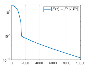
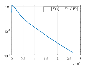
In this section, we use computational experiments to demonstrate the merits and the effectiveness of our approach for multi-block optimization problems. In each experiment, we apply the primal-dual gradient flow dynamics (17) to model instances (3b)-(6b) discussed in Section II-A, respectively. In Example 1, we apply distributed dynamics (25) to (3b). Even if the smooth component $f$ is not strongly convex in this case, since the nonsmooth block $g$ satisfies Assumption 3(i), Corollary 1 establishes Semi-GES of distributed dynamics (see Remark 3). In Example 2, even though there is not any smooth terms in (4b), Theorem 1 establish the GAS (see Remark 5). In Example 3, we demonstrate that our results are applicable to a more general setups such as (5) where constraint matrices are replaced by bounded linear operators. Corollary 1 can be applied to Examples 2 and 3 as well under certain constraint qualifications [57, Proposition 12] (see Remark 4). Finally, in Example 4, we demonstrate Semi-GES of dynamics (17) on (6b) where the nonsmooth block is not polyhedral but satisfies Assumption 3(ii). In all examples, we set $\alpha=1$ in (17) to illustrate conservatism of the stability analysis on the upper bound of the time constant (see Remark 7). We conduct our experiments on small-scale problems using Matlab’s function ode45 with relative and absolute tolerances $10^{-9}$ and $10^{-12}$, respectively.

Example 1: Decentralized lasso over a network. We consider decentralized problem (3) where each agent $i\in\{1,\cdots,10\}$ minimizes the sum of the following functions

$$f_{i}(\tilde{x})\,=\,(1/2)\|G_{i}\tilde{x}\,-\,h_{i}\|^{2},~{}~{}g_{i}(\tilde{x})\,=\,\tau_{i}\|\tilde{x}\|_{1}.$$

Following the problem setup given in [41], the data is generated as follows. Each measurement $h_{i}\in\mathbb{R}^{3}$ (known only by agent $i$) is constructed as $y_{i}=M_{i}\tilde{x}+\omega_{i}$ where entries of $M_{i}\in\mathbb{R}^{3\times 100}$ and $\omega_{i}\in\mathbb{R}^{3}$ are sampled from standard normal distribution and $M_{i}$ is normalized to $\|M_{i}\|=1$. Sparse signal $\tilde{x}\in\mathbb{R}^{100}$ has $5$ randomly chosen non-zero entries each of which is randomly drawn from $\{1,\ldots,5\}$. Regularization parameters $\{\tau_{i}\}_{i=1}^{10}$ are determined randomly to satisfy $\sum_{i=1}^{10}\tau_{i}=1.15$.

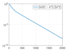
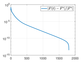
Dynamics (17) applied to (3b) takes the decentralized form of (25) where $\nabla f_{i}(x_{i})\,=\,G_{i}^{T}(G_{i}x_{i}\,+\,h_{i})$ and $\operatorname{\mathbf{prox}}_{\mu g_{i}}(z)$ is the shrinkage operator $\mathcal{S}_{1,\tau_{i}\mu}(z)$ whose $i$th entry is given by $[\mathcal{S}_{1,\mu}(z)]_{i}=\max\left(|z_{i}|-\mu,\ 0\right)\operatorname{sign}(z_{i})$. Lagrangian parameter $\mu$ is set to $1$ and the initial conditions are set to zero. The plots of relative state and function errors as well as topology of the network are given in Figure 1.

Refer to caption
network topology

relative state error

Refer to caption
time $t$

relative function error

Refer to caption
time $t$
Figure 1: Topology of the underlying communication network in distributed lasso problem (3) and the Semi-GES of the distributed dynamics (25). $F(t)$ denotes the objective value of (3b) at time $t$. The reference solution is obtained by using CVX.

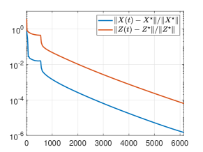
Example 2: Principle component pursuit. Following the problem setup given in [45], we generate the data for problem (4) as follows. Constraint matrix $Q\in\mathbb{R}^{200\times 200}$ is constructed as $Q=Q_{1}+Q_{2}+Q_{3}$. Here, $Q_{1}=R_{1}R_{2}^{T}$ where $R_{1}$ and $R_{2}$ are independent $200\times 10$ dimensional matrices whose entries are sampled from the standard normal distribution. The nonzero entries of binary mask $\Omega$ are determined at random and $80\%$ of all entries are set to $1$. The support of $Q_{2}$ is sampled uniformly among nonzero entries of $\Omega$ with sparsity ratio $5\%$ and the nonzero entries of $Q_{2}$ are uniformly sampled from interval $[-500\ 500]$. Lastly, $Q_{3}$ is modeled as a white Gaussian noise with standard deviation $\sigma=10^{-3}$. The remaining parameters are set to $\tau=1/\sqrt{200}$ and $\delta=\sqrt{200+\sqrt{1600}}\sigma$.

Dynamics (17) applied to (4b) take the following form

$\displaystyle\dot{\Lambda}$ $\displaystyle\!\!\!=\!\!\!$ $\displaystyle\alpha\,(Z_{1}\,+\,Z_{2}\,+\,Z_{3}\,-\,Q)$ (56a)
$\displaystyle\dot{Y}_{j}$ $\displaystyle\!\!\!=\!\!\!$ $\displaystyle\alpha(Z_{j}\,-\,\mathcal{S}_{j,\mu_{j}}(Z_{j}\,+\,\mu Y_{j})),\quad j\,=\,1,2,3$ (56b)
$\displaystyle\dot{Z}_{j}$ $\displaystyle\!\!\!=\!\!\!$ $\displaystyle-(Y_{j}\,+\,\tfrac{1}{\alpha\mu}\dot{Y}_{j})\,-\,(\Lambda\,+\,\tfrac{1}{\alpha\mu}\dot{\Lambda}),\quad j\,=\,1,2,3$ (56c)

where $(\mu_{1},\mu_{2},\mu_{3})=(\tau\mu,\mu,\delta)$. Here, $(i,j)$-entry of the output of shrinkage operator $\mathcal{S}_{1,\mu_{1}}$ is given by

$$\left[\mathcal{S}_{1,\mu}(X)\right]_{ij}\,=\,\max\left(|X_{ij}|\,-\,\mu,0\right)\operatorname{sign}(X_{ij}).$$ (57)

The proximal operator $\mathcal{S}_{2}$ of nuclear norm amounts to applying shrinkage operator $\mathcal{S}_{1}$ to the singular values, i.e.,

$$\mathcal{S}_{2,\mu}(X)\,=\,U\mathcal{S}_{1,\mu}(\Sigma)V^{T}$$ (58)

where $X=U\Sigma V^{T}$ is the singular value decomposition of $X$. Lastly, the proximal operator $\mathcal{S}_{3}$ of indicator function in (4a) is the projection operator

$$\mathcal{S}_{3,\mu}(X)\,=\,X\circ\Omega^{c}\,+\,\min(1,\,\mu/\|X\circ\Omega\|_{F})X\circ\Omega$$

where $\Omega_{ij}^{c}=1-\Omega_{ij}$ and $\circ$ denotes Hadamard product. Based on the formula given in [45], Lagrange penalty is set to $\mu=1.75$ and the initial conditions are chosen zero. The plots of relative state and function errors are given in Figure 2. As proven in Theorem 1 and demonstrated in Figure 2, PD gradient flow dynamics (17) converge even if the objective function does not include any smooth terms. We note that proximal gradient methods [70] cannot be used in this example because of the additional constraint on $Z_{3}$. The techniques based on multi-block ADMM such as VASALM [45] have convergence guarantees for only three blocks, whereas PD gradient flow dynamics (17) are globally convergent for arbitrary number of blocks.

relative state error

Refer to caption
time $t$

relative function error

Refer to caption
time $t$
Figure 2: Semi-GES of dynamics (56) for principle component pursuit problem (4). $F(t)$ denotes the objective value of (4b) at time $t$. The reference solution is obtained by performing $10^{4}$ iterations of VASALM algorithm [45].

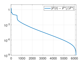
Example 3: Covariance completion. We use the mass-spring-damper example in [49] to generate problem data for model (5). The parameters $A,B,C,Q$, and $\gamma$ are generated by the script222https://www.ece.umn.edu/users/mihailo/software/ccama/run_ccama.html provided in [49] for $N=40$ masses. The dynamics (17) applied to (5b) take the form,

$\displaystyle\dot{\Lambda}_{1}$ $\displaystyle\!\!\!=\!\!\!$ $\displaystyle\alpha(\mathcal{E}_{1}(X)\,+\,Z)$ (59a)
$\displaystyle\dot{\Lambda}_{2}$ $\displaystyle\!\!\!=\!\!\!$ $\displaystyle\alpha(\mathcal{E}_{2}(X)\,-\,Q)$ (59b)
$\displaystyle\dot{Y}$ $\displaystyle\!\!\!=\!\!\!$ $\displaystyle\alpha(Z\,-\,\mathcal{S}_{2,\gamma\mu}(Z\,+\,\mu Y))$ (59c)
$\displaystyle\dot{Z}$ $\displaystyle\!\!\!=\!\!\!$ $\displaystyle-(Y\,+\,\tfrac{1}{\alpha\mu}\dot{Y})\,-\,(\Lambda_{1}+\tfrac{1}{\alpha\mu}\dot{\Lambda}_{1})$ (59d)
$\displaystyle\dot{X}$ $\displaystyle\!\!\!=\!\!\!$ $\displaystyle(X\,+\,\delta I)^{-1}\,-\,\mathcal{E}_{1}(\Lambda_{1}+\tfrac{1}{\alpha\mu}\dot{\Lambda}_{1})\,-\,\mathcal{E}_{2}(\Lambda_{2}+\tfrac{1}{\alpha\mu}\dot{\Lambda}_{2})$ (59e)

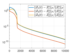
where the proximal operator of nuclear norm $\mathcal{S}_{2,\mu}$ is given in (58), $\mathcal{E}_{1}(X)=AX+XA^{T}$, and $\mathcal{E}_{2}(X)=(BXB^{T})\circ C$. We set $\mu=1$, $\delta=10^{-12}$ and the initial conditions are determined by the code script cited above as follows. For $Z(0)=Y(0)=\Lambda_{2}(0)=I\in\mathbb{R}^{N\times N}$, $X(0)$ is the solution of $\mathcal{E}_{1}(X)=-Z(0)$, and $\Lambda_{1}(0)=10\Lambda_{1}/\|\Lambda_{1}\|_{2}$ where $\Lambda_{1}$ is the solution of the Lyapunov equation $A^{T}\Lambda_{1}+\Lambda_{1}A=-X(0)$. The plots of relative state and function errors are given in Figure 3.

relative state error

Refer to caption
time $t$

relative function error

Refer to caption
time $t$
Figure 3: Semi-GES of dynamics (59) for covariance completion problem (5). $F(t)$ denotes the objective value of (5b) at time $t$. The reference solution is obtained by using CVX.

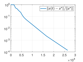
Example 4: Sparse group lasso. We consider the following problem as an instance of model (6)

$$\operatorname*{minimize}\limits_{x}~{}\tfrac{1}{2}\|q\,-\,Tx\|^{2}_{2}\,+\,\tau_{2}\|x\|_{1}\,+\,\tau_{2}\|x\|_{1,2}$$ (60)

which can be brought into the form of (1) as

$$\begin{array}[]{rcl}\operatorname*{minimize}\limits_{x,\,z}&\!\!\!\!\!\!&\tfrac{1}{2}\|x_{1}\|_{2}^{2}\,+\,\tau_{1}\|z_{1}\|_{1}\,+\,\tau_{2}\|z_{2}\|_{1,2}\\[2.84544pt] \operatorname*{subject~{}to}&\!\!\!\!\!\!&\left[\begin{array}[]{cc}I&T\\ 0&I\\ 0&I\end{array}\right]\left[\begin{array}[]{c}x_{1}\\ x_{2}\end{array}\right]\,+\,\left[\begin{array}[]{cc}0&0\\ -I&0\\ 0&-I\end{array}\right]\left[\begin{array}[]{c}z_{1}\\ z_{2}\end{array}\right]\,-\,\left[\begin{array}[]{c}q\\ 0\\ 0\end{array}\right]\,=\,0.\end{array}$$

Using the problem setup given in [54], we generate the data as follows. The entries of $T\in\mathbb{R}^{60\times 2000}$ are sampled from standard normal distribution and $q$ is constructed as q=(T1+T2+T3)\macc@depthΔ\frozen@everymath\macc@group\macc@set@skewchar\macc@nested@a111x+σω𝑞subscript𝑇1subscript𝑇2subscript𝑇3\macc@depthΔ\frozen@everymath\macc@group\macc@set@skewchar\macc@nested@a111𝑥𝜎𝜔q=(T_{1}+T_{2}+T_{3})\macc@depth\char 1\relax\frozen@everymath{\macc@group}\macc@set@skewchar\macc@nested@a 111{x}+\sigma\omega where $T=[T_{1}\cdots T_{50}]$ is a partition of columns, \macc@depthΔ\frozen@everymath\macc@group\macc@set@skewchar\macc@nested@a111x=[1 2 3 4 5 0 0]T30\macc@depthΔ\frozen@everymath\macc@group\macc@set@skewchar\macc@nested@a111𝑥superscriptdelimited-[]123450 0𝑇superscript30\macc@depth\char 1\relax\frozen@everymath{\macc@group}\macc@set@skewchar\macc@nested@a 111{x}=[1\,2\,3\,4\,5\,0\,\cdots\,0]^{T}\in\mathbb{R}^{30}, noise vector $\omega$ is sampled from standard normal distribution, and $\sigma$ is set so that the signal to noise ratio is $2$. Using the explicit formulas in [54], the remaining parameters are chosen as $\tau_{1}=114$ and $\tau_{2}=37.94$.

Dynamics (17) applied to above problem takes the following form

$\displaystyle\dot{\lambda}$ $\displaystyle\!\!\!=\!\!\!$ $\displaystyle\alpha\left(Ex\,+\,Fz\,-\,q\right)$ (61a)
$\displaystyle\left[\begin{array}[]{c}\dot{y}_{1}\\ \dot{y}_{2}\end{array}\right]$ $\displaystyle\!\!\!=\!\!\!$ $\displaystyle\alpha\big{(}\left[\begin{array}[]{c}z_{1}\\ z_{2}\end{array}\right]-\left[\begin{array}[]{c}\mathcal{S}_{1,\mu_{1}}(z_{1}\,+\,\mu y_{1})\\ \mathcal{S}_{4,\mu_{2}}(z_{2}\,+\,\mu y_{2})\end{array}\right]\big{)}$ (61h)
$\displaystyle\left[\begin{array}[]{c}\dot{z}_{1}\\ \dot{z}_{2}\end{array}\right]$ $\displaystyle\!\!\!=\!\!\!$ $\displaystyle\,-\,\left[\begin{array}[]{c}y_{1}\\ y_{2}\end{array}\right]\,-\,\tfrac{1}{\mu_{2}}\left[\begin{array}[]{c}\dot{y}_{1}\\ \dot{y}_{2}\end{array}\right]\,-\,F^{T}(\lambda\,+\,\tfrac{1}{\mu\alpha}\dot{\lambda})$ (61o)
$\displaystyle\left[\begin{array}[]{c}\dot{x}_{1}\\ \dot{x}_{2}\end{array}\right]$ $\displaystyle\!\!\!=\!\!\!$ $\displaystyle\,-\,\left[\begin{array}[]{c}x_{1}\\ 0\end{array}\right]\,-\,E^{T}(\lambda\,+\,\tfrac{1}{\mu\alpha}\dot{\lambda})$ (61t)

where $(\mu_{1},\mu_{2})=(\tau_{1}\mu,\tau_{2}\mu)$ and $\mathcal{S}_{1}$ is the shrinkage operator given in (57). Proximal operator $\mathcal{S}_{4}$ is the block-shrinkage defined as

$$\left[\mathcal{S}_{4,\mu}(z)\right)]_{h}\,=\,\max\left(0,\,1-\mu/\|[z]_{h}\|\right)[z]_{h}$$

for all $h\in\mathcal{I}$ where $z\in\mathbb{R}^{m}$ and $\mathcal{I}$ is the partition of $\{1,\ldots,m\}$ encoded in the $\ell_{1,2}$-norm. In our case, $\mathcal{I}$ is just uniform partition of $\{1,\ldots,2000\}$ to $50$ intervals each containing $40$ indices. Penalty parameter $\mu$ is taken $1$ and the initial conditions are chosen zero. The plots of relative state and function errors are given in Figure 4.

relative state error

Refer to caption
time $t$

relative function error

Refer to caption
time $t$
Figure 4: Semi-GES of dynamics (61) for sparse group lasso problem (60) (an instance of (6)). $F(t)$ denotes the objective value of (60) at time $t$. The reference solutions are obtained by using CVX.

VI Concluding remarks

We demonstrated the utility of employing gradient flow dynamics for solving composite optimization problems in which a convex objective function is given by a sum of multiple, possibly nonsmooth, terms subject to the generalized consensus constraint. We developed a systematic approach for solving classes of problems that can be brought into this form and identifed the weakest set of structural properties that allow us to establish exponentially fast convergence. In particular, we focused on primal-dual gradient flow dynamics resulting from the associated proximal augmented Lagrangian. Without making any smoothness, strong convexity, or rank assumptions, we first established the global asymptotic stability of the proposed dynamics. By restricting the class of nonsmooth terms in the objective function, we then proved local exponential stability, which, combined with our initial result, implies global exponential convergence. With the presence of smooth terms in the objective function and additional conditions on the constraint matrices, we proved global exponential stability without any additional restrictions on the nonsmooth components. We also showed that the conditions on the constraint matrices that we introduced are necessary for global exponential stability unless additional assumptions are made on the nonsmooth terms. We have provided several examples, including application to distributed optimization, to illustrate the merits and the effectiveness of our framework for solving a broad range of nonsmooth composite optimization problems.

References

  • [1] N. Parikh and S. Boyd, “Proximal algorithms,” Found. Trends Opt., vol. 1, no. 3, pp. 123–231, 2013.
  • [2] S. Boyd, N. Parikh, E. Chu, B. Peleato, and J. Eckstein, “Distributed optimization and statistical learning via the alternating direction method of multipliers,” Found. Trends Mach. Learn., vol. 3, no. 1, pp. 1–124, 2011.
  • [3] A. Chambolle and T. Pock, “A first-order primal-dual algorithm for convex problems with applications to imaging,” J. Math. Imaging Vision, vol. 40, pp. 120–145, 2011.
  • [4] P. L. Combettes and J. Pesquet, “Primal-dual splitting algorithm for solving inclusions with mixtures of composite, Lipschitzian, and parallel-sum type monotone operators,” Set-Valued Var. Anal., vol. 20, no. 2, pp. 307–330, 2012.
  • [5] L. Condat, “A primal–dual splitting method for convex optimization involving Lipschitzian, proximable and linear composite terms,” J. Optim. Theory Appl., vol. 158, no. 2, pp. 460–479, 2013.
  • [6] D. Davis and W. Yin, “A three-operator splitting scheme and its optimization applications,” Set-Valued Var. Anal., vol. 25, pp. 829–858, 2017.
  • [7] P. Latafat and P. Patrinos, “Asymmetric forward–backward–adjoint splitting for solving monotone inclusions involving three operators,” Comput. Optim. Appl., vol. 68, pp. 57–93, 2017.
  • [8] W. Deng and W. Yin, “On the global and linear convergence of the generalized alternating direction method of multipliers,” J. Sci. Comput., vol. 66, no. 3, pp. 889–916, 2016.
  • [9] C. Chen, B. He, Y. Ye, and X. Yuan, “The direct extension of ADMM for multi-block convex minimization problems is not necessarily convergent,” Math. Program., vol. 155, no. 1, pp. 57–79, 2016.
  • [10] S. Ma, “Alternating proximal gradient method for convex minimization,” J. Sci. Comput., vol. 68, no. 2, pp. 546–572, 2016.
  • [11] D. Bertsekas and J. Tsitsiklis, Parallel and Distributed Computation: Numerical Methods.   Nashua, NH: Athena Scientific, 2015.
  • [12] W. Deng, M. Lai, Z. Peng, and W. Yin, “Parallel multi-block ADMM with O(1/k) convergence,” J. Sci. Comput., vol. 71, no. 2, pp. 712–736, 2017.
  • [13] B. He, L. Hou, and X. Yuan, “On full Jacobian decomposition of the augmented Lagrangian method for separable convex programming,” SIAM J. Optim., vol. 25, no. 4, pp. 2274–2312, 2015.
  • [14] B. He, M. Tao, and X. Yuan, “Alternating direction method with Gaussian back substitution for separable convex programming,” SIAM J. Optim., vol. 22, no. 2, pp. 313–340, 2012.
  • [15] T. Lin, S. Ma, and S. Zhang, “Iteration complexity analysis of multi-block ADMM for a family of convex minimization without strong convexity,” J. Sci. Comput., vol. 69, no. 1, pp. 52–81, 2016.
  • [16] K. J. Arrow, L. Hurwicz, and H. Uzawa, Studies in Linear and Non-linear Programming.   Palo Alto, CA: Stanford Univ. Press, 1958.
  • [17] D. Feijer and F. Paganini, “Stability of primal–dual gradient dynamics and applications to network optimization,” Automatica J. IFAC, vol. 46, no. 12, pp. 1974–1981, 2010.
  • [18] A. Cherukuri, E. Mallada, and J. Cortes, “Asymptotic convergence of constrained primal-dual dynamics,” Systems Control Lett., vol. 87, pp. 10–15, 2016.
  • [19] A. Cherukuri, B. Gharesifard, and J. Cortes, “Saddle-point dynamics: conditions for asymptotic stability of saddle points,” SIAM J. Control Optim., vol. 55, no. 1, pp. 486–511, 2017.
  • [20] A. Cherukuri, E. Mallada, S. Low, and J. Cortes, “The role of convexity on saddle-point dynamics: Lyapunov function and robustness,” IEEE Trans. Automat. Control, vol. 63, no. 8, pp. 2449–2464, 2018.
  • [21] T. Holding and I. Lestas, “On the convergence to saddle points of concave-convex functions, the gradient method and emergence of oscillations,” in Proc. IEEE Conf. Decis. Control, 2014, pp. 1143–1148.
  • [22] G. Qu and N. Li, “On the exponential stability of primal-dual gradient dynamics,” IEEE Control Syst. Lett., vol. 3, no. 1, pp. 43–48, 2018.
  • [23] J. Cortes and S. K. Niederlander, “Distributed coordination for nonsmooth convex optimization via saddle-point dynamics,” J. Nonlinear Sci., vol. 29, no. 4, pp. 1247–1272, 2019.
  • [24] X. Chen and N. Li, “Exponential stability of primal-dual gradient dynamics with non-strong convexity,” in Proc. Amer. Control Conf.   IEEE, 2020, pp. 1612–1618.
  • [25] I. K. Ozaslan and M. R. Jovanović, “On the global exponential stability of primal-dual dynamics for convex problems with linear equality constraints,” in Proc. Amer. Control Conf., 2023.
  • [26] I. K. Ozaslan and M. R. Jovanović, “Tight lower bounds on the convergence rate of primal-dual dynamics for equality constrained convex problems,” in Proc. IEEE Conf. Decis. Control, 2023, pp. 7318–7323.
  • [27] D. Ding, B. Hu, N. K. Dhingra, and M. R. Jovanović, “An exponentially convergent primal-dual algorithm for nonsmooth composite minimization,” in Proc. IEEE Conf. Decis. Control, 2018, pp. 4927–4932.
  • [28] N. K. Dhingra, S. Z. Khong, and M. R. Jovanović, “The proximal augmented Lagrangian method for nonsmooth composite optimization,” IEEE Trans. Automat. Control, vol. 64, no. 7, pp. 2861–2868, 2019.
  • [29] I. K. Ozaslan, S. Hassan-Moghaddam, and M. R. Jovanović, “On the asymptotic stability of proximal algorithms for convex optimization problems with multiple non-smooth regularizers,” in Proc. Amer. Control Conf., 2022.
  • [30] I. K. Ozaslan and M. R. Jovanović, “Exponential convergence of primal-dual dynamics for multi-block problems under local error bound condition,” in Proc. IEEE Conf. Decis. Control, 2022, pp. 7579–7584.
  • [31] D. Ding and M. R. Jovanović, “Global exponential stability of primal-dual gradient flow dynamics based on the proximal augmented Lagrangian: A Lyapunov-based approach,” in Proc. IEEE Conf. Decis. Control, 2020, pp. 4836–4841.
  • [32] Y. Tang, G. Qu, and N. Li, “Semi-global exponential stability of augmented primal–dual gradient dynamics for constrained convex optimization,” Systems Control Lett., vol. 144, p. 104754, 2020.
  • [33] H. D. Nguyen, T. L. Vu, K. Turitsyn, and J. Slotine, “Contraction and robustness of continuous time primal-dual dynamics,” IEEE Contr. Syst. Lett., vol. 2, no. 4, pp. 755–760, Oct. 2018.
  • [34] P. Cisneros-Velarde, S. Jafarpour, and F. Bullo, “A contraction analysis of primal-dual dynamics in distributed and time-varying implementations,” IEEE Trans. Autom. Control, vol. 67, no. 7, pp. 3560–3566, 2022.
  • [35] A. Davydov, V. Centorrino, A. Gokhale, G. Russo, and F. Bullo, “Contracting dynamics for time-varying convex optimization,” arXiv:2305.15595, 2023.
  • [36] H. Attouch, Z. Chbani, J. Fadili, and H. Riahi, “Fast convergence of dynamical ADMM via time scaling of damped inertial dynamics,” J. Optim. Theory Appl., vol. 193, no. 1, pp. 704–736, 2022.
  • [37] X. Zeng, J. Lei, and J. Chen, “Dynamical primal-dual Nesterov accelerated method and its application to network optimization,” IEEE Trans. Automat. Control, vol. 68, no. 3, pp. 1760–1767, 2023.
  • [38] X. He, R. Hu, and Y. Fang, ““Second-order primal”+“first-order dual” dynamical systems with time scaling for linear equality constrained convex optimization problems,” IEEE Trans. Automat. Control, vol. 67, no. 8, pp. 4377–4383, 2022.
  • [39] N. K. Dhingra, S. Z. Khong, and M. R. Jovanović, “A second order primal-dual method for nonsmooth convex composite optimization,” IEEE Trans. Automat. Control, vol. 67, no. 8, pp. 4061–4076, 2022.
  • [40] W. Shi, Q. Ling, G. Wu, and W. Yin, “EXTRA: An exact first-order algorithm for decentralized consensus optimization,” SIAM J. Optim., vol. 25, no. 2, pp. 944–966, 2015.
  • [41] W. Shi, Q. Ling, G. Wu, and W. Yin, “A proximal gradient algorithm for decentralized composite optimization,” IEEE Trans. Signal Process., vol. 63, no. 22, pp. 6013–6023, 2015.
  • [42] S. Sastry, Nonlinear Systems: Analysis, Stability, and Control.   Berlin: Springer Science & Business Media, 2013, vol. 10.
  • [43] C. Zhao, U. Topcu, N. Li, and S. Low, “Design and stability of load-side primary frequency control in power systems,” IEEE Trans. Automat. Control, vol. 59, no. 5, pp. 1177–1189, 2014.
  • [44] B. Johansson, “On distributed optimization in networked systems,” Ph.D. dissertation, KTH, 2008.
  • [45] M. Tao and X. Yuan, “Recovering low-rank and sparse components of matrices from incomplete and noisy observations,” SIAM J. Optim., vol. 21, no. 1, pp. 57–81, 2011.
  • [46] Z. Zhou, X. Li, J. Wright, E. Candes, and Y. Ma, “Stable principal component pursuit,” in IEEE Int. Symp. Inf. Theor. Proc.   IEEE, 2010, pp. 1518–1522.
  • [47] V. Chandrasekaran, P. A. Parrilo, and A. S. Willsky, “Latent variable graphical model selection via convex optimization,” Ann. Statist., vol. 40, no. 4, pp. 1610–1613, 2012.
  • [48] Y. Peng, A. Ganesh, J. Wright, W. Xu, and Y. Ma, “RASL: Robust alignment by sparse and low-rank decomposition for linearly correlated images,” IEEE Trans. Pattern Anal. Mach. Intell., vol. 34, no. 11, pp. 2233–2246, 2012.
  • [49] A. Zare, Y. Chen, M. R. Jovanović, and T. T. Georgiou, “Low-complexity modeling of partially available second-order statistics: theory and an efficient matrix completion algorithm,” IEEE Trans. Automat. Control, vol. 62, no. 3, pp. 1368–1383, 2017.
  • [50] A. Zare, M. R. Jovanović, and T. T. Georgiou, “Colour of turbulence,” J. Fluid Mech., vol. 812, pp. 636–680, 2017.
  • [51] A. Zare, T. T. Georgiou, and M. R. Jovanović, “Stochastic dynamical modeling of turbulent flows,” Annu. Rev. Control Robot. Auton. Syst., vol. 3, pp. 195–219, 2020.
  • [52] M. Pilanci and T. Ergen, “Neural networks are convex regularizers: Exact polynomial-time convex optimization formulations for two-layer networks,” in Proc. Int. Conf. Mach. Learn., 2020, pp. 7695–7705.
  • [53] Y. Bai, T. Gautam, and S. Sojoudi, “Efficient global optimization of two-layer relu networks: Quadratic-time algorithms and adversarial training,” SIAM J. Math. Data Sci., vol. 5, no. 2, pp. 446–474, 2023.
  • [54] N. Simon, J. Friedman, T. Hastie, and R. Tibshirani, “A sparse-group lasso,” J. Comput. Graph. Statist., vol. 22, no. 2, pp. 231–245, 2013.
  • [55] H. H. Bauschke and P. L. Combettes, Convex Analysis and Monotone Operator Theory in Hilbert Spaces.   Switzerland: Springer, 2011.
  • [56] S. Bubeck, “Convex optimization: Algorithms and complexity,” Found. Trends Mach. Learn., vol. 8, no. 3-4, pp. 231–357, 2015.
  • [57] Z. Zhou and A. So, “A unified approach to error bounds for structured convex optimization problems,” Math. Program., vol. 165, no. 2, pp. 689–728, 2017.
  • [58] R. T. Rockafellar, “New applications of duality in nonlinear programming,” in Proc. Conf. Prob. Theory, 1971, pp. 73–81.
  • [59] P. Lions and B. Mercier, “Splitting algorithms for the sum of two nonlinear operators,” SIAM J. Numer. Anal., vol. 16, no. 6, pp. 964–979, 1979.
  • [60] R. Nishihara, L. Lessard, B. Recht, A. Packard, and M. Jordan, “A general analysis of the convergence of ADMM,” in Proc. Int. Conf. Mach. Learn.   PMLR, 2015, pp. 343–352.
  • [61] P. Giselsson and S. Boyd, “Linear convergence and metric selection for Douglas-Rachford splitting and ADMM,” IEEE Trans. Automat. Control, vol. 62, no. 2, pp. 532–544, 2016.
  • [62] T. Lin, S. Ma, and S. Zhang, “On the global linear convergence of the ADMM with multiblock variables,” SIAM J. Optim., vol. 25, no. 3, pp. 1478–1497, 2015.
  • [63] M. Hong and Z. Luo, “On the linear convergence of the alternating direction method of multipliers,” Math. Program., vol. 162, no. 1, pp. 165–199, 2017.
  • [64] A. J. Hoffman, “On approximate solutions of systems of linear inequalities,” J. Res. Natl. Bur. Stand. (U. S.), vol. 49, pp. 263–265, 1952.
  • [65] W. Shi, Q. Ling, K. Yuan, G. Wu, and W. Yin, “On the linear convergence of the ADMM in decentralized consensus optimization,” IEEE Trans. Signal Process., vol. 62, no. 7, pp. 1750–1761, 2014.
  • [66] P. Latafat, L. Stella, and P. Patrinos, “New primal-dual proximal algorithm for distributed optimization,” in Proc. IEEE Conf. Decis. Control, 2016, pp. 1959–1964.
  • [67] R. T. Rockafellar and R. Wets, Variational Analysis.   Berlin: Springer, 2009, vol. 317.
  • [68] H. K. Khalil, Nonlinear Systems.   Hoboken, NY: Patience Hall, 2002, vol. 115.
  • [69] H. Karimi, J. Nutini, and M. Schmidt, “Linear convergence of gradient and proximal-gradient methods under the Polyak-Lojasiewicz condition,” in Joint Eur. Conf. Mach. Learn. Knowl. Discov. Data., 2016, pp. 795–811.
  • [70] Z. Lin, A. Ganesh, J. Wright, L. Wu, M. Chen, and Y. Ma, “Fast convex optimization algorithms for exact recovery of a corrupted low-rank matrix,” Coordinated Science Laboratory Report no. UILU-ENG-09-2214, DC-246, 2009.
  • [71] Z. Luo and P. Tseng, “On the linear convergence of descent methods for convex essentially smooth minimization,” SIAM J. Control Optim., vol. 30, no. 2, pp. 408–425, 1992.
  • [72] P. Tseng, “Approximation accuracy, gradient methods, and error bound for structured convex optimization,” Math. Program., vol. 125, no. 2, pp. 263–295, 2010.
  • [73] P. Tseng and S. Yun, “A coordinate gradient descent method for nonsmooth separable minimization,” Math. Program., vol. 117, pp. 387–423, 2009.

-A Proof of Lemma 1

Lemma 1

Let Assumption 1 hold. The time derivative of $V_{1}$ in (26) along the solutions of primal-dual gradient flow dynamics (17) with $\alpha>0$ satisfies

$$\dot{V}_{1}(t)\,\leq\,-\tfrac{\alpha}{\max(L_{f},\,\mu)}\big{(}\|\nabla f(x(t))\,-\,\nabla f(x^{\star})\|^{2}\,+\,\|\nabla_{y}\mathcal{L}_{\mu}(x(t),z(t);y(t),\lambda(t))\|^{2}\,+\,\|\nabla_{\lambda}\mathcal{L}_{\mu}(x(t),z(t);y(t),\lambda(t))\|^{2}\big{)}$$

where $L_{f}$ is the Lipschitz constant of $\nabla f$.

Proof:

Let $\tilde{x}\mathrel{\mathop{:}}=x-x^{\star}$, $\tilde{z}\mathrel{\mathop{:}}=z-z^{\star}$, $\tilde{y}\mathrel{\mathop{:}}=y-y^{\star}$, $\tilde{\lambda}\mathrel{\mathop{:}}=\lambda-\lambda^{\star}$, and $\widetilde{w}\mathrel{\mathop{:}}=\operatorname{\mathbf{prox}}_{\mu g}(z+\mu y)-\operatorname{\mathbf{prox}}_{\mu g}(z^{\star}+\mu y^{\star})$, using the chain rule, the time derivative of $V_{1}$ can be written as

$\displaystyle\dot{V}_{1}$ $\displaystyle\,=\,\alpha\langle\dot{x},\tilde{x}\rangle\,+\,\alpha\langle\dot{z},\tilde{z}\rangle\,+\,\langle\dot{y},\tilde{y}\rangle\,+\,\langle\dot{\lambda},\tilde{\lambda}\rangle$
$\displaystyle\,=\,-\,\alpha\langle\nabla f(x)-\nabla f(x^{\star})\,+\,E^{T}(\tilde{\lambda}\,+\,\tfrac{1}{\alpha\mu}\dot{\lambda}),\tilde{x}\rangle\,-\,\alpha\langle\tilde{y}\,+\,\tfrac{1}{\alpha\mu}\dot{y}\,+\,F^{T}(\tilde{\lambda}\,+\,\tfrac{1}{\alpha\mu}\dot{\lambda},\tilde{z}\rangle\,+\,$
$\displaystyle\,\phantom{=}\,\phantom{-}\,\alpha\langle\tilde{z}\,-\,\widetilde{w},\tilde{y}\rangle\,+\,\alpha\langle E\tilde{x}\,+\,F\tilde{z},\tilde{\lambda}\rangle$
$\displaystyle\,=\,-\,\alpha\langle\nabla f(x)-\nabla f(x^{\star}),\tilde{x}\rangle\,-\,\tfrac{1}{\mu}\langle\dot{\lambda},E\tilde{x}\,+\,F\tilde{z}\rangle\,-\,\tfrac{1}{\mu}\langle\dot{y},\tilde{z}\rangle\,-\,\alpha\langle\widetilde{w},\tilde{y}\rangle$
$\displaystyle\,=\,-\,\alpha\langle\nabla f(x)-\nabla f(x^{\star}),\tilde{x}\rangle\,-\,\tfrac{\alpha}{\mu}\|E\tilde{x}\,+\,F\tilde{z}\|^{2}\,-\,\tfrac{\alpha}{\mu}(\langle\tilde{z}-\widetilde{w},\tilde{z}\rangle\,+\,\langle\widetilde{w},\mu\tilde{y}\rangle)$
$\displaystyle\,=\,-\,\alpha\langle\nabla f(x)-\nabla f(x^{\star}),\tilde{x}\rangle\,-\,\tfrac{\alpha}{\mu}\|E\tilde{x}\,+\,F\tilde{z}\|^{2}\,-\,\tfrac{\alpha}{\mu}(\|\tilde{z}\|^{2}\,-\,2\langle\widetilde{w},\tilde{z}\rangle\,+\,\langle\widetilde{w},\tilde{z}\,+\,\mu\tilde{y}\rangle)$ (62)

where the second equality follows from the fact that dynamics (17) are zero at any solutions satisfying (12), the third equality follows from the symmetry of inner products, the forth equality follows from (17c) and (17d), and the last equality follows from the linearity of inner products. Since the proximal operator is firmly non-expansive, we can bound $\dot{V}_{1}$ as

$$\begin{array}[]{rcl}\dot{V}_{1}&\!\!\!\leq\!\!\!&-\,\alpha\langle\nabla f(x)-\nabla f(x^{\star}),\tilde{x}\rangle\,-\,\tfrac{\alpha}{\mu}\|E\tilde{x}\,+\,F\tilde{z}\|^{2}\,-\,\tfrac{\alpha}{\mu}(\|\tilde{z}\|^{2}\,-\,2\langle\widetilde{w},\tilde{z}\rangle\,+\,\|\widetilde{w}\|^{2})\\[2.84544pt] &\!\!\!\leq\!\!\!&-\,\tfrac{\alpha}{L_{f}}\|\nabla f(x)-\nabla f(x^{\star})\|^{2}\,-\,\tfrac{\alpha}{\mu}\|E\tilde{x}\,+\,F\tilde{z}\|^{2}\,-\,\tfrac{\alpha}{\mu}\|\tilde{z}\,-\,\widetilde{w}\|^{2}\end{array}$$

where the second line is obtained by using the $L_{f}$-Lipschitz continuity of $\nabla f$. Rearrangement of terms completes the proof. ∎

-B Proof of Lemma 2

Lemma 2

The gradient of the dual function $d(y,\lambda)$,

d(y,λ)=[yd(y,λ)λd(y,λ)]=[\macc@depthΔ\frozen@everymath\macc@group\macc@set@skewchar\macc@nested@a111z(y,λ)𝐩𝐫𝐨𝐱μg(\macc@depthΔ\frozen@everymath\macc@group\macc@set@skewchar\macc@nested@a111z(y,λ)+μy)E\macc@depthΔ\frozen@everymath\macc@group\macc@set@skewchar\macc@nested@a111x(y,λ)+F\macc@depthΔ\frozen@everymath\macc@group\macc@set@skewchar\macc@nested@a111z(y,λ)q]𝑑𝑦𝜆delimited-[]subscript𝑦𝑑𝑦𝜆subscript𝜆𝑑𝑦𝜆delimited-[]\macc@depthΔ\frozen@everymath\macc@group\macc@set@skewchar\macc@nested@a111𝑧𝑦𝜆subscript𝐩𝐫𝐨𝐱𝜇𝑔\macc@depthΔ\frozen@everymath\macc@group\macc@set@skewchar\macc@nested@a111𝑧𝑦𝜆𝜇𝑦𝐸\macc@depthΔ\frozen@everymath\macc@group\macc@set@skewchar\macc@nested@a111𝑥𝑦𝜆𝐹\macc@depthΔ\frozen@everymath\macc@group\macc@set@skewchar\macc@nested@a111𝑧𝑦𝜆𝑞\nabla d(y,\lambda)\,=\,\left[\begin{array}[]{c}\nabla_{y}d(y,\lambda)\\ \nabla_{\lambda}d(y,\lambda)\end{array}\right]\,=\,\left[\begin{array}[]{c}\macc@depth\char 1\relax\frozen@everymath{\macc@group}\macc@set@skewchar\macc@nested@a 111{z}(y,\lambda)\,-\,\operatorname{\mathbf{prox}}_{\mu g}(\macc@depth\char 1\relax\frozen@everymath{\macc@group}\macc@set@skewchar\macc@nested@a 111{z}(y,\lambda)\,+\,\mu y)\\ E\macc@depth\char 1\relax\frozen@everymath{\macc@group}\macc@set@skewchar\macc@nested@a 111{x}(y,\lambda)\,+\,F\macc@depth\char 1\relax\frozen@everymath{\macc@group}\macc@set@skewchar\macc@nested@a 111{z}(y,\lambda)\,-\,q\end{array}\right]

is Lipschitz continuous with modulus $\mu$, where (\macc@depthΔ\frozen@everymath\macc@group\macc@set@skewchar\macc@nested@a111x,\macc@depthΔ\frozen@everymath\macc@group\macc@set@skewchar\macc@nested@a111z)\macc@depthΔ\frozen@everymath\macc@group\macc@set@skewchar\macc@nested@a111𝑥\macc@depthΔ\frozen@everymath\macc@group\macc@set@skewchar\macc@nested@a111𝑧(\macc@depth\char 1\relax\frozen@everymath{\macc@group}\macc@set@skewchar\macc@nested@a 111{x},\macc@depth\char 1\relax\frozen@everymath{\macc@group}\macc@set@skewchar\macc@nested@a 111{z}) denotes a $(y,\lambda)$-parameterized solution to (30).

Proof:

We first show that quantities $Ex+Fz-b$ and $z-\operatorname{\mathbf{prox}}_{\mu g}(z+\mu y)$ remain constant over the set of solutions to (30) at $(y,\lambda)$. Let (\macc@depthΔ\frozen@everymath\macc@group\macc@set@skewchar\macc@nested@a111x,\macc@depthΔ\frozen@everymath\macc@group\macc@set@skewchar\macc@nested@a111z)\macc@depthΔ\frozen@everymath\macc@group\macc@set@skewchar\macc@nested@a111𝑥\macc@depthΔ\frozen@everymath\macc@group\macc@set@skewchar\macc@nested@a111𝑧(\macc@depth\char 1\relax\frozen@everymath{\macc@group}\macc@set@skewchar\macc@nested@a 111{x},\macc@depth\char 1\relax\frozen@everymath{\macc@group}\macc@set@skewchar\macc@nested@a 111{z}) and (\macc@depthΔ\frozen@everymath\macc@group\macc@set@skewchar\macc@nested@a111x,\macc@depthΔ\frozen@everymath\macc@group\macc@set@skewchar\macc@nested@a111z)\macc@depthΔ\frozen@everymath\macc@group\macc@set@skewchar\macc@nested@a111superscript𝑥\macc@depthΔ\frozen@everymath\macc@group\macc@set@skewchar\macc@nested@a111superscript𝑧(\macc@depth\char 1\relax\frozen@everymath{\macc@group}\macc@set@skewchar\macc@nested@a 111{x}^{\prime},\macc@depth\char 1\relax\frozen@everymath{\macc@group}\macc@set@skewchar\macc@nested@a 111{z}^{\prime}) be two different solutions to (30) at $(y,\lambda)$. Let \macc@depthΔ\frozen@everymath\macc@group\macc@set@skewchar\macc@nested@a111w:=𝐩𝐫𝐨𝐱μg(\macc@depthΔ\frozen@everymath\macc@group\macc@set@skewchar\macc@nested@a111z+μy)\macc@depth\char 1\relax\frozen@everymath{\macc@group}\macc@set@skewchar\macc@nested@a 111{w}\mathrel{\mathop{:}}=\operatorname{\mathbf{prox}}_{\mu g}(\macc@depth\char 1\relax\frozen@everymath{\macc@group}\macc@set@skewchar\macc@nested@a 111{z}+\mu y) and \macc@depthΔ\frozen@everymath\macc@group\macc@set@skewchar\macc@nested@a111w:=𝐩𝐫𝐨𝐱μg(\macc@depthΔ\frozen@everymath\macc@group\macc@set@skewchar\macc@nested@a111z+μy)\macc@depth\char 1\relax\frozen@everymath{\macc@group}\macc@set@skewchar\macc@nested@a 111{w}^{\prime}\mathrel{\mathop{:}}=\operatorname{\mathbf{prox}}_{\mu g}(\macc@depth\char 1\relax\frozen@everymath{\macc@group}\macc@set@skewchar\macc@nested@a 111{z}^{\prime}+\mu y). Suppose, for contradiction, that either E\macc@depthΔ\frozen@everymath\macc@group\macc@set@skewchar\macc@nested@a111x+F\macc@depthΔ\frozen@everymath\macc@group\macc@set@skewchar\macc@nested@a111zE\macc@depthΔ\frozen@everymath\macc@group\macc@set@skewchar\macc@nested@a111x+F\macc@depthΔ\frozen@everymath\macc@group\macc@set@skewchar\macc@nested@a111z𝐸\macc@depthΔ\frozen@everymath\macc@group\macc@set@skewchar\macc@nested@a111𝑥𝐹\macc@depthΔ\frozen@everymath\macc@group\macc@set@skewchar\macc@nested@a111𝑧𝐸\macc@depthΔ\frozen@everymath\macc@group\macc@set@skewchar\macc@nested@a111superscript𝑥𝐹\macc@depthΔ\frozen@everymath\macc@group\macc@set@skewchar\macc@nested@a111superscript𝑧E\macc@depth\char 1\relax\frozen@everymath{\macc@group}\macc@set@skewchar\macc@nested@a 111{x}+F\macc@depth\char 1\relax\frozen@everymath{\macc@group}\macc@set@skewchar\macc@nested@a 111{z}\neq E\macc@depth\char 1\relax\frozen@everymath{\macc@group}\macc@set@skewchar\macc@nested@a 111{x}^{\prime}+F\macc@depth\char 1\relax\frozen@everymath{\macc@group}\macc@set@skewchar\macc@nested@a 111{z}^{\prime} or \macc@depthΔ\frozen@everymath\macc@group\macc@set@skewchar\macc@nested@a111z\macc@depthΔ\frozen@everymath\macc@group\macc@set@skewchar\macc@nested@a111w\macc@depthΔ\frozen@everymath\macc@group\macc@set@skewchar\macc@nested@a111z\macc@depthΔ\frozen@everymath\macc@group\macc@set@skewchar\macc@nested@a111w\macc@depthΔ\frozen@everymath\macc@group\macc@set@skewchar\macc@nested@a111𝑧\macc@depthΔ\frozen@everymath\macc@group\macc@set@skewchar\macc@nested@a111𝑤\macc@depthΔ\frozen@everymath\macc@group\macc@set@skewchar\macc@nested@a111superscript𝑧\macc@depthΔ\frozen@everymath\macc@group\macc@set@skewchar\macc@nested@a111superscript𝑤\macc@depth\char 1\relax\frozen@everymath{\macc@group}\macc@set@skewchar\macc@nested@a 111{z}-\macc@depth\char 1\relax\frozen@everymath{\macc@group}\macc@set@skewchar\macc@nested@a 111{w}\neq\macc@depth\char 1\relax\frozen@everymath{\macc@group}\macc@set@skewchar\macc@nested@a 111{z}^{\prime}-\macc@depth\char 1\relax\frozen@everymath{\macc@group}\macc@set@skewchar\macc@nested@a 111{w}^{\prime}. Since the augmented Lagrangian (14) is a convex function over the primal variables, set of its minimizers is also convex, which means that (x^,z^,w^)=((\macc@depthΔ\frozen@everymath\macc@group\macc@set@skewchar\macc@nested@a111x+\macc@depthΔ\frozen@everymath\macc@group\macc@set@skewchar\macc@nested@a111x)/2,(\macc@depthΔ\frozen@everymath\macc@group\macc@set@skewchar\macc@nested@a111z+\macc@depthΔ\frozen@everymath\macc@group\macc@set@skewchar\macc@nested@a111z)/2,(\macc@depthΔ\frozen@everymath\macc@group\macc@set@skewchar\macc@nested@a111w+\macc@depthΔ\frozen@everymath\macc@group\macc@set@skewchar\macc@nested@a111w)/2)^𝑥^𝑧^𝑤\macc@depthΔ\frozen@everymath\macc@group\macc@set@skewchar\macc@nested@a111𝑥\macc@depthΔ\frozen@everymath\macc@group\macc@set@skewchar\macc@nested@a111superscript𝑥2\macc@depthΔ\frozen@everymath\macc@group\macc@set@skewchar\macc@nested@a111𝑧\macc@depthΔ\frozen@everymath\macc@group\macc@set@skewchar\macc@nested@a111superscript𝑧2\macc@depthΔ\frozen@everymath\macc@group\macc@set@skewchar\macc@nested@a111𝑤\macc@depthΔ\frozen@everymath\macc@group\macc@set@skewchar\macc@nested@a111superscript𝑤2(\widehat{x},\widehat{z},\widehat{w})=((\macc@depth\char 1\relax\frozen@everymath{\macc@group}\macc@set@skewchar\macc@nested@a 111{x}\,+\,\macc@depth\char 1\relax\frozen@everymath{\macc@group}\macc@set@skewchar\macc@nested@a 111{x}^{\prime})/2,(\macc@depth\char 1\relax\frozen@everymath{\macc@group}\macc@set@skewchar\macc@nested@a 111{z}\,+\,\macc@depth\char 1\relax\frozen@everymath{\macc@group}\macc@set@skewchar\macc@nested@a 111{z}^{\prime})/2,(\macc@depth\char 1\relax\frozen@everymath{\macc@group}\macc@set@skewchar\macc@nested@a 111{w}\,+\,\macc@depth\char 1\relax\frozen@everymath{\macc@group}\macc@set@skewchar\macc@nested@a 111{w}^{\prime})/2) is also a minimizer. Moreover, Lagrangian (11) is a convex function over the primal variable; hence,

12((\macc@depthΔ\frozen@everymath\macc@group\macc@set@skewchar\macc@nested@a111x,\macc@depthΔ\frozen@everymath\macc@group\macc@set@skewchar\macc@nested@a111z,\macc@depthΔ\frozen@everymath\macc@group\macc@set@skewchar\macc@nested@a111w;y,λ)+(\macc@depthΔ\frozen@everymath\macc@group\macc@set@skewchar\macc@nested@a111x,\macc@depthΔ\frozen@everymath\macc@group\macc@set@skewchar\macc@nested@a111z,\macc@depthΔ\frozen@everymath\macc@group\macc@set@skewchar\macc@nested@a111w;y,λ))(x^,z^,w^;y,λ).12\macc@depthΔ\frozen@everymath\macc@group\macc@set@skewchar\macc@nested@a111𝑥\macc@depthΔ\frozen@everymath\macc@group\macc@set@skewchar\macc@nested@a111𝑧\macc@depthΔ\frozen@everymath\macc@group\macc@set@skewchar\macc@nested@a111𝑤𝑦𝜆\macc@depthΔ\frozen@everymath\macc@group\macc@set@skewchar\macc@nested@a111superscript𝑥\macc@depthΔ\frozen@everymath\macc@group\macc@set@skewchar\macc@nested@a111superscript𝑧\macc@depthΔ\frozen@everymath\macc@group\macc@set@skewchar\macc@nested@a111superscript𝑤𝑦𝜆^𝑥^𝑧^𝑤𝑦𝜆\tfrac{1}{2}(\mathcal{L}(\macc@depth\char 1\relax\frozen@everymath{\macc@group}\macc@set@skewchar\macc@nested@a 111{x},\macc@depth\char 1\relax\frozen@everymath{\macc@group}\macc@set@skewchar\macc@nested@a 111{z},\macc@depth\char 1\relax\frozen@everymath{\macc@group}\macc@set@skewchar\macc@nested@a 111{w};y,\lambda)\,+\,\mathcal{L}(\macc@depth\char 1\relax\frozen@everymath{\macc@group}\macc@set@skewchar\macc@nested@a 111{x}^{\prime},\macc@depth\char 1\relax\frozen@everymath{\macc@group}\macc@set@skewchar\macc@nested@a 111{z}^{\prime},\macc@depth\char 1\relax\frozen@everymath{\macc@group}\macc@set@skewchar\macc@nested@a 111{w}^{\prime};y,\lambda))\,\geq\,\mathcal{L}(\widehat{x},\widehat{z},\widehat{w};y,\lambda). (63)

Since $\|\cdot\|^{2}$ is a strongly convex function and the arguments are not equal by the initial supposition, we have the following inequalities with at least one of them being strict

12(E\macc@depthΔ\frozen@everymath\macc@group\macc@set@skewchar\macc@nested@a111x+F\macc@depthΔ\frozen@everymath\macc@group\macc@set@skewchar\macc@nested@a111zb2+E\macc@depthΔ\frozen@everymath\macc@group\macc@set@skewchar\macc@nested@a111x+F\macc@depthΔ\frozen@everymath\macc@group\macc@set@skewchar\macc@nested@a111zb2)Ex^+Fz^b212(\macc@depthΔ\frozen@everymath\macc@group\macc@set@skewchar\macc@nested@a111z\macc@depthΔ\frozen@everymath\macc@group\macc@set@skewchar\macc@nested@a111w2+\macc@depthΔ\frozen@everymath\macc@group\macc@set@skewchar\macc@nested@a111z\macc@depthΔ\frozen@everymath\macc@group\macc@set@skewchar\macc@nested@a111w2)z^w^2.12superscriptnorm𝐸\macc@depthΔ\frozen@everymath\macc@group\macc@set@skewchar\macc@nested@a111𝑥𝐹\macc@depthΔ\frozen@everymath\macc@group\macc@set@skewchar\macc@nested@a111𝑧𝑏2superscriptnorm𝐸\macc@depthΔ\frozen@everymath\macc@group\macc@set@skewchar\macc@nested@a111superscript𝑥𝐹\macc@depthΔ\frozen@everymath\macc@group\macc@set@skewchar\macc@nested@a111superscript𝑧𝑏2superscriptnorm𝐸^𝑥𝐹^𝑧𝑏212superscriptnorm\macc@depthΔ\frozen@everymath\macc@group\macc@set@skewchar\macc@nested@a111𝑧\macc@depthΔ\frozen@everymath\macc@group\macc@set@skewchar\macc@nested@a111𝑤2superscriptnorm\macc@depthΔ\frozen@everymath\macc@group\macc@set@skewchar\macc@nested@a111superscript𝑧\macc@depthΔ\frozen@everymath\macc@group\macc@set@skewchar\macc@nested@a111superscript𝑤2superscriptnorm^𝑧^𝑤2\begin{array}[]{rcl}\tfrac{1}{2}(\|E\macc@depth\char 1\relax\frozen@everymath{\macc@group}\macc@set@skewchar\macc@nested@a 111{x}\,+\,F\macc@depth\char 1\relax\frozen@everymath{\macc@group}\macc@set@skewchar\macc@nested@a 111{z}\,-\,b\|^{2}\,+\,\|E\macc@depth\char 1\relax\frozen@everymath{\macc@group}\macc@set@skewchar\macc@nested@a 111{x}^{\prime}\,+\,F\macc@depth\char 1\relax\frozen@everymath{\macc@group}\macc@set@skewchar\macc@nested@a 111{z}^{\prime}\,-\,b\|^{2})&\!\!\!\geq\!\!\!&\|E\widehat{x}\,+\,F\widehat{z}\,-\,b\|^{2}\\[2.84544pt] \tfrac{1}{2}(\|\macc@depth\char 1\relax\frozen@everymath{\macc@group}\macc@set@skewchar\macc@nested@a 111{z}\,-\,\macc@depth\char 1\relax\frozen@everymath{\macc@group}\macc@set@skewchar\macc@nested@a 111{w}\|^{2}\,+\,\|\macc@depth\char 1\relax\frozen@everymath{\macc@group}\macc@set@skewchar\macc@nested@a 111{z}^{\prime}\,-\,\macc@depth\char 1\relax\frozen@everymath{\macc@group}\macc@set@skewchar\macc@nested@a 111{w}^{\prime}\|^{2})&\!\!\!\geq\!\!\!&\|\widehat{z}\,-\,\widehat{w}\|^{2}.\end{array} (64)

Summing (63) and (64) gives

d(y,λ)=12(μ(\macc@depthΔ\frozen@everymath\macc@group\macc@set@skewchar\macc@nested@a111x,\macc@depthΔ\frozen@everymath\macc@group\macc@set@skewchar\macc@nested@a111z,\macc@depthΔ\frozen@everymath\macc@group\macc@set@skewchar\macc@nested@a111w;y,λ)+μ(\macc@depthΔ\frozen@everymath\macc@group\macc@set@skewchar\macc@nested@a111x,\macc@depthΔ\frozen@everymath\macc@group\macc@set@skewchar\macc@nested@a111z,\macc@depthΔ\frozen@everymath\macc@group\macc@set@skewchar\macc@nested@a111w;y,λ))>μ(x^,z^,w^;y,λ).𝑑𝑦𝜆12subscript𝜇\macc@depthΔ\frozen@everymath\macc@group\macc@set@skewchar\macc@nested@a111𝑥\macc@depthΔ\frozen@everymath\macc@group\macc@set@skewchar\macc@nested@a111𝑧\macc@depthΔ\frozen@everymath\macc@group\macc@set@skewchar\macc@nested@a111𝑤𝑦𝜆subscript𝜇\macc@depthΔ\frozen@everymath\macc@group\macc@set@skewchar\macc@nested@a111superscript𝑥\macc@depthΔ\frozen@everymath\macc@group\macc@set@skewchar\macc@nested@a111superscript𝑧\macc@depthΔ\frozen@everymath\macc@group\macc@set@skewchar\macc@nested@a111superscript𝑤𝑦𝜆subscript𝜇^𝑥^𝑧^𝑤𝑦𝜆d(y,\ \lambda)\,=\,\tfrac{1}{2}(\mathcal{L}_{\mu}(\macc@depth\char 1\relax\frozen@everymath{\macc@group}\macc@set@skewchar\macc@nested@a 111{x},\macc@depth\char 1\relax\frozen@everymath{\macc@group}\macc@set@skewchar\macc@nested@a 111{z},\macc@depth\char 1\relax\frozen@everymath{\macc@group}\macc@set@skewchar\macc@nested@a 111{w};y,\lambda)\,+\,\mathcal{L}_{\mu}(\macc@depth\char 1\relax\frozen@everymath{\macc@group}\macc@set@skewchar\macc@nested@a 111{x}^{\prime},\macc@depth\char 1\relax\frozen@everymath{\macc@group}\macc@set@skewchar\macc@nested@a 111{z}^{\prime},\macc@depth\char 1\relax\frozen@everymath{\macc@group}\macc@set@skewchar\macc@nested@a 111{w}^{\prime};y,\lambda))\,>\,\mathcal{L}_{\mu}(\widehat{x},\widehat{z},\widehat{w};y,\lambda).

which is a contradiction since $d(y,\ \lambda)$ is the minimum of $\mathcal{L}_{\mu}$ over all the primal variables. Consequently, by Danskin’s Theorem, the subdifferential of the dual function is a singleton, which implies that $\nabla d$ exists and is given by (31).

Next, we prove the Lipschitz continuity of $\nabla d$. Let $(y,\lambda)$ and $(y^{\prime},\lambda^{\prime})$ be arbitrary points and let (\macc@depthΔ\frozen@everymath\macc@group\macc@set@skewchar\macc@nested@a111x,\macc@depthΔ\frozen@everymath\macc@group\macc@set@skewchar\macc@nested@a111z)\macc@depthΔ\frozen@everymath\macc@group\macc@set@skewchar\macc@nested@a111𝑥\macc@depthΔ\frozen@everymath\macc@group\macc@set@skewchar\macc@nested@a111𝑧(\macc@depth\char 1\relax\frozen@everymath{\macc@group}\macc@set@skewchar\macc@nested@a 111{x},\macc@depth\char 1\relax\frozen@everymath{\macc@group}\macc@set@skewchar\macc@nested@a 111{z}) and (\macc@depthΔ\frozen@everymath\macc@group\macc@set@skewchar\macc@nested@a111x,\macc@depthΔ\frozen@everymath\macc@group\macc@set@skewchar\macc@nested@a111z)\macc@depthΔ\frozen@everymath\macc@group\macc@set@skewchar\macc@nested@a111superscript𝑥\macc@depthΔ\frozen@everymath\macc@group\macc@set@skewchar\macc@nested@a111superscript𝑧(\macc@depth\char 1\relax\frozen@everymath{\macc@group}\macc@set@skewchar\macc@nested@a 111{x}^{\prime},\macc@depth\char 1\relax\frozen@everymath{\macc@group}\macc@set@skewchar\macc@nested@a 111{z}^{\prime}) be arbitrary solutions to (30) at $(y,\lambda)$ and $(y^{\prime},\lambda^{\prime})$, respectively. Let $\tilde{y}\mathrel{\mathop{:}}=y-y^{\prime}$, $\tilde{\lambda}\mathrel{\mathop{:}}=\lambda-\lambda^{\prime}$, \macc@depthΔ\frozen@everymath\macc@group\macc@set@skewchar\macc@nested@a111x~:=\macc@depthΔ\frozen@everymath\macc@group\macc@set@skewchar\macc@nested@a111x\macc@depthΔ\frozen@everymath\macc@group\macc@set@skewchar\macc@nested@a111x\widetilde{\macc@depth\char 1\relax\frozen@everymath{\macc@group}\macc@set@skewchar\macc@nested@a 111{x}}\mathrel{\mathop{:}}=\macc@depth\char 1\relax\frozen@everymath{\macc@group}\macc@set@skewchar\macc@nested@a 111{x}-\macc@depth\char 1\relax\frozen@everymath{\macc@group}\macc@set@skewchar\macc@nested@a 111{x}^{\prime}, \macc@depthΔ\frozen@everymath\macc@group\macc@set@skewchar\macc@nested@a111z~:=\macc@depthΔ\frozen@everymath\macc@group\macc@set@skewchar\macc@nested@a111z\macc@depthΔ\frozen@everymath\macc@group\macc@set@skewchar\macc@nested@a111z\widetilde{\macc@depth\char 1\relax\frozen@everymath{\macc@group}\macc@set@skewchar\macc@nested@a 111{z}}\mathrel{\mathop{:}}=\macc@depth\char 1\relax\frozen@everymath{\macc@group}\macc@set@skewchar\macc@nested@a 111{z}-\macc@depth\char 1\relax\frozen@everymath{\macc@group}\macc@set@skewchar\macc@nested@a 111{z}^{\prime}, and \macc@depthΔ\frozen@everymath\macc@group\macc@set@skewchar\macc@nested@a111w~:=𝐩𝐫𝐨𝐱μg(\macc@depthΔ\frozen@everymath\macc@group\macc@set@skewchar\macc@nested@a111z+μy)=𝐩𝐫𝐨𝐱μg(\macc@depthΔ\frozen@everymath\macc@group\macc@set@skewchar\macc@nested@a111z+μy)\widetilde{\macc@depth\char 1\relax\frozen@everymath{\macc@group}\macc@set@skewchar\macc@nested@a 111{w}}\mathrel{\mathop{:}}=\operatorname{\mathbf{prox}}_{\mu g}(\macc@depth\char 1\relax\frozen@everymath{\macc@group}\macc@set@skewchar\macc@nested@a 111{z}+\mu y)=\operatorname{\mathbf{prox}}_{\mu g}(\macc@depth\char 1\relax\frozen@everymath{\macc@group}\macc@set@skewchar\macc@nested@a 111{z}^{\prime}+\mu y^{\prime}). Since (\macc@depthΔ\frozen@everymath\macc@group\macc@set@skewchar\macc@nested@a111x,\macc@depthΔ\frozen@everymath\macc@group\macc@set@skewchar\macc@nested@a111z)\macc@depthΔ\frozen@everymath\macc@group\macc@set@skewchar\macc@nested@a111𝑥\macc@depthΔ\frozen@everymath\macc@group\macc@set@skewchar\macc@nested@a111𝑧(\macc@depth\char 1\relax\frozen@everymath{\macc@group}\macc@set@skewchar\macc@nested@a 111{x},\macc@depth\char 1\relax\frozen@everymath{\macc@group}\macc@set@skewchar\macc@nested@a 111{z}) and (\macc@depthΔ\frozen@everymath\macc@group\macc@set@skewchar\macc@nested@a111x,\macc@depthΔ\frozen@everymath\macc@group\macc@set@skewchar\macc@nested@a111z)\macc@depthΔ\frozen@everymath\macc@group\macc@set@skewchar\macc@nested@a111superscript𝑥\macc@depthΔ\frozen@everymath\macc@group\macc@set@skewchar\macc@nested@a111superscript𝑧(\macc@depth\char 1\relax\frozen@everymath{\macc@group}\macc@set@skewchar\macc@nested@a 111{x}^{\prime},\macc@depth\char 1\relax\frozen@everymath{\macc@group}\macc@set@skewchar\macc@nested@a 111{z}^{\prime}) minimize $\mathcal{L}_{\mu}$ at $(y,\lambda)$ and $(\tilde{y},\tilde{\lambda})$, respectively, we have

0=x,zμ(\macc@depthΔ\frozen@everymath\macc@group\macc@set@skewchar\macc@nested@a111x,\macc@depthΔ\frozen@everymath\macc@group\macc@set@skewchar\macc@nested@a111z;y,λ)x,zμ(\macc@depthΔ\frozen@everymath\macc@group\macc@set@skewchar\macc@nested@a111x,\macc@depthΔ\frozen@everymath\macc@group\macc@set@skewchar\macc@nested@a111z;y,λ),(\macc@depthΔ\frozen@everymath\macc@group\macc@set@skewchar\macc@nested@a111x~,\macc@depthΔ\frozen@everymath\macc@group\macc@set@skewchar\macc@nested@a111z~)=f(\macc@depthΔ\frozen@everymath\macc@group\macc@set@skewchar\macc@nested@a111x)f(\macc@depthΔ\frozen@everymath\macc@group\macc@set@skewchar\macc@nested@a111x)+1μET(E\macc@depthΔ\frozen@everymath\macc@group\macc@set@skewchar\macc@nested@a111x~+F\macc@depthΔ\frozen@everymath\macc@group\macc@set@skewchar\macc@nested@a111z~+μλ~),\macc@depthΔ\frozen@everymath\macc@group\macc@set@skewchar\macc@nested@a111x~+y~+1μ(\macc@depthΔ\frozen@everymath\macc@group\macc@set@skewchar\macc@nested@a111z~\macc@depthΔ\frozen@everymath\macc@group\macc@set@skewchar\macc@nested@a111w~)+1μFT(E\macc@depthΔ\frozen@everymath\macc@group\macc@set@skewchar\macc@nested@a111x~+F\macc@depthΔ\frozen@everymath\macc@group\macc@set@skewchar\macc@nested@a111z~+μλ~),\macc@depthΔ\frozen@everymath\macc@group\macc@set@skewchar\macc@nested@a111z~1μET(E\macc@depthΔ\frozen@everymath\macc@group\macc@set@skewchar\macc@nested@a111x~+\macc@depthΔ\frozen@everymath\macc@group\macc@set@skewchar\macc@nested@a111z~+μλ~),\macc@depthΔ\frozen@everymath\macc@group\macc@set@skewchar\macc@nested@a111x~+y~+1μ(\macc@depthΔ\frozen@everymath\macc@group\macc@set@skewchar\macc@nested@a111z~\macc@depthΔ\frozen@everymath\macc@group\macc@set@skewchar\macc@nested@a111w~)+1μFT(E\macc@depthΔ\frozen@everymath\macc@group\macc@set@skewchar\macc@nested@a111x~+F\macc@depthΔ\frozen@everymath\macc@group\macc@set@skewchar\macc@nested@a111z~+μλ~),\macc@depthΔ\frozen@everymath\macc@group\macc@set@skewchar\macc@nested@a111z~=1μE\macc@depthΔ\frozen@everymath\macc@group\macc@set@skewchar\macc@nested@a111x~+F\macc@depthΔ\frozen@everymath\macc@group\macc@set@skewchar\macc@nested@a111z~2+λ~,E\macc@depthΔ\frozen@everymath\macc@group\macc@set@skewchar\macc@nested@a111x~+F\macc@depthΔ\frozen@everymath\macc@group\macc@set@skewchar\macc@nested@a111z~+y~+1μ(\macc@depthΔ\frozen@everymath\macc@group\macc@set@skewchar\macc@nested@a111z~\macc@depthΔ\frozen@everymath\macc@group\macc@set@skewchar\macc@nested@a111w~),\macc@depthΔ\frozen@everymath\macc@group\macc@set@skewchar\macc@nested@a111z~=1μE\macc@depthΔ\frozen@everymath\macc@group\macc@set@skewchar\macc@nested@a111x~+F\macc@depthΔ\frozen@everymath\macc@group\macc@set@skewchar\macc@nested@a111z~2+λ~,E\macc@depthΔ\frozen@everymath\macc@group\macc@set@skewchar\macc@nested@a111x~+F\macc@depthΔ\frozen@everymath\macc@group\macc@set@skewchar\macc@nested@a111z~+y~,\macc@depthΔ\frozen@everymath\macc@group\macc@set@skewchar\macc@nested@a111z~+1μ\macc@depthΔ\frozen@everymath\macc@group\macc@set@skewchar\macc@nested@a111z~\macc@depthΔ\frozen@everymath\macc@group\macc@set@skewchar\macc@nested@a111w~21μ\macc@depthΔ\frozen@everymath\macc@group\macc@set@skewchar\macc@nested@a111w~2+1μ\macc@depthΔ\frozen@everymath\macc@group\macc@set@skewchar\macc@nested@a111w~,\macc@depthΔ\frozen@everymath\macc@group\macc@set@skewchar\macc@nested@a111z~1μE\macc@depthΔ\frozen@everymath\macc@group\macc@set@skewchar\macc@nested@a111x~+F\macc@depthΔ\frozen@everymath\macc@group\macc@set@skewchar\macc@nested@a111z~2+λ~,E\macc@depthΔ\frozen@everymath\macc@group\macc@set@skewchar\macc@nested@a111x~+F\macc@depthΔ\frozen@everymath\macc@group\macc@set@skewchar\macc@nested@a111z~+y~,\macc@depthΔ\frozen@everymath\macc@group\macc@set@skewchar\macc@nested@a111z~+1μ\macc@depthΔ\frozen@everymath\macc@group\macc@set@skewchar\macc@nested@a111z~\macc@depthΔ\frozen@everymath\macc@group\macc@set@skewchar\macc@nested@a111w~21μ\macc@depthΔ\frozen@everymath\macc@group\macc@set@skewchar\macc@nested@a111w~,\macc@depthΔ\frozen@everymath\macc@group\macc@set@skewchar\macc@nested@a111z~+μy~+1μ\macc@depthΔ\frozen@everymath\macc@group\macc@set@skewchar\macc@nested@a111w~,\macc@depthΔ\frozen@everymath\macc@group\macc@set@skewchar\macc@nested@a111z~=1μE\macc@depthΔ\frozen@everymath\macc@group\macc@set@skewchar\macc@nested@a111x~+F\macc@depthΔ\frozen@everymath\macc@group\macc@set@skewchar\macc@nested@a111z~2+λ~,E\macc@depthΔ\frozen@everymath\macc@group\macc@set@skewchar\macc@nested@a111x~+F\macc@depthΔ\frozen@everymath\macc@group\macc@set@skewchar\macc@nested@a111z~+y~,\macc@depthΔ\frozen@everymath\macc@group\macc@set@skewchar\macc@nested@a111z~\macc@depthΔ\frozen@everymath\macc@group\macc@set@skewchar\macc@nested@a111w~+1μ\macc@depthΔ\frozen@everymath\macc@group\macc@set@skewchar\macc@nested@a111z~\macc@depthΔ\frozen@everymath\macc@group\macc@set@skewchar\macc@nested@a111w~2=1μd(y,λ)d(y,λ)2+d(y,λ)d(y,λ),(y~,λ~)0subscript𝑥𝑧subscript𝜇\macc@depthΔ\frozen@everymath\macc@group\macc@set@skewchar\macc@nested@a111𝑥\macc@depthΔ\frozen@everymath\macc@group\macc@set@skewchar\macc@nested@a111𝑧𝑦𝜆subscript𝑥𝑧subscript𝜇\macc@depthΔ\frozen@everymath\macc@group\macc@set@skewchar\macc@nested@a111superscript𝑥\macc@depthΔ\frozen@everymath\macc@group\macc@set@skewchar\macc@nested@a111superscript𝑧superscript𝑦superscript𝜆~\macc@depthΔ\frozen@everymath\macc@group\macc@set@skewchar\macc@nested@a111𝑥~\macc@depthΔ\frozen@everymath\macc@group\macc@set@skewchar\macc@nested@a111𝑧missing-subexpression𝑓\macc@depthΔ\frozen@everymath\macc@group\macc@set@skewchar\macc@nested@a111𝑥𝑓\macc@depthΔ\frozen@everymath\macc@group\macc@set@skewchar\macc@nested@a111superscript𝑥1𝜇superscript𝐸𝑇𝐸~\macc@depthΔ\frozen@everymath\macc@group\macc@set@skewchar\macc@nested@a111𝑥𝐹~\macc@depthΔ\frozen@everymath\macc@group\macc@set@skewchar\macc@nested@a111𝑧𝜇~𝜆~\macc@depthΔ\frozen@everymath\macc@group\macc@set@skewchar\macc@nested@a111𝑥~𝑦1𝜇~\macc@depthΔ\frozen@everymath\macc@group\macc@set@skewchar\macc@nested@a111𝑧~\macc@depthΔ\frozen@everymath\macc@group\macc@set@skewchar\macc@nested@a111𝑤1𝜇superscript𝐹𝑇𝐸~\macc@depthΔ\frozen@everymath\macc@group\macc@set@skewchar\macc@nested@a111𝑥𝐹~\macc@depthΔ\frozen@everymath\macc@group\macc@set@skewchar\macc@nested@a111𝑧𝜇~𝜆~\macc@depthΔ\frozen@everymath\macc@group\macc@set@skewchar\macc@nested@a111𝑧missing-subexpression1𝜇superscript𝐸𝑇𝐸~\macc@depthΔ\frozen@everymath\macc@group\macc@set@skewchar\macc@nested@a111𝑥~\macc@depthΔ\frozen@everymath\macc@group\macc@set@skewchar\macc@nested@a111𝑧𝜇~𝜆~\macc@depthΔ\frozen@everymath\macc@group\macc@set@skewchar\macc@nested@a111𝑥~𝑦1𝜇~\macc@depthΔ\frozen@everymath\macc@group\macc@set@skewchar\macc@nested@a111𝑧~\macc@depthΔ\frozen@everymath\macc@group\macc@set@skewchar\macc@nested@a111𝑤1𝜇superscript𝐹𝑇𝐸~\macc@depthΔ\frozen@everymath\macc@group\macc@set@skewchar\macc@nested@a111𝑥𝐹~\macc@depthΔ\frozen@everymath\macc@group\macc@set@skewchar\macc@nested@a111𝑧𝜇~𝜆~\macc@depthΔ\frozen@everymath\macc@group\macc@set@skewchar\macc@nested@a111𝑧missing-subexpression1𝜇superscriptnorm𝐸~\macc@depthΔ\frozen@everymath\macc@group\macc@set@skewchar\macc@nested@a111𝑥𝐹~\macc@depthΔ\frozen@everymath\macc@group\macc@set@skewchar\macc@nested@a111𝑧2~𝜆𝐸~\macc@depthΔ\frozen@everymath\macc@group\macc@set@skewchar\macc@nested@a111𝑥𝐹~\macc@depthΔ\frozen@everymath\macc@group\macc@set@skewchar\macc@nested@a111𝑧~𝑦1𝜇~\macc@depthΔ\frozen@everymath\macc@group\macc@set@skewchar\macc@nested@a111𝑧~\macc@depthΔ\frozen@everymath\macc@group\macc@set@skewchar\macc@nested@a111𝑤~\macc@depthΔ\frozen@everymath\macc@group\macc@set@skewchar\macc@nested@a111𝑧missing-subexpression1𝜇superscriptnorm𝐸~\macc@depthΔ\frozen@everymath\macc@group\macc@set@skewchar\macc@nested@a111𝑥𝐹~\macc@depthΔ\frozen@everymath\macc@group\macc@set@skewchar\macc@nested@a111𝑧2~𝜆𝐸~\macc@depthΔ\frozen@everymath\macc@group\macc@set@skewchar\macc@nested@a111𝑥𝐹~\macc@depthΔ\frozen@everymath\macc@group\macc@set@skewchar\macc@nested@a111𝑧~𝑦~\macc@depthΔ\frozen@everymath\macc@group\macc@set@skewchar\macc@nested@a111𝑧1𝜇superscriptnorm~\macc@depthΔ\frozen@everymath\macc@group\macc@set@skewchar\macc@nested@a111𝑧~\macc@depthΔ\frozen@everymath\macc@group\macc@set@skewchar\macc@nested@a111𝑤21𝜇superscriptnorm~\macc@depthΔ\frozen@everymath\macc@group\macc@set@skewchar\macc@nested@a111𝑤21𝜇~\macc@depthΔ\frozen@everymath\macc@group\macc@set@skewchar\macc@nested@a111𝑤~\macc@depthΔ\frozen@everymath\macc@group\macc@set@skewchar\macc@nested@a111𝑧missing-subexpression1𝜇superscriptnorm𝐸~\macc@depthΔ\frozen@everymath\macc@group\macc@set@skewchar\macc@nested@a111𝑥𝐹~\macc@depthΔ\frozen@everymath\macc@group\macc@set@skewchar\macc@nested@a111𝑧2~𝜆𝐸~\macc@depthΔ\frozen@everymath\macc@group\macc@set@skewchar\macc@nested@a111𝑥𝐹~\macc@depthΔ\frozen@everymath\macc@group\macc@set@skewchar\macc@nested@a111𝑧~𝑦~\macc@depthΔ\frozen@everymath\macc@group\macc@set@skewchar\macc@nested@a111𝑧1𝜇superscriptnorm~\macc@depthΔ\frozen@everymath\macc@group\macc@set@skewchar\macc@nested@a111𝑧~\macc@depthΔ\frozen@everymath\macc@group\macc@set@skewchar\macc@nested@a111𝑤21𝜇~\macc@depthΔ\frozen@everymath\macc@group\macc@set@skewchar\macc@nested@a111𝑤~\macc@depthΔ\frozen@everymath\macc@group\macc@set@skewchar\macc@nested@a111𝑧𝜇~𝑦1𝜇~\macc@depthΔ\frozen@everymath\macc@group\macc@set@skewchar\macc@nested@a111𝑤~\macc@depthΔ\frozen@everymath\macc@group\macc@set@skewchar\macc@nested@a111𝑧missing-subexpression1𝜇superscriptnorm𝐸~\macc@depthΔ\frozen@everymath\macc@group\macc@set@skewchar\macc@nested@a111𝑥𝐹~\macc@depthΔ\frozen@everymath\macc@group\macc@set@skewchar\macc@nested@a111𝑧2~𝜆𝐸~\macc@depthΔ\frozen@everymath\macc@group\macc@set@skewchar\macc@nested@a111𝑥𝐹~\macc@depthΔ\frozen@everymath\macc@group\macc@set@skewchar\macc@nested@a111𝑧~𝑦~\macc@depthΔ\frozen@everymath\macc@group\macc@set@skewchar\macc@nested@a111𝑧~\macc@depthΔ\frozen@everymath\macc@group\macc@set@skewchar\macc@nested@a111𝑤1𝜇superscriptnorm~\macc@depthΔ\frozen@everymath\macc@group\macc@set@skewchar\macc@nested@a111𝑧~\macc@depthΔ\frozen@everymath\macc@group\macc@set@skewchar\macc@nested@a111𝑤2missing-subexpression1𝜇superscriptnorm𝑑𝑦𝜆𝑑superscript𝑦superscript𝜆2𝑑𝑦𝜆𝑑superscript𝑦superscript𝜆~𝑦~𝜆\begin{array}[]{rcl}0&\!\!\!=\!\!\!&\langle\nabla_{x,z}\mathcal{L}_{\mu}(\macc@depth\char 1\relax\frozen@everymath{\macc@group}\macc@set@skewchar\macc@nested@a 111{x},\macc@depth\char 1\relax\frozen@everymath{\macc@group}\macc@set@skewchar\macc@nested@a 111{z};y,\lambda)\,-\,\nabla_{x,z}\mathcal{L}_{\mu}(\macc@depth\char 1\relax\frozen@everymath{\macc@group}\macc@set@skewchar\macc@nested@a 111{x}^{\prime},\macc@depth\char 1\relax\frozen@everymath{\macc@group}\macc@set@skewchar\macc@nested@a 111{z}^{\prime};y^{\prime},\lambda^{\prime}),(\widetilde{\macc@depth\char 1\relax\frozen@everymath{\macc@group}\macc@set@skewchar\macc@nested@a 111{x}},\widetilde{\macc@depth\char 1\relax\frozen@everymath{\macc@group}\macc@set@skewchar\macc@nested@a 111{z}})\rangle\\[2.84544pt] &\!\!\!=\!\!\!&\langle\nabla f(\macc@depth\char 1\relax\frozen@everymath{\macc@group}\macc@set@skewchar\macc@nested@a 111{x})\,-\,\nabla f(\macc@depth\char 1\relax\frozen@everymath{\macc@group}\macc@set@skewchar\macc@nested@a 111{x}^{\prime})\,+\,\tfrac{1}{\mu}E^{T}(E\widetilde{\macc@depth\char 1\relax\frozen@everymath{\macc@group}\macc@set@skewchar\macc@nested@a 111{x}}\,+\,F\widetilde{\macc@depth\char 1\relax\frozen@everymath{\macc@group}\macc@set@skewchar\macc@nested@a 111{z}}\,+\,\mu\tilde{\lambda}),\widetilde{\macc@depth\char 1\relax\frozen@everymath{\macc@group}\macc@set@skewchar\macc@nested@a 111{x}}\rangle\,+\,\langle\tilde{y}\,+\,\tfrac{1}{\mu}(\widetilde{\macc@depth\char 1\relax\frozen@everymath{\macc@group}\macc@set@skewchar\macc@nested@a 111{z}}\,-\,\widetilde{\macc@depth\char 1\relax\frozen@everymath{\macc@group}\macc@set@skewchar\macc@nested@a 111{w}})\,+\,\tfrac{1}{\mu}F^{T}(E\widetilde{\macc@depth\char 1\relax\frozen@everymath{\macc@group}\macc@set@skewchar\macc@nested@a 111{x}}\,+\,F\widetilde{\macc@depth\char 1\relax\frozen@everymath{\macc@group}\macc@set@skewchar\macc@nested@a 111{z}}\,+\,\mu\tilde{\lambda}),\widetilde{\macc@depth\char 1\relax\frozen@everymath{\macc@group}\macc@set@skewchar\macc@nested@a 111{z}}\rangle\\[2.84544pt] &\!\!\!\geq\!\!\!&\langle\tfrac{1}{\mu}E^{T}(E\widetilde{\macc@depth\char 1\relax\frozen@everymath{\macc@group}\macc@set@skewchar\macc@nested@a 111{x}}\,+\,\widetilde{\macc@depth\char 1\relax\frozen@everymath{\macc@group}\macc@set@skewchar\macc@nested@a 111{z}}\,+\,\mu\tilde{\lambda}),\widetilde{\macc@depth\char 1\relax\frozen@everymath{\macc@group}\macc@set@skewchar\macc@nested@a 111{x}}\rangle\,+\,\langle\tilde{y}\,+\,\tfrac{1}{\mu}(\widetilde{\macc@depth\char 1\relax\frozen@everymath{\macc@group}\macc@set@skewchar\macc@nested@a 111{z}}\,-\,\widetilde{\macc@depth\char 1\relax\frozen@everymath{\macc@group}\macc@set@skewchar\macc@nested@a 111{w}})\,+\,\tfrac{1}{\mu}F^{T}(E\widetilde{\macc@depth\char 1\relax\frozen@everymath{\macc@group}\macc@set@skewchar\macc@nested@a 111{x}}\,+\,F\widetilde{\macc@depth\char 1\relax\frozen@everymath{\macc@group}\macc@set@skewchar\macc@nested@a 111{z}}\,+\,\mu\tilde{\lambda}),\widetilde{\macc@depth\char 1\relax\frozen@everymath{\macc@group}\macc@set@skewchar\macc@nested@a 111{z}}\rangle\\[2.84544pt] &\!\!\!=\!\!\!&\tfrac{1}{\mu}\|E\widetilde{\macc@depth\char 1\relax\frozen@everymath{\macc@group}\macc@set@skewchar\macc@nested@a 111{x}}\,+\,F\widetilde{\macc@depth\char 1\relax\frozen@everymath{\macc@group}\macc@set@skewchar\macc@nested@a 111{z}}\|^{2}\,+\,\langle\tilde{\lambda},E\widetilde{\macc@depth\char 1\relax\frozen@everymath{\macc@group}\macc@set@skewchar\macc@nested@a 111{x}}\,+\,F\widetilde{\macc@depth\char 1\relax\frozen@everymath{\macc@group}\macc@set@skewchar\macc@nested@a 111{z}}\rangle\,+\,\langle\tilde{y}\,+\,\tfrac{1}{\mu}(\widetilde{\macc@depth\char 1\relax\frozen@everymath{\macc@group}\macc@set@skewchar\macc@nested@a 111{z}}\,-\,\widetilde{\macc@depth\char 1\relax\frozen@everymath{\macc@group}\macc@set@skewchar\macc@nested@a 111{w}}),\widetilde{\macc@depth\char 1\relax\frozen@everymath{\macc@group}\macc@set@skewchar\macc@nested@a 111{z}}\rangle\\[2.84544pt] &\!\!\!=\!\!\!&\tfrac{1}{\mu}\|E\widetilde{\macc@depth\char 1\relax\frozen@everymath{\macc@group}\macc@set@skewchar\macc@nested@a 111{x}}\,+\,F\widetilde{\macc@depth\char 1\relax\frozen@everymath{\macc@group}\macc@set@skewchar\macc@nested@a 111{z}}\|^{2}\,+\,\langle\tilde{\lambda},E\widetilde{\macc@depth\char 1\relax\frozen@everymath{\macc@group}\macc@set@skewchar\macc@nested@a 111{x}}\,+\,F\widetilde{\macc@depth\char 1\relax\frozen@everymath{\macc@group}\macc@set@skewchar\macc@nested@a 111{z}}\rangle\,+\,\langle\tilde{y},\widetilde{\macc@depth\char 1\relax\frozen@everymath{\macc@group}\macc@set@skewchar\macc@nested@a 111{z}}\rangle\,+\,\tfrac{1}{\mu}\|\widetilde{\macc@depth\char 1\relax\frozen@everymath{\macc@group}\macc@set@skewchar\macc@nested@a 111{z}}\,-\,\widetilde{\macc@depth\char 1\relax\frozen@everymath{\macc@group}\macc@set@skewchar\macc@nested@a 111{w}}\|^{2}\,-\,\tfrac{1}{\mu}\|\widetilde{\macc@depth\char 1\relax\frozen@everymath{\macc@group}\macc@set@skewchar\macc@nested@a 111{w}}\|^{2}\,+\,\tfrac{1}{\mu}\langle\widetilde{\macc@depth\char 1\relax\frozen@everymath{\macc@group}\macc@set@skewchar\macc@nested@a 111{w}},\widetilde{\macc@depth\char 1\relax\frozen@everymath{\macc@group}\macc@set@skewchar\macc@nested@a 111{z}}\rangle\\[2.84544pt] &\!\!\!\geq\!\!\!&\tfrac{1}{\mu}\|E\widetilde{\macc@depth\char 1\relax\frozen@everymath{\macc@group}\macc@set@skewchar\macc@nested@a 111{x}}\,+\,F\widetilde{\macc@depth\char 1\relax\frozen@everymath{\macc@group}\macc@set@skewchar\macc@nested@a 111{z}}\|^{2}\,+\,\langle\tilde{\lambda},E\widetilde{\macc@depth\char 1\relax\frozen@everymath{\macc@group}\macc@set@skewchar\macc@nested@a 111{x}}\,+\,F\widetilde{\macc@depth\char 1\relax\frozen@everymath{\macc@group}\macc@set@skewchar\macc@nested@a 111{z}}\rangle\,+\,\langle\tilde{y},\widetilde{\macc@depth\char 1\relax\frozen@everymath{\macc@group}\macc@set@skewchar\macc@nested@a 111{z}}\rangle\,+\,\tfrac{1}{\mu}\|\widetilde{\macc@depth\char 1\relax\frozen@everymath{\macc@group}\macc@set@skewchar\macc@nested@a 111{z}}\,-\,\widetilde{\macc@depth\char 1\relax\frozen@everymath{\macc@group}\macc@set@skewchar\macc@nested@a 111{w}}\|^{2}\,-\,\tfrac{1}{\mu}\langle\widetilde{\macc@depth\char 1\relax\frozen@everymath{\macc@group}\macc@set@skewchar\macc@nested@a 111{w}},\widetilde{\macc@depth\char 1\relax\frozen@everymath{\macc@group}\macc@set@skewchar\macc@nested@a 111{z}}\,+\,\mu\tilde{y}\rangle\,+\,\tfrac{1}{\mu}\langle\widetilde{\macc@depth\char 1\relax\frozen@everymath{\macc@group}\macc@set@skewchar\macc@nested@a 111{w}},\widetilde{\macc@depth\char 1\relax\frozen@everymath{\macc@group}\macc@set@skewchar\macc@nested@a 111{z}}\rangle\\[2.84544pt] &\!\!\!=\!\!\!&\tfrac{1}{\mu}\|E\widetilde{\macc@depth\char 1\relax\frozen@everymath{\macc@group}\macc@set@skewchar\macc@nested@a 111{x}}\,+\,F\widetilde{\macc@depth\char 1\relax\frozen@everymath{\macc@group}\macc@set@skewchar\macc@nested@a 111{z}}\|^{2}\,+\,\langle\tilde{\lambda},E\widetilde{\macc@depth\char 1\relax\frozen@everymath{\macc@group}\macc@set@skewchar\macc@nested@a 111{x}}\,+\,F\widetilde{\macc@depth\char 1\relax\frozen@everymath{\macc@group}\macc@set@skewchar\macc@nested@a 111{z}}\rangle\,+\,\langle\tilde{y},\widetilde{\macc@depth\char 1\relax\frozen@everymath{\macc@group}\macc@set@skewchar\macc@nested@a 111{z}}\,-\,\widetilde{\macc@depth\char 1\relax\frozen@everymath{\macc@group}\macc@set@skewchar\macc@nested@a 111{w}}\rangle\,+\,\tfrac{1}{\mu}\|\widetilde{\macc@depth\char 1\relax\frozen@everymath{\macc@group}\macc@set@skewchar\macc@nested@a 111{z}}\,-\,\widetilde{\macc@depth\char 1\relax\frozen@everymath{\macc@group}\macc@set@skewchar\macc@nested@a 111{w}}\|^{2}\\[2.84544pt] &\!\!\!=\!\!\!&\tfrac{1}{\mu}\|\nabla d(y,\lambda)\,-\,\nabla d(y^{\prime},\lambda^{\prime})\|^{2}\,+\,\langle\nabla d(y,\lambda)\,-\,\nabla d(y^{\prime},\lambda^{\prime}),(\tilde{y},\tilde{\lambda})\rangle\end{array}

where the first inequality follows from the monotonicity of $\nabla f$, the third equality follows from the symmetry of inner products, the forth equality follows from completing the square, the second inequality follows from the non-expansiveness of the proximal operator, the fifth equality follows from the linearity of inner products, and the last equality follows from (31). The proof is completed by using the Cauchy-Schwarz inequality. ∎

-C Proof of Lemma 3

Lemma 3

Let Assumptions 12, and 3 hold. There exist positive constants $\kappa_{p}$ and $\delta_{p}$ such that the following inequalities hold when $\|\nabla_{x,z}\mathcal{L}_{\mu}(x,z;y,\lambda)\|\leq\delta_{p}$,

$\displaystyle\kappa_{p}\operatorname{\mathbf{dist}}((x,z),\mathcal{P}(y,\lambda))$ $\displaystyle\!\!\!\leq\!\!\!$ $\displaystyle\|\nabla_{x,z}\mathcal{L}_{\mu}(x,z;y,\lambda)\|$ (65a)
$\displaystyle(\kappa_{p}/2)\operatorname{\mathbf{dist}}^{2}((x,z),\mathcal{P}(y,\lambda))$ $\displaystyle\!\!\!\leq\!\!\!$ $\displaystyle\mathcal{L}_{\mu}(x,z;y,\lambda)\,-\,d(y,\lambda)$ (65b)
$\displaystyle\mathcal{L}_{\mu}(x,z;y,\lambda)\,-\,d(y,\lambda)$ $\displaystyle\!\!\!\leq\!\!\!$ $\displaystyle({L_{xz}}/{2\kappa_{p}})\|\nabla_{x,z}\mathcal{L}_{\mu}(x,z;y,\lambda)\|^{2}$ (65c)

where $L_{xz}$ is the Lipschitz constant of $\nabla_{x,z}\mathcal{L}_{\mu}$.

Proof:

The proof is based on the celebrated error bound condition associated with generalized gradient map of composite objective functions [71, 72]. We consider minimizing the augmented Lagrangian (14) with respect to primal variables $(x,z,w)$ and denote the set of all minimizers at a given dual pair $(y,\lambda)$ by $\mathcal{P}_{w}(y,\lambda)$. Due to (15), we have

$$\mathcal{P}_{w}(y,\lambda)\,=\,\{(x,z,\operatorname{\mathbf{prox}}_{\mu g}(z\,+\,\mu y))\,|\,(x,z)\in\mathcal{P}(y,\lambda)\}.$$ (66)

Under Assumptions 2 and 3, the error bound conditions [73, Lemma 7] and [72, Theorem 2] (see [57] for a recent overview of related results) imply the existence of positive constants $\kappa_{p}$ and $\delta$ such that the distance to $\mathcal{P}_{w}(y,\lambda)$ at any $(y,\lambda)$ is upper bounded by the magnitude of the generalized gradient map associated with the augmented Lagrangian, i.e., the following inequality holds

$$\begin{array}[]{rcl}\kappa_{p}\operatorname{\mathbf{dist}}((x,z,w),\mathcal{P}_{w}(y,\lambda))&\!\!\!\leq\!\!\!&\|\mathcal{G}_{\mathcal{L}_{\mu}}(x,z,w;y,\lambda)\|\end{array}$$

when $\|\mathcal{G}_{\mathcal{L}_{\mu}}(x,z,w;y,\lambda)\|\leq\delta_{p}$. Here, the generalized gradient map $\mathcal{G}_{\mathcal{L}_{\mu}}$ is given by

$$\begin{array}[]{rcl}\mathcal{G}_{\mathcal{L}_{\mu}}(x,z,w;y,\lambda)&\!\!\!=\!\!\!&\dfrac{1}{\mu}\left[\begin{array}[]{c}x\,-\,\operatorname{\mathbf{prox}}_{0}(x\,-\,\mu\nabla_{x}\mathcal{L}_{\mu}(x,z,w;y,\lambda))\\ z\,-\,\operatorname{\mathbf{prox}}_{0}(z\,-\,\mu\nabla_{z}\mathcal{L}_{\mu}(x,z,w;y,\lambda))\\ w\,-\,\operatorname{\mathbf{prox}}_{\mu g}(w\,-\,\mu\nabla_{w}\left[\mathcal{L}_{\mu}(x,z,w;y,\lambda)\,-\,g(w)\right])\end{array}\right]\\[17.07182pt] &\!\!\!=\!\!\!&\left[\begin{array}[]{c}\nabla_{x}\mathcal{L}_{\mu}(x,z,w;y,\lambda)\\ \nabla_{z}\mathcal{L}_{\mu}(x,z,w;y,\lambda)\\ (1/\mu)(w\,-\,\operatorname{\mathbf{prox}}_{\mu g}(z\,+\,\mu y)\end{array}\right]\end{array}$$

where the second equality is obtained using the fact that $\operatorname{\mathbf{prox}}$ operator associated with zero is identity map. Now, since the third entry of $\mathcal{G}_{\mathcal{L}_{\mu}}$ is zero at $w=\operatorname{\mathbf{prox}}_{\mu g}(z\,+\,\mu y)$, identity (66) together with the definition of proximal augmented Lagrangian (16) implies that

κp𝐝𝐢𝐬𝐭((x,z,\macc@depthΔ\frozen@everymath\macc@group\macc@set@skewchar\macc@nested@a111w(z,y)),𝒫w(y,λ))=κp𝐝𝐢𝐬𝐭((x,z),𝒫(y,λ))𝒢μ(x,z,\macc@depthΔ\frozen@everymath\macc@group\macc@set@skewchar\macc@nested@a111w(z,y);y,λ)=x,zμ(x,z;y,λ).subscript𝜅𝑝𝐝𝐢𝐬𝐭𝑥𝑧\macc@depthΔ\frozen@everymath\macc@group\macc@set@skewchar\macc@nested@a111𝑤𝑧𝑦subscript𝒫𝑤𝑦𝜆subscript𝜅𝑝𝐝𝐢𝐬𝐭𝑥𝑧𝒫𝑦𝜆normsubscript𝒢subscript𝜇𝑥𝑧\macc@depthΔ\frozen@everymath\macc@group\macc@set@skewchar\macc@nested@a111𝑤𝑧𝑦𝑦𝜆normsubscript𝑥𝑧subscript𝜇𝑥𝑧𝑦𝜆\kappa_{p}\operatorname{\mathbf{dist}}((x,z,\macc@depth\char 1\relax\frozen@everymath{\macc@group}\macc@set@skewchar\macc@nested@a 111{w}(z,y)),\mathcal{P}_{w}(y,\lambda))\,=\,\kappa_{p}\operatorname{\mathbf{dist}}((x,z),\mathcal{P}(y,\lambda))\,\leq\,\|\mathcal{G}_{\mathcal{L}_{\mu}}(x,z,\macc@depth\char 1\relax\frozen@everymath{\macc@group}\macc@set@skewchar\macc@nested@a 111{w}(z,y);y,\lambda)\|\,=\,\|\nabla_{x,z}\mathcal{L}_{\mu}(x,z;y,\lambda)\|.

Moreover, since the proximal augmented Lagrangian is a smooth convex function in primal variables (see [27] for an explicit expression of $L_{xz}$), the equivalence between the error bound, PL, and quadratic growth conditions [69, Theorem 2] yields (65b) and (65c). ∎

-D Proof of Lemma 4

Lemma 4

Let Assumptions 12, and 3 hold. There exist positive constants $\kappa_{d}$ and $\delta_{d}$ such that the following inequality holds when $\|\nabla d(y,\lambda)\|\leq\delta_{d}$,

$\displaystyle\kappa_{d}\operatorname{\mathbf{dist}}((y,\lambda),\mathcal{D}^{\star})$ $\displaystyle\!\!\!\leq\!\!\!$ $\displaystyle\|\nabla d(y,\lambda)\|$ (67a)
$\displaystyle(\kappa_{d}/2)\operatorname{\mathbf{dist}}^{2}((y,\lambda),\mathcal{D}^{\star})$ $\displaystyle\!\!\!\leq\!\!\!$ $\displaystyle d^{\star}\,-\,d(y,\lambda)$ (67b)
$\displaystyle d^{\star}\,-\,d(y,\lambda)$ $\displaystyle\!\!\!\leq\!\!\!$ $\displaystyle({\mu}/{2\kappa_{d}})\|\nabla d(y,\lambda)\|^{2}$ (67c)
Proof:

The proof follows from [63, Lemma 2.3-(c)]. For completeness, we verify the conditions in [63, Lemma 2.3]: The lifted problem (10) can be written as

$$\begin{array}[]{rcl}\operatorname*{minimize}\limits_{\tilde{x}}&\!\!\!\!\!\!&\widetilde{f}_{1}(x)\,+\,\widetilde{f}_{2}(z)\,+\,\widetilde{f}_{3}(w)\\[2.84544pt] \operatorname*{subject~{}to}&\!\!\!\!\!\!&\left[\begin{array}[]{c}E\\ 0\end{array}\right]x\,+\,\left[\begin{array}[]{c}F\\ I\end{array}\right]z+\left[\begin{array}[]{c}0\\ -I\end{array}\right]w\,=\,\left[\begin{array}[]{c}q\\ 0\end{array}\right]\end{array}$$

where $\widetilde{f}_{1}(x)\mathrel{\mathop{:}}=f(x)$, $\widetilde{f}_{2}(z)=0$, and $\widetilde{f}_{3}(w)=g(w)$. Condition (a) and (e) in [63, Lemma 2.3] is verified by Assumption 1, condition (d) by Assumption 3, and conditions (b) and (c) by Assumption 2. Moreover, since the dual function is concave and has a Lipschitz continuous gradient with modulus $\mu$ (see Lemma 2), the equivalence between the error bound, PL, and quadratic growth conditions [69, Theorem 2] yields (67b) and (67c). For the inclusion of group lasso penalty function in Assumption 3, see the remark after Lemma 2.3 in [63]. ∎

-E Proof of Lemma 5

Lemma 5

Lyapunov function $V_{2}$ in (34) satisfies

$$V_{2}(x,z;y,\lambda)\,\leq\,c_{1}\operatorname{\mathbf{dist}}^{2}((x,z,y,\lambda),\Psi^{\star})$$

where $c_{1}=(L_{xz}/2+1)\max(1,\mu)$ and $L_{xz}$ is the Lipschitz constant of $\nabla_{x,z}\mathcal{L}_{\mu}$.

Proof:

The dual gap can be bounded by using Lipschitz continuity of $\nabla d$ as

$$d^{\star}\,-\,d(y,\lambda)\,\leq\,(\mu/2)\operatorname{\mathbf{dist}}^{2}((y,\lambda),\mathcal{D}^{\star}).$$ (68)

As for the quadratic upper bound on the primal gap, let (\macc@depthΔ\frozen@everymath\macc@group\macc@set@skewchar\macc@nested@a111x,\macc@depthΔ\frozen@everymath\macc@group\macc@set@skewchar\macc@nested@a111z)𝒫(y,λ)\macc@depthΔ\frozen@everymath\macc@group\macc@set@skewchar\macc@nested@a111𝑥\macc@depthΔ\frozen@everymath\macc@group\macc@set@skewchar\macc@nested@a111𝑧𝒫𝑦𝜆(\macc@depth\char 1\relax\frozen@everymath{\macc@group}\macc@set@skewchar\macc@nested@a 111{x},\macc@depth\char 1\relax\frozen@everymath{\macc@group}\macc@set@skewchar\macc@nested@a 111{z})\in\mathcal{P}(y,\lambda). Adding and subtracting $d^{\star}$ from the primal gap yields

μ(x,z;y,λ)dμ(\macc@depthΔ\frozen@everymath\macc@group\macc@set@skewchar\macc@nested@a111x,\macc@depthΔ\frozen@everymath\macc@group\macc@set@skewchar\macc@nested@a111z;y,λ)=μ(x,z;y,λ)μ(x,z;y,λ)+dd(y,λ)minus-or-plussubscript𝜇𝑥𝑧𝑦𝜆superscript𝑑subscript𝜇\macc@depthΔ\frozen@everymath\macc@group\macc@set@skewchar\macc@nested@a111𝑥\macc@depthΔ\frozen@everymath\macc@group\macc@set@skewchar\macc@nested@a111𝑧𝑦𝜆subscript𝜇𝑥𝑧𝑦𝜆subscript𝜇superscript𝑥superscript𝑧superscript𝑦superscript𝜆superscript𝑑𝑑𝑦𝜆\mathcal{L}_{\mu}(x,z;y,\lambda)\,\mp\,d^{\star}\,-\,\mathcal{L}_{\mu}(\macc@depth\char 1\relax\frozen@everymath{\macc@group}\macc@set@skewchar\macc@nested@a 111{x},\macc@depth\char 1\relax\frozen@everymath{\macc@group}\macc@set@skewchar\macc@nested@a 111{z};y,\lambda)\,=\,\mathcal{L}_{\mu}(x,z;y,\lambda)\,-\,\mathcal{L}_{\mu}(x^{\star},z^{\star};y^{\star},\lambda^{\star})\,+\,d^{\star}\,-\,d(y,\lambda) (69)

where $(x^{\star},z^{\star},y^{\star},\lambda^{\star})$ is an arbitrary point if $\Psi^{\star}$. The second difference term in (69), i.e., the dual gap, is bounded by (68), while the first difference can be bounded by using saddle inequality (13) as

$$\mathcal{L}_{\mu}(x,z;y,\lambda)\,-\,\mathcal{L}_{\mu}(x^{\star},z^{\star};y^{\star},\lambda^{\star})\,\leq\,\mathcal{L}_{\mu}(x,z;y,\lambda)\,-\,\mathcal{L}_{\mu}(x^{\star},z^{\star};y,\lambda).$$

Since $\nabla_{x,z}\mathcal{L}_{\mu}$ is smooth, the quadratic upper bound yields

$$\mathcal{L}_{\mu}(x,z;y,\lambda)\,-\,\mathcal{L}_{\mu}(x^{\star},z^{\star};y,\lambda)\,\leq\,\langle\nabla_{x,z}\mathcal{L}_{\mu}(x^{\star},z^{\star};y,\lambda),(x,z)\,-\,(x^{\star},z^{\star})\rangle\,+\,\tfrac{L_{xz}}{2}\|(x,z)\,-\,(x^{\star},z^{\star})\|^{2}.$$ (70)

We use saddle inequality one more time to bound the inner product in (70) as

μ(x,z;y,λ)μ(\macc@depthΔ\frozen@everymath\macc@group\macc@set@skewchar\macc@nested@a111x,\macc@depthΔ\frozen@everymath\macc@group\macc@set@skewchar\macc@nested@a111z;y,λ)μ(x,z;y,λ)μ(\macc@depthΔ\frozen@everymath\macc@group\macc@set@skewchar\macc@nested@a111x,\macc@depthΔ\frozen@everymath\macc@group\macc@set@skewchar\macc@nested@a111z;y,λ)subscript𝜇superscript𝑥superscript𝑧𝑦𝜆subscript𝜇\macc@depthΔ\frozen@everymath\macc@group\macc@set@skewchar\macc@nested@a111𝑥\macc@depthΔ\frozen@everymath\macc@group\macc@set@skewchar\macc@nested@a111𝑧𝑦𝜆subscript𝜇superscript𝑥superscript𝑧superscript𝑦superscript𝜆subscript𝜇\macc@depthΔ\frozen@everymath\macc@group\macc@set@skewchar\macc@nested@a111𝑥\macc@depthΔ\frozen@everymath\macc@group\macc@set@skewchar\macc@nested@a111𝑧𝑦𝜆\mathcal{L}_{\mu}(x^{\star},z^{\star};y,\lambda)\,-\,\mathcal{L}_{\mu}(\macc@depth\char 1\relax\frozen@everymath{\macc@group}\macc@set@skewchar\macc@nested@a 111{x},\macc@depth\char 1\relax\frozen@everymath{\macc@group}\macc@set@skewchar\macc@nested@a 111{z};y,\lambda)\,\leq\,\mathcal{L}_{\mu}(x^{\star},z^{\star};y^{\star},\lambda^{\star})\,-\,\mathcal{L}_{\mu}(\macc@depth\char 1\relax\frozen@everymath{\macc@group}\macc@set@skewchar\macc@nested@a 111{x},\macc@depth\char 1\relax\frozen@everymath{\macc@group}\macc@set@skewchar\macc@nested@a 111{z};y,\lambda) (71)

where the right hand side is already bounded by (68). Since (\macc@depthΔ\frozen@everymath\macc@group\macc@set@skewchar\macc@nested@a111x,\macc@depthΔ\frozen@everymath\macc@group\macc@set@skewchar\macc@nested@a111z)\macc@depthΔ\frozen@everymath\macc@group\macc@set@skewchar\macc@nested@a111𝑥\macc@depthΔ\frozen@everymath\macc@group\macc@set@skewchar\macc@nested@a111𝑧(\macc@depth\char 1\relax\frozen@everymath{\macc@group}\macc@set@skewchar\macc@nested@a 111{x},\macc@depth\char 1\relax\frozen@everymath{\macc@group}\macc@set@skewchar\macc@nested@a 111{z}) is the minimizer of $\mathcal{L}_{\mu}$ at $(y,\lambda)$, Lipschitz continuity of $\nabla_{x,z}\mathcal{L}_{\mu}$ and convexity of $\mathcal{L}_{\mu}$ in primal variables yields

$$\tfrac{1}{2L_{xz}}\|\nabla_{x,z}\mathcal{L}_{\mu}(x^{\star},z^{\star};y,\lambda)\|^{2}\leq\mathcal{L}_{\mu}(x^{\star},z^{\star};y,\lambda)\,-\,\operatorname*{minimize}\limits_{x,z}~{}\mathcal{L}_{\mu}(x,z;y,\lambda).$$

The upper bound on the norm of gradient given in (71) and (70) combined with Cauchy-Schwarz inequality gives

$$\mathcal{L}_{\mu}(x,z;y,\lambda)\,-\,\mathcal{L}_{\mu}(x^{\star},z^{\star};y,\lambda)\,\leq\,L_{xz}(d^{\star}\,-\,d(y,\lambda))\,+\,\tfrac{L_{xz}\,+\,1}{2}\|(x,z)\,-\,(x^{\star},z^{\star})\|^{2}$$

which together with the bound on the dual gap (68) results in

$$\mathcal{L}_{\mu}(x,z;y,\lambda)\,-\,\mathcal{L}_{\mu}(x^{\star},z^{\star};y,\lambda)\,\leq\,L_{xz}\tfrac{\mu}{2}\|(y,\lambda)\,-\,(y^{\star},\lambda^{\star})\|^{2}\,+\,\tfrac{1\,+\,L_{xz}}{2}\|(x,z)\,-\,(x^{\star},z^{\star})\|^{2}$$

The result follows from the fact that $(x^{\star},z^{\star},y^{\star},\lambda^{\star})$ is an arbitrary solution. ∎

-F Proof of Lemma 6

Lemma 6

Let Assumptions 12, and 3 hold and let \macc@depthΔ\frozen@everymath\macc@group\macc@set@skewchar\macc@nested@a111tt0\macc@depthΔ\frozen@everymath\macc@group\macc@set@skewchar\macc@nested@a111𝑡subscript𝑡0\macc@depth\char 1\relax\frozen@everymath{\macc@group}\macc@set@skewchar\macc@nested@a 111{t}\geq t_{0} be such that x,zμ(x(\macc@depthΔ\frozen@everymath\macc@group\macc@set@skewchar\macc@nested@a111t),z(\macc@depthΔ\frozen@everymath\macc@group\macc@set@skewchar\macc@nested@a111t);y(\macc@depthΔ\frozen@everymath\macc@group\macc@set@skewchar\macc@nested@a111t),λ(\macc@depthΔ\frozen@everymath\macc@group\macc@set@skewchar\macc@nested@a111t))δpnormsubscript𝑥𝑧subscript𝜇𝑥\macc@depthΔ\frozen@everymath\macc@group\macc@set@skewchar\macc@nested@a111𝑡𝑧\macc@depthΔ\frozen@everymath\macc@group\macc@set@skewchar\macc@nested@a111𝑡𝑦\macc@depthΔ\frozen@everymath\macc@group\macc@set@skewchar\macc@nested@a111𝑡𝜆\macc@depthΔ\frozen@everymath\macc@group\macc@set@skewchar\macc@nested@a111𝑡subscript𝛿𝑝\|\nabla_{x,z}\mathcal{L}_{\mu}(x(\macc@depth\char 1\relax\frozen@everymath{\macc@group}\macc@set@skewchar\macc@nested@a 111{t}),z(\macc@depth\char 1\relax\frozen@everymath{\macc@group}\macc@set@skewchar\macc@nested@a 111{t});y(\macc@depth\char 1\relax\frozen@everymath{\macc@group}\macc@set@skewchar\macc@nested@a 111{t}),\lambda(\macc@depth\char 1\relax\frozen@everymath{\macc@group}\macc@set@skewchar\macc@nested@a 111{t}))\|\leq\delta_{p} and d(y(\macc@depthΔ\frozen@everymath\macc@group\macc@set@skewchar\macc@nested@a111t),λ(\macc@depthΔ\frozen@everymath\macc@group\macc@set@skewchar\macc@nested@a111t))δdnorm𝑑𝑦\macc@depthΔ\frozen@everymath\macc@group\macc@set@skewchar\macc@nested@a111𝑡𝜆\macc@depthΔ\frozen@everymath\macc@group\macc@set@skewchar\macc@nested@a111𝑡subscript𝛿𝑑\|\nabla d(y(\macc@depth\char 1\relax\frozen@everymath{\macc@group}\macc@set@skewchar\macc@nested@a 111{t}),\lambda(\macc@depth\char 1\relax\frozen@everymath{\macc@group}\macc@set@skewchar\macc@nested@a 111{t}))\|\leq\delta_{d} for constants $\delta_{p}$ and $\delta_{d}$ given in Lemmas 3 and 4, respectively. The time derivative of $V_{2}$ along the solutions of (17) with a positive time scale α(0,\macc@depthΔ\frozen@everymath\macc@group\macc@set@skewchar\macc@nested@a111α1)𝛼0\macc@depthΔ\frozen@everymath\macc@group\macc@set@skewchar\macc@nested@a111subscript𝛼1\alpha\in(0,\macc@depth\char 1\relax\frozen@everymath{\macc@group}\macc@set@skewchar\macc@nested@a 111{\alpha}_{1}) satisfies

V˙2(t)ρ1V2(t)t\macc@depthΔ\frozen@everymath\macc@group\macc@set@skewchar\macc@nested@a111tformulae-sequencesubscript˙𝑉2𝑡subscript𝜌1subscript𝑉2𝑡for-all𝑡\macc@depthΔ\frozen@everymath\macc@group\macc@set@skewchar\macc@nested@a111𝑡\dot{V}_{2}(t)\,\leq\,-\,\rho_{1}V_{2}(t)\quad\forall t\geq\macc@depth\char 1\relax\frozen@everymath{\macc@group}\macc@set@skewchar\macc@nested@a 111{t}

where \macc@depthΔ\frozen@everymath\macc@group\macc@set@skewchar\macc@nested@a111α1=0.5κp2(\macc@depthΔ\frozen@everymath\macc@group\macc@set@skewchar\macc@nested@a111σ2([EF])+4)1\macc@depthΔ\frozen@everymath\macc@group\macc@set@skewchar\macc@nested@a111subscript𝛼10.5superscriptsubscript𝜅𝑝2superscript\macc@depthΔ\frozen@everymath\macc@group\macc@set@skewchar\macc@nested@a111superscript𝜎2delimited-[]𝐸𝐹41\macc@depth\char 1\relax\frozen@everymath{\macc@group}\macc@set@skewchar\macc@nested@a 111{\alpha}_{1}=0.5\kappa_{p}^{2}\left(\macc@depth\char 1\relax\frozen@everymath{\macc@group}\macc@set@skewchar\macc@nested@a 111{\sigma}^{2}([E\ F])+4\right)^{-1} and $\rho_{1}=\min(0.5,\alpha)/\max\left(L_{xz}/(2\kappa_{p}),\mu/(2\kappa_{d})\right)$.

Proof:

In what follows, we omit the arguments of functions whenever it is easy to infer them from the context. The time derivative of $V_{2}$ along the solutions of (17) can be obtained by using the chain rule as

$$\begin{array}[]{rcl}\dot{V}_{2}&\!\!\!\!=\!\!\!\!&\langle\nabla_{x}\mathcal{L}_{\mu},\dot{x}\rangle\,+\,\langle\nabla_{z}\mathcal{L}_{\mu},\dot{z}\rangle\,+\,\langle\nabla_{y}\mathcal{L}_{\mu}\,-\,2\nabla_{y}d,\dot{y}\rangle\,+\,\langle\nabla_{\lambda}\mathcal{L}_{\mu}\,-\,2\nabla_{\lambda}d,\dot{\lambda}\rangle\\[2.84544pt] &\!\!\!=\!\!\!&-\,\|\nabla_{x,z}\mathcal{L}_{\mu}\|^{2}\,+\,\alpha\langle\nabla_{y}\mathcal{L}_{\mu}\,-\,2\nabla_{y}d,\nabla_{y}\mathcal{L}_{\mu}\rangle\,+\,\alpha\langle\nabla_{\lambda}\mathcal{L}_{\mu}\,-\,2\nabla_{\lambda}d,\nabla_{\lambda}\mathcal{L}_{\mu}\rangle\\[2.84544pt] &\!\!\!=\!\!\!&-\,\|\nabla_{x,z}\mathcal{L}_{\mu}\|^{2}\,+\,\alpha\|\nabla_{y}\mathcal{L}_{\mu}\,-\,\nabla_{y}d\|^{2}\,+\,\alpha\|\nabla_{\lambda}\mathcal{L}_{\mu}\,-\,\nabla_{\lambda}d\|^{2}\,-\,\alpha\|\nabla_{y}d\|^{2}\ \,-\,\alpha\|\nabla_{\lambda}d\|^{2}.\end{array}$$

where the last equality is obtained via completing the square. Let (\macc@depthΔ\frozen@everymath\macc@group\macc@set@skewchar\macc@nested@a111x,\macc@depthΔ\frozen@everymath\macc@group\macc@set@skewchar\macc@nested@a111z)\macc@depthΔ\frozen@everymath\macc@group\macc@set@skewchar\macc@nested@a111𝑥\macc@depthΔ\frozen@everymath\macc@group\macc@set@skewchar\macc@nested@a111𝑧(\macc@depth\char 1\relax\frozen@everymath{\macc@group}\macc@set@skewchar\macc@nested@a 111{x},\macc@depth\char 1\relax\frozen@everymath{\macc@group}\macc@set@skewchar\macc@nested@a 111{z}) be an arbitrary point in $\mathcal{P}(y,\lambda)$. Using gradient (31), we bound the first positive terms as follows

$\displaystyle\|\nabla_{y}\mathcal{L}_{\mu}\,-\,\nabla_{y}d\|^{2}$ =z𝐩𝐫𝐨𝐱μg(z+μy)(\macc@depthΔ\frozen@everymath\macc@group\macc@set@skewchar\macc@nested@a111z𝐩𝐫𝐨𝐱μg(\macc@depthΔ\frozen@everymath\macc@group\macc@set@skewchar\macc@nested@a111z+μy))2absentsuperscriptnorm𝑧subscript𝐩𝐫𝐨𝐱𝜇𝑔𝑧𝜇𝑦\macc@depthΔ\frozen@everymath\macc@group\macc@set@skewchar\macc@nested@a111𝑧subscript𝐩𝐫𝐨𝐱𝜇𝑔\macc@depthΔ\frozen@everymath\macc@group\macc@set@skewchar\macc@nested@a111𝑧𝜇𝑦2\displaystyle=\|z\,-\,\operatorname{\mathbf{prox}}_{\mu g}(z\,+\,\mu y)\,-\,\left(\macc@depth\char 1\relax\frozen@everymath{\macc@group}\macc@set@skewchar\macc@nested@a 111{z}\,-\,\operatorname{\mathbf{prox}}_{\mu g}(\macc@depth\char 1\relax\frozen@everymath{\macc@group}\macc@set@skewchar\macc@nested@a 111{z}\,+\,\mu y)\right)\|^{2}
2(z\macc@depthΔ\frozen@everymath\macc@group\macc@set@skewchar\macc@nested@a111z2+𝐩𝐫𝐨𝐱μg(z+μy)𝐩𝐫𝐨𝐱μg(\macc@depthΔ\frozen@everymath\macc@group\macc@set@skewchar\macc@nested@a111z+μy)2)absent2superscriptnorm𝑧\macc@depthΔ\frozen@everymath\macc@group\macc@set@skewchar\macc@nested@a111𝑧2superscriptnormsubscript𝐩𝐫𝐨𝐱𝜇𝑔𝑧𝜇𝑦subscript𝐩𝐫𝐨𝐱𝜇𝑔\macc@depthΔ\frozen@everymath\macc@group\macc@set@skewchar\macc@nested@a111𝑧𝜇𝑦2\displaystyle\leq 2\left(\|z\,-\,\macc@depth\char 1\relax\frozen@everymath{\macc@group}\macc@set@skewchar\macc@nested@a 111{z}\|^{2}\,+\,\|\operatorname{\mathbf{prox}}_{\mu g}(z\,+\,\mu y)\,-\,\operatorname{\mathbf{prox}}_{\mu g}(\macc@depth\char 1\relax\frozen@everymath{\macc@group}\macc@set@skewchar\macc@nested@a 111{z}\,+\,\mu y)\|^{2}\right)
4z\macc@depthΔ\frozen@everymath\macc@group\macc@set@skewchar\macc@nested@a111z2absent4superscriptnorm𝑧\macc@depthΔ\frozen@everymath\macc@group\macc@set@skewchar\macc@nested@a111𝑧2\displaystyle\leq 4\|z\,-\,\macc@depth\char 1\relax\frozen@everymath{\macc@group}\macc@set@skewchar\macc@nested@a 111{z}\|^{2} (72)

where the first line is obtained by using the triangle inequality and the third line follows from the non-expansiveness of the proximal operator. As for the second positive term, we have

$\displaystyle\|\nabla_{\lambda}\mathcal{L}_{\mu}\,-\,\nabla_{\lambda}d\|^{2}$ =Ex+Fz(E\macc@depthΔ\frozen@everymath\macc@group\macc@set@skewchar\macc@nested@a111x+F\macc@depthΔ\frozen@everymath\macc@group\macc@set@skewchar\macc@nested@a111z)2absentsuperscriptnorm𝐸𝑥𝐹𝑧𝐸\macc@depthΔ\frozen@everymath\macc@group\macc@set@skewchar\macc@nested@a111𝑥𝐹\macc@depthΔ\frozen@everymath\macc@group\macc@set@skewchar\macc@nested@a111𝑧2\displaystyle=\|Ex\,+\,Fz\,-\,(E\macc@depth\char 1\relax\frozen@everymath{\macc@group}\macc@set@skewchar\macc@nested@a 111{x}\,+\,F\macc@depth\char 1\relax\frozen@everymath{\macc@group}\macc@set@skewchar\macc@nested@a 111{z})\|^{2}
\macc@depthΔ\frozen@everymath\macc@group\macc@set@skewchar\macc@nested@a111σ2([EF])(x,z)(\macc@depthΔ\frozen@everymath\macc@group\macc@set@skewchar\macc@nested@a111x,\macc@depthΔ\frozen@everymath\macc@group\macc@set@skewchar\macc@nested@a111z)2.absent\macc@depthΔ\frozen@everymath\macc@group\macc@set@skewchar\macc@nested@a111superscript𝜎2delimited-[]𝐸𝐹superscriptnorm𝑥𝑧\macc@depthΔ\frozen@everymath\macc@group\macc@set@skewchar\macc@nested@a111𝑥\macc@depthΔ\frozen@everymath\macc@group\macc@set@skewchar\macc@nested@a111𝑧2\displaystyle\leq\macc@depth\char 1\relax\frozen@everymath{\macc@group}\macc@set@skewchar\macc@nested@a 111{\sigma}^{2}([E\ F])\|(x,z)\,-\,(\macc@depth\char 1\relax\frozen@everymath{\macc@group}\macc@set@skewchar\macc@nested@a 111{x},\macc@depth\char 1\relax\frozen@everymath{\macc@group}\macc@set@skewchar\macc@nested@a 111{z})\|^{2}. (73)

Substituting (72) and (73) back into $\dot{V}_{2}$ and using the fact that (\macc@depthΔ\frozen@everymath\macc@group\macc@set@skewchar\macc@nested@a111x,\macc@depthΔ\frozen@everymath\macc@group\macc@set@skewchar\macc@nested@a111z)\macc@depthΔ\frozen@everymath\macc@group\macc@set@skewchar\macc@nested@a111𝑥\macc@depthΔ\frozen@everymath\macc@group\macc@set@skewchar\macc@nested@a111𝑧(\macc@depth\char 1\relax\frozen@everymath{\macc@group}\macc@set@skewchar\macc@nested@a 111{x},\macc@depth\char 1\relax\frozen@everymath{\macc@group}\macc@set@skewchar\macc@nested@a 111{z}) is an arbitrary point in $\mathcal{P}(y,\lambda)$ yields

V˙2x,zμ2+α(4+\macc@depthΔ\frozen@everymath\macc@group\macc@set@skewchar\macc@nested@a111σ2([EF]))𝐝𝐢𝐬𝐭2((x,z),𝒫(y,λ))αd2.subscript˙𝑉2superscriptnormsubscript𝑥𝑧subscript𝜇2𝛼4\macc@depthΔ\frozen@everymath\macc@group\macc@set@skewchar\macc@nested@a111superscript𝜎2delimited-[]𝐸𝐹superscript𝐝𝐢𝐬𝐭2𝑥𝑧𝒫𝑦𝜆𝛼superscriptnorm𝑑2\dot{V}_{2}\,\leq\,-\,\|\nabla_{x,z}\mathcal{L}_{\mu}\|^{2}\,+\,\alpha(4\,+\,\macc@depth\char 1\relax\frozen@everymath{\macc@group}\macc@set@skewchar\macc@nested@a 111{\sigma}^{2}([E\ F]))\operatorname{\mathbf{dist}}^{2}((x,z),\mathcal{P}(y,\lambda))\,-\,\alpha\|\nabla d\|^{2}. (74)

Using (32a), we obtain

V˙2(1ακp2(4+\macc@depthΔ\frozen@everymath\macc@group\macc@set@skewchar\macc@nested@a111σ2([EF])))x,zμ2αd2.subscript˙𝑉21𝛼superscriptsubscript𝜅𝑝24\macc@depthΔ\frozen@everymath\macc@group\macc@set@skewchar\macc@nested@a111superscript𝜎2delimited-[]𝐸𝐹superscriptnormsubscript𝑥𝑧subscript𝜇2𝛼superscriptnorm𝑑2\dot{V}_{2}\,\leq\,-\,(1\,-\,\alpha\kappa_{p}^{-2}(4\,+\,\macc@depth\char 1\relax\frozen@everymath{\macc@group}\macc@set@skewchar\macc@nested@a 111{\sigma}^{2}([E\ F])))\|\nabla_{x,z}\mathcal{L}_{\mu}\|^{2}\,-\,\alpha\|\nabla d\|^{2}.

Choosing $\alpha$ as in the lemma results in

$$\dot{V}_{2}\,\leq\,-\,\min(0.5,\alpha)(\|\nabla_{x,z}\mathcal{L}_{\mu}\|^{2}\,+\,\|\nabla d\|^{2}).$$

which together with PL inequalities (32c) and (33c) concludes the proof. ∎

-G Proof of Lemma 7

Lemma 7

Let Assumptions 1 and 5 hold and let $\vec{\psi}^{\star}=(\vec{x}^{\star},\vec{z}^{\star},\vec{y}^{\star},\vec{\lambda}^{\star})\mathrel{\mathop{:}}=\lim_{t\to\infty}\psi(t)$. Then,

λ(t)λ2c2(\macc@depthΔ\frozen@everymath\macc@group\macc@set@skewchar\macc@nested@a111x(t)x2+λd(y(t),λ(t))2),tt0formulae-sequencesuperscriptnorm𝜆𝑡superscript𝜆2subscript𝑐2superscriptnorm\macc@depthΔ\frozen@everymath\macc@group\macc@set@skewchar\macc@nested@a111𝑥𝑡superscript𝑥2superscriptnormsubscript𝜆𝑑𝑦𝑡𝜆𝑡2for-all𝑡subscript𝑡0\|\lambda(t)\,-\,\vec{\lambda}^{\star}\|^{2}\,\leq\,c_{2}(\|\macc@depth\char 1\relax\frozen@everymath{\macc@group}\macc@set@skewchar\macc@nested@a 111{x}(t)\,-\,\vec{x}^{\star}\|^{2}\,+\,\|\nabla_{\lambda}d(y(t),\lambda(t))\|^{2}),\quad\forall t\,\geq\,t_{0}

where (\macc@depthΔ\frozen@everymath\macc@group\macc@set@skewchar\macc@nested@a111x(t),\macc@depthΔ\frozen@everymath\macc@group\macc@set@skewchar\macc@nested@a111z(t))\macc@depthΔ\frozen@everymath\macc@group\macc@set@skewchar\macc@nested@a111𝑥𝑡\macc@depthΔ\frozen@everymath\macc@group\macc@set@skewchar\macc@nested@a111𝑧𝑡(\macc@depth\char 1\relax\frozen@everymath{\macc@group}\macc@set@skewchar\macc@nested@a 111{x}(t),\macc@depth\char 1\relax\frozen@everymath{\macc@group}\macc@set@skewchar\macc@nested@a 111{z}(t)) is an arbitrary point in $\mathcal{P}(y(t),\lambda(t))$, $c_{2}=\max(2L_{f}^{2}/\underline{\sigma}^{2}(E),\,1/\mu^{2})$, and $L_{f}$ is the Lipschitz constant of $\nabla f$.

Proof:

By Assumption 1, $\dot{\lambda}\in\mathcal{R}([E\ F])$. Therefore, the fundamental theorem of calculus yields that $\lambda(t)-\lambda(t_{0})\in\mathcal{R}([E\ F])$ for any $t\geq t_{0}$. Moreover, Theorem 1 ensures that the solutions of (17) converge to a point in $\Psi^{\star}$, i.e. $\vec{\psi}^{\star}\in\Psi^{\star}$. Using (30a), we obtain

f(\macc@depthΔ\frozen@everymath\macc@group\macc@set@skewchar\macc@nested@a111x)f(x)2=ET(λλ+(1/μ)λd(y,λ))2.superscriptnorm𝑓\macc@depthΔ\frozen@everymath\macc@group\macc@set@skewchar\macc@nested@a111𝑥𝑓superscript𝑥2superscriptnormsuperscript𝐸𝑇𝜆superscript𝜆1𝜇subscript𝜆𝑑𝑦𝜆2\|\nabla f(\macc@depth\char 1\relax\frozen@everymath{\macc@group}\macc@set@skewchar\macc@nested@a 111{x})\,-\,\nabla f(\vec{x}^{\star})\|^{2}\,=\,\|E^{T}(\lambda\,-\,\vec{\lambda}^{\star}\,+\,(1/\mu)\nabla_{\lambda}d(y,\lambda))\|^{2}.

Under Assumption 5, both $\lambda(t)-\vec{\lambda}^{\star}$ and $\nabla_{\lambda}d(y,\lambda)$ do not have any component in $\mathcal{N}(E^{T})$, which implies

f(\macc@depthΔ\frozen@everymath\macc@group\macc@set@skewchar\macc@nested@a111x)f(x)2σ¯2(E)λλ+1μλd(y,λ)2.superscriptnorm𝑓\macc@depthΔ\frozen@everymath\macc@group\macc@set@skewchar\macc@nested@a111𝑥𝑓superscript𝑥2superscript¯𝜎2𝐸superscriptnorm𝜆superscript𝜆1𝜇subscript𝜆𝑑𝑦𝜆2\|\nabla f(\macc@depth\char 1\relax\frozen@everymath{\macc@group}\macc@set@skewchar\macc@nested@a 111{x})\,-\,\nabla f(\vec{x}^{\star})\|^{2}\,\geq\,\underline{\sigma}^{2}(E)\|\lambda\,-\,\vec{\lambda}^{\star}\,+\,\tfrac{1}{\mu}\nabla_{\lambda}d(y,\lambda)\|^{2}.

The following basic inequality [8],

$$\|u\,+\,v\|^{2}\,\geq\,\tfrac{1}{1\,+\,\zeta}\|u\|^{2}\,-\,\tfrac{1}{\zeta}\|v\|^{2},~{}~{}\forall u,v\,\in\,\mathbb{R}^{n},~{}~{}\forall\zeta\,>\,0$$ (75)

implies

f(\macc@depthΔ\frozen@everymath\macc@group\macc@set@skewchar\macc@nested@a111x)f(x)2+σ¯2(E)μ2λd(y,λ)2σ¯2(E)2λλ2,superscriptnorm𝑓\macc@depthΔ\frozen@everymath\macc@group\macc@set@skewchar\macc@nested@a111𝑥𝑓superscript𝑥2superscript¯𝜎2𝐸superscript𝜇2superscriptnormsubscript𝜆𝑑𝑦𝜆2superscript¯𝜎2𝐸2superscriptnorm𝜆superscript𝜆2\|\nabla f(\macc@depth\char 1\relax\frozen@everymath{\macc@group}\macc@set@skewchar\macc@nested@a 111{x})\,-\,\nabla f(\vec{x}^{\star})\|^{2}\,+\,\tfrac{\underline{\sigma}^{2}(E)}{\mu^{2}}\|\nabla_{\lambda}d(y,\lambda)\|^{2}\,\geq\,\tfrac{\underline{\sigma}^{2}(E)}{2}\|\lambda\,-\,\vec{\lambda}^{\star}\|^{2},

which together with the Lipschitz continuity of $\nabla f$ completes the proof. ∎

-H Proof of Lemma 8

Lemma 8

Let Assumptions 1 and 4 hold and let $\mu m_{g}\leq 1$.

  1. (a)

    The proximal augmented Lagrangian is strongly convex in primal variables $(x,z)$ with modulus $m_{xz}$, see (79) for an explicit expression of $m_{xz}$.

  2. (b)

    There is a unique solution to problem (1), i.e., $\mathcal{P}^{\star}=\{(x^{\star},z^{\star})\}$, while $\mathcal{D}^{\star}$ may not be a singleton.

  3. (c)

    The time derivative of quadratic Lyapunov function $V_{1}$ in (26) along the solutions of (17) with any $\alpha>0$ satisfies

    $$\dot{V}_{1}(t)\,\leq\,-\,\alpha m_{xz}\|(x(t),z(t))\,-\,(x^{\star},z^{\star})\|^{2},\quad t\,\geq\,t_{0}.$$
  4. (d)

    The time derivative of nonquadratic Lyapunov function $V_{2}$ in (34) along the solutions of dynamics (17) with any α(0,\macc@depthΔ\frozen@everymath\macc@group\macc@set@skewchar\macc@nested@a111α2]𝛼0\macc@depthΔ\frozen@everymath\macc@group\macc@set@skewchar\macc@nested@a111subscript𝛼2\alpha\in(0,\macc@depth\char 1\relax\frozen@everymath{\macc@group}\macc@set@skewchar\macc@nested@a 111{\alpha}_{2}] satisfies

    V˙2(t)min(0.5,α)((x(t),z(t))(\macc@depthΔ\frozen@everymath\macc@group\macc@set@skewchar\macc@nested@a111x(t),\macc@depthΔ\frozen@everymath\macc@group\macc@set@skewchar\macc@nested@a111z(t))2+d(y(t),λ(t))2),tt0formulae-sequencesubscript˙𝑉2𝑡0.5𝛼superscriptnorm𝑥𝑡𝑧𝑡\macc@depthΔ\frozen@everymath\macc@group\macc@set@skewchar\macc@nested@a111𝑥𝑡\macc@depthΔ\frozen@everymath\macc@group\macc@set@skewchar\macc@nested@a111𝑧𝑡2superscriptnorm𝑑𝑦𝑡𝜆𝑡2𝑡subscript𝑡0\dot{V}_{2}(t)\,\leq\,-\,\min(0.5,\alpha)\left(\|(x(t),z(t))\,-\,(\macc@depth\char 1\relax\frozen@everymath{\macc@group}\macc@set@skewchar\macc@nested@a 111{x}(t),\macc@depth\char 1\relax\frozen@everymath{\macc@group}\macc@set@skewchar\macc@nested@a 111{z}(t))\|^{2}\,+\,\|\nabla d(y(t),\lambda(t))\|^{2}\right),\quad t\,\geq\,t_{0}

    where {(\macc@depthΔ\frozen@everymath\macc@group\macc@set@skewchar\macc@nested@a111x(t),\macc@depthΔ\frozen@everymath\macc@group\macc@set@skewchar\macc@nested@a111z(t))}=𝒫(y(t),λ(t))\macc@depthΔ\frozen@everymath\macc@group\macc@set@skewchar\macc@nested@a111𝑥𝑡\macc@depthΔ\frozen@everymath\macc@group\macc@set@skewchar\macc@nested@a111𝑧𝑡𝒫𝑦𝑡𝜆𝑡\{(\macc@depth\char 1\relax\frozen@everymath{\macc@group}\macc@set@skewchar\macc@nested@a 111{x}(t),\macc@depth\char 1\relax\frozen@everymath{\macc@group}\macc@set@skewchar\macc@nested@a 111{z}(t))\}=\mathcal{P}(y(t),\lambda(t)) and \macc@depthΔ\frozen@everymath\macc@group\macc@set@skewchar\macc@nested@a111α2=0.5mxz2/(\macc@depthΔ\frozen@everymath\macc@group\macc@set@skewchar\macc@nested@a111σ2([EF])+4)\macc@depthΔ\frozen@everymath\macc@group\macc@set@skewchar\macc@nested@a111subscript𝛼20.5superscriptsubscript𝑚𝑥𝑧2\macc@depthΔ\frozen@everymath\macc@group\macc@set@skewchar\macc@nested@a111superscript𝜎2delimited-[]𝐸𝐹4\macc@depth\char 1\relax\frozen@everymath{\macc@group}\macc@set@skewchar\macc@nested@a 111{\alpha}_{2}=0.5m_{xz}^{2}\big{/}\left(\macc@depth\char 1\relax\frozen@everymath{\macc@group}\macc@set@skewchar\macc@nested@a 111{\sigma}^{2}([E\ F])+4\right).

Proof:

Throughout this proof, $I^{c}$ and $J^{c}$ denote the complementary sets of $I$ and $J$ defined in Assumption 4, i.e., $I^{c}\mathrel{\mathop{:}}=\{1,\cdots,k\}\setminus I$ and $J^{c}\mathrel{\mathop{:}}=\{1,\cdots,\ell\}\setminus J$. Also, $x_{I}$ denotes the collection of $x$ variables, $E_{I}$ denotes the row-concatenation of matrices, and $f_{I}$ denotes the sum of functions that are associated with the blocks indexed by $i\in I$, i.e., the smooth but not strongly convex blocks. Similarly we define tuple $(z_{J},g_{J},f_{J})$ for nonsmooth and not strongly convex blocks. Additionally, we denote the strong convexity constant of $f_{I^{c}}$ by $m_{f}$ and of $g_{I^{c}}$ by $m_{g}$. We also define $m_{fg}$ as $m_{fg}=\min(m_{f},m_{g})$ if both $m_{f}$ and $m_{g}$ are nonzero. In the case that one of $m_{f}$ and $m_{g}$ is zero, then $m_{fg}$ is equal to the other. If both $m_{f}$ and $m_{g}$ are zero, so is $m_{fg}$. If $m_{fg}$ is zero, then $[E~{}F]$ is a full-column rank matrix by Assumption 4. Additionally, we omit the arguments of functions whenever it is easy to infer them from the context.

Strong Convexity of $\mathcal{L}_{\mu}$ in primal variables. For arbitrary points $(x,z)$ and $(x^{\prime},z^{\prime})$, let $\tilde{x}\mathrel{\mathop{:}}=x-x^{\prime}$ and $\tilde{z}\mathrel{\mathop{:}}=z-z^{\prime}$. The strong convexity of $f_{I^{c}}$ and the contractive mapping $\operatorname{\mathbf{prox}}_{\mu g_{J^{c}}}$ [55, Proposition 23.13] yields

$\displaystyle\langle\nabla_{x,z}$ $\displaystyle\mathcal{L}_{\mu}(x,z;y,\lambda)\,-\,\nabla_{x,z}\mathcal{L}_{\mu}(x^{\prime},z^{\prime};y,\lambda),(\tilde{x},\tilde{z})\rangle$
$\displaystyle\,=\,\langle\nabla f(x)-\nabla f(x^{\prime}),\tilde{x}\rangle\,+\,\tfrac{1}{\mu}\|E\tilde{x}\,+\,F\tilde{z}\|^{2}\,+\,\|\tilde{z}\|^{2}\,-\,\langle\operatorname{\mathbf{prox}}_{\mu g}(z\,+\,\mu y)\,-\,\operatorname{\mathbf{prox}}_{\mu g}(z^{\prime}\,+\,\mu y),\tilde{z}\rangle$
$\displaystyle\,\geq\,m_{f}\|\tilde{x}_{I^{c}}\|^{2}\,+\,\tfrac{1}{\mu}\|E\tilde{x}\,+\,F\tilde{z}\|^{2}\,+\,\tfrac{m_{g}}{\mu m_{g}\,+\,1}\|\tilde{z}_{J^{c}}\|^{2}.$ (76)

There are two cases:

  • If $m_{fg}=0$, then $m_{f}=m_{g}=0$ and Assumption 4 guarantees that $[E~{}F]$ is full-column rank, which leads to

    $$m_{f}\|\tilde{x}_{I^{c}}\|^{2}\,+\,\tfrac{1}{\mu}\|E\tilde{x}\,+\,F\tilde{z}\|^{2}\,+\,\tfrac{m_{g}}{2}\|\tilde{z}_{J^{c}}\|^{2}\,=\,\tfrac{1}{\mu}\|E\tilde{x}\,+\,F\tilde{z}\|^{2}\,\geq\,\tfrac{\underline{\sigma}^{2}([E\ F])}{\mu}\|(\tilde{x},\tilde{z})\|^{2}.$$ (77)
  • If $m_{fg}\neq 0$, then the inequality (75) together with the definition of $m_{fg}$ for any $\zeta>0$ gives

    $\displaystyle m_{f}\|\tilde{x}_{I^{c}}\|^{2}+\tfrac{1}{\mu}\|E\tilde{x}+F\tilde{z}\|^{2}+\tfrac{m_{g}}{2}\|\tilde{z}_{J^{c}}\|^{2}$ $\displaystyle\geq\tfrac{m_{fg}}{2}\|(\tilde{x}_{I^{c}},\tilde{z}_{J^{c}})\|^{2}+\tfrac{1}{\mu(1+\zeta)}\|E_{I}x_{I}+F_{I}z_{J}\|^{2}-\tfrac{1}{\mu\zeta}\|E_{I^{c}}\tilde{x}_{I^{c}}+F_{J^{c}}\tilde{z}_{J^{c}}\|^{2}$
    (mfg2\macc@depthΔ\frozen@everymath\macc@group\macc@set@skewchar\macc@nested@a111σ2([EIcFJc])μζ)(x~Ic,z~Jc)2+σ¯2([EIFJ])μ+μζ(x~I,z~J)2absentsubscript𝑚𝑓𝑔2\macc@depthΔ\frozen@everymath\macc@group\macc@set@skewchar\macc@nested@a111superscript𝜎2delimited-[]subscript𝐸superscript𝐼𝑐subscript𝐹superscript𝐽𝑐𝜇𝜁superscriptnormsubscript~𝑥superscript𝐼𝑐subscript~𝑧superscript𝐽𝑐2superscript¯𝜎2delimited-[]subscript𝐸𝐼subscript𝐹𝐽𝜇𝜇𝜁superscriptnormsubscript~𝑥𝐼subscript~𝑧𝐽2\displaystyle\geq\big{(}\tfrac{m_{fg}}{2}-\tfrac{\macc@depth\char 1\relax\frozen@everymath{\macc@group}\macc@set@skewchar\macc@nested@a 111{\sigma}^{2}([E_{I^{c}}\ F_{J^{c}}])}{\mu\zeta}\big{)}\|(\tilde{x}_{I^{c}},\tilde{z}_{J^{c}})\|^{2}+\tfrac{\underline{\sigma}^{2}([E_{I}\ F_{J}])}{\mu+\mu\zeta}\|(\tilde{x}_{I},\tilde{z}_{J})\|^{2}
    mfgσ¯2([EIFJ])mfgμ+ 4\macc@depthΔ\frozen@everymath\macc@group\macc@set@skewchar\macc@nested@a111σ2([EIcFJc])(x~,z~)2absentsubscript𝑚𝑓𝑔superscript¯𝜎2delimited-[]subscript𝐸𝐼subscript𝐹𝐽subscript𝑚𝑓𝑔𝜇4\macc@depthΔ\frozen@everymath\macc@group\macc@set@skewchar\macc@nested@a111superscript𝜎2delimited-[]subscript𝐸superscript𝐼𝑐subscript𝐹superscript𝐽𝑐superscriptnorm~𝑥~𝑧2\displaystyle\geq\tfrac{m_{fg}\underline{\sigma}^{2}([E_{I}\ F_{J}])}{m_{fg}\mu\,+\,4\macc@depth\char 1\relax\frozen@everymath{\macc@group}\macc@set@skewchar\macc@nested@a 111{\sigma}^{2}([E_{I^{c}}\ F_{J^{c}}])}\|(\tilde{x},\tilde{z})\|^{2} (78)

    where the second line is obtained by using matrix norm and the third line is obtained by setting ζ=4\macc@depthΔ\frozen@everymath\macc@group\macc@set@skewchar\macc@nested@a111σ2([EIcFJc])/(mfgμ)𝜁4\macc@depthΔ\frozen@everymath\macc@group\macc@set@skewchar\macc@nested@a111superscript𝜎2delimited-[]subscript𝐸superscript𝐼𝑐subscript𝐹superscript𝐽𝑐subscript𝑚𝑓𝑔𝜇\zeta={4\macc@depth\char 1\relax\frozen@everymath{\macc@group}\macc@set@skewchar\macc@nested@a 111{\sigma}^{2}([E_{I^{c}}\ F_{J^{c}}])}\big{/}(m_{fg}\mu).

Recalling that $\mu m_{g}\leq 1$ and using (77) and (78) to lower bound (76) yields the following strong convexity constant.

mxz:={σ¯2([EF])μ,mfg= 0mfgσ¯2([EIFJ])mfgμ+ 4\macc@depthΔ\frozen@everymath\macc@group\macc@set@skewchar\macc@nested@a111σ2([EIcFJc]),mfg> 0.m_{xz}\,\mathrel{\mathop{:}}=\,\left\{\begin{array}[]{ll}\dfrac{\underline{\sigma}^{2}([E\ F])}{\mu},&m_{fg}\,=\,0\\[11.38092pt] \dfrac{m_{fg}\underline{\sigma}^{2}([E_{I}\ F_{J}])}{m_{fg}\mu\,+\,4\macc@depth\char 1\relax\frozen@everymath{\macc@group}\macc@set@skewchar\macc@nested@a 111{\sigma}^{2}([E_{I^{c}}\ F_{J^{c}}])},&m_{fg}\,>\,0.\end{array}\right. (79)

Uniqueness of the solution. Let $(x^{\star},z^{\star},y^{\star},\lambda^{\star})$ and $(x^{\ast},z^{\ast},y^{\ast},\lambda^{\ast})$ be arbitrary solutions to (12) such that $(x^{\star},z^{\star})\neq(x^{\ast},z^{\ast})$. The strong convexity of $f_{I^{c}}$ and $g_{J^{c}}$ yields

$$\begin{array}[]{rcl}f(x^{\ast})&\!\!\!\geq\!\!\!&f(x^{\star})\,+\,\nabla f(x^{\star})^{T}(x^{\ast}\,-\,x^{\star})\,+\,\tfrac{m_{f}}{2}\|x^{\ast}_{I^{c}}\,-\,x^{\star}_{I^{c}}\|^{2}\\[2.84544pt] g(z^{\ast})&\!\!\!\geq\!\!\!&g(z^{\star})\,+\,r^{T}(z^{\ast}\,-\,z^{\star})\,+\,\tfrac{m_{g}}{2}\|z^{\ast}_{J^{c}}\,-\,z^{\star}_{J^{c}}\|^{2}.\end{array}$$

Adding up these two inequalities results in

$$-\left[\begin{array}[]{c}\nabla f(x^{\star})\\ r\end{array}\right]^{T}\left[\begin{array}[]{c}x^{\ast}\,-\,x^{\star}\\ z^{\ast}\,-\,z^{\star}\end{array}\right]\,\geq\,\tfrac{m_{f}}{2}\|x^{\ast}_{I^{c}}\,-\,x^{\star}_{I^{c}}\|^{2}\,+\,\tfrac{m_{g}}{2}\|z^{\ast}_{J^{c}}\,-\,z^{\star}_{J^{c}}\|^{2}\,\geq\,0.$$ (80)

Since $(x^{\ast}-x^{\star},z^{\ast}-z^{\star})$ is a feasible direction, the first order optimality condition yields that for any $r\in\partial g(z^{\star})$,

$$\left[\begin{array}[]{c}\nabla f(x^{\star})\\ r\end{array}\right]^{T}\left[\begin{array}[]{c}x^{\ast}\,-\,x^{\star}\\ z^{\ast}\,-\,z^{\star}\end{array}\right]\,\geq\,0$$

which in conjunction with (80) implies that $(x^{\star}_{I^{c}},z^{\star}_{J^{c}})=(x^{\ast}_{I^{c}},z^{\ast}_{J^{c}})$. Thus, the initial assumption $(x^{\star},z^{\star})\neq(x^{\ast},z^{\ast})$ yields that $(x^{\star}_{I},z^{\star}_{J})\neq(x^{\ast}_{I},z^{\ast}_{J})$. On the other hand, optimality condition (12e) requires $E(x^{\star}-x^{\ast})+F(z^{\star}-z^{\ast})=0$, which together with $(x^{\star}_{I^{c}},z^{\star}_{J^{c}})=(x^{\ast}_{I^{c}},z^{\ast}_{J^{c}})$ implies that $E_{I}(x^{\star}_{I}-x^{\ast}_{I})-F_{J}(z^{\star}_{J}-z^{\ast}_{J})=0$, but this is a contradiction because $(x^{\star}_{I},z^{\star}_{J})\neq(x^{\ast}_{I},z^{\ast}_{J})$ and $[E_{I},~{}F_{J}]$ is full-column rank by Assumption 4. In conclusion, $(x^{\star},z^{\star})=(x^{\ast},z^{\ast})$.

Time derivative of $V_{1}$. Let $\tilde{x}\mathrel{\mathop{:}}=x-x^{\star}$, $\tilde{z}\mathrel{\mathop{:}}=z-z^{\star}$, $\tilde{y}\mathrel{\mathop{:}}=y-y^{\star}$, $\tilde{\lambda}\mathrel{\mathop{:}}=\lambda-\lambda^{\star}$, and $\widetilde{w}\mathrel{\mathop{:}}=\operatorname{\mathbf{prox}}_{\mu g}(z+\mu y)-\operatorname{\mathbf{prox}}_{\mu g}(z^{\star}+\mu y^{\star})$. Starting with equation (62) derived in Section -B, we partition the right hand side as the sum of terms related to strongly convex blocks and the rest

$$\begin{array}[]{l}\dot{V}_{1}=-\alpha\langle\nabla f_{I},\tilde{x}_{I}\rangle-\alpha\langle\nabla f_{I^{c}},\tilde{x}_{I^{c}}\rangle-\tfrac{\alpha}{\mu}\|E\tilde{x}+F\tilde{z}\|^{2}-\tfrac{\alpha}{\mu}(\|\tilde{z}\|^{2}-2\langle\widetilde{w},\tilde{z}\rangle\,+\,\langle\widetilde{w}_{J},\tilde{z}_{J}+\mu\tilde{y}_{J}\rangle+\langle\widetilde{w}_{J^{c}},\tilde{z}_{J^{c}}+\mu\tilde{y}_{J^{c}}\rangle)\\[5.69046pt] \leq-\,\alpha\langle\nabla f_{I},\tilde{x}_{I}\rangle\,-\,\alpha\langle\nabla f_{I^{c}},\tilde{x}_{I^{c}}\rangle\,-\,\tfrac{\alpha}{\mu}\|E\tilde{x}\,+\,F\tilde{z}\|^{2}\,-\,\tfrac{\alpha}{\mu}(\|\tilde{z}\|^{2}\,-\,2\langle\widetilde{w},\tilde{z}\rangle\,+\,\|\widetilde{w}_{J}\|^{2}\,+\,(\mu m_{g}+1)\|\widetilde{w}_{J^{c}}\|^{2})\\[5.69046pt] \leq-\,\alpha\langle\nabla f_{I^{c}},\tilde{x}_{I^{c}}\rangle\,-\,\tfrac{\alpha}{\mu}\|E\tilde{x}\,+\,F\tilde{z}\|^{2}\,-\,\tfrac{\alpha}{\mu}(\|\tilde{z}\,-\,\widetilde{w}\|^{2}\,+\,\mu m_{g}\|\widetilde{w}_{J^{c}}\|^{2})\\[5.69046pt] \leq-\,\alpha\,m_{f}\|\tilde{x}_{I^{c}}\|^{2}\,-\,\tfrac{\alpha}{\mu}\|E\tilde{x}\,+\,F\tilde{z}\|^{2}\,-\,\tfrac{\alpha}{\mu}(\|\tilde{z}\,-\,\widetilde{w}\|^{2}\,+\,\mu m_{g}\|\widetilde{w}_{J^{c}}\|^{2})\\[5.69046pt] =-\,\alpha\,m_{f}\|\tilde{x}_{I^{c}}\|^{2}-\tfrac{\alpha}{\mu}\|E\tilde{x}+F\tilde{z}\|^{2}-\tfrac{\alpha}{\mu}(\|\tilde{z}_{J}-\widetilde{w}_{J}\|^{2}+(1-\mu m_{g})\|\tilde{z}_{J^{c}}-\widetilde{w}_{J^{c}}\|^{2}+\mu m_{g}(\|\tilde{z}_{J^{c}}-\widetilde{w}_{J^{c}}\|^{2}+\|\widetilde{w}_{J^{c}}\|^{2}))\\[2.84544pt] \leq-\,\alpha\,m_{f}\|\tilde{x}_{I^{c}}\|^{2}\,-\,\tfrac{\alpha}{\mu}\|E\tilde{x}\,+\,F\tilde{z}\|^{2}\,-\,\tfrac{\alpha}{\mu}(\|\tilde{z}_{J}\,-\,\widetilde{w}_{J}\|^{2}\,+\,(1\,-\,\mu m_{g})\|\tilde{z}_{J^{c}}\,-\,\widetilde{w}_{J^{c}}\|^{2}\,+\,\tfrac{\mu m_{g}}{2}\|\tilde{z}_{J^{c}}\|^{2})\\[5.69046pt] \leq-\,\alpha\,m_{f}\|\tilde{x}_{I^{c}}\|^{2}\,-\,\tfrac{\alpha}{\mu}\|E\tilde{x}\,+\,F\tilde{z}\|^{2}\,-\,\tfrac{\alpha m_{g}}{2}\|\tilde{z}_{J^{c}}\|^{2}\\[5.69046pt] \leq-\alpha m_{xz}\|(\tilde{x},\tilde{z})\|^{2}\end{array}$$

where the first inequality follows from the nonexpansiveness of $\operatorname{\mathbf{prox}}_{\mu g_{J}}$ and contraction of $\operatorname{\mathbf{prox}}_{\mu g_{J^{c}}}$, the second inequality from the monotonicity of $\nabla f_{I}$, the third inequality from the strong monotonicity of $\nabla f_{I^{c}}$, the forth inequality from the triangle inequality, the fifth inequality from the removal of negative terms, the sixth inequality from definition of $m_{xz}$ together with inequalities (77) and (78).

Time Derivative of $V_{2}$. The time derivative of $V_{2}$ along the solutions of (17) is already obtained in (74) for the proof of Lemma 6:

V˙2x,zμ2+α(4+\macc@depthΔ\frozen@everymath\macc@group\macc@set@skewchar\macc@nested@a111σ2([EF]))(x,z)(\macc@depthΔ\frozen@everymath\macc@group\macc@set@skewchar\macc@nested@a111x,\macc@depthΔ\frozen@everymath\macc@group\macc@set@skewchar\macc@nested@a111z)2αd2.subscript˙𝑉2superscriptnormsubscript𝑥𝑧subscript𝜇2𝛼4\macc@depthΔ\frozen@everymath\macc@group\macc@set@skewchar\macc@nested@a111superscript𝜎2delimited-[]𝐸𝐹superscriptnorm𝑥𝑧\macc@depthΔ\frozen@everymath\macc@group\macc@set@skewchar\macc@nested@a111𝑥\macc@depthΔ\frozen@everymath\macc@group\macc@set@skewchar\macc@nested@a111𝑧2𝛼superscriptnorm𝑑2\dot{V}_{2}\,\leq\,-\,\|\nabla_{x,z}\mathcal{L}_{\mu}\|^{2}\,+\,\alpha(4\,+\,\macc@depth\char 1\relax\frozen@everymath{\macc@group}\macc@set@skewchar\macc@nested@a 111{\sigma}^{2}([E\ F]))\|(x,z)\,-\,(\macc@depth\char 1\relax\frozen@everymath{\macc@group}\macc@set@skewchar\macc@nested@a 111{x},\macc@depth\char 1\relax\frozen@everymath{\macc@group}\macc@set@skewchar\macc@nested@a 111{z})\|^{2}\,-\,\alpha\|\nabla d\|^{2}.

Strong convexity of proximal augmented Lagrangian in primal variables yields

V˙2(mxz2α(4+\macc@depthΔ\frozen@everymath\macc@group\macc@set@skewchar\macc@nested@a111σ2([EF])))(x,z)(\macc@depthΔ\frozen@everymath\macc@group\macc@set@skewchar\macc@nested@a111x,\macc@depthΔ\frozen@everymath\macc@group\macc@set@skewchar\macc@nested@a111z)2αd2.subscript˙𝑉2superscriptsubscript𝑚𝑥𝑧2𝛼4\macc@depthΔ\frozen@everymath\macc@group\macc@set@skewchar\macc@nested@a111superscript𝜎2delimited-[]𝐸𝐹superscriptnorm𝑥𝑧\macc@depthΔ\frozen@everymath\macc@group\macc@set@skewchar\macc@nested@a111𝑥\macc@depthΔ\frozen@everymath\macc@group\macc@set@skewchar\macc@nested@a111𝑧2𝛼superscriptnorm𝑑2\dot{V}_{2}\,\leq\,-\,\left(m_{xz}^{2}\,-\,\alpha(4\,+\,\macc@depth\char 1\relax\frozen@everymath{\macc@group}\macc@set@skewchar\macc@nested@a 111{\sigma}^{2}([E\ F]))\right)\|(x,z)\,-\,(\macc@depth\char 1\relax\frozen@everymath{\macc@group}\macc@set@skewchar\macc@nested@a 111{x},\macc@depth\char 1\relax\frozen@everymath{\macc@group}\macc@set@skewchar\macc@nested@a 111{z})\|^{2}\,-\,\alpha\|\nabla d\|^{2}.

Choosing $\alpha$ as in the lemma concludes the proof. See Appendix -H. ∎