Novel ground states and emergent quantum many-body scars in a two-species Rydberg atom array

Abstract

Rydberg atom array has been established as one appealing platform for quantum simulation and quantum computation. Recent experimental development of trapping and controlling two-species atoms using optical tweezer arrays has brought more complex interactions in this game, enabling much versatile novel quantum states and phenomena to emerge and thus leading to a growing need for both theoretical and numerical investigations in this regard. In this paper we systematically calculate the ground state phase diagram of alternating two-species atom array and find some novel quantum states that cannot exist in traditional cold-atom platforms, for instance the period $4$ product state $\ket{1100}^{\otimes m}$, the period $6$ product state $\ket{111000}^{\otimes m}$ and order-disorder separation phase. We also confirm the existence of floating phase, however, in this system it has to be described by two interacting bosonic fields whereas that in the single species Rydberg atom array can be understood as free bosons. More interestingly, in the quench dynamics we discover a type of new quantum many-body scar distinct from that previous found in single species atoms which is explained by low-energy effective theory of the PXP model. Instead, the underlying physics of the newly found quantum many-body scar can be described by a perturbation theory spanning the whole energy spectrum. Detailed analysis on how to experimentally prepare these states and observe the phenomena is provided. Numerical evidence shows that the proposed scheme is robust against typical experimentally relevent imperfections and thus it is implementable. Our work opens new avenue for quantum simulating novel quantum many-body states both in and out of equilibrium arising from the interplay of competing interactions of different atom species and quantum fluctuations.

I Introduction

Neutral atom arrays have emerged as a promising platform offering unprecedented control and tunability over quantum interactions. Based on the long-range dipole-dipole interactions between atoms in Rydberg states [1] and current optical tweezers techniques, the neutral atom arrays are ideal candidates for exploring exotic quantum phenomenon [2, 3, 4, 5, 6], creating high-fidelity quanutm entangling gates [7, 8, 9] and performing large-scale quantum computing tasks [10, 11]. To fully take the advantage of neutral atoms, it is necessary to study the physical properties of neutral atom array. One of the most special properties of Rydberg atoms is the so called Rydberg blockade mechenism which is the direct result of strong interactions between neighbouring Rydberg atoms. The blockade mechenism preventing nearby atoms to be simultaneously excited to the Rydberg state leading to various interesting phases and dynamical properties in Rydberg atom arrays.

There has been many studies on the phase diagram of the Rydberg atom arrays. In one dimension, Rydberg atom array undergoes quantum phase transitions as the external parameters are adjusted, revealing distinct phases including disordered phase, different translational symmetry breaking ordered phases as well as Luttinger liquid phase usually referred to floating phase, all of which have been observered in experiments [12, 13]. Rydberg atoms can also be arranged in arbitrary geometries in two or three spatial dimensions. Together with the strong interaction between Rydberg atoms, it is possible to realize a wide range of interacting spin models with high-fidelity manipulation and may lead to various exotic quantum phenomenon including spin liquids or other topologically ordered states and emergent gauge fields [14, 15, 16, 17, 18].

Due to the fast development of quantum simulators, we are now capable of obeserving the evolution of a closed system in a near ideal situation. Rydberg atoms, as a leading platform for quantum simulation, have already been used to study the dynamical properties of quantum system including Kibble-Zurek mechenism [3], time crystal [19, 20, 21], many-body localization [22] and quantum many-body scars [12, 23]. The Rydberg atom array shows non-trivial oscillations of domain wall density after a sudden quench first observed in experiment [12] which seems to violate the eigenstats thermalization hypothesis (ETH). It was realized later that the phenomenon can be explained by an low-energy effective Hamiltonian usually referred to “PXP” Hamiltonian which states the Rydberg blockade mechenism using the constraints in the system Hilbert space instead of high energy term in the Hamiltonian. The “PXP” Hamiltonian exhibit quantum many-body scar states in the system spectrum causing ergodicity breaking in the Rydberg atom arrays. Many methods have been developed to study the non-thermalizing behavior of the Rydberg atom array such as analyzing the quench dynamics in a parameterized phase space, using forward scattering approximation to construct the Krylov subspace and seeking the quasi-symmetry hidden in the system [24, 25, 26, 27].

In this paper we introduce a new degree of freedom to the Rydberg atom array, the atom species. The various interactions between different species of atoms lead to a richer phenomenon in both phase diagram and quench dynamics. Unlike single-species Rydberg atom array where two Rydberg atom always repel each other, the two-species or multi-species Rydberg atom array can exhibit both attractive and repulsive interaction at the same time. These competing interactions together with external laser field may induce new phase that cannot be observed in single species atom array. Here we first report novel ground state configurations in two-species atom arrays which have not been observed in experiments. In addition, the complex interactions in two-species atom array can also induce non-trivial dynamical phenomenon where we found the non-thermalizing behavior of the Loschmidt echo which can be explained by the quantum many-body scar (QMBS) states in the system spectrum similar to the case in the “PXP” model and these scar states can be constructed using a set of basis composed of quasi-particle states derived in the mean-field framework. The numerical results also indicate this system may exihibit the dynamical quantum phase transition (DQPT), and we argue that there is a deep connection between DQPT and QMBS here, i.e., the DQPT is induced by the time evolution in the QMBS subspace.

Finally, to close the gap between theoretical study and experiement realization, we end this paper by considering the possible preparation of these newly found exotic ground states and their robustness against environment noise. The numerical simulation indicates we stand a good chance of observing these exotic ground states in a real experiement which is the next step we are working on.

II Model and Parameter Setup

We study the two-species neutral atom arrays alternatively arranged into one-dimensional lattice with uniform spacing $d$ via optical tweezers. See the inset of Fig. 1(a) where the atoms of type A(B) are sketched as blue(yellow) circles. External laser fields uniformly shinning on those atoms can pump them between ground state labeled as $\ket{0}$ ($\ket{\circ}$) and certain Rydberg states labeled as $\ket{1}$ ($\ket{\bullet}$). The system can be described by the following Hamiltonian

$$\frac{\hat{H}}{\hbar} = \hat{H}_{0}+\hat{H}_{1},$$ (1)

$$\hat{H}_{0} = \frac{\Omega^{A}(t)}{2}\sum_{i\in A}\hat{\sigma}^{x}_{i}+\frac{\Omega^{B}(t)}{2}\sum_{i\in B}\hat{\sigma}^{x}_{i}$$ (2)

$$-\Delta^{A}(t)\sum_{i\in A}\hat{n}_{i}-\Delta^{B}(t)\sum_{i\in B}\hat{n}_{i},$$

$$\hat{H}_{1} = \frac{C_{6}^{AA}}{d^{6}}\sum_{i,j\in A,i<j}\frac{1}{|i-j|^{6}}\hat{n}_{i}\hat{n}_{j}$$ (3)

$$+\frac{C_{6}^{BB}}{d^{6}}\sum_{i,j\in B,i<j}\frac{1}{|i-j|^{6}}\hat{n}_{i}\hat{n}_{j}$$

$$+\frac{C_{6}^{AB}}{d^{6}}\sum_{i\in A,j\in B,i<j}\frac{1}{|i-j|^{6}}\hat{n}_{i}\hat{n}_{j},$$

where $\hat{\sigma}^{x}_{i}$ denotes the Pauli X operator and $\hat{n}_{i}=(\mathbb{I}+\hat{\sigma}^{z}_{i})/2=\ket{1}\bra{1}$ is the excitation number operator. $\Omega^{A}(t),\Omega^{B}(t)$ and $\Delta^{A}(t),\Delta^{B}(t)$ depict the Rabi coupling and the frequency detuning of the external field acting on the A, B atom, respectively. The term $\hat{H}_{1}$ accounts for the van der Waals interactions when both atoms are in excited Rydberg states where $C^{AA}_{6},C^{BB}_{6},C^{AB}_{6}$ are determined by the species of the atoms as well as the selected Rydberg states. Namely, for the two-species atom arrays there exists three possible values $C_{6}^{AA}$, $C_{6}^{BB}$, $C_{6}^{AB}$ for the interactions and two possible transverse fields $\Omega^{A}(t)$, $\Omega^{B}(t)$, and two possible longitudinal fields $\Delta^{A}(t)$ and $\Delta^{B}(t)$ in general. For simplicity, in the this paper we assume that all atoms share equal coupling strength and equal detuning denoted as $\Omega$ and $\Delta$, respectively.

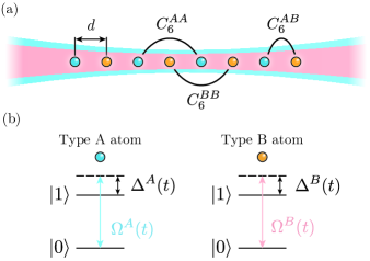
Figure 1: The two-species Rydberg atom array model. (a) Two-species neutral atom arrays are alternatively arranged into one-dimensional lattice with uniform spacing $d$ via optical tweezers where three kinds of interactions naturally emerge. (b) Illustration of energy levels, detuning and external fields of type A and B atoms.

III Ground state phase diagram

The phase diagram of one-species Rydberg atom array has been throughly studied. In the classical limit $\Omega=0$, the ground states form a series of Rydberg crystal states and these transitional symmetry breaking states can be characterized by two coprime integer $p$ and $q$, where $q$ denotes the size of the unit cell and $p$ the number of Rydberg-state atoms in each unit cell. When quantum fluctuation is taken into consideration, i.e., $\Omega\neq 0$, the phase diagram still exhibits transitional symmetry breaking crystalline ground states denoted $\mathbb{Z}_{2},\mathbb{Z}_{3},\cdots,\mathbb{Z}_{q}$ with excitation density $1/2,1/3,\cdots,1/q$, and other area of the phase diagram is mainly dominated by the disordered phase [12]. Besides the disordered and crystalline states, the so-called floating phase lives between disordered and crystalline phases which is predicted nummerically earlier and observed in experiment until recently [28, 12].

The phase diagram is more complicated when we consider two-species atom arrays. In one-species atom array, the interaction decays rapidly ($\sim 1/r^{6}$) and the phase diagram can be understood using the blockade mechenism. However, in two-species atom array, the interaction certainly will not decay monotonically and in some cases the interactions strength between nearest neighbour $C_{6}^{AB}/d^{6}$ and next nearest neighbour $C_{6}^{AA}/(2d)^{6},C_{6}^{BB}/(2d)^{6}$ atoms can be very close thus leading to competitions of different configurations which may give birth to novel ground states that cannot be observed in one-species Rydberg atom arrays. Theoretically, there has been some investigations about the Ising model with nearest and next nearest neighbour interactions, i.e., the axial next-nearest neighbor Ising (ANNNI) model whose Hamiltonian reads

$$\hat{H}_{\mathrm{ANNNI}} = -J_{1}\sum_{i}\hat{\sigma}^{z}_{i}\hat{\sigma}^{z}_{i+1}-J_{2}\sum_{i}\hat{\sigma}^{z}_{i}\hat{\sigma}^{z}_{i+2}$$ (4)

$$-B\sum_{i}\hat{\sigma}^{x}_{i},$$

We further denote $h=B/J_{1}$ and the frustration parameter $\kappa=-J_{2}/J_{1}$ [29]. When $\kappa>1/2$ and $h=0$, this model exhibits a so called anti-phase where the ground-state has a period of $4$ with two down-spins following two up-spins ($\ket{\uparrow\uparrow\downarrow\downarrow}$). If one turns on the transverse field ($h>0$), the floating phase can be found between the paramagnetic phase and the anti-phase [30, 29, 31]. However, the above theretical predictions have never been found to exist in any materials or any quantum simulation platforms.

Due to the Ising like interaction and the competition of nearest and next nearest neighbour interactions, we anticipate that the anti-phase can be found in the two-species Rydberg atom array, and indeed after extensive calculations of atoms’ real energy potentials we found there are some $C_{6}$ coefficients that can induce the anti-phase ground state predicted by the ANNNI model and several more verstile phases beyond the description of the ANNNI model.

III.1 Classical limit

Table 1: We list all the state configurations and their notations appeared in the main text and Appendix A for collation. The configurations listed here can be regarded under periodic boundary condition or in a infinite system size and we use $\ket{0}=\ket{\circ}$ and $\ket{1}=\ket{\bullet}$ to represent ground and excited state. The first atom of each following configuration is always A atom just like in Eq. (5) and (6). We also provide the unit cell length of the combined system $q$, the excitation number in each unit cell $p$ and the excitation density $n=p/q$ in the table.

Notation	Configuration	$q$	$p$	$n$
$\ket{\mathbb{D}}_{A}\ket{\mathbb{D}}_{B}$	$|\bullet\bullet\bullet\bullet\bullet\bullet\bullet\bullet\bullet\bullet\bullet\bullet\rangle$	2	2	1
$\ket{\mathbb{Z}_{2}}_{A}\ket{\mathbb{Z}_{2}}_{B}$	$|\bullet\bullet\circ\circ\bullet\bullet\circ\circ\bullet\bullet\circ\circ\rangle$	4	2	1/2
$\ket{\mathbb{Z}_{3}}_{A}\ket{\mathbb{Z}_{3}}_{B}$	$|\bullet\bullet\circ\circ\circ\circ\bullet\bullet\circ\circ\circ\circ\rangle$	6	2	1/3
$\ket{\mathbb{Z}_{4}}_{A}\ket{\mathbb{Z}_{4}}_{B}$	$|\bullet\bullet\circ\circ\circ\circ\circ\circ\bullet\bullet\circ\circ\circ\circ\circ\circ\rangle$	8	2	1/4
$\ket{\mathbb{Z}_{2}}_{A}\ket{\mathbb{D}}_{B}$	$|\bullet\bullet\circ\bullet\bullet\bullet\circ\bullet\bullet\bullet\circ\bullet\rangle$	4	3	3/4
$\ket{\mathbb{Z}_{3}}_{A}\ket{\mathbb{D}}_{B}$	$|\bullet\bullet\circ\bullet\circ\bullet\bullet\bullet\circ\bullet\circ\bullet\rangle$	6	4	2/3
$\ket{\mathbb{D}}_{A}\ket{\mathbb{Z}_{2}}_{B}$	$|\bullet\bullet\bullet\circ\bullet\bullet\bullet\circ\bullet\bullet\bullet\circ\rangle$	4	3	3/4
$\ket{\mathbb{D}}_{A}\ket{\mathbb{Z}_{3}}_{B}$	$|\bullet\bullet\bullet\circ\bullet\circ\bullet\bullet\bullet\circ\bullet\circ\rangle$	6	4	2/3
$\ket{\mathbb{Z}_{3}}_{A}\ket{\mathbb{Z}_{3}^{2}}_{B}$	$|\bullet\bullet\circ\circ\circ\bullet\bullet\bullet\circ\circ\circ\bullet\rangle$	6	3	1/2
$\ket{\mathbb{Z}_{3}^{2}}_{A}\ket{\mathbb{Z}_{3}}_{B}$	$|\bullet\bullet\bullet\circ\circ\circ\bullet\bullet\bullet\circ\circ\circ\rangle$	6	3	1/2
$\ket{\mathbb{Z}_{3}^{2}}_{A}\ket{\mathbb{D}}_{B}$	$|\bullet\bullet\bullet\bullet\circ\bullet\bullet\bullet\bullet\bullet\circ\bullet\rangle$	6	5	5/6
$\ket{\mathbb{D}}_{A}\ket{\mathbb{Z}_{3}^{2}}_{B}$	$|\bullet\bullet\bullet\bullet\bullet\circ\bullet\bullet\bullet\bullet\bullet\circ\rangle$	6	5	5/6
$\ket{\mathbb{Z}_{3}}_{A}\ket{\mathbb{Z}_{2}}_{B}$	$|\bullet\bullet\circ\circ\circ\bullet\bullet\circ\circ\bullet\circ\circ\rangle$	12	5	5/12

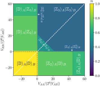
Figure 2: Classical phase diagram of Hamiltonian $\hat{H}_{1}$ in Eq. (3) with $V_{AB}\equiv C_{6}^{AB}/d^{6}=-1$ the energy unit and $V_{AA}\equiv C_{6}^{AA}/d^{6},V_{BB}\equiv C_{6}^{BB}/d^{6}$ here. The whole phase diagram is symmetric about the $V_{AA}=V_{BB}$ white dashed line. The excitation density $n$ serves as the order parameter to distinguish different phases here. Two grey dashed lines correspond to $V_{AA}=0$ and $V_{BB}=0$ respectively.

In the classical limit $\Omega=0$, only $\Delta$ and the interaction strengths $C_{6}^{AA}$, $C_{6}^{BB}$, $C_{6}^{AB}$ dominate the Rydberg atom array. In the $\ket{0},\ket{1}$ basis, all eigenstates of the system Hamiltonian are product states so we use $\ket{\mathbb{Z}_{p}^{q}}$ ($\ket{\mathbb{D}}$) to label different ordered (disordered) product states in each sublattice. For example, we use $\ket{\mathbb{Z}_{2}}_{A}\ket{\mathbb{Z}_{2}}_{B}$ and $\ket{\mathbb{Z}_{3}^{2}}_{A}\ket{\mathbb{Z}_{3}}_{B}$ to denote $\ket{11001100\cdots}$ and $\ket{111000111000\cdots}$ respectively. Their interpretation is shown below

$$\ket{\mathbb{Z}_{2}}_{A}\ket{\mathbb{Z}_{2}}_{B} = \ket{1010\cdots}_{A}\ket{1010\cdots}_{B}$$ (5)

$$= \ket{1}_{A}\ket{1}_{B}\ket{0}_{A}\ket{0}_{B}\cdots,$$

$$\ket{\mathbb{Z}_{3}^{2}}_{A}\ket{\mathbb{Z}_{3}}_{B} = \ket{110110\cdots}_{A}\ket{100100\cdots}_{B}$$ (6)

$$= \ket{1}_{A}\ket{1}_{B}\ket{1}_{A}\ket{0}_{B}\ket{0}_{A}\ket{0}_{B}\cdots,$$

where $\ket{\mathbb{Z}_{q}^{p}}$ stands for a state with unit cell length $q$ and excitation number $p$ and we use $\ket{\mathbb{Z}_{q}}=\ket{\mathbb{Z}_{q}^{1}}$ for simplicity. To find proper Rydberg states that exactly produce $\ket{\mathbb{Z}_{2}}_{A}\ket{\mathbb{Z}_{2}}_{B}=\ket{11001100\cdots}$ and $\ket{\mathbb{Z}_{3}^{2}}_{A}\ket{\mathbb{Z}_{3}}_{B}=\ket{111000111000\cdots}$ states, we calculate the classical phase diagram when $\Delta=0$ as shown in Fig. 2 where the meaning of all these phase labels can be found in Table 1. When the four parameters satisfy some particular conditions (see Fig. 2), we then obatin ground states with period-4 pattern such as $\ket{\mathbb{Z}_{2}}_{A}\ket{\mathbb{Z}_{2}}_{B}$ which is the abovementioned anti-phase and period-6 pattern such as $\ket{\mathbb{Z}_{3}^{2}}_{A}\ket{\mathbb{Z}_{3}}_{B}$. We have found some interaction strengths ($C_{6}$ coefficients) of real atoms, for example, Rb and Cs or ⁸⁵Rb and ⁸⁷Rb with corresponding $\Delta$ revealing period-4 and period-6 ground states. These data are shown in Table 2 which are selected from the interaction strength calculated from python package ARC [32]. A more systematic analysis on the classical phase diagram are provided in Appendix A.

Table 2: Hamiltonian parameters revealing period-4 $\ket{1100\cdots}$ and period-6 $\ket{111000\cdots}$ ground states. $(n_{1},n_{2})$ is the principal quantum number of two atoms. The unit of $C_{6}$ coefficients is $\mathrm{GHz}\cdot\mu\mathrm{m}^{6}$. All the coefficents are calculated from the dipole-dipole interactions between two species atoms. The first(second) row gives rise to the $\ket{1100\cdots}$($\ket{111000\cdots}$) ground states attached with the Rydberg state $\ket{88S_{1/2}}_{\mathrm{Rb}}\ket{86S_{1/2}}_{\mathrm{Cs}}$ ($\ket{52S_{1/2}}_{\mathrm{{}^{85}Rb}}\ket{80S_{1/2}}_{\mathrm{{}^{87}Rb}}$). All the interaction data are calculated via the python package ARC [32].

$(n_{1},n_{2})$	$C^{AA}_{6}$	$C^{BB}_{6}$	$C^{AB}_{6}$	$\Delta\cdot d^{6}/\mathrm{GHz\cdot\mu m^{6}}$
$(88,86)$	12696.34	7537.29	$-131.93$	$[-46.875,93.75]$
$(52,80)$	24.83	4161.55	$-2.16$	$[-1.23,0.04]$

III.2 Quantum Phase Diagram

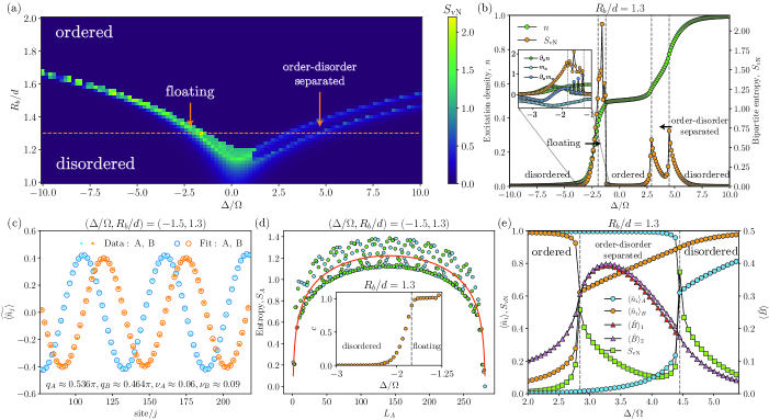
Figure 3: Phase diagram of Hamiltonian (1) with $C_{6}$ coefficients from the first line of Table 2. We choose the system size to be $N=282$ in the DMRG calculations. (a) Bipartite entanglement entropy $S_{\mathrm{vN}}$ unfolds four phases in the $(\Delta/\Omega,R_{b}/d)$-plane, including the disordered phase, the half filling ordered phase $\ket{1100\cdots}$, the order-disorder separated phase and the floating phase. (b) Excitation density $n$ and bipartite entanglement entropy $S_{\mathrm{vN}}$ along the orange dashed line $R_{b}/d=1.3$ are carefully calculated where the order-disorder separated phase area can be identified when $2.8\lesssim\Delta/\Omega\lesssim 4.5$. Inset: Besides $n$ and $S_{\mathrm{vN}}$, we also calculated the derivatives of $n$ and $m_{x}$ along the $x=\Delta/\Omega$ axis where $m_{x}\equiv\sum_{i}\langle\hat{\sigma}^{x}_{i}\rangle/N$. (c) The Friedel oscillation of local excitation density in the floating phase caused by OBC acting as an impurity is fitted using Eq.(8). The blue and orange dots represent data point of A and B atoms and the circles with corresponding color is the fitting result. To avoid edge effects, the fitting window is restricted to the range $j\in[76,219]$. (d) The bipartite entanglement entropy as a function of subsystem size $L_{A}$ is calculated to numerically extract the central charge where the green and blue dots stands for the entropy at $A|B$ and $B|A$ bond respectively. The orange curve is given by the fitting result and the extracted central charge is $c\approx 1.037$ for $(\Delta/\Omega,R_{b}/d)=(-1.5,1.3)$. Inset: the central charge extracted using the relation between entanglement entropy $S_{\mathrm{vN}}$ and correlation length $\xi$ (see Eq. 11 in the main text) varies with $\Delta/\Omega$ where $R_{b}/d=1.3$ is fixed from which the disordered phase and the floating phase can be easily distinguished. (e) The excitation density in both sublattices exhibits sudden change at different location with increasing $\Delta/\Omega$ thus causing a novel order-disorder separated phase where the translational symmetry only breaks among A atoms instead of B. The bond energy $\langle\hat{B}\rangle$ between neighbouring B atoms can serve as an order parameter to capture the boundary of this non-trivial phase. The slight difference between bond energy at different position $\langle\hat{B}\rangle_{1},\langle\hat{B}\rangle_{2}$ indicates a weak translational symmetry breaking in B atom sublattice caused by the complete translational symmetry breaking in A atom sublattice.

Now we mainly focus on the ground-state phase diagram of the system with the parameters shown in the first row of Table 2. There are two free tuning parameters, which are chosen as $\Delta/\Omega$ and $R_{b}/d$ ($R_{b}\equiv\sqrt[6]{|C_{AB}|/\Omega}$) and $\Omega=1$ is fixed in the following numerical calculations. We use exact diagonalization (ED) and density matrix renormalization group (DMRG) [33, 34, 35] methods to calculate the ground state of the system. We perform ED simulations on $N=16$ systems with periodic boundary conditions (PBC) and DMRG calculations on system size $N=282$ with open boundary conditions (OBC), where $N=4n+2$ ($n\in\mathbb{N}^{+}$) can fit the particle distributions under OBC. In DMRG calculations, we consider the long-range interactions up to eight atom spacings. We keep the bond dimensions up to $512$, which can give very accurate results with the truncation error about $10^{-10}$.

To map out the phase diagram, we first calculate the bipartite entanglement entropy $S_{\mathrm{vN}}=-\mathrm{Tr}\rho_{A}\ln\rho_{A}$, where $\rho_{A}$ is the reduced density matrix of the subsystem in the middle. The results are shown in Fig. 3(a). Similar to the one-species system, the state in the small $R_{b}$ regime mainly depends on $\Delta/\Omega$. While the empty state $\ket{0000\cdots}$ and polarized state $\ket{1111\cdots}$ are favored at a large negative and positive $\Delta/\Omega$, respectively, a paramagnetic state is realized near $\Delta/\Omega=0$ (not shown here). In this paper, we denote all these states as disordered states in terms of no transitional symmetry breaking. With growing interactions, the ordered $\ket{1100\cdots}$ state breaking translational symmetry dominates the phase diagram. Besides, we identify a floating phase and an order-disorder separated phase with enhanced entanglement entropy.

To explicitly demonstrate the quantum phases, we scan along the parameter line with fixed $R_{b}/d=1.3$, as shown in Fig. 3(b), which characterizes the phases by excitation density $n$ and entropy. We first discuss the floating phase, which can be well described by the Luttinger-liquid theory, and the power-law decay of correlation functions is controlled by the Luttinger parameter $K$. Due to the gapless nature, the floating phase can hardly be identified in a small system size, thus we carefully examine the DMRG results. The open boundary in DMRG calculations acts as an impurity that can lead to the Friedel oscillation of excitation density (also the bipartite entropy, see Fig. 3(d)). According to Boundary Conformal Field Theory (BCFT), the density profile generally can follow the behavior [29, 36, 37]

$$\langle\hat{n}_{j}\rangle = \overline{\langle\hat{n}_{j}\rangle}+(-1)^{\lfloor j/2\rfloor}\widetilde{\langle\hat{n}_{j}\rangle},$$ (7)

$$\widetilde{\langle\hat{n}_{j}\rangle} \propto \frac{\cos(qj+\alpha)}{[(N/\pi)\sin(\pi j/N)]^{K}},$$ (8)

where $K$ is the Luttinger parameter, $q$ is the wave-vector that can be incommensurate, and $\alpha$ is the phase shift. However, the unit cell of our system is composed of two different atoms. Therefore, in principle we should regard this system as two different bosonic fields coupling with each other, which characterize the low-energy bosonic excitations in the sublattice A and B, respectively, with different Luttinger parameters $K_{A},K_{B}$. Due to the interaction between the two sublattices, the Luttinger parameters should be mixed so the results by fitting Eq. (8) in each sublattice are not the exact Luttinger parameters, which we denote as $\nu_{A},\nu_{B}$ instead of $K_{A},K_{B}$. The relation between $\nu_{A},\nu_{B}$ and $K_{A},K_{B}$, also including the coupling parameter, can be derived from the two component bosonic field Hamiltonian which is written as

$$H = \displaystyle\frac{v_{A}}{2}\int\mathrm{d}x\left[K_{A}\Pi_{A}^{2}+\frac{1}{K_{A}}\left(\frac{\mathrm{d}\phi_{A}}{\mathrm{d}x}\right)^{2}\right]$$ (9)

$$+ \displaystyle\frac{v_{B}}{2}\int\mathrm{d}x\left[K_{B}\Pi_{B}^{2}+\frac{1}{K_{B}}\left(\frac{\mathrm{d}\phi_{B}}{\mathrm{d}x}\right)^{2}\right]$$

$$+ \ \text{coupling terms},$$

where $\Pi_{i}$ is the momentum density variable canonically conjugate to $\phi_{i}$, and $v_{i}$ is the velocity of the corresponding gapless low-energy excitations [37, 38]. We extract the parameters $\nu_{A},\nu_{B}$ and incommensurate wavevectors $q_{A},q_{B}$ at $(\Delta/\Omega,R_{b}/d)=(-1.5,1.3)$, by fitting the Friedel oscillation of the two sublattices separately, giving the results $q_{A}\approx 0.536\pi$, $q_{b}\approx 0.464\pi$, and $\nu_{A}\approx 0.06$, $\nu_{B}\approx 0.09$, as shown in Fig. 3(c).

We further characterize the gapless nature of the floating phase through central charge. We first use the formula of entanglement entropy at a critical point in a finite-size chain with OBC to extract the central charge. According to the CFT, the relation between the entanglement entropy of a subsystem $S_{A}$ and the subsystem size $L_{A}$ is given as [39, 40, 41, 42, 43, 44]

$$S_{A}\sim\frac{c}{6}\log_{2}\left[\frac{2N}{\pi}\sin\left(\frac{\pi L_{A}}{N}\right)\right]+\log_{2}g+\frac{s_{1}}{2},$$ (10)

where $N$ is the system size and $g,s_{1}$ are non-universal constants. The DMRG results are shown in Fig. 3(d) and the extracted central charge is $c\approx 1.037$, which can be interpreted by approximately regarding the two-species Rydberg atom array as two interacting Ising chains [29, 45]. We also confirm the central charge by extracting the result from the VUMPS simulation using the following relation [46]

$$S_{\mathrm{vN}}=\frac{c}{6}\log_{2}\xi=\frac{c\kappa}{6}\log_{2}\chi,$$ (11)

where $S_{\mathrm{vN}}$ is the entropy, and $\xi$ is the correlation length that scales with the bond dimension $\chi$ as $\xi\propto\chi^{\kappa}$. We calculate the correlation lengths and entropies at different bond dimensions, which then are fitted to obtain the central charge. The results are shown in the inset of Fig. 3(d). The area where $c\approx 1$ is consistent with the floating phase region.

With further increased $\Delta/\Omega$, we identify another new phase between the $|1100\cdots\rangle$ and polarized phases. In this phase, the excitation density $\langle\hat{n}_{i}\rangle$ of the A atoms breaks translational symmetry but that of the B atoms is uniform, as demonstrated in Fig. 3(e). Since the A sublattice persists the density-wave-like state, the increased excitation density mainly concentrates in the B atoms. For this reason, we dub this phase as an order-disorder separated phase.

In such a state, the mirror symmetry with respect to a B atom is simultaneously broken, which can be also characterized by the bond energy of neighboring B atoms. Interestingly, we find that the dominant bond energy term $\langle\hat{n}_{i}\hat{n}_{i+2}\rangle$ are still invariant for B atoms, but the transverse component $\langle\hat{B}\rangle\equiv\langle\hat{\sigma}^{+}_{i}\hat{\sigma}^{-}_{i+2}+h.c.\rangle$ can show a weak oscillation. As shown in Fig. 3(e) of the VUMPS [47] results in the thermodynamic limit, $\langle\hat{B}\rangle$ of the two neighboring B atoms with an excited A atom in the middle ($\langle\hat{B}\rangle_{1}$) is slightly lower than that with an A atom possessing very small density ($\langle\hat{B}\rangle_{2}$), characterizing the broken mirror symmetry with respect to the B atom.

We also study the phase diagram using mean-field method and the mean-field result is able to capture almost all phases but fails to predict the floating phase. Phase diagram of the Hamiltonian (1) with the $C_{6}$ coefficients from the second line of Table 2 is also calculated which is very similar to the period-4 case. The main difference is the more obvious order-disorder separated (more precisely, half ordered) phase area between ordered and disordered phase. See Appendix C for more information.

IV Quench Dynamincs

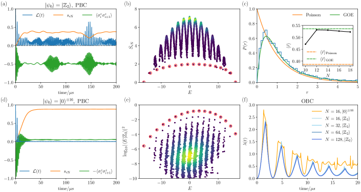
Figure 4: Evidence of the existence of quanutm many-body scars in the two-species Rydberg atoms array. Here we fix atom number $N=16$, atom spacing $d=9$ and use the data from the first line of Table 2. The external field strength is chosen to be $(\Omega,\Delta)=(2,0.05)$. (a) Quanutm quench from initial state $\ket{\mathbb{Z}_{2}}$ shows non-thermalizing behaviour of the system where we calculated the Loschmidt echo $\mathcal{L}(t)=|\langle\psi_{0}|e^{-i\hat{H}t}|\psi_{0}\rangle|^{2}$, the bipatite entanglement entropy per atom of the half system $s_{\mathrm{vN}}$ and the average correlation function $\langle\sigma^{z}_{i}\sigma^{z}_{i+1}\rangle=\sum_{i}\langle\hat{\sigma}^{z}_{i}\hat{\sigma}^{z}_{i+1}\rangle/N$. (b) Bipartite entanglement entropy of all the eigenstates is depicted in the eigenenergy-entropy plane where those approximate quantum many-body scar states are marked with red circles. (c) Level spacing distribution of the system in the symmetry reduced sector (momentum $k=0$, inversion even sector) fits well with the distribution given by Gaussian Orthogonal Ensemble (GOE) instead of Poisson distribution indicating this system is very likely to be chaotic. Inset: Level spacing indicator $\langle\tilde{r}_{i}\rangle$ as a function of system size $N$. Orange(Green) dashed line is given by Poisson(GOE) distribution. (d) Quanutm quench from initial empty state $\ket{0}^{\otimes 16}$ shows fast thermalization compared with $\ket{\mathbb{Z}_{2}}$. (e) Overlaps between $\ket{\mathbb{Z}_{2}}$ and scar states are marked with red circles and they contribute more significantly to the system dynamics than other eigenstates(unmarked dots). (f) The Loschmidt rate $\lambda(t)=-\frac{1}{N}\ln\mathcal{L}(t)$ exhibits non-analytical behavior for initial $\ket{\mathbb{Z}_{2}}$ state indicating there might be a possible dynamical quantum phase transition.

It’s believed that the time evolution of complex quantum systems is dominated by the eigenstats thermalization hypothesis (ETH), i.e., systems which are initially prepared in far-from-equilibrium states can evolve in time to a state which appears to be in thermal equilibrium and such systems are called quantum ergodic [48, 49, 50]. However, not all quantum systems obey ETH. The simplest example is the one dimensional transverse field Ising model (TFIM) with only nearest neighbor interaction. The 1D TFIM can be exactly solved using Jordan-Wigner transformation indicating the quasiparticles are free so the system will not thermalize. Another example is the system revealing many-body localization where the disorder is so strong that there is countless quasi-local integrals of motion (LIOM) who help the system break ergodicity [51]. In these two examples, the symmetry or the conservation law plays an important role against ETH thus leading to strong ergodicity breaking [52].

Recent progress in experiments has made neutral atom system a very convincing platform for quantum simulation. Surprisingly, it has been observed that the one dimensional Rydberg atom arrays exhibit non-thermalizing phenomenon for some certain initial states such as $\ket{\mathbb{Z}_{2}}=\ket{1010\cdots}$, i.e., the Loschmidt echo shows revivals over time [12]. There has been plenty of theoretical study of this phenomenon and it’s found that in the spectrum of the low energy effective Hamiltonian of the Rydberg atom arrays (the “PXP” Hamiltonian), there exists some slightly entangled eigenstates who have much larger overlap with initial state $\ket{\mathbb{Z}_{2}}$ than other eigenstates [24, 25, 26, 27]. These eigenstates are called quantum many-body scars (QMBS) and they cause the weak ergodicity breaking in the Rydberg atom system.

In the two-species Rydberg atom arrays, we find similar phenomenon in the time evolution and the approximate QMBS in the system spectrum can be well understood in the mean-field framework which is different from the one-species case.

The quench dynamics of our system also exhibits revivals in Loschmidt echo $\mathcal{L}(t)$ over time with the initial state $\ket{\psi_{0}}$ a Néel state $\ket{\mathbb{Z}_{2}}=\ket{1010\cdots}$ (Fig. 4(a)). The Loschmidt echo is defined by $\mathcal{L}(t)=|\langle\psi_{0}|e^{-i\hat{H}t}|\psi_{0}\rangle|^{2}$ with $\hat{H}$ the system Hamiltonian (1). Our system does not reveal integrability due to the fact that the distribution of the ratio of consecutive level spacing $P(r)$ fits well with the one given by the random matrix theory ensembles instead of Poisson distribution which can be found in many integrable models as shown in Fig. 4(c) [53]. Therefore, the revival of Loschmidt echo is a non-trivial phenomenon because the system now will not thermalize with certain initial states. We numerically diagonalize the system Hamiltonian and find there are some eigenstates who has much lower bipartite entropy than other eigenstates (Fig. 4(b)) and their overlap with initial state $\ket{\mathbb{Z}_{2}}$ are anomalously enhanced (Fig. 4(e)). The low entropy eigenstates are in fact approximate quantum many-body scars and they can be approximately built by the quasi-particle operators in the mean-field framework.

To analytically explain these phenomenon, we first map the Rydberg system Hamiltonian to a simpler Hamiltonian, the quantum ANNNI model Hamiltonian. This is reasonable because the long-range interactions will not contribute much to the system dynamics and two $C_{6}$ coefficents $C^{AA}_{6},C^{BB}_{6}$ are so close that we can ignore their difference here. The quantum ANNNI model Hamiltonian is similar to a Kitaev chain after performing Jordan-Wigner transformation and the mean-field approximation, where the only difference is the next nearest fermion hopping terms and the Cooper pair creation(annihilation) operator terms. The effective Hamiltonian reads

$$\hat{H} = \frac{\tilde{\Omega}}{2}\sum_{n}(2\hat{c}_{n}^{\dagger}\hat{c}_{n}-1)+V_{1}\sum_{n}(\hat{c}_{n}-\hat{c}_{n}^{\dagger})(\hat{c}_{n+1}^{\dagger}+\hat{c}_{n+1})$$ (12)

$$+\tilde{V}_{2}\sum_{n}(\hat{c}_{n}-\hat{c}_{n}^{\dagger})(\hat{c}_{n+2}^{\dagger}+\hat{c}_{n+2}),$$

where $\hat{c}_{n}$ is the spinless fermion operator, and $\tilde{\Omega},V_{1},\tilde{V}_{2}$ controls the chemical potential, nearest and next neatest hopping as well as pair creation and annihilation terms respectively.

We claim that the low bipartite entanglement entropy eigenstates (denoted $\ket{s_{n}},n=0,1,\cdots,N$) mainly fall into the subspace composed of zero momentum Cooper pairs ($\hat{\beta}^{\dagger}_{k}\hat{\beta}^{\dagger}_{-k}$) and single fermion ($\hat{c}_{k=0}^{\dagger}$), i.e., they can be well constructed using the states $\ket{\psi_{\{n_{k}\}}^{\mathrm{ABC}}}$ for even $n$ or $\ket{\psi_{\{n_{k}\}}^{\mathrm{PBC}}}$ for odd $n$ in Eq. (13),

$$\ket{\psi_{\{n_{k}\}}^{\mathrm{ABC}/\mathrm{PBC}}} = \prod_{k}^{\mathcal{K}_{+}^{\mathrm{ABC}/\mathrm{PBC}}}(\hat{\beta}_{k}^{\dagger}\hat{\beta}_{-k}^{\dagger})^{n_{k}}\ket{\emptyset}^{\mathrm{ABC}/\mathrm{PBC}},$$ (13)

where $\mathcal{K}_{+}^{\mathrm{ABC}}=\left\{k=(2m-1)\pi/N,m=1,\cdots,N/2\right\}$, $\mathcal{K}_{+}^{\mathrm{PBC}}=\left\{k=2m\pi/N,m=1,\cdots,N/2-1\right\}$, $\hat{\beta}_{k}^{\dagger}\hat{\beta}_{-k}^{\dagger}$ is the excitation operator of Cooper pair with momentum $(k,-k)$, $n_{k}=0,1$ is the number of Cooper pair excitation at $(k,-k)$, $\ket{\emptyset}^{\mathrm{ABC}}$ is the ground state of the system in anti-periodic boundary condition(ABC) sector and $\ket{\emptyset}^{\mathrm{PBC}}$ is the ground state in PBC sector. The overlap between the states constructed by quasipaticle operators and the exact low entanglement entropy eigenstates obtained via ED in the ANNNI model of small size ($N=16$) is at least 0.89, which explains these approximate quantum many-body scars to a great extent, i.e., the system basically only evolves in the zero momentum symmetry sector if the initial state is $\ket{\mathbb{Z}_{2}}$. We refer interested readers to Appendix F for more detailed calculation and discussion.

With the system’s size getting larger, the revival of Loschmidt echo $g(t)$ becomes inconspicuous. However, we can define the Loschmidt rate for finite size system [54]

$$\lambda(t)=-\frac{1}{N}\ln\mathcal{L}(t),$$ (14)

and we observe there are discontinous points of $\lambda(t)$ in time as shown in Fig. 4(f) indicating the dynamical quantum phase transition(DQPT) might happen at these time points which can be explained by mainly considering the contribution of the approximate QMBS to the system dynamics. We refer interested readers to Appendix G for more discussions.

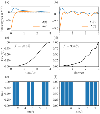
Figure 5: The optimization results of $\ket{1100\cdots}$ and $\ket{111000\cdots}$ preparation in small system ($N=10$ for $\ket{1100\cdots}$ and $N=9$ for $\ket{111000\cdots}$) are shown in the left and right column respectively. The first line shows the required pulse of $\Omega(t)$ as well as $\Delta(t)$ and the second line shows the fidelity $\mathcal{F}(t)$ over time and the local excitation density $\langle\hat{n}_{i}\rangle$ of the prepared state is depicted in the last row. The total evolution time $T$ for both states is $T=3\ \mu s$ and we choose $d=5\ \mu m$ for $\ket{1100\cdots}$ state preparation and $d=3\ \mu m$ for $\ket{111000\cdots}$ preparation.

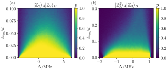
Figure 6: Numerical simulations of the robustness of $\ket{1100\cdots}$(a) and $\ket{111000\cdots}$(b) ordered states where at each point $(\Delta,\delta d_{m}/d)$ the real distances between neighbouring atoms $\{d_{n}\}$ are randomly generated for 2000 times with $|d_{n}-d|<\delta d_{m},\forall n$ satisfied and the situations that the system still holds ordered ground states are counted to further calculate the survival probability $p\in[0,1]$ of the ordered ground states depicted above.

V Ground State Preparation and Robustness

Next we try to prepare the ground states in the ordered phase of the two-species Rydberg atom array. To be specific, we begin from product state $\ket{0000\cdots}$ where there is barely no interaction between atoms and turn on the laser to let the system evolve to the ordered state such as $\ket{1100\cdots}$ via some controlled time dependent external fields. We define the fidelity function as

$$\mathcal{F}[\Omega(t),\Delta(t)]=|\langle\psi_{t}|\hat{U}|\psi_{0}\rangle|^{2},$$ (15)

$$\hat{U}=\mathcal{T}\exp\left(-i\int_{0}^{T}\mathrm{d}t\ \hat{H}[\Omega(t),\Delta(t)]\right),$$ (16)

where $\hat{H}(t)$ is the system Hamiltonian (1), $\mathcal{T}$ is the time ordering operator, $T$ is the total evolution time and $\ket{\psi_{0}}$($\ket{\psi_{t}}$) is the initial(target) state. Fidelity, which we aim to maximize, is a functional depending on $\Omega(t)$ and $\Delta(t)$. In order to find the control pulse $\Omega(t)$ and $\Delta(t)$ for the time evolution required, we use dressed Chopped RAndom Basis(dCRAB) method [55, 56]. For states in the ordered phase such as $\ket{1100\cdots}$ and $\ket{111000\cdots}$, using dCRAB method, we found some pulses for $\Omega(t)$ and $\Delta(t)$ such that the required states can be obtained after time evolution. These pulses are shown in Fig. 5.

The robustness of these novel ordered ground states is vital to their experimental preparation. We thus study the robustness of these states where we mainly consider the imperfection of interatomic spacings. In experiments, the atom will deviate from equilibrium position due to thermal fluctuations and the influence from environment leading to the slight change in interaction strength. The robustness of the period-4 and period-6 ordered states are shown in Fig. 6 where the vertical axis $\delta d_{x}/d,\delta d_{y}/d$ represents the maximum distance of deviation from the central position in $x$ and $y$ directions. The numerical results indicates that both $\ket{1100\cdots}$ and $\ket{111000\cdots}$ states are robust when only the deviation from the central position is considered.

VI Discussion and Outlook

We study the phase diagram of the two-species Rydberg atom array and find the complex interactions induced by the atom species can give birth to many novel state configurations which cannot be observed in a single-species atom array such as the period-4 and period-6 product states. We note that using adiabatic evolution assisted by optimal control methods one can prepare these novel ordered states in experiements and we have already verified that these ordered states are stable against part of the environment noise. Therefore we believe we can experimentally prepare and observe these novel ordered states in near future. The interplay between quantum fluctuations and atomic interactions leads to other novel phases including the order-disorder separated phase and the floating phase. The order-disorder separated phase has never been reported in cold atom system or other quantum simulation platforms. The floating phase in single-species atom array has been fully studied and recently has been experimentally observed in a ladder atom array. However, we remark that unlike in single-species case where the floating phase is described by a free bosonic field theory, in two-species atom array, one need two interacting bosonic fields to describe the floating phase thus there are more theoretical insights in the two-species case.

The two-species Rydberg atom array can also exhibit quantum many-body scars in the energy spectrum similar to the “PXP” model and their large overlap with initial $\ket{\mathbb{Z}_{2}}$=$\ket{1010\cdots}$ state can also induce revivals in Loschmidt echo over time. We approximately map two-species atom array Hamiltonian to the quantum ANNNI model Hamiltonian and found that the time evolution of $\ket{\mathbb{Z}_{2}}$ is mainly restricted in the momentum-zero subspace and the scarred eigenstates can be well constructed using the quasi-particle operators of Cooper pair form with zero momentum. We stress that unlike “PXP” model the ergodicity breaking phenomenon is induced by the proper perturbations instead of the Rydberg blockade mechenism. Furthermore, it should also be emphasized that the DQPT found in the same system can be explained by the newly discovered scarred states which is the first time the connection between QMBS and DQPT is established.

Our current work lays the foundation for quantum simulation using two-species Rydberg atom array. The various novel classical ground state configurations are ideal platform for simulating abundant charge density wave states in condensed matter system and our results considering quantum fluctuations have also paved the way for studying quanutm phase transitions and other critical phenomenon in the two-species Rydberg atom array. Our study of quench dynamics also shows that the two-species Rydberg atom array can be utilized to explore the mechenism of ergodicity breaking as well as its relation with DQPT and etc. In conclusion, the two-species Rydberg atom array provide a new platform for us to explore more complex quantum phenomenon and our work suggest this platform can be realized in experiements convincingly.

Appendix A Discussion on the classical phase diagram

We consider the classical situation where there is no transverse field $\Omega=0$. In order to simplify our discussion, we also set $\Delta=0$, i.e., we only study the phase diagram of the Hamiltonian $\hat{H}_{1}$ in Eq. (3). We define $V_{AA}=C_{6}^{AA}/d^{6},V_{BB}=C_{6}^{BB}/d^{6},V_{AB}=C_{6}^{AB}/d^{6}$ and choose $V_{AB}$ as the energy unit. We set $V_{AB}=-1$ to introduce competition of different states. The classical phase diagram has already been shown in Fig. 2, where we use excitation density $n\equiv\frac{1}{N}\sum_{i}\langle\hat{n}_{i}\rangle$ as the order parameter to distinguish different phases ($N$ is the system size). In Fig. 2, the system size can be considered as towards infinity $N\to\infty$.

The classical phase diagram is symmetric about the line $V_{AA}=V_{BB}$ marked with a white dashed line in Fig. 2. We discuss a simpler case with $V_{AA}=V_{BB}=V$. Since $V_{AB}=-1<0$, the system will prefer the neighboring excitation, and the positive next-nearest-neighbour interaction $V>0$ will lead to the crystalline ground states in each sublattice. Therefore, when $V$ is small the system prefers a disordered phase in the sublattices of both A and B atoms denoted as $\ket{\mathbb{D}}_{A}\ket{\mathbb{D}}_{B}$, and with growing $V$, the blockade mechenism begins to take effect, giving birth to different crystalline ground states with different excitation density including the abovementioned $\ket{11001100\cdots}$ configuration denoted as $\ket{\mathbb{Z}_{2}}_{A}\ket{\mathbb{Z}_{2}}_{B}$. The phase diagram along the $V_{AA}=V_{BB}$ line is summarized in Fig. 7. When $V_{AA}>0$ and $V_{BB}<0$ (or $V_{AA}<0$ and $V_{BB}>0$), the sublattice of atom A still tends to stay in crystalline states but the B atoms prefer a disordered state, which leads to the formation of a “half-ordered” phase denoted as $\ket{\mathbb{Z}_{q}}_{A}\ket{\mathbb{D}}_{B}$ (and $\ket{\mathbb{D}}_{A}\ket{\mathbb{Z}_{q}}_{B}$, $q=2,3,\cdots$).

Numerical simulations uncover two new phases beyond our simple analysis. We denote the first new phase as $\ket{\mathbb{Z}_{3}}_{A}\ket{\mathbb{Z}_{3}^{2}}_{B}$ (and also $\ket{\mathbb{Z}_{3}^{2}}_{A}\ket{\mathbb{Z}_{3}}_{B}$ because of symmetry), where $\ket{\mathbb{Z}_{q}^{p}}$ stands for a state with unit cell length $q$ and excitation number $p$. We use $\ket{\mathbb{Z}_{q}}=\ket{\mathbb{Z}_{q}^{1}}$ for simplicity. The $\ket{\mathbb{Z}_{3}}_{A}\ket{\mathbb{Z}_{3}^{2}}_{B}$ phase is found at the $V_{AA}\gg V_{BB}>0$ area, where the interaction strength between A atoms $V_{AA}$ is large enough to maintain a crystalline state $\ket{\mathbb{Z}_{3}}$ while $V_{BB}$ is too weak to do so, thus the influence of $V_{AB}$ persuades the system to realize a novel $\ket{111000111000\cdots}$ configuration (the first site is B atom here). Notice that because of the same excitation density of $\ket{\mathbb{Z}_{2}}_{A}\ket{\mathbb{Z}_{2}}_{B}$ and $\ket{\mathbb{Z}_{3}}_{A}\ket{\mathbb{Z}_{3}^{2}}_{B}$, these two phases share the same color in Fig. 2. While the $\ket{\mathbb{Z}_{3}}_{A}\ket{\mathbb{Z}_{3}^{2}}_{B}$ state mainly lives around $V_{AA}=0$ and $V_{BB}=0$ lines marked with grey dashed lines, the $\ket{\mathbb{Z}_{2}}_{A}\ket{\mathbb{Z}_{2}}_{B}$ state mainly dominates the area around the white dashed line not including the area close to grey dashed line. The second new phase is denoted as $\ket{\mathbb{Z}_{3}^{2}}_{A}\ket{\mathbb{D}}_{B}$ (and $\ket{\mathbb{D}}_{A}\ket{\mathbb{Z}_{3}^{2}}_{B}$), and it is located at the boundary between $\ket{\mathbb{D}}_{A}\ket{\mathbb{D}}_{B}$ and $\ket{\mathbb{Z}_{2}}_{A}\ket{\mathbb{D}}_{B}$ (also $\ket{\mathbb{D}}_{A}\ket{\mathbb{Z}_{2}}_{B}$). Due to the very small area, we do not label this phase in Fig. 2.

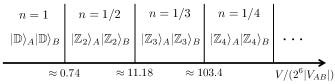
Figure 7: Phase diagram of Hamiltonian $\hat{H}_{1}$ in Eq. (3) along the white dashed line $V_{AA}=V_{BB}=V$ in Fig. 2 with $V_{AB}=C_{6}^{AB}/d^{6}=-1$ the energy unit.

We do not consider the influence of detuning $\Delta$, but it is worth being pointed out that the interplay between $\Delta$ and $V_{AA},V_{BB},V_{AB}$ will give birth to more complex configurations. For example, we find that when $V_{AA}=50\times 2^{6},V_{BB}=10\times 2^{6},V_{AB}=-1$ and $\Delta=1$, the ground state appears to be $\ket{\mathbb{Z}_{3}}_{A}\ket{\mathbb{Z}_{2}}_{B}$ with the excitation density $n=5/12$, which is not found in our analyses at $\Delta=0$. We leave the work of completing the classical phase diagram to future study, and the current results already suffice to instruct us to find the proper Rydberg states that can produce novel ground state configurations such as the anti-phase $\ket{1100\cdots}$ and etc.

Appendix B Interaction data for experimental setup

Our next step is to check whether it is possible to prepare these states in experiment. We calculate all the $C_{6}$ coefficents between the Rydberg states $\ket{n_{1}S_{1/2}}_{{}^{85}\mathrm{Rb}}$ and $\ket{n_{2}S_{1/2}}_{{}^{87}\mathrm{Rb}}$, as well as between $\ket{n_{1}S_{1/2}}_{\mathrm{Rb}}$ and $\ket{n_{2}S_{1/2}}_{\mathrm{Cs}}$, using the python package ARC [32], where $n_{1},n_{2}$ stand for the principal quantum number of the first and second atoms ranging from 40 to 90 with $m_{j}=1/2$ for all the states. We present the data points giving $C^{AB}_{6}<0$ on the phase diagram. The results for ${}^{85}\mathrm{Rb}$ and ${}^{87}\mathrm{Rb}$ atoms are shown in Fig. 8, and the results for $\mathrm{Rb}$ and $\mathrm{Cs}$ atoms are shown in Fig. 9. Notice that we only show the data points that satisfy $V_{AA}/(2^{6}|V_{AB}|)<100$, and we note that there are many data points are beyond this area but our figures are able to cover all the situations.

It can be concluded that for the atoms of the same element (for Rubidium atoms at least), it is almost impossible to prepare a $\ket{\mathbb{Z}_{2}}_{A}\ket{\mathbb{Z}_{2}}_{B}$ state only using the $S$ states. Because if the interaction between two $\mathrm{Rb}$ atoms at the $S$ state is strong ($V_{AA},V_{BB}>0$ are very large), the interaction $V_{AB}$ will be positive, leading to the empty ground state $\ket{0000\cdots}$ instead of $\ket{1100\cdots}$ state. To ensure $V_{AB}<0$ is always maintained, the two principal quantum numbers have to satisfy $|n_{1}-n_{2}|\gg 0$, and thus there will always be a small $V_{BB}$ and a large $V_{AA}$, which can only gives birth to other ground state configurations as shown in Fig. 8.

For $\mathrm{Rb}$ and $\mathrm{Cs}$ atoms, the above analysis also applies but numerical simulation finds some $C_{6}$ coefficents that can produce the $\ket{\mathbb{Z}_{2}}_{A}\ket{\mathbb{Z}_{2}}_{B}$ ground state, which indicates it is possible to prepare this anti-phase in experiment.

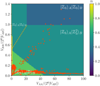
Figure 8: The real atom interaction $C_{6}$ coefficents are depecited above where ${}^{85}\mathrm{Rb}$ are denoted A atom and ${}^{87}\mathrm{Rb}$ B atom here. The orange dashed line is the boundary that distinguishes two different phases that have the same excitation density. We let $V_{AA}=C_{6}^{AA}$, $V_{BB}=C_{6}^{BB}$ and $V_{AB}=C_{6}^{AB}$ for simplicity and calculate the data points here.

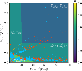
Figure 9: The real atom interaction $C_{6}$ coefficents are depecited above where $\mathrm{Rb}$ are denoted A atom and $\mathrm{Cs}$ B atom for blue points and for red points A(B) atom stands for $\mathrm{Cs}$($\mathrm{Rb}$). The orange dashed line is the boundary distinguishing two different phases that have the same excitation density. We let $V_{AA}=C_{6}^{AA}$, $V_{BB}=C_{6}^{BB}$ and $V_{AB}=C_{6}^{AB}$ for simplicity and calculate the data points here.

Appendix C Quantum phase diagram of the second parameter setup

In this section, we discuss the phase diagram of the Hamiltonian defined by the parameters in the second line of Table 2, which can realize the period-6 ground state. The DMRG results of the excitation density $n$ and entanglement entropy are demonstrated in Fig. 10. In the orange region of Fig. 10(a), the much larger $C_{6}$ coefficient between type B atoms leads to the formation of $\ket{\mathbb{Z}_{2}}$ Rydberg crystal in the sublattice of type B atoms. And the type A atoms form a full filling disordered state $\ket{1111\cdots}$, giving the total filling factor $3/4$. Thus, we denote this phase as the half-ordered phase because only half of the system is ordered (B sublattice).

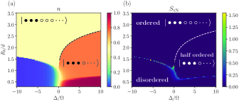
Figure 10: DMRG phase diagram of the Hamiltonian (1) with the $C_{6}$ coefficients from the second line of Table 2. We choose the system size to be $N=303$. (a) Different phases can be clearly identified by the excitation density $n$. (b) Boundaries between different phases are captured by the bipartite entanglement entropy $S_{\mathrm{vN}}$ except for the first order transition line which we mark with the white dashed line.

Appendix D Ground-state phase diagram based on the mean-field theory

In this section, we discuss the mean-field calculate of the phase diagram. Given the DMRG results, it is natural to choose the unit cell of four lattice spacings in the mean-field framework, i.e., four variational parameters in the following analysis, which is denoted as $\vec{n}=(n_{0},n_{1},\cdots,n_{L-1})$.

Following the mean-field approximation ($\delta\neq 0$)

$$\hat{n}_{i}\hat{n}_{i+\delta}\approx\langle\hat{n}_{i}\rangle\hat{n}_{i+\delta}+\hat{n}_{i}\langle\hat{n}_{i+\delta}\rangle-\langle\hat{n}_{i}\rangle\langle\hat{n}_{i+\delta}\rangle,$$ (17)

one can obtain the mean-field Hamiltonian for a unit cell

$$\hat{H}_{\mathrm{MF}}=\hat{H}_{0}+\hat{H}_{1}$$ (18)

with the part inside unit cell of length $L$

$$\hat{H}_{0}=\frac{\Omega}{2}\sum_{i=0}^{L-1}\hat{\sigma}_{i}^{x}-\Delta\sum_{i=0}^{L-1}\hat{n}_{i}+\sum_{i=0}^{L-2}\sum_{j=i+1}^{L-1}\frac{C_{6}^{ij}}{d^{6}|i-j|^{6}}\hat{n}_{i}\hat{n}_{j},$$ (19)

and the part derived from mean-field approximation

$$\hat{H}_{1} = \sum_{i=0}^{L-1}\sum_{j=0}^{L-1}\frac{C_{6}^{ij}}{d^{6}}c_{ij}n_{j}\hat{n}_{i}$$ (20)

$$c_{ij} = \sum_{n=0}^{+\infty}\left(\frac{1}{(6n+L+i-j)^{6}}+\frac{1}{(6n+L-i+j)^{6}}\right)$$

$$= \frac{1}{120L^{6}}\left[\psi^{(5)}\left(1+\frac{i-j}{L}\right)+\psi^{(5)}\left(1-\frac{i-j}{L}\right)\right]$$

where $C_{6}^{ij}$ is the $C_{6}$ coefficient between atom $i$ and $j$, $d$ is the atom spacing and $\psi^{(5)}(x)$ is the polygamma function of order 5.

For $L=4$, we numerically calculate the optimal choice of variational parameters $\vec{n}$ for the mean-field Hamiltonian $\hat{H}_{\mathrm{MF}}$. We denote the ground state of $\hat{H}_{\mathrm{MF}}$ as $\ket{\psi_{g}(\vec{n})}$ and define the energy density $\epsilon(\vec{n})$ as well as the fidelity $\mathcal{F}(\vec{n})$ as

$$\epsilon(\vec{n}) = \langle\psi_{g}(\vec{n})|\hat{H}|\psi_{g}(\vec{n})\rangle,$$ (21)

$$1-\mathcal{F}(\vec{n}) = \frac{1}{L}\sum_{i=0}^{L-1}(\langle\psi_{g}(\vec{n})|\hat{n}_{i}|\psi_{g}(\vec{n})\rangle-n_{i})^{2},$$ (22)

where $\hat{H}$ is the original Hamiltonian of four sites. The natural way to find the optimal $\vec{n}$ is to minimize $\epsilon(\vec{n})$. However, we found this method is numerical unfriendly, because the optimization algorithms are very likely to be trapped in local minimum and the convergence speed is not very fast due to the possible barren plateaus. We use a different method by first minimizing the infidelity $1-\mathcal{F}(\vec{n})$ with many different initial guesses and choosing the one with the lowest energy among these optimization results. The obtained phase diagram is shown in Fig. 11. One can find that the mean-field theory is able to capture the general picture of the phase diagram and only the floating phase is unable to be explained by this mean-field theory.

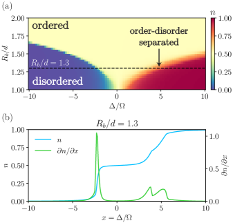
Figure 11: Mean field phase diagram of Hamiltonian (1) with $C_{6}$ coefficients from the first line of Table 2. (a) The excitation density $n$ depecited here is calculated using the optimized mean-field variational parameters $n=\frac{1}{L}\sum_{i=0}^{L-1}n_{i}$. (b) We also calculate $n$ and its derivative $\partial n/\partial x$ along the black dashed line ($R_{b}/d=1.3$) in (a) and $x\equiv\Delta/\Omega$ here.

For the paramters with the $\ket{111000\cdots}$ phase, it is better to choose $L=12$ than $L=6$ because the state $\ket{1110\cdots}$ cannot be faithfully represented in the unit cell of length 6. Since the eigendecomposition of the Hamiltonian matrix with a $L=12$ unit cell is time consuming, we compromise and calculate the phase diagram using $L=6$, as shown in Fig. 12(a), where only the boundary of the half-filling phase ($\ket{111000\cdots}$) and $3/4$-filling phase ($\ket{1110\cdots}$) is inconsistent with the DMRG result. We note that this disagreement is caused by the improper choice of the unit cell size. By taking $L=12$, we reexamine one case by scanning $R_{b}/d$ at fixed $\Delta/\Omega=5$, it is quite clear that once the unit cell size is properly chosen, the mean-field theory result is highly consistent with that from DMRG, as seen by the comparison in Fig. 12(b).

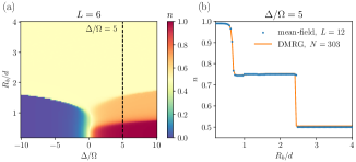
Figure 12: (a) Mean field phase diagram of Hamiltonian (1) with $C_{6}$ coefficients from the second line of Table 2. The order parameter depecited here is calculated using the optimized mean-field variational parameters $\langle n_{i}\rangle=\frac{1}{L}\sum_{i=0}^{L-1}n_{i}$. (b) The order parameter $\langle n_{i}\rangle$ calculated using mean-field theory with unit cell size $L=12$ along the black dashed line ($\Delta/\Omega=5$) is consistent with the DMRG calculations.

Appendix E Details on the calculation of level spacings

There are three(two) kinds of symmetry operations in the atom array with system $N=4n,n\in\mathbb{N}^{+}$($N=4n+2,n\in\mathbb{N}^{+}$) denoted $\hat{T}$, $\hat{P}_{AA}$ and $\hat{P}_{BB}$($\hat{T},\hat{P}_{AB}$) respectively. Their physical meaning is depicted in Fig. 13.

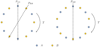
Figure 13: Symmetry operations in the two-species Rydberg atoms array under PBC for system size $N=4n,n\in\mathbb{N}^{+}$(left) and $N=4n+2,n\in\mathbb{N}^{+}$(right) are depicted above where the blue(yellow) circle stands for type A(B) atom.

We focus on the $N=4n$ ($n\in\mathbb{N}^{+}$) system. To calculate the level spacing distribution, we have to reduce all the symmetries in the system. For the caculation in the main text, we choose to diagonalize the system Hamiltonian in $k=0$ and $p_{AA}=p_{BB}=+1$ sector, i.e., translational invariant and inversion even sector. One can note that these three symmetry operations do not commute with one another indicating they do not have common eigenstates. However, it can be proved that within the $k=0$ subspace the three symmetry operations all commute or, more formally, all the translational invariant states

$$\ket{k_{a}}=\frac{1}{\sqrt{N_{a}}}\sum_{r=0}^{K-1}\hat{T}^{r}\ket{a}$$ (23)

fall into the kernal of the commutator of arbitary two operations out of three, where we use $\ket{k_{a}}$ to denote the momentum zero eigenstates, $\ket{a}$ to denote product states in computational basis, $K=N/2$ to denote the number of unit cell and $\sqrt{N_{a}}$ is the normalization coefficient.

The proof is quite direct. Considering an arbitrary computational basis $\ket{a}=|i_{0}i_{1}i_{2}\cdots i_{N-1}\rangle$, the outcome states acted on by symmetry operations $\hat{T},\hat{P}_{AA},\hat{P}_{BB}$ are

$$\hat{T}\ket{i_{0}i_{1}i_{2}\cdots i_{N-1}} = \ket{i_{N-2}i_{N-1}i_{0}\cdots i_{N-3}}$$ (24)

$$\hat{P}_{AA}\ket{i_{0}i_{1}i_{2}\cdots i_{N-1}} = \ket{i_{0}i_{N-1}i_{N-2}\cdots i_{1}}$$ (25)

$$\hat{P}_{BB}\ket{i_{0}i_{1}i_{2}\cdots i_{N-1}} = \ket{i_{2}i_{1}i_{0}i_{N-1}\cdots i_{3}}$$ (26)

respectively from which it is easy to obtain the following relation

$$\hat{P}_{AA}\hat{T} = \hat{T}^{-1}\hat{P}_{AA}$$ (27)

$$\hat{P}_{BB}\hat{T} = \hat{T}^{-1}\hat{P}_{BB}$$ (28)

$$\hat{T} = \hat{P}_{BB}\hat{P}_{AA}.$$ (29)

Therefore, for any translational invariant states, one can find

$$[\hat{P}_{AA},\hat{T}]\ket{k_{a}} = \hat{P}_{AA}\hat{T}\ket{k_{a}}-\hat{T}\hat{P}_{AA}\ket{k_{a}}$$ (30)

$$= \hat{P}_{AA}\hat{T}\ket{k_{a}}-\hat{P}_{AA}\hat{T}^{-1}\ket{k_{a}}=0$$ (31)

and similarly $[\hat{P}_{BB},\hat{T}]\ket{k_{a}}=0$ where we use $\hat{T}\ket{k_{a}}=\hat{T}^{-1}\ket{k_{a}}=\ket{k_{a}}$ because $\{\ket{k_{a}}\}$ are translational invariant states. Due to the same reason, the following equation is also true.

$$[\hat{P}_{AA},\hat{P}_{BB}]\ket{k_{a}}=\hat{T}^{-1}\ket{k_{a}}-\hat{T}\ket{k_{a}}=0$$ (32)

So by symmetrizing as follows

$$\ket{k_{a},p_{AA},p_{BB}}=\frac{1}{\mathcal{N}_{a}}(\mathbb{I}+\hat{P}_{AA})(\mathbb{I}+\hat{P}_{BB})\ket{k_{a}}$$ (33)

we can get the basis states in $k=0$ and $p_{AA}=p_{BB}=+1$ sector where $1/\mathcal{N}_{a}$ is only a normalization factor. Similarly, it can be concluded that $[\hat{P}_{AB},\hat{T}]\ket{k_{a}}=0$ in the $N=4n+2$ system.

For system with $N=16$, there are $4371$ basis states in the $k=0,p_{AA}=p_{BB}=+1$ symmetry sector after which the symmetry reduced Hamiltonian $H_{r}=UHU^{\dagger}$ can be directly decompose to obtain the eigenvalues where each column of $U$ corresponds to a specific $\ket{k_{a}}$ in the computational basis.

Appendix F Constructions of approximate quantum many-body scars

In the theoretical consideration, we only retain interactions between atoms separated by up to two atom spacings, which means only the nearest and next nearest interactions will be taken into consideration. We first map the Rydberg system Hamiltonian (1) to the quantum Ising model Hamiltonian using $\hat{n}_{i}=(\mathbb{I}+\hat{\sigma}_{i}^{z})/2$ and then one obtains Eq. (34),

$$\hat{H}=\frac{\Omega}{2}\left(\sum_{i}\hat{\sigma}_{2i}^{x}+\hat{\sigma}_{2i+1}^{x}\right)+\frac{V_{AA}}{4}\sum_{i}\hat{\sigma}_{2i}^{z}\hat{\sigma}^{z}_{2i+2}+\frac{V_{BB}}{4}\sum_{i}\hat{\sigma}_{2i+1}^{z}\hat{\sigma}^{z}_{2i+3}+\frac{V_{AB}}{4}\left(\sum_{i}\hat{\sigma}_{2i}^{z}\hat{\sigma}^{z}_{2i+1}+\hat{\sigma}_{2i+1}^{z}\hat{\sigma}^{z}_{2i+2}\right)$$

$$-\frac{1}{2}(\Delta-V_{AA}-V_{AB})\sum_{i}\hat{\sigma}_{2i}^{z}-\frac{1}{2}(\Delta-V_{BB}-V_{AB})\sum_{i}\hat{\sigma}_{2i+1}^{z}+\frac{N}{8}(V_{AA}+V_{BB}+2V_{AB}-4\Delta)\mathbb{I}.$$ (34)

where $V_{AA}=C_{AA}/(2d)^{6}$, $V_{BB}=C_{BB}/(2d)^{6}$ and $V_{AB}=C_{AB}/d^{6}$. To further simplify the Hamiltonian, we take some approximations. From now on, we only consider the situation where $V_{AA}=V_{BB}$ and the $\Delta$ is approriately chosen such that single $\hat{\sigma}^{z}_{i}$ term vanishes, i.e., $\Delta-V_{AA}-V_{AB}=0$ and $\Delta-V_{BB}-V_{AB}=0$. Therefore, the two-species Rydberg atoms array Hamiltonian is simplified into the quantum ANNNI model Hamiltonian. We denote the nearest interaction strength $V_{1}=V_{AB}/4$ as well as the next nearest interaction strength $V_{2}=V_{AA}/4=V_{BB}/4$, and then the simplified Hamiltonian writes

$$\hat{H}_{\mathrm{ANNNI}}=\frac{\Omega}{2}\sum_{n}\hat{\sigma}^{x}_{n}+V_{1}\sum_{n}\hat{\sigma}^{z}_{n}\hat{\sigma}^{z}_{n+1}+V_{2}\sum_{n}\hat{\sigma}_{n}^{z}\hat{\sigma}^{z}_{n+2}$$ (35)

where the integrability breaks due to the next nearest interaction term which can be proved by the level spacing indicator $\langle\tilde{r}_{i}\rangle$ in Fig. 14(a).

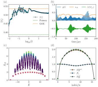
Figure 14: Numerical results for ANNNI model with system size $N=16$ and coefficients in Hamiltonian (35) are $(\Omega,V_{1},V_{2})=(2,-0.062,0.074)$. (a) The level spacing indicator $\langle\tilde{r}_{i}\rangle$ as a function of $\log_{10}\Omega$ in the symmetry reduced sector reveals that when $\Omega\gtrsim 0.1$ the system behaves in a chaotic way even if $\Omega$ is very large ($\Omega>10$). (b) Quench dynamics of the ANNNI model from $\ket{\mathbb{Z}_{2}}$ also shows non-thermaling behavior similar to the two-species Rydberg atoms array. (c) The eigenstates’ energy-entanglement spectrum is similar to the two-species Rydberg atoms array, where they both unfold low bipatite entanglement entropy eigenstates with the same arch structure. (d) Fidelity and bipartite entanglement entropy of the states constructed by the quasiparticle operator $\hat{\beta}_{k}^{\dagger}$ are compared with the exact eigenstates obtained via numerical method. Here, the fidelity $\mathcal{F}_{n}$ is defined as the overlap between exact state $\ket{s_{n}}$ and constructed state $\ket{s_{n}^{\prime}}$, i.e., $\mathcal{F}_{n}=|\langle s_{n}|s_{n}^{\prime}\rangle|^{2}$. The bipartite entanglement entropy of the mean field states $S_{\mathrm{vN}}^{\mathrm{mf}}$ are very close to the entropy of the exact results $S_{\mathrm{vN}}^{\mathrm{exact}}$.

First, we perform local unitary transformation followed by the Jordan-Wigner transformation such that $\hat{\sigma}^{x}\leftrightarrow\hat{\sigma}^{z}$ and the same Hamiltonian written in spinless fermion operators can be obtained (Eq. (36)).

$$\hat{H}_{\mathrm{JW}}=\Omega\sum_{n}\hat{c}_{n}^{\dagger}\hat{c}_{n}+V_{1}\sum_{n}(\hat{c}_{n}-\hat{c}_{n}^{\dagger})(\hat{c}_{n+1}^{\dagger}+\hat{c}_{n+1})$$

$$+V_{2}\sum_{n}(\hat{c}_{n}-\hat{c}_{n}^{\dagger})(2\hat{c}_{n+1}^{\dagger}\hat{c}_{n+1}-1)(\hat{c}_{n+2}^{\dagger}+\hat{c}_{n+2})$$ (36)

Second, mean-field approximation can be applied. We define

$$\alpha = \langle 2\hat{c}_{n+1}^{\dagger}\hat{c}_{n+1}-1\rangle=\braket{\hat{\sigma}^{z}_{n+1}}$$ (37)

$$\mu = \langle(\hat{c}_{n}^{\dagger}-\hat{c}_{n})(\hat{c}_{n+2}^{\dagger}+\hat{c}_{n+2})\rangle$$ (38)

$$= \braket{\hat{\sigma}^{x}_{n}\hat{\sigma}^{z}_{n+1}\hat{\sigma}^{x}_{n+2}}$$ (39)

and denote $\tilde{\Omega}=\Omega+2\mu V_{2}$ as well as $\tilde{V}_{2}=\alpha V_{2}$, and then the mean-field Hamiltonian $\hat{H}_{\mathrm{MF}}$ reads (ignoring a constant)

$$\hat{H}_{\mathrm{MF}} = \tilde{\Omega}\sum_{n}\hat{c}_{n}^{\dagger}\hat{c}_{n}+V_{1}\sum_{n}(\hat{c}_{n}-\hat{c}_{n}^{\dagger})(\hat{c}_{n+1}^{\dagger}+\hat{c}_{n+1})$$ (40)

$$+\tilde{V}_{2}\sum_{n}(\hat{c}_{n}-\hat{c}_{n}^{\dagger})(\hat{c}_{n+2}^{\dagger}+\hat{c}_{n+2})$$

where it has to be emphasized that the mean-field Hamiltonian $\hat{H}_{\mathrm{MF}}$ possesses fermion parity conservation which naturally gives rise to the two different symmetry sectors with even and odd parity. Different symmetry sectors correspond with different boundary conditions. The even(odd) parity $p=0$ ($p=1$) is associated with the PBC(ABC), which is clearly shown in Eq.(41),

$$\hat{c}_{N}=(-1)^{p}\hat{c}_{0}$$ (41)

where we use 0 to label the first atom. The $p=0$ ($p=1$) sector indicates $e^{ikN}=1$ ($e^{ikN}=-1$) and thus the choice of wave vector $k$ given by PBC (ABC) is $\mathcal{K}^{\mathrm{ABC}}_{p=0}$ ($\mathcal{K}^{\mathrm{PBC}}_{p=1}$)

$$\mathcal{K}^{\mathrm{PBC}}_{p=0} = \left\{k=\frac{2m\pi}{N},m=-\frac{N}{2}+1,\cdots,\frac{N}{2}\right\}$$ (42)

$$\mathcal{K}^{\mathrm{ABC}}_{p=1} = \left\{k=\pm\frac{(2m-1)\pi}{N},m=1,\cdots,\frac{N}{2}\right\}$$ (43)

where $m\in\mathbb{Z}$. Next, we obtain the energy spectrum using Fourier transformation.

$$\hat{c}_{n} = \frac{1}{\sqrt{N}}\sum_{k}e^{-ikn}\hat{c}_{k}$$ (44)

$$\hat{c}_{n}^{\dagger} = \frac{1}{\sqrt{N}}\sum_{k}e^{ikn}\hat{c}_{k}^{\dagger}$$ (45)

After defining

$$A = \tilde{\Omega}-2V_{1}\cos k-2\tilde{V}_{2}\cos 2k$$ (46)

$$B = 2(V_{1}\sin k+\tilde{V}_{2}\sin 2k)$$ (47)

$$C = \sqrt{A^{2}+B^{2}}$$ (48)

the Hamiltonian in momentum space can be written in a simple form

$$\hat{H}_{\mathrm{MF}}=\sum_{k}\begin{pmatrix}\hat{c}_{k}^{\dagger}&\hat{c}_{-k}\end{pmatrix}\begin{pmatrix}A&iB\\ -iB&-A\end{pmatrix}\begin{pmatrix}\hat{c}_{k}\\ \hat{c}^{\dagger}_{-k}\end{pmatrix}$$ (49)

and the dipersion relation is $\epsilon_{k}=\pm C$.

To construct the quasipaticle operator $\hat{\beta}_{k}^{\dagger}$, we use the Bogoliubov transformation

$$\begin{pmatrix}\hat{\beta}_{k}\\ \hat{\beta}_{-k}^{\dagger}\end{pmatrix}=\begin{pmatrix}u_{k}&-v_{k}\\ v_{k}^{*}&u_{k}^{*}\end{pmatrix}\begin{pmatrix}\hat{c}_{k}\\ \hat{c}_{-k}^{\dagger}\end{pmatrix}$$ (50)

where $u_{k}$ is real and $v_{k}$ is purely imaginary

$$u_{k}=\frac{A+C}{\sqrt{2C(A+C)}};\ v_{k}=\frac{-iB}{\sqrt{2C(A+C)}}$$ (51)

and the Hamiltonian in the language of quasiparticle operators reads

$$\hat{H}_{\mathrm{MF}}=\sum_{k}\epsilon_{k}(\hat{\beta}_{k}^{\dagger}\hat{\beta}_{k}+\hat{\beta}_{-k}^{\dagger}\hat{\beta}_{-k}-1)$$ (52)

from which the ground state can be directly deduced, i.e., the Bogoliubov vacuum $\ket{\emptyset}$ satisfying $\hat{\beta}_{k}\ket{\emptyset}=0,\forall k$. Here, we need to figure out which symmetry sector the real ground state falls into because there are two ground states, one ($\ket{\emptyset}^{\mathrm{ABC}}$) in the ABC sector and the other ($\ket{\emptyset}^{\mathrm{PBC}}$) in the PBC sector. It turns out that the real ground state falls into the ABC sector, indicating $\ket{\emptyset}^{\mathrm{ABC}}$ is the ground state of the whole system. The two ground states in terms of fermoin operators can be expressed

$$\ket{\emptyset}^{\mathrm{ABC}} = \prod_{k>0}^{\mathcal{K}^{\mathrm{ABC}}_{p=1}}\Big{(}u_{k}+v_{k}\hat{c}_{k}^{\dagger}\hat{c}_{-k}^{\dagger}\Big{)}\ket{0}$$ (53)

$$\ket{\emptyset}^{\mathrm{PBC}} = \hat{c}_{k=0}^{\dagger}\prod_{0<k<\pi}^{\mathcal{K}^{\mathrm{PBC}}_{p=0}}\Big{(}u_{k}+v_{k}\hat{c}_{k}^{\dagger}\hat{c}_{-k}^{\dagger}\Big{)}\ket{0}$$ (54)

where $\ket{0}$ is the fermion vacuum $\hat{c}_{k}\ket{0}=0,\forall k$ and $\hat{c}_{k=0}^{\dagger}$ is the creation operator of a fermion with zero momentum.

We found that the low bipartite entanglement entropy states $\ket{s_{n}}$ can be well contructed using states in Eq. (13) with $\sum_{k}n_{k}=\lfloor n/2\rfloor$. Specifically, we use $\ket{\psi_{\{n_{k}\}}^{\mathrm{ABC}/\mathrm{PBC}}}$ as the basis and numerically calculate the coefficient $c_{\{n_{k}\}}=\langle\psi_{\{n_{k}\}}^{p=n\ \mathrm{mod}\ 2}|s_{n}\rangle$ in Eq. (55),

$$\ket{s^{\prime}_{n}}=\frac{1}{\mathcal{N}}\sum_{\{n_{k}\}}^{\sum_{k}n_{k}=\lfloor n/2\rfloor}c_{\{n_{k}\}}\ket{\psi_{\{n_{k}\}}^{p=n\ \mathrm{mod}\ 2}}$$ (55)

where $\mathcal{N}$ is the normalization coefficent, $\ket{\psi_{\{n_{k}\}}^{p=0}}=\ket{\psi_{\{n_{k}\}}^{\mathrm{ABC}}}$ and $\ket{\psi_{\{n_{k}\}}^{p=1}}=\ket{\psi_{\{n_{k}\}}^{\mathrm{PBC}}}$.

In the following, we show some the numerical results. The ANNNI model has the similar eigenstate energy-entanglement spectrum with the two-species Rydberg atoms array which can be clearly seen in Fig. 14(c), where those dots marked with red circles are regarded as the approximate quantum many-body scars, which can be well captured by the basis shown in Eq. (55). For system of small size ($N=16$), the calculation results shows that the fidelity $\mathcal{F}_{n}=|\langle s_{n}^{\prime}|s_{n}\rangle|^{2}>0.89$ when the coefficients in the Hamiltonian are chosen to be $(\Omega,V_{1},V_{2})=(2,-0.062,0.074)$ and the variational parameters are chosen to be $(\alpha,\mu)=(2n/N-1,0)$. The fidelity $\mathcal{F}_{n}$ can also be interpreted as the average value of zero momentum subspace projector

$$\mathcal{F}_{n}=|\langle s_{n}|\hat{P}|s_{n}\rangle|^{2}$$ (56)

where

$$\hat{P} = \sum_{\{n_{k}\}}^{\sum_{k}n_{k}=\lfloor n/2\rfloor}\hat{P}_{\{n_{k}\}}$$ (57)

$$\hat{P}_{\{n_{k}\}} = \ket{\psi_{\{n_{k}\}}^{p=n\ \mathrm{mod}\ 2}}\langle\psi_{\{n_{k}\}}^{p=n\ \mathrm{mod}\ 2}|.$$ (58)

We note that one can optimize these mean-field variational parameters $(\alpha,\mu)$ to obtain higher fidelity.

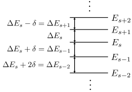
Figure 15: The energy levels of scar states exhibit decreasing energy level spacing with growing index $s$ or energy $E_{s}$. Here we define $\Delta E_{s}=E_{s+1}-E_{s}$.

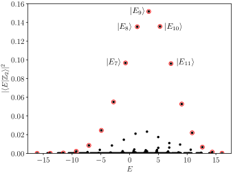
Figure 16: The overlap of $\ket{\mathbb{Z}_{2}}$ with all eigenstates is depicted where those marked with red circles are the ones with approximate scar states.

Figure 17: The eigenenergy of scar states $E_{s}$ and their neighbouring spacings $\Delta E_{s}=E_{s+1}-E_{s}$ are depicted in (a) and (b) respectively. The decreasing energy level spacings are visulized in Fig. 15.

Appendix G Discussion on the possible DQPT phenomenon

Figure 18: Loschmidt rate $\lambda(z)=-\frac{1}{N}|\langle\mathbb{Z}_{2}|e^{-i\hat{H}z}|\mathbb{Z}_{2}\rangle|^{2}$ over the complex plane is calculated for Rydberg atoms array with size $N=12$ where $(\Omega,\Delta,d)=(2,0.05,9)$ and the $C_{6}$ coefficients are chosen from the first line of Table 2. Those red dots around real axis are the possible zeros of Loschmidt amplitude in the thermodynamic limit and their number corresponds to the number of scar states in the system. Grey dashed line is the real axis and also the evolution path of the system.

Figure 19: Discussion on the non-analytical behavior of Loschmidt rate $\lambda(t)$. (a) The Loschmidt rate of $N=16$ system is calculated for both PBC and OBC and $\lambda_{S}(t)$ constructed using our bold approximations is also depicted here. It can be found that our $\lambda_{S}(t)$ corresponds well with the exact $\lambda(t)$ obtained via ED. (b) The first three time points $t_{1},t_{2},t_{3}$ where approximate Loschmidt rate $\lambda_{S}(t)$ shows non-analytical behavior are marked with grey dashed line in (a) and their relation with $\Delta E_{p}$ is depicted here.

We use numerical integration scheme to calculate the quench dynamics for small system and TDVP method for larger system. In both cases, the discontinous behavior of the Loschmidt rate can be easily identified as shown in Fig. 4(f).

Generally speaking, DQPT can be explained by the Lee-Yang zeros (also called Fisher zeros sometimes) of the Loschmidt amplitude $\mathcal{G}(z)=\bra{\psi_{0}}e^{-i\hat{H}z}\ket{\psi_{0}}$ in the complex plane, where $\ket{\psi_{0}}$ is the initial state , $z=t+i\tau$ is the complex time and we choose $\ket{\psi_{0}}=\ket{\mathbb{Z}_{2}}$ here. When $\mathcal{G}(z)\to 0$, the Loschmidt rate $\lambda(z)=-\frac{1}{N}\ln|\mathcal{G}(t)|^{2}$ will diverge and that is why $\lambda(t)$ becomes discontinous at some point. We calculated the $\lambda(z)$ over the complex plane as shown in Fig. 18 and found that those possible Lee-Yang zeros tend to form lines crossing the real axis with the system becoming larger and their number corresponds with the number of QMBS in the system. This phenomenon can be partially explained by the approximate QMBS we discussed above.

The initial state $\ket{\mathbb{Z}_{2}}$ can be formally decomposed by the eigenstates $\ket{E_{k}}$ and also can be approximately decomposed by the scar states $\ket{E_{s}}$ where we use $k$ to label general eigenstates and $s$ to label scar eigenstates,

$$\ket{\mathbb{Z}_{2}}=\sum_{k=0}^{2^{N}-1}c_{k}\ket{E_{k}}\approx\sum_{s=0}^{N}c_{s}\ket{E_{s}}$$ (59)

so the Loschmidt amplitude is

$$\mathcal{G}(t)=\bra{\mathbb{Z}_{2}}e^{-i\hat{H}t}\ket{\mathbb{Z}_{2}}=\sum_{s}|c_{s}|^{2}e^{-iE_{s}t}$$ (60)

and the corresponding Loschmidt echo $\mathcal{L}(t)=|\mathcal{G}(t)|^{2}$ is

$$\mathcal{L}(t)=\sum_{s,s^{\prime}}|c_{s}|^{2}|c_{s^{\prime}}|^{2}e^{-i(E_{s}-E_{s^{\prime}})t}.$$ (61)

The scar states in our system are approximiate so their energy level spacings are not equal, we consider the situation where $(E_{s+1}-E_{s})-(E_{s}-E_{s-1})=\delta$ is a constant as shown in Fig. (15).

To further simplify our discussion, we now only consider the contribution of five scar states $\{\ket{E_{s}},s=7,8,9,10,11\}$ (taking $N=16$ as an example here) to the system dynamics because they have the largest overlap with $\ket{\mathbb{Z}_{2}}$ which can be confirmed in Fig. 16. Hence the Eq. (61) approximately equals to

$$\mathcal{L}(t)\approx\sum_{s^{\prime}=7}^{10}\sum_{s=s^{\prime}}^{11}2|c_{s}|^{2}|c_{s^{\prime}}|^{2}\cos[(E_{s}-E_{s^{\prime}})t]$$ (62)

and from now on we will make bold approximations. We only consider the low frequency part of the Loschmidt echo in Eq. (62), which leads to the final expression for Loschmidt echo $\mathcal{L}_{S}(t)$

$$\mathcal{L}_{S}(t)=\sum_{s=7}^{10}2\Big{(}|c_{s}|^{2}|c_{s+1}|^{2}\cos\Delta E_{s}t+|c_{s}|^{4}\Big{)}$$ (63)

and the corresponding Loschmidt rate is

$$\lambda_{S}(t)=-\frac{1}{N_{S}}\ln\frac{\mathcal{L}(t)}{\mathcal{L}(0)}$$ (64)

where it’s not appropriate to let $N_{S}=N=16$ because only five states instead of all eigenstates are used to extract the dynamical property. We hence propose using $N_{S}=\log_{2}5$ to calculate $\lambda_{S}(t)$. We also slightly change the definition of Loschmidt rate to ensure $\lambda_{S}(0)=0$ still holds. Surprisingly, the dynamics of $\lambda_{S}(t)$ behaves very similar to the exact Loschmidt rate $\lambda(t)$ calculated using ED method as shown in Fig. 19(a).

The Eq. (64) can also be used to explain why the red dots (approximate zeros of Loschmidt amplitude) form a sloping line as shown in Fig. 18. This is because the initial state at $t=0$ has different energy with varying $\tau$, or put it in another way, the overlap between $e^{\hat{H}\tau}\ket{\mathbb{Z}_{2}}$ (not normalized) and eigenstates (especially the scar states) has a different peak so the energy level spacing $\Delta E_{s}$, $\delta$ and the corresponding $|c_{s}|^{2}$ will change and they certainly will follow the index $s$ of the scar state who has the largest overlap with initial state $e^{\hat{H}\tau}\ket{\mathbb{Z}_{2}}$. To keep the discussion simple, we assume the ratio between $|c_{s}|^{2}$ as well as $\delta$ will not change (much) and only consider the effect that different $\Delta E_{s}$ may take. Now we only need to calculate the first zero (besides $t=0$) of the derivative of $\mathcal{L}_{S}(t)$ since it corresponds to the first non-analytical point of $\lambda_{S}(t)$. The derivative of $\mathcal{L}_{S}(t)$ takes the following form

$$\frac{\mathrm{d}\mathcal{L}_{S}(t)}{\mathrm{d}t}=-2\sum_{s=p-2}^{p+1}|c_{s}|^{2}|c_{s+1}|^{2}\Delta E_{s}\sin\Delta E_{s}t$$ (65)

where we use $p$ to denote the index of scar state who has the largest overlap with the initial state $e^{\hat{H}\tau}\ket{\mathbb{Z}_{2}}$. The relation between $\Delta E_{p}$ and the first, third and fifth zero $\lambda_{S}(t)$ (denoted $t_{1},t_{2}$ and $t_{3}$ respectively) of $\mathrm{d}\mathcal{L}_{S}(t)/\mathrm{d}t$ is shown in Fig. 19(b).

The negative correlation between $t_{1},t_{2},t_{3}$ and $\Delta E_{p}$ and can be clearly seen in Fig. 19(b) and $\Delta E_{p}$ as well as $p$ also exhibit anticorrelation as shown in Fig. 17(b). Therefore, in conclusion, as $\tau$ increases, the energy of $e^{\hat{H}\tau}\ket{\mathbb{Z}_{2}}$ will increase and it leads to the rise in $p$ which further causes the decrease of $\Delta E_{p}$ and consequently $t_{1},t_{2},t_{3}$ increases. Hence for a single branch of red dots, smaller $\tau$ always corresponds to smaller $t$ and this can be explained using our approximate Loschmidt rate $\lambda_{S}(t)$ in a phenomenological way.

Due to the similarity between the two-species Rydberg atom array and quantum ANNNI model, we claim that the above discussion on the relation between QMBS and DQPT can also be applied to the quench dynamics of the quantum ANNNI model, i.e., we can use QMBS to explain the DQPT in the quantum ANNNI model which has already been studied numerically in detail [57].

References

- Urban et al. [2009] E. Urban, T. A. Johnson, T. Henage, L. Isenhower, D. D. Yavuz, T. G. Walker, and M. Saffman, Observation of rydberg blockade between two atoms, Nature Physics 5, 110 (2009).
- Browaeys and Lahaye [2020] A. Browaeys and T. Lahaye, Many-body physics with individually controlled rydberg atoms, Nature Physics 16, 132 (2020).
- Keesling et al. [2019] A. Keesling, A. Omran, H. Levine, H. Bernien, H. Pichler, S. Choi, R. Samajdar, S. Schwartz, P. Silvi, S. Sachdev, P. Zoller, M. Endres, M. Greiner, V. Vuletić, and M. D. Lukin, Quantum kibble–zurek mechanism and critical dynamics on a programmable rydberg simulator, Nature 568, 207 (2019).
- Lienhard et al. [2018] V. Lienhard, S. de Léséleuc, D. Barredo, T. Lahaye, A. Browaeys, M. Schuler, L.-P. Henry, and A. M. Läuchli, Observing the space- and time-dependent growth of correlations in dynamically tuned synthetic ising models with antiferromagnetic interactions, Phys. Rev. X 8, 021070 (2018).
- Kim et al. [2024] K. Kim, F. Yang, K. Mølmer, and J. Ahn, Realization of an extremely anisotropic heisenberg magnet in rydberg atom arrays, Phys. Rev. X 14, 011025 (2024).
- Kalinowski et al. [2023] M. Kalinowski, N. Maskara, and M. D. Lukin, Non-abelian floquet spin liquids in a digital rydberg simulator, Phys. Rev. X 13, 031008 (2023).
- Evered et al. [2023] S. J. Evered, D. Bluvstein, M. Kalinowski, S. Ebadi, T. Manovitz, H. Zhou, S. H. Li, A. A. Geim, T. T. Wang, N. Maskara, H. Levine, G. Semeghini, M. Greiner, V. Vuletić, and M. D. Lukin, High-fidelity parallel entangling gates on a neutral-atom quantum computer, Nature 622, 268 (2023).
- Theis et al. [2016] L. S. Theis, F. Motzoi, F. K. Wilhelm, and M. Saffman, High-fidelity rydberg-blockade entangling gate using shaped, analytic pulses, Phys. Rev. A 94, 032306 (2016).
- Fu et al. [2022] Z. Fu, P. Xu, Y. Sun, Y.-Y. Liu, X.-D. He, X. Li, M. Liu, R.-B. Li, J. Wang, L. Liu, and M.-S. Zhan, High-fidelity entanglement of neutral atoms via a rydberg-mediated single-modulated-pulse controlled-phase gate, Phys. Rev. A 105, 042430 (2022).
- Bluvstein et al. [2024] D. Bluvstein, S. J. Evered, A. A. Geim, S. H. Li, H. Zhou, T. Manovitz, S. Ebadi, M. Cain, M. Kalinowski, D. Hangleiter, J. P. Bonilla Ataides, N. Maskara, I. Cong, X. Gao, P. Sales Rodriguez, T. Karolyshyn, G. Semeghini, M. J. Gullans, M. Greiner, V. Vuletić, and M. D. Lukin, Logical quantum processor based on reconfigurable atom arrays, Nature 626, 58 (2024).
- Pause et al. [2024] L. Pause, L. Sturm, M. Mittenbühler, S. Amann, T. Preuschoff, D. Schäffner, M. Schlosser, and G. Birkl, Supercharged two-dimensional tweezer array with more than 1000 atomic qubits, Optica 11, 222 (2024).
- Bernien et al. [2017] H. Bernien, S. Schwartz, A. Keesling, H. Levine, A. Omran, H. Pichler, S. Choi, A. S. Zibrov, M. Endres, M. Greiner, V. Vuletić, and M. D. Lukin, Probing many-body dynamics on a 51-atom quantum simulator, Nature 551, 579 (2017).
- Zhang et al. [2024] J. Zhang, S. H. Cantú, F. Liu, A. Bylinskii, B. Braverman, F. Huber, J. Amato-Grill, A. Lukin, N. Gemelke, A. Keesling, S.-T. Wang, Y. Meurice, and S. W. Tsai, Probing quantum floating phases in rydberg atom arrays (2024), arXiv:2401.08087 [quant-ph] .
- Ebadi et al. [2021] S. Ebadi, T. T. Wang, H. Levine, A. Keesling, G. Semeghini, A. Omran, D. Bluvstein, R. Samajdar, H. Pichler, W. W. Ho, S. Choi, S. Sachdev, M. Greiner, V. Vuletić, and M. D. Lukin, Quantum phases of matter on a 256-atom programmable quantum simulator, Nature 595, 227 (2021).
- Samajdar et al. [2020] R. Samajdar, W. W. Ho, H. Pichler, M. D. Lukin, and S. Sachdev, Complex density wave orders and quantum phase transitions in a model of square-lattice rydberg atom arrays, Phys. Rev. Lett. 124, 103601 (2020).
- Samajdar et al. [2021] R. Samajdar, W. W. Ho, H. Pichler, M. D. Lukin, and S. Sachdev, Quantum phases of rydberg atoms on a kagome lattice, Proceedings of the National Academy of Sciences 118, e2015785118 (2021), https://www.pnas.org/doi/pdf/10.1073/pnas.2015785118 .
- Celi et al. [2020] A. Celi, B. Vermersch, O. Viyuela, H. Pichler, M. D. Lukin, and P. Zoller, Emerging two-dimensional gauge theories in rydberg configurable arrays, Phys. Rev. X 10, 021057 (2020).
- de Léséleuc et al. [2019] S. de Léséleuc, V. Lienhard, P. Scholl, D. Barredo, S. Weber, N. Lang, H. P. Büchler, T. Lahaye, and A. Browaeys, Observation of a symmetry-protected topological phase of interacting bosons with rydberg atoms, Science 365, 775 (2019), https://www.science.org/doi/pdf/10.1126/science.aav9105 .
- Wu et al. [2024] X. Wu, Z. Wang, F. Yang, R. Gao, C. Liang, M. K. Tey, X. Li, T. Pohl, and L. You, Dissipative time crystal in a strongly interacting rydberg gas, Nature Physics 10.1038/s41567-024-02542-9 (2024).
- Fan et al. [2020] C.-h. Fan, D. Rossini, H.-X. Zhang, J.-H. Wu, M. Artoni, and G. C. La Rocca, Discrete time crystal in a finite chain of rydberg atoms without disorder, Phys. Rev. A 101, 013417 (2020).
- Liu et al. [2024] B. Liu, L.-H. Zhang, Y. Ma, T.-Y. Han, Q.-F. Wang, J. Zhang, Z.-Y. Zhang, S.-Y. Shao, Q. Li, H.-C. Chen, Y.-J. Wang, J.-D. Nan, Y.-M. Yin, D.-S. Ding, and B.-S. Shi, Microwave seeding time crystal in floquet driven rydberg atoms (2024), arXiv:2404.12180 [cond-mat.quant-gas] .
- Hauke and Heyl [2015] P. Hauke and M. Heyl, Many-body localization and quantum ergodicity in disordered long-range ising models, Phys. Rev. B 92, 134204 (2015).
- Bluvstein et al. [2021] D. Bluvstein, A. Omran, H. Levine, A. Keesling, G. Semeghini, S. Ebadi, T. T. Wang, A. A. Michailidis, N. Maskara, W. W. Ho, S. Choi, M. Serbyn, M. Greiner, V. Vuletić, and M. D. Lukin, Controlling quantum many-body dynamics in driven rydberg atom arrays, Science 371, 1355 (2021), https://www.science.org/doi/pdf/10.1126/science.abg2530 .
- Turner et al. [2018a] C. J. Turner, A. A. Michailidis, D. A. Abanin, M. Serbyn, and Z. Papić, Quantum scarred eigenstates in a rydberg atom chain: Entanglement, breakdown of thermalization, and stability to perturbations, Phys. Rev. B 98, 155134 (2018a).
- Choi et al. [2019] S. Choi, C. J. Turner, H. Pichler, W. W. Ho, A. A. Michailidis, Z. Papić, M. Serbyn, M. D. Lukin, and D. A. Abanin, Emergent su(2) dynamics and perfect quantum many-body scars, Phys. Rev. Lett. 122, 220603 (2019).
- Serbyn et al. [2021a] M. Serbyn, D. A. Abanin, and Z. Papić, Quantum many-body scars and weak breaking of ergodicity, Nature Physics 17, 675 (2021a).
- Turner et al. [2018b] C. J. Turner, A. A. Michailidis, D. A. Abanin, M. Serbyn, and Z. Papić, Weak ergodicity breaking from quantum many-body scars, Nature Physics 14, 745 (2018b).
- Rader and Läuchli [2019] M. Rader and A. M. Läuchli, Floating phases in one-dimensional rydberg ising chains (2019), arXiv:1908.02068 [cond-mat.quant-gas] .
- Cea et al. [2024] M. Cea, M. Grossi, S. Monaco, E. Rico, L. Tagliacozzo, and S. Vallecorsa, Exploring the phase diagram of the quantum one-dimensional annni model (2024), arXiv:2402.11022 [cond-mat.str-el] .
- Rieger and Uimin [1996] H. Rieger and G. Uimin, The one-dimensional annni model in a transverse field: analytic and numerical study of effective hamiltonians, Zeitschrift für Physik B Condensed Matter 101, 597–611 (1996).
- Fisher and Selke [1980] M. E. Fisher and W. Selke, Infinitely many commensurate phases in a simple ising model, Phys. Rev. Lett. 44, 1502 (1980).
- Šibalić et al. [2017] N. Šibalić, J. Pritchard, C. Adams, and K. Weatherill, Arc: An open-source library for calculating properties of alkali rydberg atoms, Computer Physics Communications 220, 319 (2017).
- White [1992] S. R. White, Density matrix formulation for quantum renormalization groups, Phys. Rev. Lett. 69, 2863 (1992).
- Fishman et al. [2022a] M. Fishman, S. R. White, and E. M. Stoudenmire, The ITensor Software Library for Tensor Network Calculations, SciPost Phys. Codebases , 4 (2022a).
- Fishman et al. [2022b] M. Fishman, S. R. White, and E. M. Stoudenmire, Codebase release 0.3 for ITensor, SciPost Phys. Codebases , 4 (2022b).
- Chepiga and Mila [2021] N. Chepiga and F. Mila, Lifshitz point at commensurate melting of chains of rydberg atoms, Phys. Rev. Res. 3, 023049 (2021).
- White et al. [2002] S. R. White, I. Affleck, and D. J. Scalapino, Friedel oscillations and charge density waves in chains and ladders, Phys. Rev. B 65, 165122 (2002).
- [38] A follow-up paper is under preparation where we will discuss the abovementioned low energy effective Hamiltonian and the relation between and at length.
- Affleck and Ludwig [1991] I. Affleck and A. W. W. Ludwig, Universal noninteger “ground-state degeneracy” in critical quantum systems, Phys. Rev. Lett. 67, 161 (1991).
- Vidal et al. [2003] G. Vidal, J. I. Latorre, E. Rico, and A. Kitaev, Entanglement in quantum critical phenomena, Phys. Rev. Lett. 90, 227902 (2003).
- Holzhey et al. [1994] C. Holzhey, F. Larsen, and F. Wilczek, Geometric and renormalized entropy in conformal field theory, Nuclear Physics B 424, 443 (1994).
- Calabrese and Cardy [2004] P. Calabrese and J. Cardy, Entanglement entropy and quantum field theory, Journal of Statistical Mechanics: Theory and Experiment 2004, P06002 (2004).
- Sørensen et al. [2007] E. S. Sørensen, M.-S. Chang, N. Laflorencie, and I. Affleck, Quantum impurity entanglement, Journal of Statistical Mechanics: Theory and Experiment 2007, P08003 (2007).
- Calabrese and Cardy [2009] P. Calabrese and J. Cardy, Entanglement entropy and conformal field theory, Journal of Physics A: Mathematical and Theoretical 42, 504005 (2009).
- Allen et al. [2001] D. Allen, P. Azaria, and P. Lecheminant, A two-leg quantum ising ladder: a bosonization study of the annni model, Journal of Physics A: Mathematical and General 34, L305–L310 (2001).
- Pollmann et al. [2009] F. Pollmann, S. Mukerjee, A. M. Turner, and J. E. Moore, Theory of finite-entanglement scaling at one-dimensional quantum critical points, Phys. Rev. Lett. 102, 255701 (2009).
- Zauner-Stauber et al. [2018] V. Zauner-Stauber, L. Vanderstraeten, M. T. Fishman, F. Verstraete, and J. Haegeman, Variational optimization algorithms for uniform matrix product states, Phys. Rev. B 97, 045145 (2018).
- Deutsch [1991] J. M. Deutsch, Quantum statistical mechanics in a closed system, Phys. Rev. A 43, 2046 (1991).
- Srednicki [1994] M. Srednicki, Chaos and quantum thermalization, Phys. Rev. E 50, 888 (1994).
- Luca D’Alessio and Rigol [2016] A. P. Luca D’Alessio, Yariv Kafri and M. Rigol, From quantum chaos and eigenstate thermalization to statistical mechanics and thermodynamics, Advances in Physics 65, 239 (2016).
- Abanin et al. [2019] D. A. Abanin, E. Altman, I. Bloch, and M. Serbyn, Colloquium: Many-body localization, thermalization, and entanglement, Rev. Mod. Phys. 91, 021001 (2019).
- Serbyn et al. [2021b] M. Serbyn, D. A. Abanin, and Z. Papić, Quantum many-body scars and weak breaking of ergodicity, Nature Physics 17, 675 (2021b).
- Atas et al. [2013] Y. Y. Atas, E. Bogomolny, O. Giraud, and G. Roux, Distribution of the ratio of consecutive level spacings in random matrix ensembles, Phys. Rev. Lett. 110, 084101 (2013).
- Heyl [2018] M. Heyl, Dynamical quantum phase transitions: a review, Reports on Progress in Physics 81, 054001 (2018).
- Rach et al. [2015] N. Rach, M. M. Müller, T. Calarco, and S. Montangero, Dressing the chopped-random-basis optimization: A bandwidth-limited access to the trap-free landscape, Phys. Rev. A 92, 062343 (2015).
- Müller et al. [2022] M. M. Müller, R. S. Said, F. Jelezko, T. Calarco, and S. Montangero, One decade of quantum optimal control in the chopped random basis, Reports on Progress in Physics 85, 076001 (2022).
- Karrasch and Schuricht [2013] C. Karrasch and D. Schuricht, Dynamical phase transitions after quenches in nonintegrable models, Phys. Rev. B 87, 195104 (2013).