SLAM2REF: Advancing Long-Term Mapping with 3D LiDAR and Reference Map Integration for Precise 6-DoF Trajectory Estimation and Map Extension

Abstract

This paper presents a pioneering solution to the task of integrating mobile 3D LiDAR and inertial measurement unit (IMU) data with existing building information models or point clouds, which is crucial for achieving precise long-term localization and mapping in indoor, GPS-denied environments. Our proposed framework, SLAM2REF, introduces a novel approach for automatic alignment and map extension utilizing reference 3D maps. The methodology is supported by a sophisticated multi-session anchoring technique, which integrates novel descriptors and registration methodologies. Real-world experiments reveal the framework’s remarkable robustness and accuracy, surpassing current state-of-the-art methods. Our open-source framework’s significance lies in its contribution to resilient map data management, enhancing processes across diverse sectors such as construction site monitoring, emergency response, disaster management, and others, where fast-updated digital 3D maps contribute to better decision-making and productivity. Moreover, it offers advancements in localization and mapping research. Link to the repository: https://github.com/MigVega/SLAM2REF, Data: https://doi.org/10.14459/2024mp1743877 .

1 Introduction

Nowadays, mobile mapping systems incorporated into mobile robots or handheld devices equipped with sensors and applying state-of-the-art SLAM algorithms allow the quick creation of updated 3D maps. However, these maps are in their local coordinates systems and, therefore, separated from any prior information. Additionally, they might contain potential drift issues, rendering them unsuitable for comparative analysis or change detection.

Several real-world applications require the capacity to align, compare, and manage 3D data received at various intervals that may be separated by lengthy intervals of time. This process is referred to as long-term map management.

Long-term map management is crucial since the real world constantly evolves and changes. This applies to humans who want to utilize the map to comprehend the current situation and its evolution and to autonomous robots for effective and fast navigation.

Moreover, achieving accurate alignment and effective management of extensive datasets represent significant challenges in enabling the creation of DTs (DTs) for cities and buildings [2, 58]. As explained by [10], in complex implementations, automatic alignment of 3D data becomes imperative to achieve DTs with maturity levels of 3 or higher. Such levels necessitate the augmentation of models with a continuous flow of real-world information.

An automatic map alignment and change detection pipeline also contribute to the seamless integration of mapping devices into existing workflows in the industry. A recent survey revealed that the compatibility of mapping devices with existing tools is, after the budget, the second most crucial barrier surrounding the usage of mobile mapping devices [62].

For example, an up-to-date 3D digital map can help construction site managers promptly distinguish as-planned and as-built differences, thus reducing the probability of long-schedule delays and high-cost overruns. Similarly, an updated 3D representation of the site can also help first responders during an emergency to improve situational awareness and enable decision-making to save lives effectively and safely [1, 32].

Furthermore, if a robot can align the measurements of an onboard sensor with a reference map (i.e., the robot can localize itself within the map), the semantically enriched BIM model or the reference map can serve as a valuable source of information for various autonomous robotic activities. These activities include but are not limited to path planning [16], object inspection [44], and maintenance and repair operations [45].

GPS can be a viable option for outdoor localization and rough alignment. However, for indoor environments, GPS is often impractical because it requires a direct line of sight to at least four satellites—three to determine the 3D position and one for time correction. To address this, various Indoor Positioning System (IPS) alternatives use radio signals, such as Wi-Fi or Bluetooth, as well as AprilTags [19, 49, 47, 43]. The downside of these systems is that they require additional strategically placed sensors or landmarks, which can increase the cost and effort of implementing such a positioning system. Nevertheless, although not always accessible, 3D prior maps of buildings are increasingly becoming standard in modern construction. These maps, often in the form of BIM models or point clouds, document the state of the building during and after construction or in the design phases.

Besides being useful for autonomous robotic tasks, aligning sensor data with an accurate reference map allows the retrieval of the sensor’s precise 6 DoF GT poses in the entire trajectory.

These GT poses serve multiple functions. They enable precise identification of the capture locations of point clouds and images necessary for generating an accurate, updated 3D map. Additionally, they facilitate the assessment of the efficacy of SLAM, odometry, and localization algorithms. This capability is particularly crucial for advancing research and development in this field.

Historically, obtaining GT poses has necessitated costly equipment like RTK-corrected GNSS for outdoor environments or laser trackers and motion capture systems for indoor settings [51]. However, the expensive costs associated with these methods pose a substantial barrier for individual researchers. Additionally, acquiring dense GT poses for extended trajectories, especially in indoor scenarios, has been found to be challenging [87].

Recent studies, such as by the ConSLAM [75, 74] and Newer College [68, 85] datasets, have leveraged TLS point clouds—providing millimeter-precise 3D scans of the environment—to be used as reference GT map and overcome these limitations. Through semi-automatic techniques, researchers have effectively aligned mobile LiDAR measurements with TLS point clouds. This advancement represents a significant step forward in SLAM research towards automatic, accurate GT pose acquisition methods suitable for both large indoor and outdoor scenarios.

To enable long-term map management and the automatic retrieval of precise 6-DoF poses for mobile LiDAR-based localization and mapping research, this study proposes SLAM2REF, an open-source framework that uses a BIM model or a pre-existing point cloud as a reference map to allow an automatic alignment and correction of a map created with SLAM or odometry systems.

Herein, we adopt the term reference map to encompass a spectrum of environmental representations, such as designated BIM models, point clouds, or meshes.

As will be discussed in Section 3, several researchers have investigated using a reference map for robot localization [78]. However, only a few aim to create an accurate, updated 3D map that is aligned and corrected with the information in the reference map.

Furthermore, most research methods demand a reasonably good estimate of the robot’s initial position, which must also be within the reference map. In addition, nearly no approach takes Scan-Map deviations into account.

Scan-Map deviations can be classified into three categories: Firstly, the deviations coming from the presence of clutter or furniture absent in the reference map; Secondly, deviations due to the presence of dynamic (i.e., moving) elements in the environment while scanning; and thirdly, the presence of alterations on the permanent elements of the building, such as walls and columns. In this research, we focus on addressing the first two categories of deviations. Nonetheless, minor discrepancies in some permanent elements of the environment, such as holes or slight shifts in single columns or walls, would not hinder the successful implementation of our framework.

In general, while we allow Scan-Map deviations, we presume that the reference map remains a reliable map suited for localization, i.e., the BIM model or reference point cloud has enough features that comply geometrically with the current state of the environment.

To address the previously described research gaps, we present SLAM2REF, a novel framework that integrates 3D LiDAR data and IMU measurements with a reference map to achieve precise pose estimation, enabling also map extension and long-term map management.

The three key components and functionalities of our framework are the following:

• An automatic method that enables the creation of accurate OGMs and 3D session data from large-scale building information models (BIM models) or point clouds.

• A pipeline that leverages fast place recognition and multi-session anchoring to allow the alignment and correction of drifted session acquired with SLAM or LiDAR-inertial odometry systems. Provided that the reference map is accurate enough, the framework allows the retrieval of the 6 DoF poses of the entire trajectory, also enabling map extension, and surpassing state-of-the-art methods such as the one introduced by [74].

• A module that allows the analysis of the acquired aligned data, providing not only positive but also negative difference detection for an updated 3D map visualization.

We demonstrate the effectiveness of SLAM2REF through extensive experiments in various large-scale indoor GPS-denied real-world scenarios, showcasing its ability to achieve centimeter-level accuracy in trajectory estimation and robust map alignment over extended periods. Additionally, we demonstrate that the method enables the robust automatic alignment of the data with a reference BIM model, which does not contain clutter, furniture, or dynamic elements as the real-world data.

This is achieved through innovative feature descriptors based on the widely used Scan Context descriptor [37] and a novel YawGICP registration algorithm built based on the Open3D GICP method. Additionally, we incorporate motion distortion correction of individual scans by integrating IMU measurements to create continuous-time trajectories inspired by the Direct LiDAR Inertial Odometry system [14]. These elements are holistically integrated into a multi-session anchoring framework that enables the registration of drifted SLAM session data with a reference map.

While our framework draws significant inspiration from LT-SLAM [41], our method is able to retrieve ground truth poses when an accurate reference map is available. Furthermore, our method incorporates motion distortion correction and is well-suited for indoor scenarios. It also can utilize any 3D map, such as point clouds or BIM models, as a reference, thus not being limited to the registration of session data pairs.

The following is the structure of the remainder of this paper.

Section 2 introduces the factor graph problem formulation of SLAM as well as of multi-session anchoring to align different sessions in a unified coordinate system.

Section 3 covers work on map-based LiDAR localization and mapping.

Section 4 introduces our modular SLAM2REF framework, divided into three main steps: Step 1. Generation of SD from a reference map, Step 2. Introduces the reference map-based multi-session anchoring method, which allows the alignment and correction of new session data with the reference map and Step 3. Change detection and meshing of new or removed elements in the environment.

Section 5 explains the experimental parameters and implementation details, followed by the results and analysis in section 6.

Sections 7 and 8, present the discussion and limitations related to the proposed pipeline and results.

Finally, sections 9 and 10 summarize what we have accomplished and bring our work to a close by discussing possible future research directions.

2 Theoretical background

Before presenting the current state-of-the-art methodologies, an introduction to the theoretical concepts behind localization and mapping algorithms, as well as the multi-session anchoring process employed in this research, is presented. For better understanding, a table with all mathematical variables and the corresponding description can be found in the appendix A.

In multi-session anchoring, similar to SLAM or a tracking scenario, the objective is to optimize the posterior probability of the poses in a trajectory based on collected measurements. In other words, we aim to find the poses for which the provided measurements have the highest probability.

However, in multi-session anchoring, we also aim to find the best alignment between sessions. Each session consists of successive sensor data collected from a specific location at varying time intervals.

These types of problems can be formulated as a MAP estimate that maximizes the posterior density $p(X|z)$ of the states $X$ given the measurements $Z$. Instead of using Bayes Net, the problem can be considered as a factor graph factorization in which each factor is proportional to a conditional probability density.

While Bayesian nets provide a practical modeling framework, factor graphs facilitate rapid inference. Like Bayesian networks, factor graphs enable the representation of a joint density as a product of factors [18].

In robotics, various challenges, including pose estimation, planning, and optimal control, often involve solving optimization problems. These problems typically center around maximizing or minimizing objectives composed of numerous local factors or terms specific to small subsets of variables. Factor graphs allow the encapsulation of this local structure, with factors representing functions related to subsets of variables [17].

A factor graph $F=(\mathcal{U},\mathcal{V},\mathcal{E})$ comprises nodes connected by edges $e_{ij}\in{\mathcal{E}}$. The nodes can be of two types: factors $\phi_{i}\in\mathcal{U}$ and variables $x_{i}\in{\mathcal{V}}.$ The factor graph represents the factorization of a global function, where each factor is a function of the variables in its adjacency set. Given that $\textstyle X_{i}$ is the group of variables $x_{i}$ connected to a factor $\phi_{i}$, a factor graph specifies the factorization of a global function $\phi(X)$ as

$$\phi(X)=\prod_{i}\phi_{i}(X_{i}).$$

Stated differently, each factor $\phi_{i}$ relies solely on the adjacent variables $\textstyle X_{i}$ and is connected to other factors via the edges $e_{ij}$.

An elegant representation of a SLAM problem is called pose SLAM, which eliminates the need to directly include landmarks in the optimization process. The focus of pose SLAM is to predict the robot’s trajectory based on constraints from odometry and loop closures between the different poses in a trajectory [35]. These odometry constraints, describing the relative poses, can be derived from various sources (e.g., camera or wheel encoders); in this case, we use IMU and LiDAR measurements, as it will be described later in 4.2.1.

In general, MAP inference involves maximizing the product of all factor graph potentials for any arbitrary factor graph [18].

$$X^{\operatorname{MAP}}=\underset{x}{\operatorname{argmax}}\ \prod_{i}\phi_{i}(X_{i}).$$

Assuming that all factors can be modeled by a measurement function $h_{i}$, with normally distributed priors and factors from measurements $z_{i}$ with zero-mean Gaussian noise models $\Sigma_{i}$, then we have the following conditional density $p(z_{i}|x_{i},l_{i})$ on the measurement $z_{i}$.

$$p(z_{i}|x_{i},l_{i})={\mathcal{N}}(z_{i};h_{i}(x_{i},l_{i}),\Sigma_{i})={\frac{1}{\sqrt{|2\pi\Sigma_{i}|}}}\exp\left\{-{\frac{1}{2}}\left|\left|h_{i}(x_{i},l_{i})-z_{i}\right|\right|_{\Sigma_{i}}^{2}\right\}.$$

Thus, we face factors that are proportional to:

$$\phi_{i}(X_{i})\propto\exp\left\{-{\frac{1}{2}}\left\|h_{i}(X_{i})-z_{i}\right\|_{\Sigma_{i}}^{2}\right\},$$

Taking the negative log of Eq. (2) and dropping the factor 1/2 allows us to instead minimize a sum of non-linear least squares:

$$X^{\operatorname{MAP}} =\underset{x}{\operatorname{argmin}}-\log\ \prod_{i}\phi_{i}(X_{i}).$$ (1)

$$=\underset{x}{\operatorname{argmin}}\sum_{i}\left\|h_{i}(X_{i})-z_{i}\right\|_{\Sigma_{i}}^{2}.$$

In the context of multi-session anchoring, inter-session, or between sessions, loop closure detections, also called encounters $\mathbf{c}$ (which are also poses in the special Euclidean group $\mathrm{SE}(3)$), can be added to the non-linear least squares formulation in Eq. (1) with the following Gaussian measurement equation:

$$\mathbf{c}=h\left(\mathbf{x}_{R},\mathbf{x}_{Q}\right)+\eta,$$

where $h{\big{(}}.{\big{)}}$ is a relative measurement prediction function, and $\eta$ is a normally distributed zero-mean measurement noise with covariance $\Sigma_{c}$. Furthermore, $\mathbf{x}_{R}$ and $\mathbf{x}_{Q}$ are the sensor poses in the two sessions $\mathcal{S_{R}}$ and $\mathcal{S_{Q}}$, respectively. This yields the following conditional density $p(\mathbf{c}|\mathbf{x}_{R},\mathbf{x}_{Q})$ on the measurement $\mathbf{c}$

$$p(\mathbf{c}|\mathbf{x}_{R},\mathbf{x}_{Q}) ={\frac{1}{\sqrt{|2\pi\Sigma_{c}|}}}\exp\left\{-{\frac{1}{2}}\left|\left|h(\mathbf{x}_{R},\mathbf{x}_{Q})-\mathbf{c}\right|\right|_{\Sigma_{c}}^{2}\right\}.$$

Similarly, an odometry model $f{\big{(}}.{\big{)}}$, which usually incorporates a scan-matching process, among other techniques, produces constraints $\mathbf{u}_{i}^{s}$ between consecutive poses: $\mathbf{x}_{i}$ and $\mathbf{x}_{i+1}$.

Unifying the encounter measurement model $h{\big{(}}.{\big{)}}$ together with the odometry model $f{\big{(}}.{\big{)}}$ in Eq. (1), we obtain the following equation (omitting intra-session loop closures for simplicity).

$$X^{\operatorname{MAP}} =\underset{x}{\operatorname{argmin}}\left\{\sum_{\mathcal{S}}\left(\left\|\mathbf{p}_{s}-\mathbf{x}_{s,0}\right\|_{\Sigma_{P}}^{2}+\sum_{i\in M_{s}}\left\|f_{i}\left(\mathbf{x}_{s,i},\mathbf{u}_{s,i}\right)-\mathbf{x}_{s,i+1}\right\|_{\Sigma_{O}}^{2}\right)\right.$$ (2)

$$+\left.\sum_{j\in N_{e}}\left\|h_{j}\left(\mathbf{x}_{R,j},\mathbf{x}_{Q,j}\right)-\mathbf{c}_{j}\right\|_{\Sigma_{c}}^{2}\right\}$$

Where $\mathcal{S}\in\{\mathcal{S}_{Q},\mathcal{S}_{R}\}$, $M_{s}$ is the number of poses in the session $\mathcal{S}$, and $N_{e}$ is the number of encounters between sessions.

Here, we directly incorporate the initial pose of each session as a prior factor $\mathbf{p}_{s}$. This fixes the initial pose to the origin, effectively eliminating that gauge of freedom, i.e., assigning a local reference coordinate system to each session.

As in a multi-robot mapping problem, having two sessions or more requires a strategy to handle the fact that the sessions can have different initial poses and, therefore, other initialization prior [50].

We employ anchor nodes to address this problem and facilitate the integration of inter-session constraints.

The anchor $\Delta_{Q}$ is a $\mathrm{SE}(3)$ pose for the session $\mathcal{S}_{Q}$ that determines how the entire trajectory is positioned concerning a global coordinate frame.

Essentially, we maintain the individual pose graphs of each session in their respective local frames and bind them with anchor factors to the global frame. For each session, an anchor node is added to the pose graph problem as the first pose of the session; this pose can be selected arbitrarily (usually set to the origin).

During the initial encounter, no modifications are made to the pose graphs of the respective sessions; only the anchor nodes change, bringing both graphs to a global coordinate system where they can be compared. In subsequent encounters, information can propagate between the two pose graphs, similar to the scenario of loop closures in a single session. The incorporation of anchor nodes makes efficient updates and quick optimization feasible.

As described by Kim et al. [42], the anchor nodes allow us to estimate the offset between sessions. Moreover, they provide faster convergence to least-squares solvers and allow each session to optimize their poses before considering global constraints, such as from inter-session loop closures [63].

This feature is advantageous for long-term mapping since it enables the production of the first consistent map of the environment when the data is gathered. Whenever a map containing a new session is constructed in a posterior period, and at least one encounter is detected, the anchor nodes allow the computation of the transformation that aligns this recent session with the previously acquired session. Subsequent inter-session loop closure detections will allow correction and improvement of both sessions.

Now that we conclude the introduction to the theory behind the selected method to align two or multiple sessions, in the following session, the latest SOTA methods to achieve this alignment with a reference map, with particular emphasis in BIM models will be summarized.

3 Related research

This section will provide an overview of the state-of-the-art approaches that allow this alignment by using prior building information, such as BIM model, floor plans or point clouds, and methods supporting mapping.

3.1 Map-based 2D LiDAR localization and mapping

Follini et al.2020 show how the standard AMCL technique may be utilized to obtain the transformation matrix between the robot reference system and an extracted 2D map from the BIM model. They also state that the AMCL algorithm could overcome small objects that are not present in the BIM model due to the probability distribution of its beam model.

The same technique was applied by [66], [45], [36], and [44] to localize a wheeled robot in a 2D OGM produced from a BIM model. The primary distinction between these strategies is how they extract the OGM from the BIM model.

An OGM discretizes the environment into 2D square cells with a predetermined resolution; the value in each cell reflects the likelihood that an obstacle occupies the cell. Thus, an OGM allows distinguishing whether a space is free, occupied, or undiscovered.

[66] make use of the geometry of the spaces in the IFC file as well as the location and size of each opening, in contrast to [22], who use the vertices of elements that intersected a horizontal plane and the Open CASCADE viewer to create an OGM in pgm format.

[39] created Building Information Robotic System (BIRS), an ontology that allows the generation and transfer of topological, semantic, and metric maps from a BIM model to ROS. An optimal path planner was included in the tool in [36], incorporating crucial elements for the evaluation of the construction. However, this method still does not incorporate Mechanical, Electrical, and Plumbing (MEP) equipment.

A technique to transform an IFC file into a ROS-compliant SDF world file appropriate for robot job planning was implemented by [45]. They evaluated their strategy for an automatic painting of interior walls. The prototype includes a converter that generates a ROS-compliant world file from IFC file and subprocesses that perform localization, navigation, and motion planning.

Later, a method to turn an IFC model into an URDF building environment was proposed by [44] in order to add dynamic objects and for the purpose of door inspection. From this point, a robot may directly access lifecycle information from the BIM model for job planning and execution. Once they have the URDF model, they use PgmMap [83] to extract an OGM from it.

For 2D-LiDAR localization, Hendrikx et al. [30] propose a method that uses a robot-specific world model representation taken directly from an IFC file rather than from an OGM. In their factor graph-based localization strategy, the system receives information about the lines, corners, and circles in the immediate environment of the robot and builds data linkages between those items and the laser readings. They updated and assessed their approach for global localization in [28], producing superior results when compared to AMCL.

[3] uses an architectural floor plan based on CAD rather than a BIM model. They use a GICP implementation for scan matching together with a pose graph SLAM system in their localization and mapping system. They transform a CAD floor plan into a 2D binary image and use it for robot localization in a wear-house-like scenario.

Later, they suggested an improved pipeline that outperformed MCL in the pose tracking problem for long-term localization and mapping in dynamic situations [4].

In one of our previous contributions [78], we proposed a method to create an OGM from a multistory IFC Model. Furthermore, we showed that the commonly used AMCL is not as resistant to change and dynamic environments as compared to GBL methods, such as Cartographer [29] and SLAM Toolbox [56]. Based on these findings, we also offered an open-source approach that transforms OGM to PGBM for reliable tracking of robot poses. This method was released to ease the transition of the localization algorithms from the classical PF to more robust GBL methodologies, similar to what happened with the development of the SLAM algorithms.

3.2 Map-based 3D LiDAR localization and mapping

Other approaches investigated 3D LiDAR localization using 3D reference maps.

[23] presented a very accurate robotic building construction system. They use ray tracking with three laser distance sensors, a 3D CAD model, and a robust state estimator that merges IMU, 3D LiDAR, and wheel encoders to locate the end-effector with subcentimeter precision. They did this by taking several orthogonal range measurements while the robot was static.

In the technique proposed by [20] and [9], the 3D LiDAR scan is aligned with the BIM model using the ICP algorithm.

While [20] limits the alignment to a few carefully chosen reference-mesh faces to overcome ambivalence, [9] uses picture information to separate the foreground and background in the point cloud and uses only the latter for registration. The pipeline was then extended to provide a self-improvement semantic perception technique that can better handle environmental clutter and increase accuracy [7].

To take advantage of the high performance of Google Cartographer [29] for localization, [60] suggest a method to create .pbstream maps from BIM models. Although this approach is quite practical, since they only employ Cartographer in localization mode, their method does not create a map of the environment if the robot is not localized and inside the boundaries of the reference map.

[64] propose Reference-LOAM (R-LOAM), a technique that uses a combined optimization that includes point and mesh characteristics for 6 DoF UAV localization. Later, in [65], they improved their approach using pose-graph optimization to decrease drift even when the reference object is not visible.

A semantic ICP approach was presented by [84]. This method uses the 3D geometry and semantic data of a BIM model to achieve a reliable 3D LiDAR localization method. Their system suggests a BIM-to-Map conversion, turning the 3D model into a point cloud that is semantically enhanced. Their research demonstrates that a 3D LiDAR-only localization can be accomplished using an BIM model in uncluttered environments.

Another exciting strategy, suggested by [69], relies on geometric and topological information in the form of walls and rooms rather than object semantics for localization. They build Situational Graphs (S-Graphs) using these data, which are subsequently used for precise pose tracking. Later, they improved their technique by allowing the acquisition of a map before localization, as well as the posterior matching and merging with an A-graph (extracted from BIM models). The combined map’s ultimate designation was an informed Situational Graph (iS-Graph) [72].

Direct LiDAR localization (DLL) is a fast localization method introduced by [13]. They use a registration method based on non-linear optimization of the distance between the points and a reference point cloud. Their method does not require feature extraction to achieve an accurate and fast registration. By correcting the anticipated pose using odometry, the technique can follow the robot’s pose with subdecimeter precision in real-time. Their technique performed better compared to AMCL 3D [67].

Numerous methods have been developed that use reference 2D and 3D maps for LiDAR localization and mapping. Most of them have concentrated on real-time localization without enabling pose-graph-based optimization approaches to provide a more accurate estimation of the calculated poses.

Additionally, practically every method requires the scanning to begin in a known initial pose that must be inside the boundaries of the reference map.

This requirement means that for several methods, there is no chance of localization or the generation of an aligned map if the robot starts from a location where the reference map is not visible or from where there are large Scan-Map deviations, like in a cluttered environment.

Furthermore, rather than retrieving a posterior accurate, updated, and extended map of the environment and detecting environmental changes, most researchers focused only on improving the accuracy of the pose-tracking process.

In this paper, we provide a strategy that addresses these problems and show that it is feasible to create an aligned, optimized map that is near the ground truth and discover changes in the environment.

4 Methodology

Our approach can be broken down into three key components, as shown in Figure 1. In Step 1, synthetic reference SD is generated automatically from large-scale 3D reference BIM models or point clouds.

Then, in Step 2, a real-world undistorted LiDAR SD acquired using a state-of-the-art LIO algorithm is aligned and corrected using the reference 3D map.

Finally, in Step 3, the aligned map is further automatically analyzed, allowing the creation of an updated 3D map, which considers the detection of positive and negative environmental changes.

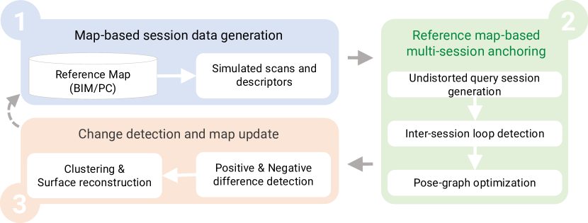
Figure 1: Overview of SLAM2REF. The pipeline consists of three steps: map-based session data generation, Reference map-based multi-session anchoring, and Change detection and map update.

4.1 Map-based session data generation (Map to Session Data)

In this step, our objective is to encapsulate the geometry of the reference 3D map—whether it is a BIM model or a point cloud—into individual LiDAR scans with their corresponding feature descriptors. These descriptors serve to encode the visible geometry from the origin of the scan within the reference map, enabling us to rapidly find the correct alignment of real-world session data with a reference map.

In real-world data acquisition, SD (SD) refers to consecutive sensor data acquired from a particular place at different periods [12]. Nonetheless, since we aim to convert a reference map to synthetic SD, these data can be considered a set of LiDAR scans (with known carefully selected positions) and their corresponding descriptors.

Formally, a session $\mathcal{S}$ is defined as follows:

$$\mathcal{S}:=\left(\mathcal{G},\left\{\left(\mathcal{P}_{i},d_{i}\right)\right\}_{i=1,\ldots,n}\right)$$ (3)

Here, $\mathcal{G}$ is a pose-graph map that contains the coordinates of the pose nodes, odometry edges, and optionally recognized intra-session loop edges with uncertainty matrices. These matrices represent how certain the positions of these edges are. This map can be saved in a text file, usually in .g2o format.

The $\left(\mathcal{P}_{i},d_{i}\right)$ are the pairs of 3D LiDAR scans with their corresponding global descriptors of the $i^{th}$ keyframe and $n$ is the total number of equidistantly sampled keyframes.

Generating synthetic SD (simulated scans and descriptors) from a reference map can be subdivided into three substeps. First, an OGM is extracted from the reference map. This extraction is achieved in an automated manner, taking as input only the IFC model or the reference point cloud and the floor level (z coordinate value) from where the OGM should be generated. In a second substep, the OGM is used to find the poses in which the LiDAR scans will be simulated. In a third and final substep, LiDAR scans are rapidly simulated in the positions calculated in the previous step, and the corresponding descriptors are calculated.

These substeps have been optimized so that it is possible to efficiently simulate data from large-scale 3D BIM models and point clouds. The following subsections provide a more detailed explanation of each substep.

4.1.1 OGM from reference map

Initially, and for convenience, the 3D geometry of the reference map is reduced into a 2D OGM. This dimensional reduction has been demonstrated to be very computationally efficient, allowing the implementation of the pipeline in complex, large-scale models.

Moreover, a 2D OGM (with known scale and origin) allows the direct usage of the map with the ROS navigation stack for autonomous navigation [59]. Besides path planning, cost maps, and navigational algorithms, the ROS navigation stack includes several state-of-the-art features, such as the regulated pure pursuit algorithm to adjust the robot’s speed depending on the path with a particular focus on safety in constrained and partially observable spaces [61].

The method for creating OGM varies based on the input data. Here, we outline how to do it for BIM models and point clouds.

OGM from IFC model (BIM2OGM)

The proposed automated generation of OGMs from BIM models builds upon prior work described in [78]. However, the key distinction lies in the enhanced automation of the pipeline.

For this purpose, we leverage the IfcConvert [33] tool and employ image-processing techniques akin to previous related works. IfcConvert, a command-line interface application within the open source IfcOpenShell project [46], facilitates the versatile conversion of a 3D BIM model from the .ifc file format to various other formats such as 3D meshes (.obj, .dae) or 2D layers (.svg). Detailed documentation for the IfcConvert functionality is available [34].

The input 3D IFC model is first converted to SVG format and then processed with the OpenCV library to output different layers as PNG files. These layers will then be merged to produce the final PGM.

To ensure compatibility with the ROS navigation stack and facilitate accurate scan simulations, the 2D PGM map must adhere to specific guidelines. It should represent unknown (external) regions in gray, navigable space (floor) in white, and potential collision-causing objects (e.g., walls and columns) in black.

IfcConvert is used to convert the 3D IFC model into 2D SVG files with the desired elements intersecting a plane at the chosen height. Furthermore, the resolution and size of the output SVG image are modified to only include the elements of interest.

To generate the OGM, we leveraged the semantics of the BIM model, focusing on extracting permanent elements like walls, ceilings, columns, and floors. This process excludes non-permanent features and objects invisible to LiDAR sensors, such as spaces, doors, windows, and curtain walls.

Filtering just permanent structural information about the building enables finding reliable correspondences between the geometry from the BIM model and real-world 3D LiDAR data. In this letter, we assume that the permanent structures in the BIM model are reliable features for localization and scan-matching. In the presence of open doors and windows, their exact placement in the space is unknown (open, closed, or semi-open) and is not provided in the BIM model; therefore, those elements should not be considered while creating the 2D OGM or any source of information used for alignment or localization.

A critical consideration in the conversion of SVG files to PNG format is the choice of units utilized within the original SVG file. By default, IfcConvert assigns millimeters as the unit of measurement for the SVG files. However, these millimeters do not undergo a direct one-to-one transformation to pixels during the conversion to PNG. Consequently, it becomes imperative to eliminate explicit unit specifications within the SVG file to ensure consistent scaling and preservation of the established coordinate origin during the conversion to PNG.

Additionally, it is critical to consider the effect of displacement while creating sections at different heights. While the scale will be maintained, the values of the coordinates of the geometry (saved in paths) in the SVG file will be adjusted according to the elements that intersect that specific height. To counteract this effect and have all the PNG images in the same coordinate system, the images are shifted according to the $x$ and $y$ values saved in the data matrix of the SVG generated with IfcConvert.

Automating the creation of the OGM involves producing the following two sections:

1. In the indoor layer, the floor area is designated as white. This section is generated at the z-coordinate corresponding to the upper surface of the slab of interest, i.e. at the floor level where the alignment should happen. Subsequently, the resultant gray-scale PNG image from this SVG is converted to binary. Then, its inverted version represents the indoor layer, in which the floor is represented as white pixels and the rest as black.

2. In the collision layer, we extract permanent elements like walls and columns while excluding non-permanent structures such as doors and windows. The creation of this layer occurs slightly above (1 m) the z-coordinate of the previous layers. It is crucial to note that the coordinate system of this image deviates from the preceding layer due to its creation at a different height. Therefore, it is imperative to compensate for this offset, as previously explained, before converting it into PNG format.

Subsequently, the indoor layer is placed over a gray image of the same size, allowing to distinguish outdoor (unknown) and indoor areas.

Finally, the pixels in the black color of the collision layer are transferred to the indoor layer. Given this, the final OGM is created and saved in the rasterized ROS standard PGM format. Figure 2 illustrates the layers and the final 2D map.

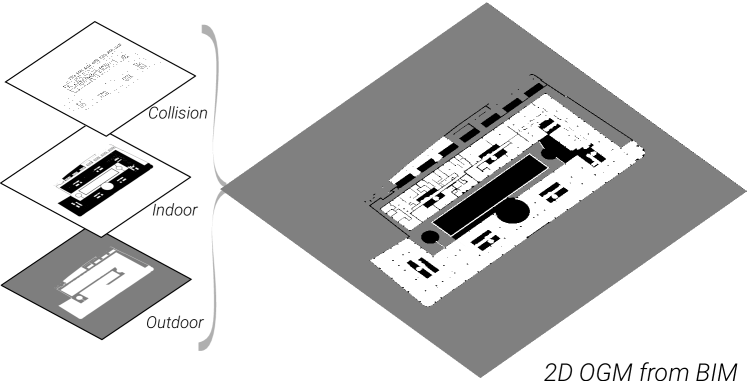
Figure 2: Generated OGM from the BIM model. On the left, the different layers, and on the right, the merged final OGM.

Additionally, a corresponding YAML configuration file is generated, containing crucial details such as the origin and resolution of the 2D map, extracted from the data-matrix of the initial SVG file.

Besides being an essential step in our pipeline, accurately creating a 2D OGM holds significant potential for SOTA localization algorithms, facilitating rapid and collision-free autonomous navigation. This has been exemplified by [78] and corroborated by numerous other studies (refer to Section 3).

OGM from a point cloud

The steps involved in creating a OGM from a point cloud are as follows: First, a 2D grid is created to the length and width of the point cloud and scaled given a grid resolution. Each cell within this grid is initially assigned a gray color.

Then, and as discussed in [80], the points are projected onto the XY plane, considering the resolution of the grid and its origin (the minimum XY coordinate of the point cloud). If points within a cell are found to be near the floor level (within a range of ±0.5 m), the cell is colored white, signifying navigable space.

On the other hand, cells are colored black if points are detected at a height 1 m above the floor level, assuming that this region predominantly consists of walls, columns, and other permanent elements.

4.1.2 Locations for data simulation

Once a correct OGM is generated from the reference map, this is utilized to find proper locations where LiDAR scans will be simulated. These locations should be equally separated coordinates ordered by proximity, aiming to closely replicate real-world data acquisition with full coverage of the map. To this aim, we first extract the skeleton of the image, which gives a smooth path similar to the one a person would follow during acquisition with a mobile LiDAR or scanning device. Then, points are sampled over this path in a uniform manner.

Similarly, as proposed in [78], the process extracts a skeleton from the OGM. This skeleton is derived using the approach outlined by [52], producing a smooth trajectory over the free space that interconnects all rooms and open areas within the OGM.

In a previous version of our pipeline [79], we used a Wavefront Coverage PP [88] over this skeleton to find the waypoints in which the 3D LiDAR will be simulated. However, the Wavefront Coverage PP approach is inherently intricate, making it unfeasible to be applied over large OGMs without consuming large amounts of computational resources.

Therefore, to handle large-scale reference maps, we propose the following method instead, which tries to sample uniformly key points over the path created with the skeleton approach:

(1) The scan locations are initially extracted using image processing techniques. This involves generating masks with equally spaced vertical and horizontal lines, isolating only the white pixels intersecting these masks and the previously generated skeleton. The idea behind this is that only isolated pixels will remain rather than elongated lines present in the skeleton.

(2) Subsequently, the corresponding center points of the remaining pixels are extracted using a contour detection algorithm. To ensure a minimum distance between points, the spatial distribution of these coordinates is downsampled.

(3) Finally, the coordinates are sequentially ordered using the nearest neighbor algorithm.

Figure 3 shows the calculated scan locations for an OGM of a large building.

Figure 3: Calculated locations for scan simulation. On the left are the main steps, and on the right are all the calculated positions in the entire OGM.

4.1.3 LiDAR data simulation

In our previous work [79], we utilized the identified waypoints to set navigational goals for a robot operating autonomously within the ROS navigation stack, simulated in the Gazebo physics engine [38]. Then, a sequence of simulated 3D LiDAR scans was produced with Gazebo and saved in rosbag files. Here, we present an enhanced approach that eliminates the need for ROS or Gazebo; by such means, we avoid the creation of large rosbag files containing redundant information.

Instead, we propose leveraging BlenSor, a versatile software designed for simulating various range scanners [24, 27]. With the BlenSor API, we can automatically load the coordinates for simulating LiDAR scans (calculated in the previous step), streamlining the simulation process.

The process of simulating LiDAR data can be subdivided into three main steps:

1. The reference map is converted to an STL mesh. In the case of a BIM model, this involves conversion to OBJ format after filtering only permanent structures using IfcConvert, similar to the process employed in creating the 2D OGM. However, instead of generating an SVG file, our method creates an OBJ file containing the 3D geometry of the model described explicitly. To ensure precise 3D conversion, our approach selectively includes required permanent elements (e.g., walls, columns, floors, and slabs) rather than excluding entities. Our experiments revealed that the exclusion command does not consistently produce satisfactory results for this 3D conversion. Subsequently, the generated OBJ file is converted to STL format for seamless integration of the geometry into BlenSor.

   When dealing with a point cloud as the reference map, the ball pivoting method has consistently demonstrated reliability in reconstructing mesh surfaces from 3D point clouds. Before applying this method, the process involves estimating the normals of the point cloud and calculating an optimal radius based on the average nearest neighbor distance, facilitating accurate and efficient surface reconstruction.

2. Later, the coordinates determined in the preceding steps, where the data will be simulated, are transformed from pixels (in 2D) to meters (in 3D). This conversion utilizes the scale and origin information specified in the YAML file of the corresponding OGM.

3. Subsequently, the simulated LiDAR properties are adjusted to align with those employed in real-world scanning. Then, a sub-process initiates the parallel simulation of $360^{\circ}$ LiDAR scans at these coordinates using BlenSor.

Finally, and after the simulation, SC descriptors are created for each simulated scan. More information about these descriptors will be provided in the following section 4.2.1 (Step 2.1).

Following the steps above, the geometry of the reference map or the permanent objects in the BIM model is now established as a reference session, denoted as $\mathcal{S_{R}}$, and is illustrated in Figure 4.

In the subsequent step, this synthetic SD, encompassing descriptors and simulated scans, will be leveraged for fast place recognition and data alignment. However, before this process, it is necessary to generate session data from real-world datasets.

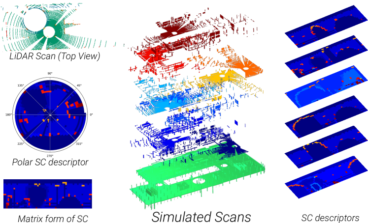
Figure 4: Synthetic session data from the reference map. On the left, from top to bottom: Top view of one LiDAR scan, its corresponding polar scan context (SC) descriptor, and the descriptor in the matrix form. In the middle, a set of simulated scans and the STL mesh from the BIM model are used. Right, corresponding SC descriptors for the simulated scans.

4.2 Reference map-based multi-session anchoring

To derive a globally consistent map aligned with the reference map from real-world sequential LiDAR data, the following three substeps are executed: (1) Creation of the real-world motion-undistorted query session $\mathcal{S_{Q}}$, which is similar to the synthetic reference session $\mathcal{S_{R}}$ (created as explained in the previous section); however, from real-world data. (2) Place recognition for inter-session loop detection between $\mathcal{S_{Q}}$ and $\mathcal{S_{R}}$. (3) Pose graph optimization with multi-session anchoring and pose refinement with KNN loops and a final ICP registration. These substeps are described in detail in the following subsections.

Figure 5 illustrates a flowchart outlining the complex multi-session anchoring process in the SLAM2REF framework.

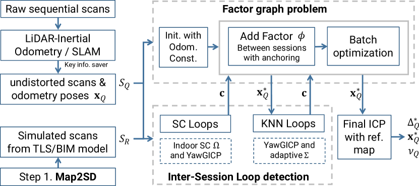
Figure 5: Comprehensive flowchart illustrating the multi-session anchoring process within SLAM2REF. This process includes the generation of session data from the reference map $\mathcal{S_{R}}$, creation of the real-world query session $\mathcal{S_{Q}}$, inter-session loop detection using Indoor Scan Context and YawGICP, and pose refinement with KNN loops and final ICP. The outcome includes the anchor node $\Delta_{Q}^{*}$, optimized 6-DoF poses $\textbf{x}_{Q}^{*}$, and a confidence level list $\mathbf{\nu}_{Q}$ for each pose in the query session.

Following the generation of session data (SD) from the reference map $\mathcal{S_{R}}$ (Step 1 presented in Section 4.1) and the construction of the real-world query session $\mathcal{S_{Q}}$ (Section 4.2.1), the alignment procedure can be initiated. This involves an inter-session loop detection phase employing Indoor Scan Context and YawGICP (Section 4.2.2), which identifies encounters $\mathbf{c}$ denoting correspondences between the sessions. These encounters, along with initial odometry constraints, are integrated into a factor graph problem. Subsequent to optimization, pose refinement is carried out using KNN loops (Section 4.2.3) and a final ICP process. The resulting information comprehends the following elements attributed to the query session: the anchor node $\Delta_{Q}^{*}$, which facilitates the global alignment to the reference map, the optimized 6-DoF poses of each scan $\textbf{x}_{Q}^{*}$, and a confidence level list $\mathbf{\nu}_{Q}$ providing the reliability of each pose after scan registration.

4.2.1 Creation of the real-world query session

The correct generation of a query session $\mathcal{S_{Q}}$ from real-world data involves three primary substeps, elaborated upon as follows.

Motion distortion correction Point clouds acquired from mobile spinning LiDAR sensors often experience motion distortion because the rotating laser array collects points in various instances during a sweep, leading to inaccuracies. Therefore, one of the main issues using LiDAR-only algorithms is the difficulty in correcting motion-distorted LiDAR scans in the presence of fast motion.

In some SOTA LiDAR-only SLAM algorithms, the authors have assumed constant velocity models to overcome this issue, as done in KISS-ICP [77]. Although this assumption can hold for data acquired with LiDAR placed over autonomous cars and simplistic motion patterns, as in the KITTI raw dataset [25], the constant-velocity model cannot capture subtle movements and generally does not hold for data acquired with handheld devices or Unmanned Vehicles (UVs) in indoor or outdoor scenarios [90].

Therefore, we take advantage of the MDC of one SOTA LIO system to generate undistorted scans before alignment with the reference map.

In particular, we leverage the MDC implementation in DLIO [14], which, inspired by [21], generates continuous-time trajectories. Their approach considers a motion model characterized by constant jerk and angular acceleration compensated with IMU measurements. This enables fast and parallelizable point-wise motion correction.

Once the scans are deskewed with the information from the IMU, keyframe scans can be extracted with timestamps and odometry calculated poses. This process is explained in the subsequent section.

Key information saver The goal here is to save equally spaced undistorted scans (i.e., after a specific variation of time, translation, or rotation) with respective odometry estimated poses from a sequence of data that was previously recorded in a ROS bagfile during acquisition with a mobile mapping system device.

To extract keyframes and construct the real-world query session $\mathcal{S_{Q}}$, the methodology proposed by [48] presents a viable approach. The authors implemented loop closure mechanisms and keyframe information-saving capabilities as an extension in several SOTA algorithms.

In general, the approach can vary depending on the available data. When dealing with LiDAR-only data, SC-A-LOAM [48], an enhanced version of A-LOAM [89] is a valid technique; however, it assumes constant velocity for MDC. For an additional calibrated 9-axis IMU, the corresponding enhanced version of LIO-SAM [71] can be used.

If we deal with 9-axis or only 6-axis IMU measurements, which are typical for the internal IMUs of LiDAR and camera sensors, our open source keyframe information saver together with almost any LIO pipeline can be used (e.g., FAST-LIO2 [82], FASTER-LIO [11] or iG-LIO [15]). Something essential to consider is that the LIO pipeline should publish (i.e., make available) the ROS topic with the undistorted scan in the local coordinate system. This last characteristic is not standard and depends on the used MDC strategy.

Since DLIO showed the best MDC results in our experiments, we implemented and made open-source the corresponding enhanced version that transforms the deskew scan to the correct local pose after undistortion.

After saving the keyframe scans along with odometry information (i.e., time-stamped approximate 6-DoF poses), the final step to generate the query session involves feature descriptor extraction to encode the geometric information of the scans. This process will facilitate efficient comparison with reference session descriptors later.

Indoor Scan Context descriptor For place recognition, we introduce the new ISCD. This variant diverges from the original Scan Context descriptor by focusing exclusively on indoor scans, as opposed to outdoor scans typically encountered in autonomous car environments, for which SC was originally conceived. With ISCD, our objective expands beyond merely eliminating ceiling points, which are notably common in indoor scans, especially in acquisitions with significant variations in pitch and roll angles, as usually encountered in handheld systems. Moreover, we aim to selectively filter permanent vertical building elements perpendicular to the XY-plane, characterized by visible vertical surfaces of considerable length.

Inspired by [40, 37], and by the formal definitions in [81, 53], the creation of ISCD is as follows: Azimuthal and radial bins split the 3D scan from the top view following an equally spaced arrangement (for reference, see an example on the left side of Figure 4).

In the Cartesian coordinate system, we defined a LiDAR scan with $n$ points as $\mathcal{P}=\left\{\mathbf{p}_{1},\mathbf{p}_{2},\cdots,\mathbf{p}_{n}\right\}$ with each point $\mathbf{p}_{\mathbf{k}}=\left[x_{k},y_{k},z_{k}\right]$. Each point $p_{k}$ can be converted into a polar coordinate system, as follows:

$$\mathbf{p}_{\mathbf{k}} =\left[r_{k},\theta_{k},z_{k}\right],$$

$$\ r_{k} =\sqrt{x_{k}^{2}+y_{k}^{2}},$$

$$\theta_{k} =\arctan\frac{y_{k}}{x_{k}}.$$

The point cloud is then segmented into $N_{s}$ sectors and $N_{r}$ rings by equally diving polar coordinates in azimuthal and radial directions. Each block is represented by:

$$B_{ij}= \left\{\mathbf{p}_{\mathbf{k}}\in\mathcal{P}\mid\frac{(i-1)\cdot R_{\max}}{N_{r}}\leq r_{k}<\frac{i\cdot R_{\max}}{N_{r}},\right.$$

$$\left.\frac{(j-1)\cdot 2\pi}{N_{s}}-\pi\leq\theta_{k}<\frac{j\cdot 2\pi}{N_{s}}-\pi\right\},$$

where $i\in\left[1,N_{s}\right],j\in\left[1,N_{r}\right]$, and $R_{\max}$ is the maximum radius considered to create the descriptor. In contrast with the original SCD, instead of taking only the $z$ value of the highest point in the bin $b_{ij}$, in ISCD, we only assign a value equal to 1 if there are a minimum of $ISC_{\text{min}}$ points in the bin, and 0 otherwise. Formally:

$$b_{ij}=\begin{cases}1&\text{if }\text{count}(\mathbf{p}_{\mathbf{k}}\in B_{ij})\geq ISC_{\text{min}}\\ 0&\text{otherwise}\end{cases}$$

The final ISCD $\Omega\in\mathbb{R}^{N_{r}\times N_{s}}$, can be generated by:

$$\Omega(i,j)=b_{ij}.$$

The global signature $\Omega$ is a $2\mathrm{D}$ matrix that efficiently encodes the geometry of mainly permanent elements (e.g., walls and columns) visible from the position of the sensor.

Note that if $B_{ij}\in\varnothing$, $\Omega(i,j)=b_{ij}=0$, i.e., if in the bin there are no scan data because the bin is free or occluded, the bin will have a value of zero and will be visible as a blue color in the image representation of the descriptor (as shown in 4 and 6).

In the following section, these descriptors are exploited to rapidly determine the rough alignment between the query and reference sessions.

4.2.2 Place recognition for inter-session loop detection

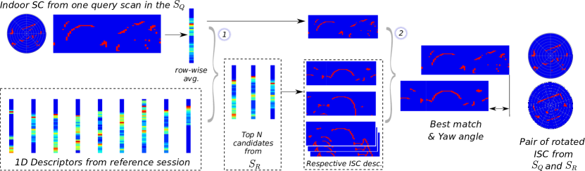
Figure 6: Indoor Scan Context loop detection: The query session’s scan is converted into 1D rotational invariant descriptors. These descriptors are quickly compared with those from the reference session to select the top $N_{c}$ candidates (see number 1). In the second phase, the 2D descriptors of these candidates are compared using cosine similarity while systematically varying the column position to identify the best match and optimal yaw angle alignment.

Having $\mathcal{S_{Q}}$ (real-world query session) and $\mathcal{S_{R}}$ (session from the reference map), we aim to align these two sessions. With this aim, we look for correspondences comparing the previously generated ISCDs between the sessions to find inter-session loop closures. This task is also known as place recognition, in which one aims to identify or determine the specific location or place of sensor measurements (in our case, single LiDAR scans) within a given map.

In order to facilitate quick comparison, the 2D descriptor is condensed into a one-dimensional vector. This vector is generated by calculating the average of the rows in the 2D descriptor. This average ensures rotation invariance, meaning that if a scan is in a location that is approximately the same but with a different yaw angle, the resulting 1D descriptor will remain unchanged.

The comparison between the query scan (from $\mathcal{S_{Q}}$) and the scans from the $\mathcal{S_{R}}$ is facilitated by employing a KNN search in a KD-Tree and using the L2-norm metric.

Subsequently, the corresponding 2D descriptors of the $N_{c}$ closest 1D descriptors are compared using the column-wise cosine distance.

This column-wise cosine distance is calculated to identify the similarity between two ISCDs $\Omega^{q}$ and $\Omega^{r}$. Let $\mathbf{v}_{i}^{q}$ and $\mathbf{v}_{i}^{r}$ be the $i^{th}$ column of $\Omega^{q}$ and $\Omega^{r}$; the score can be found by:

$$\varphi_{i}\left(\Omega^{q},\Omega^{r}\right)=\frac{1}{N_{s}}\sum_{i=0}^{N_{s}-1}\left(\frac{\mathbf{v}_{i}^{q}\cdot\mathbf{v}_{i}^{r}}{\left\|\mathbf{v}_{i}^{q}\right\|\cdot\left\|\mathbf{v}_{i}^{r}\right\|}\right).$$

A comparison conducted column by column is beneficial for handling dynamic entities or slight differences between the reference map and the query session (e.g., new furniture or clutter) since although some columns of the 2D descriptor may show variations, the remaining columns will exhibit similarities. However, relying solely on this comparison overlooks the possibility of revisiting the exact location from a different perspective. To tackle this limitation and ensure rotational invariance in the matching process, the method computes distances using a range of column-shifted scan contexts. Then, it identifies the shift that yields the minimum distance. This procedure resembles the coarse alignment of two sets of points, focusing mainly on aligning the yaw angle. By implementing this approach, the optimal number of column shifts (i.e., optimal yaw angle) for alignment and the corresponding minimum distance can be determined.

Formally, if we compare $\Omega_{k}^{q}$ and $\Omega^{r}$ where $\Omega_{k}^{q}$ is $\Omega^{q}$ shifted by $k^{th}$ column. The final score is calculated as follows:

$$\Phi_{i}\left(\Omega^{q},\Omega^{r}\right)=\underset{k}{\operatorname{argmin}}\ \varphi_{i}\left(\Omega_{k}^{q},\Omega^{r}\right).$$

The matched pairs are subsequently refined through a filtering process employing an empirical threshold, denoted as $\epsilon$, applied to the calculated minimum distance metric, $\Phi_{i}$.

After detection of ISC loop closures, a 6D relative constraint is established between two keyframes if there is a successful alignment between a sub-map from the reference session, denoted as $\mathcal{P}_{R,i}$ (which comprises the three closest scans to the one that matched the scan in the query session), and the single undistorted scan from the query session, denoted as $\mathcal{P}_{Q,j}$.

The correctness of the alignment between these two keyframes is essential for the subsequent steps in the pipeline, as it dictates the effectiveness of the initial global registration between sessions.

To achieve this alignment in a robust way, we introduce YawGICP, an improved variant of the GICP algorithm. YawGICP primarily focuses on translational changes and yaw angle adjustments, thereby mitigating significant pitch or roll rotations commonly induced by conventional GICP alignment procedures. This precaution prevents instances where standard GICP may accidentally rotate the source point cloud by 90 degrees (in pitch or roll), leading to erroneous associations between wall, ceiling, or floor points.

The YawGICP is initialized with the yaw angle calculated in the previous step.

Consistent with prior work [79, 41], only ISC loops exhibiting a satisfactory fitness score, indicating a high percentage of inliers, are considered. These loops are then incorporated into the factor graph problem with low covariance $\Sigma_{c}$, serving as factors between sessions with anchoring. Further elaboration on the factor graph problem will be provided in the subsequent section (4.2.3). Figure 7 illustrates the detected ISC loop closures, which are then classified into correct and incorrect using YawGICP.

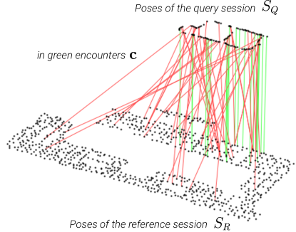
Figure 7: Detection of Indoor Scan Context loop closure between sessions. On the top are the poses from the query session, and on the bottom are the poses from the reference session, in this case, created from a BIM model. Correct correspondences are represented by green lines, while erroneous ones as red. After the YawGICP step, the erroneous correspondences are effectively discarded.

4.2.3 Pose graph optimization and data alignment

In this substep, the initial odometry constraints derived from the preserved session data (referenced in substep 4.2.1) and previously identified inter-session ISC loop closures (introduced in substep 4.2.2) are leveraged to achieve the data alignment.

The objective is to first roughly align the entire query session with the reference session from the reference map. Consequently, even if some scans within the query session’s keyframes do not have any correspondence with the reference session, they are still aligned to the most cohesive pose based on the identified correspondences (SC loops) with adjacent scans and the provided odometry constraints.

Formally, in this contribution, the alignment between the sessions is done using multi-session anchoring. This method was originally introduced by [42] and was further developed by [57], [63], [41]. One of the main motivations behind these projects is to solve the so-called multi-robot mapping problem. In this context, and as explained in Section 2, maps generated by different robots commonly have distinct reference coordinate systems, which require the merging of these maps to form a globally consistent map with a unified global coordinate system.

We formally define our problem as follows: Given two sessions, $\mathcal{S_{Q}}$ and $\mathcal{S_{R}}$, each provided with odometry constraints, and in the case of $\mathcal{S_{Q}}$, potentially equipped with intra-session loop closure constraints identified by a SLAM algorithm with a key information saver (as explained in Section 4.2.1), our objective is to determine the optimal poses for the nodes in $\mathcal{S_{Q}}$. These poses should effectively align the measurements within $\mathcal{S_{Q}}$ with those of $\mathcal{S_{R}}$, considering the existence of inter-session loop closure constraints between the two sessions.

As explained in 2, multi-session anchoring can be formulated as a factor graph MAP optimization problem.

To properly consider the encounter measurements ($\mathbf{c}$) in the MAP formulation in Eq. (2), we need to redefine the relative measurement model $h{\big{(}}.{\big{)}}$ in the global frame with the help of the anchor nodes.

This adjustment is needed, considering that the encounter is a global assessment between two trajectories. However, the pose variables for each trajectory are defined in the session’s local coordinate frame. With the anchor nodes, the poses of the respective sessions are transformed into a global frame, where a comparison with the measurement becomes possible.

The measurement model $h{\big{(}}.{\big{)}}$ is modified to $h^{\prime}{\big{(}}.{\big{)}}$, to incorporate the anchor nodes, and therefore, the respective term in Eq. (2) is changed to:

$$\sum_{j\in N_{e}}\left\|h_{j}^{\prime}\left(\mathbf{x}_{R,j},\mathbf{x}_{Q,j},\Delta_{Q},\Delta_{R}\right)-\mathbf{c}_{j}\right\|_{\Sigma_{c}}^{2}$$

The difference $\mathbf{c}$ in the global frame between a pose $\mathbf{x}_{R}$ and a pose $\mathbf{x}_{Q}$ is estimated by $\mathbf{c}=\left(\Delta_{R}\oplus\mathbf{x}_{R}\right)\ominus\left(\Delta_{Q}\oplus\mathbf{x}_{Q}\right)$, where $\oplus$ and $\ominus$ are the $\mathrm{SE}(3)$ pose composition operators [73, 5].

The operation $\Delta_{Q}\oplus\mathbf{x}_{Q}$ represents concatenating the transformation of $\mathbf{x}_{Q}$ (the second pose) to the reference system already transformed by the anchor node $\Delta_{Q}$. In $\mathrm{SE}(3)$, the operator $\oplus$ is equivalent to matrix multiplication [5].

Hence, the subsequent factor between sessions with anchoring will properly integrate the encounters in the pose graph optimization. It achieves this by initially transforming the poses of each session into the global frame using the anchor nodes.

$$\phi\left(\mathbf{x}_{R,i},\mathbf{x}_{Q,j},\Delta_{R},\Delta_{Q}\right)$$ (4)

$$\propto\exp\left(-\frac{1}{2}\left\|\left(\left(\Delta_{R}\oplus\mathbf{x}_{R,i}\right)\ominus\left(\Delta_{Q}\oplus\mathbf{x}_{Q,j}\right)\right)-\mathbf{c}\right\|_{\Sigma_{c}}^{2}\right)$$

While initializing the factor graph, the odometry constraints from both sessions and the constraints after ISC loop detection are added to the optimization problem, the first as between factors and the latter as factors between sessions with anchoring.

Considering that in our scenario, our objective is to use the coordinate system of $\mathcal{S_{R}}$ as the global system for alignment, the anchor node $\Delta_{R}$ of the reference session should be assigned an insignificantly small covariance ($\Sigma_{P}$). Conversely, for the anchor node $\Delta_{Q}$ of the query session, a significant covariance is assigned ($\Sigma_{L}$).

Moreover, the odometry poses are also added to the factor graph. However, since $\mathcal{S_{R}}$ comes from the reference map, its poses $\mathbf{x}_{R}$ are treated as fixed and should not be altered by the optimization. To avoid changes to these poses, they are added to the factor graph optimization problem as prior factors with very low covariance ($\Sigma_{P}$) in its noise model.

Following batch optimization, the intermediate optimized values of the anchor node $\Delta_{Q}^{*}$ and the poses $\textbf{x}_{Q}^{*}$ are obtained. However, these poses are expressed in the local coordinate system of $\mathcal{S_{Q}}$. To convert them from this local coordinate system (denoted as ${}^{Q}\mathcal{G}_{Q}^{*}$) to the global coordinate system ${}^{W}\mathcal{G}_{Q}^{*}$ of the reference map, we apply the following transformation to each pose $\mathbf{x}$ in the graph:

$${}^{W}\mathbf{x}_{Q}^{*}=\Delta_{Q}^{*}\oplus{}^{Q}\mathbf{x}_{Q}^{*},$$

where $W$ is the global coordinate system, or in our case, the coordinate system of the reference session.

After the previous step, the query session roughly aligns with the reference session. To further refine the poses of the query session, we introduce a rapid KNN loop detection method with adaptive covariance. Initially, submaps are generated by selecting KNN scans from the scan to be aligned within the query session, along with the k-nearest scans from the reference session. Subsequently, the YawGICP algorithm (see 4.2.2) is employed to register these two submaps, and the quality of registration is assessed based on a predefined fitness threshold, classifying the alignment as either good, acceptable, or unacceptable.

Upon acceptance of the alignment, the constraints are added to the optimization problem as factors between sessions with anchoring with adaptive covariance. This adaptive covariance strategy assigns a very low covariance in the noise model to constraints originating from well-registered keyframe submaps, while constraints from just acceptable registrations receive a higher covariance. This approach allows the pose graph optimization to appropriately weigh the influence of these constraints in calculating optimized poses.

After conducting batch optimization one more time with incorporated odometry, ISC, and KNN constraints in the factor graph problem, the resulting poses undergo further refinement through a final ICP registration. Unlike previous steps that relied on registration with simulated scans from the reference map, this stage utilizes a one-centimeter-dense point cloud obtained from the reference map as the registration target. In case the reference map is a BIM model, this point cloud is created by sampling uniformly points over a mesh of permanent elements in the building (i.e. without doors and windows similarly as done in Step 1, section 4.1.1)

Due to the high density of the target point cloud, GICP fails to offer any significant advantage over P2P-ICP [6]. In fact, in specific scenarios, GICP yields inferior results. Therefore, we have opted to use P2P-ICP, which not only produces competitive results but also operates considerably faster.

To speed up computations and avoid the time-intensive KNN search associated with registrations involving a large target point cloud, scans within the query session are allocated into proximity-based groups. Subsequently, for each group, a target point cloud is created, dynamically cropping the reference map into spheres. The individual source scans within each group are then registered concurrently, leveraging parallel computing techniques.

The registration results are evaluated using three metrics. One metric is the RMSE, and the other two correspond to fitness scores calculated at two distinct maximum P2P distances: $F_{1}$ and $F_{2}$. The fitness score is the percentage of source inliers, considering a maximum P2P distance threshold to classify points as inliers after registration.

These metrics are computed explicitly for points located within 30 cm from the target point cloud after registration. This approach ensures the exclusion of points outside the reference map or those influenced by significant environmental changes, such as the addition of new walls or large pieces of furniture.

Depending on the metric values, the resulting aligned scans are categorized into four classes: Perfect, Good, Bad, and Outside the Map. The result is saved on a list, denoted as $\nu_{Q}$.

The resulting poses will be used in the subsequent step to create the final aligned map and compare it accordingly with the reference map.

4.3 Change detection and map update

Following the completion of the prior steps, the two sessions have been precisely aligned, and they now share a unified coordinate system. Subsequently, a comprehensive 3D map of the most up-to-date environmental state can be generated by placing the keyframes $\mathcal{P}_{Q,i}$ from the query session $\mathcal{S_{Q}}$ in the estimated poses ${}^{W}\mathbf{x}_{Q,i}^{*}$, which are now in the global coordinate system.

If desired and to ensure the integrity and fidelity of the final map representation, it is recommended to exclusively incorporate scans classified as ”perfectly” or ”good” aligned within $\nu_{Q}$ during the map construction process.

However, it is essential to note that although the remaining poses may not meet the strict alignment criteria with the reference map, they have already undergone significant optimization through odometry and loop closure constraints. Consequently, they can be utilized to generate the final map and even extend the reference map if the scan extends beyond its boundaries.

Since both maps are now aligned, a comparison of the two 3D maps becomes feasible. The comparison process involves categorizing the elements in the map into three distinct types: Positive differences (PDs) denote instances where new objects have been introduced compared to the reference map; negative differences (NDs) signify the removal of objects previously documented in the reference map; and unaltered elements (UEs) denote features that remain constant across both maps.

This categorization is facilitated with the OctoMap library [31]. OctoMap, a widely-used library in robotics and 3D mapping, operates by dynamically updating voxel occupancy status within its octree structure as new point clouds are integrated. The analysis of measurement densities in OctoMap enables us to distinguish between occupied and free space, facilitating reliable 3D mapping.

Additionally, we also leverage the probabilistic capabilities of OctoMap during measurement accumulation to facilitate the automatic removal of dynamic elements from the final point cloud. This removal is done based on occupancy patterns across multiple scans. The resulting map is the one used to detect PDs and UEs in the preceding step. Moreover, OctoMap calculates free space by identifying regions where the sensor fails to detect objects; this free space will be leveraged for NDs detection later.

To detect PDs and UEs, a P2P distance threshold is used between a point cloud from the reference map (also used in the previous final ICP step) and the newly created map with OctoMap, similar to what was presented in [79]. A signed distance computation allows the distinction of points that are near and far from the reference map. Near points allow for the confirmation of UEs, whereas distant points are regarded as PDs.

The point cloud of identified PDs is passed through an outlier removal process. Subsequently, the point cloud undergoes a segmentation process through the density-based clustering technique (DBSCAN). This step is based on a neighbor-distance threshold and a minimum number of points per cluster.

Lastly, for each PD cluster, a mesh is created using cubes from a VG of the point cloud.

Voxels, in contrast to other surface reconstruction approaches, capture the actual geometry of objects present in the scene. This leads to improved visualization of the new elements in conjunction with the reference map, providing a better understanding of the scene.

The process of detecting NDs involves conducting a visibility analysis using individual scans from the query session ($\mathcal{P}_{Q,i}$). As mentioned before, the OctoMap library facilitates this analysis by calculating the free space, i.e. areas where the LiDAR did not detect any objects from its origin point. Similarly, as with the PDs, this free space is used together with a P2P distance threshold against a point cloud sampled from the reference map to identify the NDs.

The regions at the intersection between the reference map and the free space are the NDs. These are then passed through the outlier removal and clustering process, removing isolated points and small clusters.

The final voxels are transformed into meshes and are colored blue for PDs and red for NDs. An exemplary result is depicted in 8.

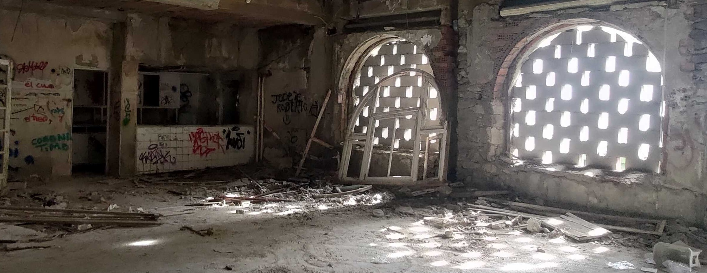
(a)

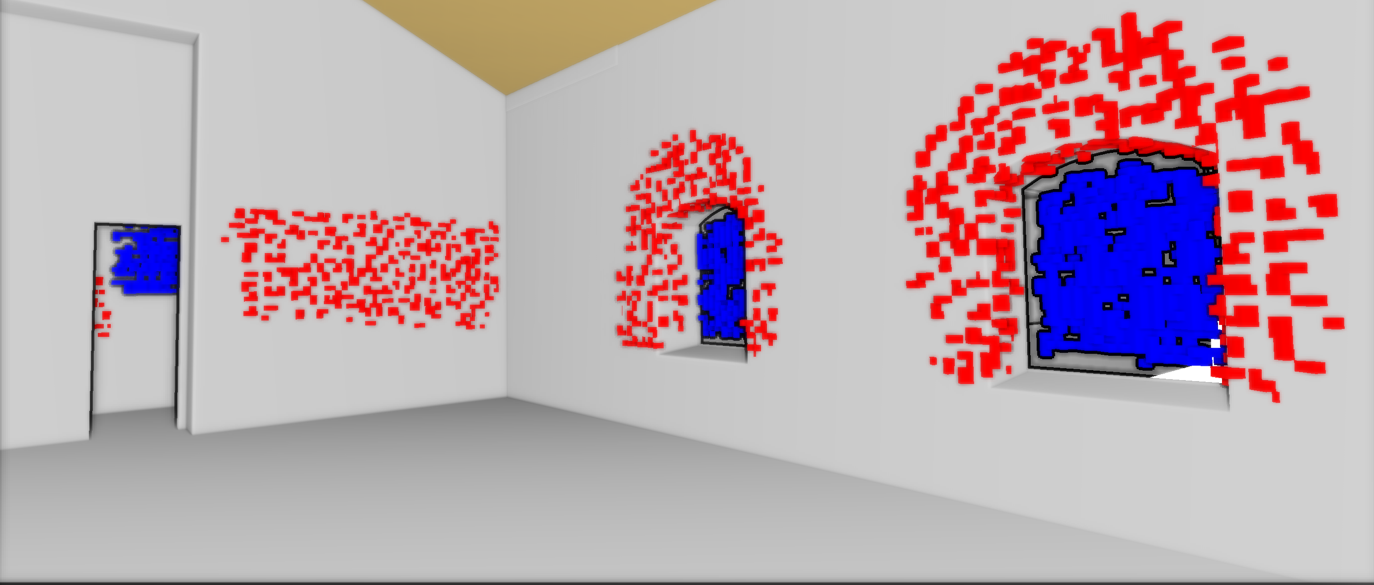
(b)

Figure 8: Positive and negative differences between the point cloud and the reference BIM model are illustrated as follows: (a) A picture of the real-world scene. (b) Visualization of the detected changes in the form of voxelized clustered meshes with positive differences depicted in blue and negative differences in red. Particularly, it is visible that the windows in the model are smaller compared to the real-world windows.

5 Experiments

In this section, we present the data used to evaluate the efficacy of the proposed strategies. Comprehensive implementation details, such as the values of the essential parameters, are meticulously outlined to ensure a thorough understanding of our approach.

5.1 ConSLAM dataset

To ensure reproducibility and benchmarking, we evaluated our approach by applying it to the recently released open-access ConSLAM dataset [75, 74].

The ConSLAM dataset consists of four sequences of a construction site captured with a handheld system. It incorporates synchronized timestamped LiDAR scans, 9-axis IMU measurements, and RGB and NIR camera images.

Given the TLS point cloud of sequence number two, we elaborate a half-centimeter-accurate BIM model.

We used the OA-LICalib library [54, 55] to retrieve the extrinsic calibration parameters (rotation and translation) between the LiDAR and the IMU sensors.

5.2 Implementation details

While Step 1 and 3 were implemented in Python, Step 2 was written in C++.

5.2.1 Step 1: Reference session generation

In Step 1, to generate the reference session data ($\mathcal{S_{R}}$), the vertical FoV of the simulated LiDAR scans can be customized according to preferences. To achieve alignment with a TLS point cloud as a reference map, the simulated LiDAR scans encompass a range from -45 degrees to 45 degrees in the vertical FoV. However, in our experiments, while aligning the data with a BIM model, we observed improved ISC loop detection when no ceiling points were present in the simulated scans. Consequently, the scans are adjusted to cover only from 0 to -25 degrees in the vertical direction. In Blensor, during the LiDAR simulation process, the noise was set to a mean of zero with a standard deviation of 0.03 m, an angular resolution of 0.1728 degrees, and a maximum distance of 15 m.

5.2.2 Step 2: Query session generation, alignment, and correction

Step 2.1: Query session creation In Step 2, to generate the query session from the real-word data ($\mathcal{S_{Q}}$), for the MDC step, we opted for using DLIO, because, in contrast to FAST-LIO2 [82], it does not require heavy downsampling of the point cloud for deskewing and registration. Hence, clean, undistorted scans with DLIO allow dense map reconstruction. As suggested by [85], we reproduced the data in the bagfiles at a low rate (half of the original speed) to avoid errors during the distortion process. Regarding the key information saver, while it is possible to await a minimum variation on translation or rotation between consecutive scans, we opted to save scans given either a list of timestamps or after a specific interval of time has passed. This feature is convenient since we want to compare our results with existing ConSLAM GT poses. Therefore, we are mainly interested in specific frames with known timestamps. For the creation of ISCD we opted for $N_{s}=60$, $N_{r}=20$ (as suggested in [37]), $ISC_{\text{min}}=40$, and a maximum radius of $10\text{\,}\mathrm{m}$.

Step 2.2: Inter-session loop detection with ISC Nanoflann [8] is used to create a KD-tree of 1D rotational invariant descriptors. A total of 100 ($N_{c}$) top candidates were chosen to evaluate in 2D after the 1D descriptor comparison; it is worth mentioning that the retrieval of correct correspondences is very sensitive to this value. A cosine similarity threshold $\epsilon=0.3$ is used to filter out pairs of 2D descriptors that passed with the minimum distance among the possible column shifts $k$. Only column shifts of 10% of the total number of columns (i.e., 36 deg) are considered for the alignment. All YawGICP registrations in the ISC and KNN loops are done using parallel computations with OpenMP. Unlike conventional ICP implementations, when employing YawGICP, it is imperative to express the target point cloud (i.e., from the reference map) in the local coordinate system of the source scan (i.e., the point cloud to be aligned). Otherwise, the process will yield undesirable results. This shift is critical because the resulting transformation matrix is relative to the origin of the source scan, with the aim of rotating the point cloud from its local origin rather than the origin of the global coordinate system.

Step 2.2: KNN loops, pose-graph optimization and final ICP

The KNN used to create the submaps for KNN loop detection in the second step of optimization is 5. To ensure correct alignment with the BIM model as the reference map, we opted to omit the KNN loop detection process. This decision was made because this process tends to induce erroneous correspondences. Meanwhile, in Step 2.3.2 (Section 4.2.3), the pose-graph optimization is done with GTSAM using iSAM2; the following are the values of the variances of the different noise models: $\Sigma_{L}=\pi^{2}$ (significant noise for query session’s anchor node); $\Sigma_{P}=1\times 10^{-102}$ (prior noise for reference map poses and initial poses); $\Sigma_{O}=1\times 10^{-4}$ (for odometry constraints); $\Sigma_{c}=0.5$ (robust noise for encounters, i.e., loop closure constraints). The parallel creation of spheres for target point cloud registration and the P2P ICP of the single source scans is done using OpenMP in C++. In our case, we use the following two maximum distances to calculate the fitness scores: $F_{1}=1$ cm and $F_{2}=3$ cm.

5.2.3 Step 3: Change detection and map update

In Step 3, the process is performed with Trimesh, OctoMap, and Open3D.

We use a P2P distance threshold of 0.3 m to calculate the positive and negative differences.

OGM2PGBM [78], Scan Context [40], and LT-SLAM [41] were projects that we used as a reference and that are freely available online.

For the evaluation of the results, presented in the following section, the trajectories were compared against the ground truth using evo [26] in TUM format [70] and using the Umeyama alignment [76].

6 Results and analysis

In this section, we provide the results of our pipeline with respect to the alignment with an accurate TLS point cloud and with a BIM model as a reference map.

Table 1 shows the APE summary of the different methods in each sequence of the ConSLAM dataset after alignment with the corresponding TLS point clouds. In the table, the performance of DLIO (with Umeyama alignment) is compared against the results of our framework after improving the DLIO trajectory with Indoor Scan Context (ISC) loop detection and after KNN loop detection and optimization. The results after the final ICP step correspond to the current ground truth (used to evaluate the methods); therefore, they are not numerical values for this step. Moreover, the results are compared against the original ConSLAM ground truth poses provided by the authors together with the dataset.

Furthermore, figures 9, 10, 11 illustrate the distribution of errors (translational and rotational) for each method in the various sequences. Figure 13, provides a visual representation of the resulted trajectories and 3D maps.

Method	S2 (225 m)		S3 (340 m)		S4 (275 m)		S5 (320 m)		Average
DLIO	20.2	2.2	21.4	2.6	359.0	6.4	17.4	2.3	104.5	3.4
SC	20.1	2.2	24.3	2.6	358.6	6.4	18.7	2.3	105.4	3.4
KNN	9.0	1.4	34.6	4.3	53.4	3.5	11.2	2.5	27.1	2.9
ConSLAM	5.2	0.7	4.2	0.7	9.3	0.9	12.1	1.1	7.7	0.8

Table 1: Quantitative comparative results for each ConSLAM sequence (S2, S3, S4 and S5). Translational and angular APE RMSE in centimeters and degrees, respectively. Additionally, the length of each sequence is given in meters. SC refers to the results of DLIO after Scan Context loop detection and optimization, similarly KNN refers to the results after KNN loops. ConSLAM refers to the ground truth poses provided together with the dataset.

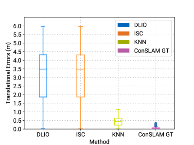
(a)

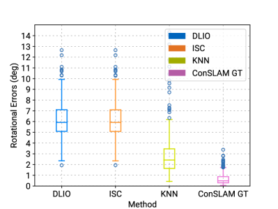
(b)

Figure 9: Translational (a) and rotational (b) errors for sequence 4 after alignment with the respective TLS point cloud.

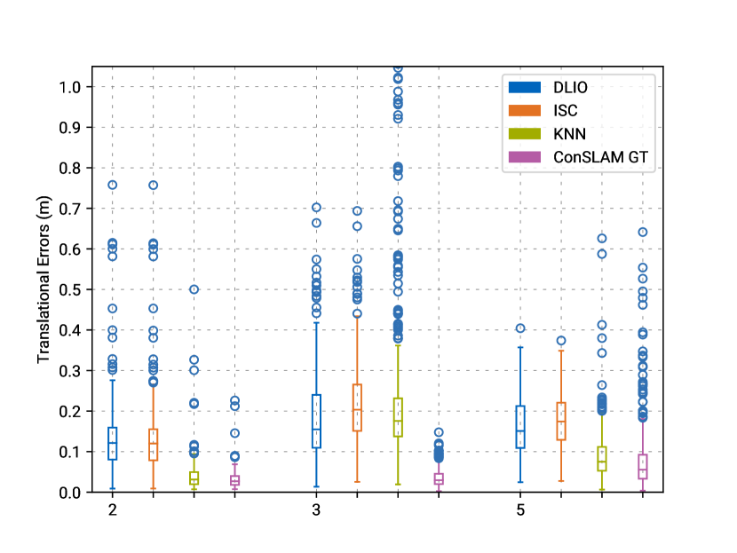
Figure 10: Translational errors for sequences 2, 3, and 5 after alignment with the respective TLS point clouds.

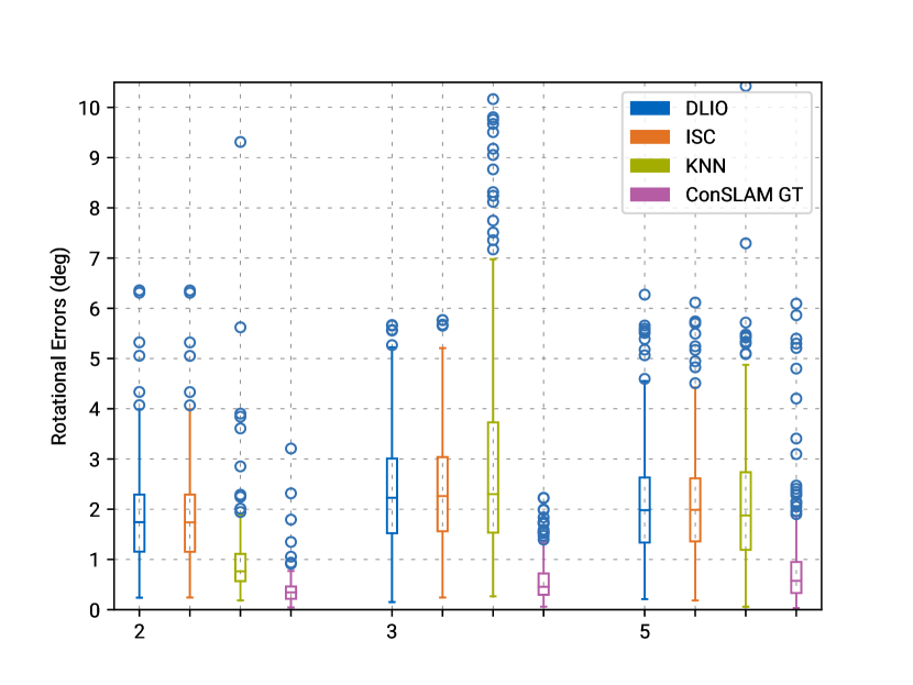
Figure 11: Rotational errors for sequences 2, 3, and 5 after alignment with the respective TLS point clouds.

Notably, the errors exhibit an evident reduction across almost all sequences while the pipeline evolves.

The ISC loops primarily allow the critical first rough alignment between the query and reference sessions. Since only a few ISC loops are retained due to rigorous threshold criteria, the outcomes after ISC loop detection and optimization exhibit minimal alteration in trajectory accuracy when compared to the initial results derived from DLIO.

On the other hand, the subsequent KNN loops exhibit a more pronounced impact on the results after ISC loops.

While the average rotational error, as depicted in Figure 11, experiences a significant decrease in sequences 2 and 4, it exhibits apparent stability or even an increase in sequences 3 and 5.

Regarding the GT poses provided with the ConSLAM dataset, although the RMSE for APE remains below 8 cm and 1 degree for translation and angular errors, respectively (as shown in the last column of Table 1), the maximum errors escalate to 20 or even 60 cm in sequences 2 and 5 (see Figure 10). While these significant discrepancies are in relatively small sections of the trajectories, it is also essential to recognize that for a LiDAR-based SLAM dataset, ground truth poses should ideally exhibit accuracy levels of at least one centimeter across the entire trajectory. This level of accuracy is now achievable in a highly automated manner with the proposed SLAM2REF framework.

Additionally, we demonstrate that it is possible to align and correct a 3D map using a BIM model as a reference map, despite significant deviations between the current map and the reference BIM model (Scan-Map deviations of the types 1 and 2 as stated in the introduction, see Section 1). This significant level of deviation is particularly evident in the context of the ConSLAM construction site. Figure 12 and 13 depicts the results after alignment with BIM. Here, the error values after the final ICP step are visible since they do not coincide with the ground truth poses anymore.

Similar to the alignment process with the TLS point cloud presented previously, the error does not decrease after ISC loops; however, it notably reduces after the final ICP step. The translational RMSE of the APE decreases to 14.8 cm, while the rotational RMSE is 0.56 degrees.

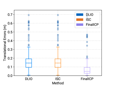
(a)

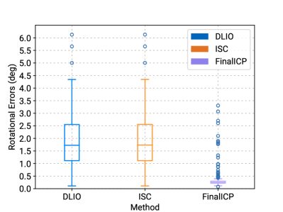
(b)

Figure 12: Translational (a) and rotational (b) errors for the sequence 2 after alignment with BIM model.

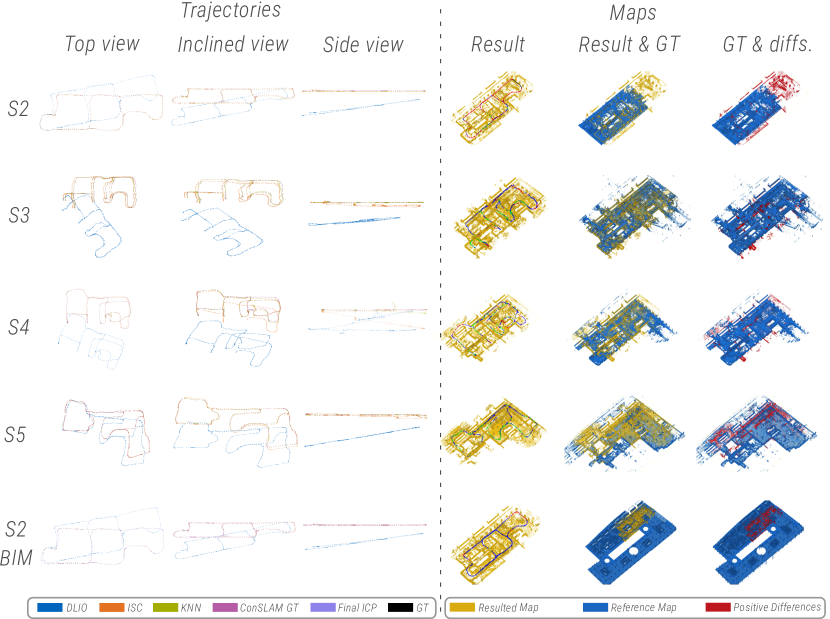
Figure 13: Trajectories and maps for sequences 2, 3, 4, and 5 after alignment with the respective TLS point clouds, and for sequence 2 after alignment with the BIM model. The trajectories of the first three columns correspond to the results of the different methods/steps, which have the same label colors as in Fig. 10. Additionally, the ground truth trajectory is shown in black. The trajectory in the fourth column displays points in different colors to indicate registration results: perfect (green), good (blue), bad (red), or outside of the map (black). In the fourth and fifth columns, the resulting map is shown in yellow, and the reference target map is shown in blue. In the last column, the differences (new elements in the resulting map) are depicted in red.

Regarding the results of Step 3, the identified positive changes are highlighted in red within the final column of Figure 13. Furthermore, Figures 14a and 14b provide detailed visualizations of the discrepancies observed in sequence 2 following alignment with both the TLS point cloud and the BIM model, respectively. While the disparities with the TLS point cloud are relatively minor, involving slight shifts in the positions of certain fences and construction resources, the distinctions when compared to the BIM model (Figure 14b) are notably substantial. This serves to exhibit the robustness of our alignment methodology in effectively accommodating considerable levels of Scan-BIM deviations.

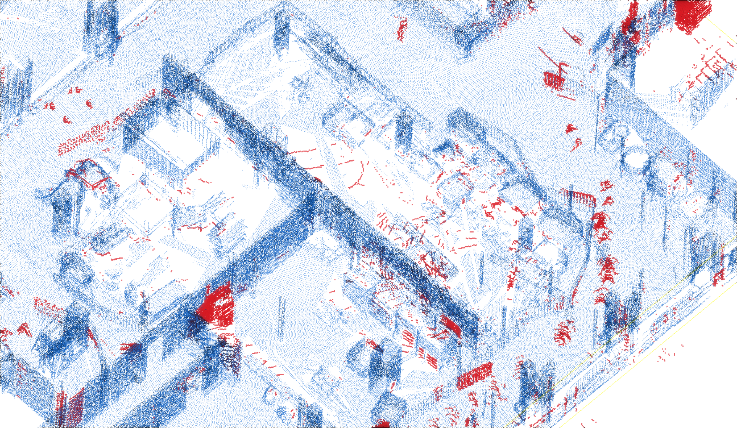
(a)

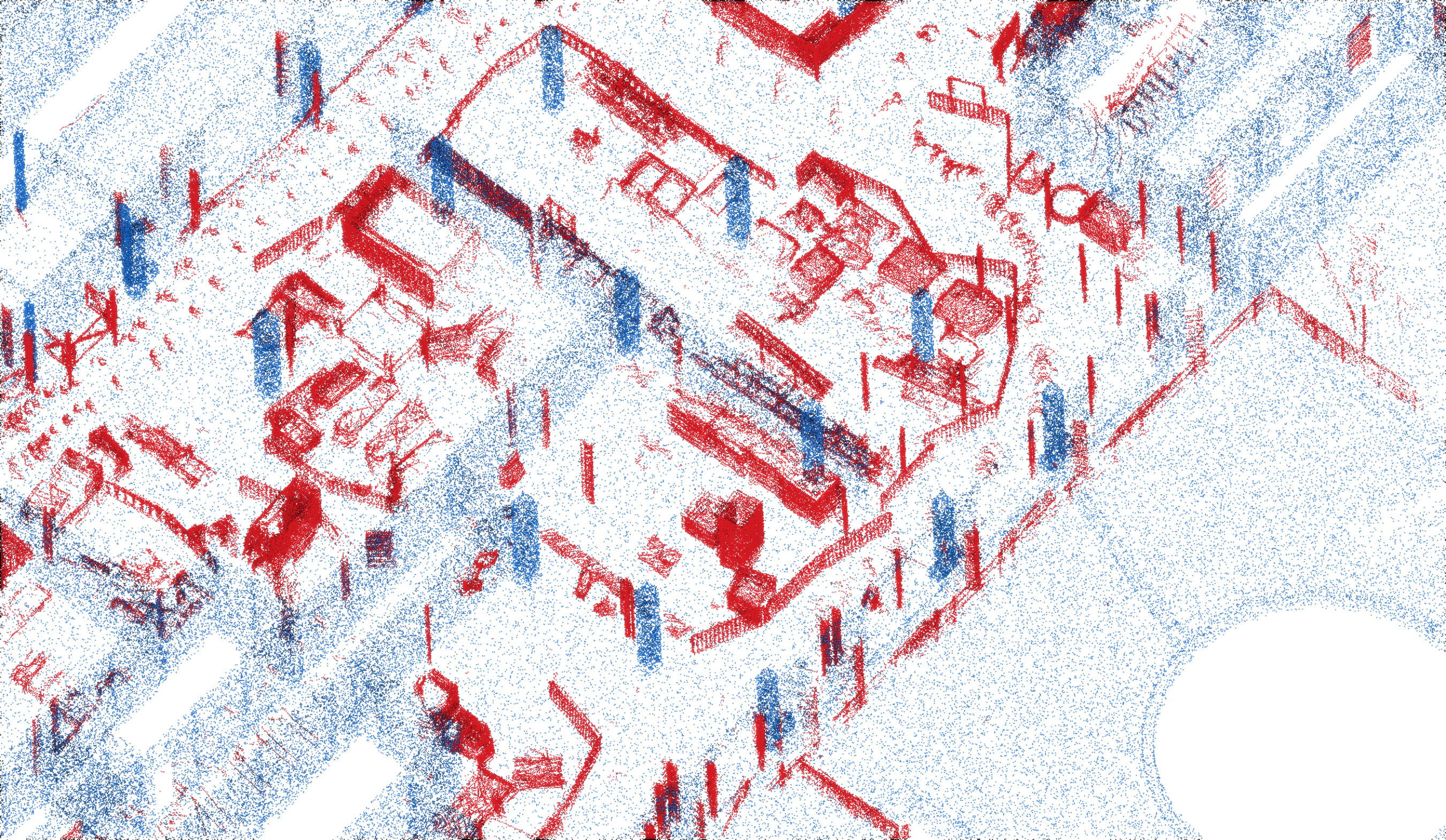
(b)

Figure 14: Change detection after map alignment. Both images correspond to the results of sequence 2: in (a), the sequence was compared against the respective TLS point cloud, and in (b) against the BIM model. The positive differences, i.e., new elements in the resulting map, are depicted in red.

7 Discussion

This section contains a more detailed interpretation of the results reported previously. Furthermore, we look into the motivation for our methodology and how it contributes to progress in this field of research, explaining the enhancements of our approach compared to prior works and outlining directions for future studies.

The apparently contradictory pattern of the rotational errors in sequences 2 and 5 can be attributed to the Umeyama alignment process [76]. In certain regions, the actual trajectory after ISC loop detection (without Umeyama alignment) deviates approximately 1.5 meters from the ground truth in the Z and X directions, leading to erroneous identification of KNN loops. Nonetheless, these erroneous loops are effectively identified and filtered out during the final ICP step.

One potential source of error for the ConSLAM GT poses lies in the MDC step. Contrary to common practice, the authors extracted the scans directly from the recorded bagfiles, omitting the deskewing process [74]. Avoiding the undistortion process can mislead any registration method, particularly affecting the accuracy of the calculated poses in sections where the trajectory was recorded under rapid motion.

The reason why KNN loops tend to yield incorrect correspondences during alignment with the SD from a BIM model can be attributed to Scan-Map deviations, as well as the absence of ceiling points in simulated scans from the BIM model. These facts complicate the registration of small sub-maps from the real world with sub-maps from a BIM model, particularly given that elements on the construction site have corners and features sometimes misinterpreted by the YawGICP registration process as permanent elements. Nonetheless, the final ICP method overcomes this challenge by utilizing a dense point cloud from the BIM model and relying solely on point-to-point (P2P) correspondences, thus avoiding estimating tangent planes for the alignment.

An alternative to simulating LiDAR scans (as done in section 4.1.3) could involve cropping a point cloud from the reference map within spheres as performed for the final ICP step (section 4.2.3). However, simulating scans offers a critical advantage: it enables the incorporation of only the geometry of elements visible from the scan’s origin. This visibility filter is crucial for ensuring the robustness of descriptor-based alignment in the ISC loop detection step, as only the information of single scans is compared here. Furthermore, when registering real-world scans with simulated ones, the process not only demonstrates quickness but also mitigates potential interference from double surfaces, such as from walls, as only the visible surfaces from the sensor origin are considered.

In comparison to our prior research [78] and other localization algorithms, SLAM2REF presents notable advantages. Since it enables the creation of a map and subsequent alignment with a reference map, unlike typical localization methods, our framework does not require the sensor to initiate mapping from within the map itself. Instead, it allows the sensor to start from any location, ensuring that the resulting map aligns with some overlapped regions of the reference map. Therefore, SLAM2REF also supports the extension of the reference map. This means that even if sensor measurements expand beyond the map boundaries, they are still aligned with the existing map in the most coherent manner.

Additionally, our pipeline does not necessitate any manual intervention to align the first keyframe, a process typically required by methods utilized to generate the ground truth poses in some of the latest datasets, such as in [75, 74, 68, 85]. Moreover, due to the initialization of our pipeline with SLAM or odometry-calculated poses and the optimized parallel registrations, our pipeline also enables the rapid retrieval of GT poses utilizing dense, accurate reference maps.

When contrasting with BIM-SLAM [79], SLAM2REF showcases several distinct advantages: Firstly, it is compatible with large-scale reference maps, encompassing not only large BIM models but also dense high-quality point clouds. Secondly, it effectively considers motion distortion in LiDAR data and mitigates it by leveraging IMU measurements. Thirdly, it achieves significantly improved accuracy in 6-DoF pose retrieval through the final ICP step and a TLS point cloud as a reference map. Lastly, our pipeline enables the alignment in the presence of Scan-Map deviation, such as with a BIM model, leveraging the proposed enhanced version of the Scan Context descriptor tailored for indoor environments.

Additionally, our pipeline operates independently of ROS or Gazebo (used previously for scan simulation).

Another remarkable characteristic of our method is its adaptability, as it is not restricted to Manhattan-world environments with enclosed rooms, as the method proposed by [72].

8 Achievements and limitations

As mentioned in the previous section, SLAM2REF enables the automatic alignment and correction of data with a reference map. This alignment can achieve high accuracy and map extension, even with Scan-Map deviations and in environments that do not follow the Manhattan-world assumption. Although meticulous attention has been given to its design, the proposed framework inherently has limitations that influence its effectiveness in aligning the new data with a reference map. This section elaborates on specific areas where the proposed methodology may encounter challenges.

One of the most critical limitations is the sensitivity to the initial poses calculated with the SLAM or LIO system. In scenarios where these poses exhibit significant displacement or drift from their correct positions, our pipeline may not be able to rectify them. One way to possibly overcome this issue might be to implement a second ISC loop detection with a radius-based search, following the first ISC loop closure detection. The first ISC loop will provide an initial coarse alignment of the trajectory, probably with only a few correspondences. Subsequently, the second ISC loop closure process will serve to correct parts of the trajectory that manifest substantial drift. However, it is worth noting that this approach may introduce wrong correspondences, particularly in cases with symmetric environments.

In particular, as depicted in Figure 15, when encountering a Z-drift within a narrow corridor, the limited information provided by individual scans regarding horizontal elements (such as floors or ceilings) can sometimes make automatic height retrieval very challenging. One possible approach to mitigate this issue involves the utilization of the free space, which can be calculated using OctoMap (as outlined in Section 4.3). Assuming most transition elements, such as doors and windows, are open during scanning, they could serve as reference elements for height retrieval by utilizing their frames as a feature for registration.

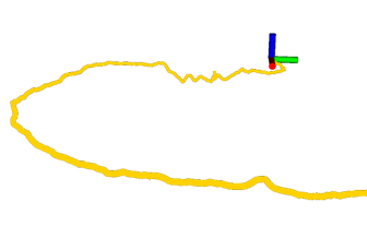
(a)

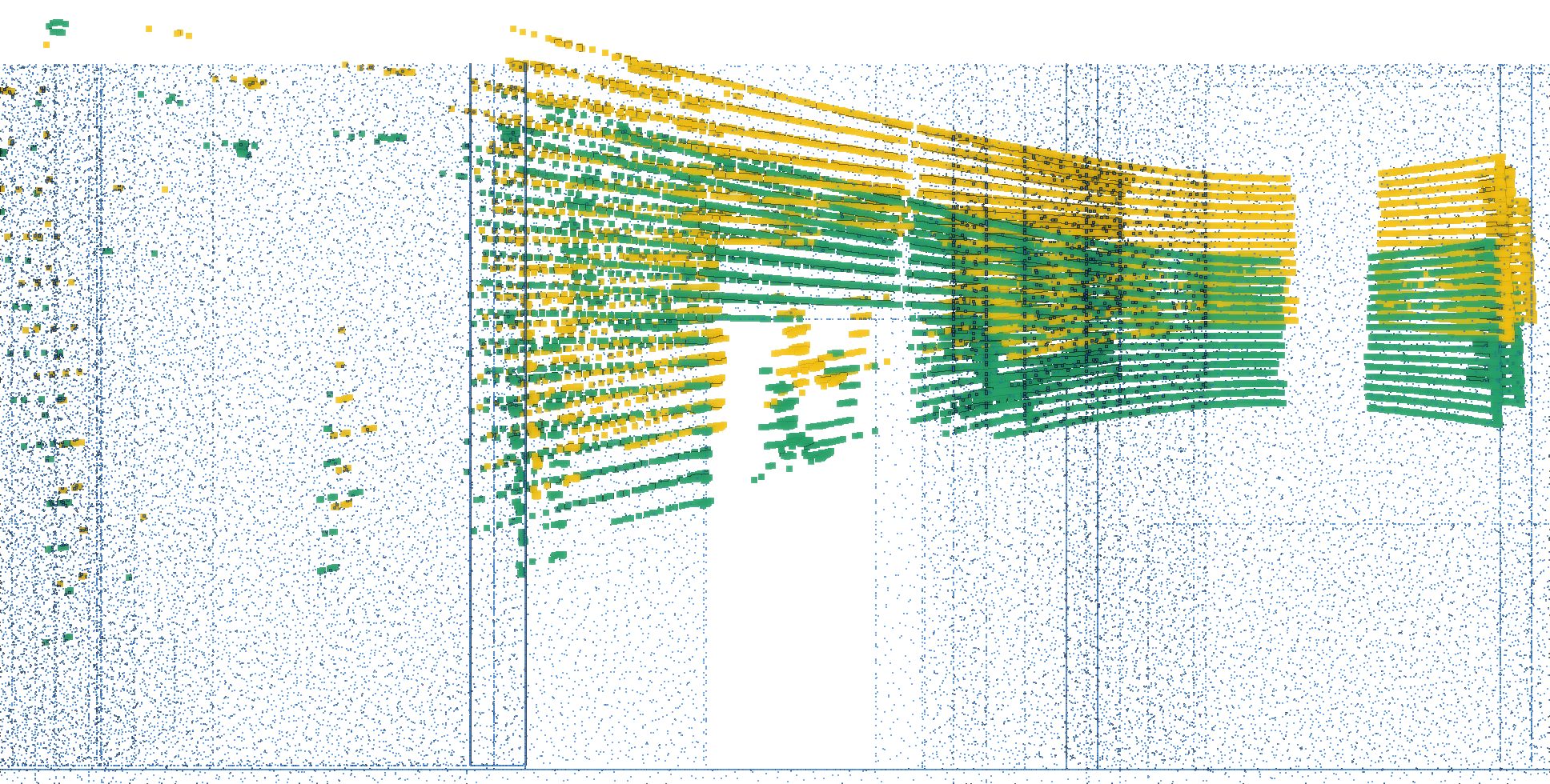
(b)

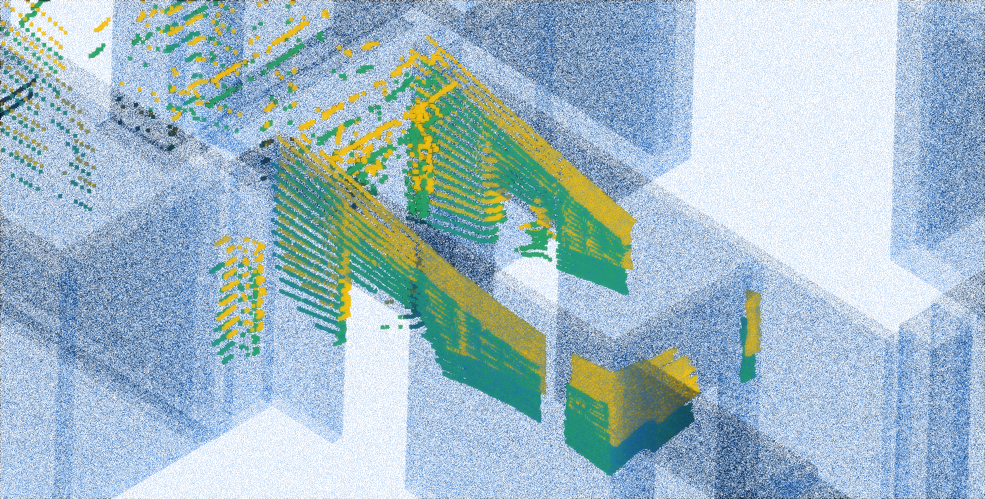
(c)

Figure 15: Limitation regarding the inaccuracy of initial poses: If the initially calculated poses drift in the Z direction, as depicted in (a), the final scan might not be automatically registered in the correct poses if they are located in narrow corridors. This occurs because specific scans, like the yellow one in (b) and (c), lack the ceiling or floor points necessary to determine the correct sensor height. (b) and (c) are the side and perspective views of the same scene. The green scan represents the manually correctly registered scan, while the blue depicts the reference map, in this case, a point cloud sampled from the BIM model.

Another limitation is related to the accuracy of the reference map. For instance, in scenarios characterized by substantial Scan-Map deviations—such as significant discrepancies in the positions of permanent walls and columns, minimal overlap between the scan and the reference map, or symmetrical environments—our method may encounter challenges in achieving accurate alignment.

Even if the alignment is possible, the final ICP step might not yield correct results in the regions where the reference map is erroneous and the alignment process passes the specified fitness thresholds. This and the previous one are the main reasons why the results of the alignment with the BIM model (shown in Figure 12) are not perfect.

Furthermore, the computational time can also be considered as a constraint. Given the requirements of high accuracy, our method does not achieve real-time performance, particularly during the final ICP step. This step involves registering individual scans with a dense point cloud, a process that can extend to several dozen minutes.

In addition, another constraint is evident in terms of the proposed ISCD and the corresponding loop detection step. This descriptor, as well as the family of egocentric or SC descriptors, are specifically designed to work with LiDAR scans from a sensor with a horizontal FoV of 360 deg. The reason behind this is mainly to be able to create rotational invariant 1D descriptors. Therefore, the pipeline is not directly compatible with data from sensors with a reduced FoV, such as solid-state LiDARs and depth cameras.

In Step 3, a primary limitation of our current pipeline emanate from reflections in window elements. As depicted in Figures 16a and 16b, these windows induce reflections in the LiDAR measurements, leading to the reconstruction of fictitious reflected elements within the detected changes. Specifically, the presence of reflected walls is noticeable in sequences 3, 4, and 5 (see last column of Figure 13. Notably, this issue is absent in sequence 2, attributed to the absence of window installations and the delimitation of the scan trajectory within the boundaries of walls with windows. To address this issue, one potential approach involves utilizing camera measurements to selectively filter out LiDAR measurements acquired in regions with window presence. Alternatively, a manual and more labor-intensive approach would involve physically occluding windows prior to scanning.

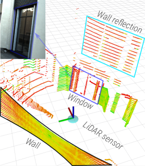
(a)

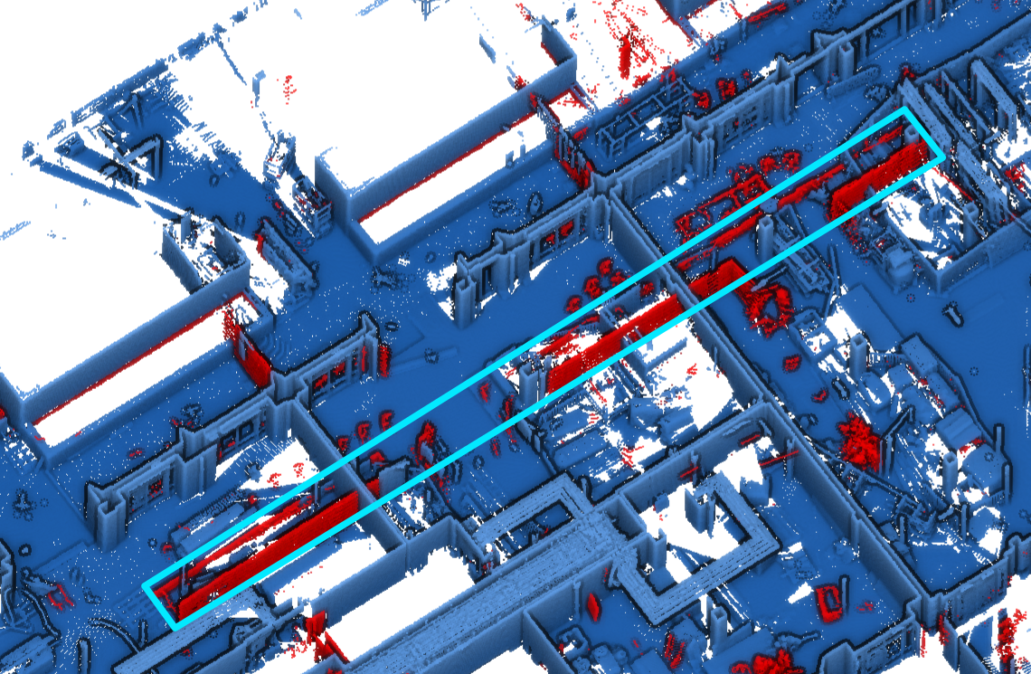
(b)

Figure 16: Limitation regarding wrongly detected changes following map alignment. In (a), the presence of reflective surfaces, such as windows, can lead to the generation of fictitious walls due to the LiDAR sensor’s inability to filter out reflected measurements. This is illustrated in the top left, where an image of the actual window causing reflections is depicted, while at the bottom, the LiDAR measurement captures the wall, window, and the reflected fictitious wall. In (b), these reflections result in inaccurately detected changes in sequences 3, 4, and 5.

9 Conclusions

This paper presents SLAM2REF, a modular framework to allow automatic 3D LiDAR data alignment and change detection with a reference map, which can be a BIM model or a point cloud.

The framework operates independently of the sensor’s initial position, eliminating the necessity for the scanning process to start within the provided map boundaries. Consequently, our framework enables map alignment and extension even when the reference map is outside the field of view (FoV) of the sensor or if only a portion of the map has been scanned.

Moreover, if an accurate TLS point cloud is available, it can serve as a reference map to correct the poses of a query session and even retrieve centimeter-accurate ground truth poses.

More specifically, the following are our main contributions:

• A method to extract OGMs out of complex BIM models or large-scale point clouds, which could serve to allow robot path planning and autonomous navigation in indoor GPS-denied environments.

• An efficient method to convert large-scale 3D maps into session data for fast 3D-LiDAR place recognition.

• A module that leverages quick place recognition and multi-session anchoring to allow the alignment and correction of drifted session acquired with SLAM or odometry systems, given the presence of a reference map and considering motion distortion correction as in [14].

• Provided that the reference map is accurate enough, the framework enables the retrieval of precise 6-DoF poses of the entire trajectory, also enabling map extension.

• We introduced YawGICP, a robust implementation of GICP tailored to effectively address registration problems primarily characterized by yaw angle variations.

• Similarly, we introduce ISC, an innovative 2D descriptor that allows the alignment of the data with BIM models in scenarios with Scan-Map deviations.

• We present an extensive quantitative comparison of the steps in the pipeline, considering a state-of-the-art 3DLiDAR-inertial odometry algorithm for pose initialization and exploiting the multiple sequences of the real-world open-access ConSLAM dataset.

• Finally, we provide a module that can detect positive and negative differences (i.e., when parts of the original reference map are no longer present in the environment) in the aligned map and create surfaces for better visualization with the BIM model or reference point cloud.

These functionalities collectively contribute to facilitating resilient long-term map data management, consolidating aligned relevant 3D information within a unified reference coordinate system.

In conclusion, SLAM2REF offers a novel solution to the challenges of lifelong mapping by integrating 3D LiDAR data and IMU measurements with a reference map, enabling automatic alignment, precise 6-DoF trajectory estimation, map extension, and change detection.

By allowing Scan-Map deviations, SLAM2REF offers a robust solution for automated 3D data alignment, even with as-designed BIM models that typically have significant deviations from as-built environments.

Our approach provides indirect support for the development of Digital Twins (DTs) for buildings, allowing the automatic alignment of newly acquired data with digital models. These models require continuous data integration to maintain its accuracy and relevance.

Practical applications are found in areas such as construction site monitoring, emergency response, disaster management, and others, where fast-updated digital 3D maps contribute to better decision-making and productivity.

Furthermore, since our method is capable of exploiting BIM models that are semantically enhanced or point clouds as reference maps for localization, it can be used to support the development of autonomous robotic activities.

Another advantage of SLAM2REF is that it advances SLAM research by enabling the automatic retrieval of centimeter-level accurate 6-DoF GT poses for large-scale indoor and outdoor trajectories.

10 Future Directions

In the future, we would like to extend the method, considering calibrated camera data, to leverage semantics from the real world, such as done by [86]. By enriching camera measurements with semantic information, we anticipate better mitigation of the window reflection issue illustrated in Figure 16a. Additionally, an extended framework that is able to handle the alignment and correction of data with a reduced FoV would allow it to work with data captured from solid-state LiDARs or depth cameras.

Further validation on more datasets, such as the Newer College [68, 85], or the Hilti [87] datasets, would give more insights into the robustness of the method.

Moreover, extending the efficiency and robustness of the method towards a real-time pipeline represents a promising direction for various tasks, including collaborative robot mapping and localization [12, 50], such as to be able to solve the kidnapping robot problem in indoor environments with our proposed ISC descriptor. An essential aspect of achieving more robust alignment involves leveraging deep-learning-based place recognition algorithms, which are anticipated to become progressively reliable for indoor scenarios with sufficient training data in the future.

11 Acknowledgement

The presented research was conducted in the frame of the project “Intelligent Toolkit for Reconnaissance and assessmEnt in Perilous Incidents” (INTREPID) funded by the EU’s research and innovation funding programme Horizon 2020 under Grant agreement ID: 883345, as well as by the TUM Georg Nemetschek Institute in the frame of the AI4TWINNING project.

Appendix A Appendix

The table below lists the mathematical variables used in this manuscript, along with their corresponding descriptions.

Table 2: Explanation of Variables

Variable	Description
$p(X|z)$	Posterior density of the states $X$ given the measurements $Z$.
$F=(\mathcal{U},\mathcal{V},\mathcal{E})$	Factor graph comprising nodes ($x_{i}$ or $\phi_{i}$) connected by edges $e_{ij}$.
$\mathcal{E}$	Set of factor edges $e_{ij}$.
$\mathcal{U}$	Set of factor nodes $\phi_{i}$.
$\mathcal{V}$	Set of variable nodes $x_{i}$.
$X_{i}$	Group of variables $x_{i}$ connected to a factor $\phi_{i}$.
$\phi(X)$	Global function factorized as $\phi(X)=\prod_{i}\phi_{i}(X_{i})$.
$z_{i}$	Measurements (observed data point or variable).
$h_{i}(x_{i},l_{i})$	Mean measurement function of $x_{i}$ and $l_{i}$. Represents the expected value of $z_{i}$ given $x_{i}$ and $l_{i}$.
$\Sigma_{i}$	Covariance matrix associated with $z_{i}$, representing zero-mean Gaussian noise.
$p(z_{i}|x_{i},l_{i})$	Conditional density on the measurement $z_{i}$.
$\mathcal{N}(z_{i};h_{i}(x_{i},l_{i}),\Sigma_{i})$	Multivariate normal distribution for the variable $z_{i}$ with mean $h_{i}(x_{i},l_{i})$ and covariance matrix $\Sigma_{i}$.
$\left\|h_{i}(x_{i},l_{i})-z_{i}\right\|_{\Sigma_{i}}^{2}$	Mahalanobis distance between $z_{i}$ and its mean $h_{i}(x_{i},l_{i})$.
$\mathrm{SE}(3)$	Special Euclidean group.
$\eta$	Normally distributed zero-mean measurement noise with covariance $\Sigma_{c}$.
$\mathcal{S_{R}}$	Synthetic reference session (created in Step 1, Section 4.1).
$\mathcal{S_{Q}}$	Real-world motion-undistorted query session (created in Step 2.1, Section 4.2.1).
$\mathbf{x}_{R}$	Set of poses of the reference session.
$\mathbf{x}_{Q}$	Set of poses of the query session.
$f(\cdot)$	Odometry model function.
$\mathbf{u}_{i}^{s}$	Constraints between consecutive poses $\mathbf{x}_{i}$ and $\mathbf{x}_{i+1}$.
$M_{s}$	Number of poses in the session $\mathcal{S}$.
$N_{e}$	Number of encounters between sessions.
$\mathbf{p}_{s}$	Prior factor.
$\Delta_{Q}^{*}$	Anchor node which facilitates the global alignment of the query session to the reference map.
$\mathcal{G}$	Pose-graph map containing coordinates of pose nodes, odometry edges, and optionally recognized intra-session loop edges with uncertainty matrices.
$\left(\mathcal{P}_{i},d_{i}\right)$	Pairs of 3D LiDAR scans $\mathcal{P}_{i}$ with their corresponding global descriptors $d_{i}$ of the $i^{th}$ keyframe.
$n$	Total number of equidistantly sampled keyframes.
$N_{c}$	Amount of Top descriptors candidates selected from the reference session after the comparison of the rotational invariant descriptors.
$\Sigma_{c}$	Covariance matrix of the detected loops or encounters incorporated into the factor graph problem as factors between sessions with anchoring.
$\mathbf{x}_{Q}^{*}$	Optimized 6-DoF poses of each scan of the query session.
$\mathbf{c}$	Loop closure detections, also called encounters denoting correspondences between the sessions.
$\mathbf{\nu}_{Q}$	Confidence level list providing the reliability of each pose after scan registration.
$h(\cdot)$	Original measurement model.
$h^{\prime}(\cdot)$	Modified measurement model that incorporates anchor nodes.
$\mathbf{x}_{R,j}$	6-DoF (in $\mathrm{SE}(3)$) Pose $j$ in the reference session.
$\mathbf{x}_{Q,j}$	6-DoF (in $\mathrm{SE}(3)$) Pose $j$ in the query session.
$\Delta_{R}$	Anchor node for the reference session (also in (in $\mathrm{SE}(3)$).
$\Delta_{Q}$	Anchor node for the query session (in $\mathrm{SE}(3)$).
$\mathbf{c}_{j}$	Difference in the global frame between poses $\mathbf{x}_{R}$ and $\mathbf{x}_{Q}$ (pose in $\mathrm{SE}(3)$).
$\oplus$	$\mathrm{SE}(3)$ pose composition operator.
$\ominus$	$\mathrm{SE}(3)$ pose difference operator.
$\phi(\mathbf{x}_{R,i},\mathbf{x}_{Q,j},\Delta_{R},\Delta_{Q})$	Factor between sessions with anchoring, used in pose graph optimization.
$\Sigma_{P}$	Covariance assigned to the anchor node of the reference session, set to be insignificantly small.
$\Sigma_{L}$	Covariance assigned to the anchor node of the query session, set to be significantly large.
${}^{Q}\mathbf{x}_{Q}^{*}$	Optimized poses of the query session in the local coordinate system.
${}^{W}\mathbf{x}_{Q}^{*}$	Optimized poses of the query session transformed to the global coordinate system of the reference map.
$W$	Global coordinate system, same as the coordinate system of the reference session.
$F_{i}$	Fitness score distance threshold. The fitness score is the percentage of source inliers after point cloud registration, considering a maximum Point-to-Point (P2P) distance threshold.

References

- \bibcommenthead
- Alliez et al. [2020] Alliez, P., Bonardi, F., Bouchafa, S., Didier, J.-Y., Hadj-Abdelkader, H., Muñoz, F.I., Kachurka, V., Rault, B., Robin, M., Roussel, D.: Real-time multi-slam system for agent localization and 3d mapping in dynamic scenarios. In: 2020 IEEE/RSJ International Conference on Intelligent Robots and Systems (IROS), pp. 4894–4900 (2020). IEEE
- Borrmann et al. [2024] Borrmann, A., Biswanath, M., Braun, A., Chen, Z., Cremers, D., Heeramaglore, M., Hoegner, L., Mehranfar, M., Kolbe, T.H., Petzold, F., Rueda, A., Solonets, S., Zhu, X.X.: Artificial intelligence for the automated creation of multi-scale digital twins of the built world—ai4twinning. In: Kolbe, T.H., Donaubauer, A., Beil, C. (eds.) Recent Advances in 3D Geoinformation Science, pp. 233–247. Springer, Cham (2024)
- Boniardi et al. [2017] Boniardi, F., Caselitz, T., Kummerle, R., Burgard, W.: Robust lidar-based localization in architectural floor plans. In: 2017 IEEE/RSJ International Conference on Intelligent Robots and Systems (IROS), pp. 3318–3324. IEEE, Vancouver, BC, Canada (2017). https://doi.org/10.1109/IROS.2017.8206168
- Boniardi et al. [2019] Boniardi, F., Caselitz, T., Kümmerle, R., Burgard, W.: A pose graph-based localization system for long-term navigation in cad floor plans. Robotics and Autonomous Systems 112, 84–97 (2019) https://doi.org/10.1016/j.robot.2018.11.003
- Blanco-Claraco [2021] Blanco-Claraco, J.L.: A tutorial on transformation parameterizations and on-manifold optimization. CoRR abs/2103.15980 (2021) 2103.15980
- Besl and McKay [1992] Besl, P.J., McKay, N.D.: A method for registration of 3-d shapes. IEEE Transactions on Pattern Analysis and Machine Intelligence 14(2), 239–256 (1992) https://doi.org/%****␣main.bbl␣Line␣150␣****10.1109/34.121791
- Blum et al. [2021] Blum, H., Milano, F., Zurbrügg, R., Siegwart, R., Cadena, C., Gawel, A.: Self-improving semantic perception on a construction robot. CoRR abs/2105.01595 (2021) 2105.01595
- Blanco and Rai [2014] Blanco, J.L., Rai, P.K.: nanoflann: a C++ header-only fork of FLANN, a library for Nearest Neighbor (NN) wih KD-trees (2014)
- Blum et al. [2020] Blum, H., Stiefel, J., Cadena, C., Siegwart, R., Gawel, A.: Precise robot localization in architectural 3d plans. arXiv preprint arXiv:2006.05137 (2020)
- Botín-Sanabria et al. [2022] Botín-Sanabria, D.M., Mihaita, A.-S., Peimbert-García, R.E., Ramírez-Moreno, M.A., Ramírez-Mendoza, R.A., Lozoya-Santos, J.d.J.: Digital twin technology challenges and applications: A comprehensive review. Remote Sensing 14(6) (2022) https://doi.org/10.3390/rs14061335
- Bai et al. [2022] Bai, C., Xiao, T., Chen, Y., Wang, H., Zhang, F., Gao, X.: Faster-lio: Lightweight tightly coupled lidar-inertial odometry using parallel sparse incremental voxels. IEEE Robotics and Automation Letters 7(2), 4861–4868 (2022) https://doi.org/10.1109/LRA.2022.3152830
- Cramariuc et al. [2022] Cramariuc, A., Bernreiter, L., Tschopp, F., Fehr, M., Reijgwart, V., Nieto, J., Siegwart, R., Cadena, C.: maplab 2.0–a modular and multi-modal mapping framework. IEEE Robotics and Automation Letters (2022)
- Caballero and Merino [2021] Caballero, F., Merino, L.: Dll: Direct LiDAR localization. a map-based localization approach for aerial robots. In: 2021 IEEE/RSJ International Conference on Intelligent Robots and Systems (IROS), pp. 5491–5498 (2021). IEEE
- Chen et al. [2023] Chen, K., Nemiroff, R., Lopez, B.T.: Direct lidar-inertial odometry: Lightweight lio with continuous-time motion correction. In: 2023 IEEE International Conference on Robotics and Automation (ICRA), pp. 3983–3989 (2023). IEEE
- Chen et al. [2024] Chen, Z., Xu, Y., Yuan, S., Xie, L.: ig-lio: An incremental gicp-based tightly-coupled lidar-inertial odometry. IEEE Robotics and Automation Letters, 1–8 (2024) https://doi.org/10.1109/LRA.2024.3349915
- Dugstad et al. [2022] Dugstad, A., Dubey, R.K., Abualdenien, J., Borrmann, A.: BIM-based disaster response: Facilitating indoor path planning for various agents. In: Proc. of European Conference on Product and Process Modeling 2022, pp. 265–289 (2022)
- Dellaert [2021] Dellaert, F.: Factor graphs: Exploiting structure in robotics. Annual Review of Control, Robotics, and Autonomous Systems 4, 141–166 (2021)
- Dellaert et al. [2017] Dellaert, F., Kaess, M., et al.: Factor graphs for robot perception. Foundations and Trends in Robotics 6(1-2), 1–139 (2017)
- de Teruel et al. [2017] Lopez-de-Teruel, P.E., Garcia, F.J., Canovas, O., Gonzalez, R., Carrasco, J.A.: Human behavior monitoring using a passive indoor positioning system: a case study in a sme. Procedia Computer Science 110, 182–189 (2017) https://doi.org/10.1016/j.procs.2017.06.076 . 14th International Conference on Mobile Systems and Pervasive Computing (MobiSPC 2017) / 12th International Conference on Future Networks and Communications (FNC 2017) / Affiliated Workshops
- Ercan et al. [2020] Ercan, S., Blum, H., Gawel, A., Siegwart, R., Gramazio, F., Kohler, M.: Online synchronization of building model for on-site mobile robotic construction. In: 37th International Symposium on Automation and Robotics in Construction (ISARC 2020)(virtual), pp. 1508–1514 (2020). International Association for Automation and Robotics in Construction
- Forster et al. [2016] Forster, C., Carlone, L., Dellaert, F., Scaramuzza, D.: On-manifold preintegration for real-time visual–inertial odometry. IEEE Transactions on Robotics 33(1), 1–21 (2016)
- Follini et al. [2020] Follini, C., Magnago, V., Freitag, K., Terzer, M., Marcher, C., Riedl, M., Giusti, A., Matt, D.T.: BIM-integrated collaborative robotics for application in building construction and maintenance. Robotics 10(1), 2 (2020) https://doi.org/10.3390/robotics10010002
- Gawel et al. [2019] Gawel, A., Blum, H., Pankert, J., Krämer, K., Bartolomei, L., Ercan, S., Farshidian, F., Chli, M., Gramazio, F., Siegwart, R., et al.: A fully-integrated sensing and control system for high-accuracy mobile robotic building construction. In: 2019 IEEE/RSJ International Conference on Intelligent Robots and Systems (IROS), pp. 2300–2307 (2019). IEEE
- Gschwandtner et al. [2011] Gschwandtner, M., Kwitt, R., Uhl, A., Pree, W.: Blensor: Blender sensor simulation toolbox. In: Bebis, G., Boyle, R., Parvin, B., Koracin, D., Wang, S., Kyungnam, K., Benes, B., Moreland, K., Borst, C., DiVerdi, S., Yi-Jen, C., Ming, J. (eds.) Advances in Visual Computing, pp. 199–208. Springer, Berlin, Heidelberg (2011)
- Geiger et al. [2013] Geiger, A., Lenz, P., Stiller, C., Urtasun, R.: Vision meets robotics: The kitti dataset. International Journal of Robotics Research (IJRR) (2013)
- Grupp [2017] Grupp, M.: evo: Python package for the evaluation of odometry and SLAM. https://github.com/MichaelGrupp/evo (2017)
- Gschwandtner [2013] Gschwandtner, M.: Support framework for obstacle detection on autonomous trains. PhD thesis, Department of Computer Sciences, University of Salzburg (2013)
- Hendrikx et al. [2022] Hendrikx, R., Bruyninckx, H., Elfring, J., Van De Molengraft, M.: Local-to-global hypotheses for robust robot localization. Frontiers in Robotics and AI, 171 (2022)
- Hess et al. [2016] Hess, W., Kohler, D., Rapp, H., Andor, D.: Real-time loop closure in 2d LiDAR SLAM. In: 2016 IEEE International Conference on Robotics and Automation (ICRA), pp. 1271–1278. IEEE, Stockholm, Sweden (2016). https://doi.org/10.1109/ICRA.2016.7487258
- Hendrikx et al. [2021] Hendrikx, R.W.M., Pauwels, P., Torta, E., Bruyninckx, H.J.P., van de Molengraft, M.J.G.: Connecting semantic building information models and robotics: An application to 2d lidar-based localization. In: 2021 IEEE International Conference on Robotics and Automation (ICRA), pp. 11654–11660. IEEE, Xi’an, China (2021). https://doi.org/10.1109/ICRA48506.2021.9561129
- Hornung et al. [2013] Hornung, A., Wurm, K.M., Bennewitz, M., Stachniss, C., Burgard, W.: Octomap: An efficient probabilistic 3d mapping framework based on octrees. Autonomous robots 34, 189–206 (2013)
- He et al. [2021] He, G., Zhang, F., Li, X., Shang, W.: Robust mapping and localization in offline 3d point cloud maps. In: 2021 6th IEEE International Conference on Advanced Robotics and Mechatronics (ICARM), pp. 765–770 (2021). https://doi.org/10.1109/ICARM52023.2021.9536181
- IfcOpenShell Contributors [2023a] IfcOpenShell Contributors: IfcConvert: An application for converting IFC geometry into several file formats. Software. URL: https://ifcopenshell.sourceforge.net/ifcconvert.html (2023). https://ifcopenshell.sourceforge.net/ifcconvert.html
- IfcOpenShell Contributors [2023b] IfcOpenShell Contributors: Ifcconvert documentation. Online. URL: https://blenderbim.org/docs-python/ifcconvert/usage.html (2023). https://blenderbim.org/docs-python/ifcconvert/usage.html
- Jurić et al. [2021] Jurić, A., Kendeš, F., Marković, I., Petrović, I.: A comparison of graph optimization approaches for pose estimation in SLAM. In: 2021 44th International Convention on Information, Communication and Electronic Technology (MIPRO), pp. 1113–1118 (2021). https://doi.org/10.23919/MIPRO52101.2021.9596721
- Karimi et al. [2021] Karimi, S., Braga, R.G., Iordanova, I., St-Onge, D.: Semantic Navigation Using Building Information on Construction Sites (2021). http://arxiv.org/pdf/2104.10296v1
- Kim et al. [2021] Kim, G., Choi, S., Kim, A.: Scan context++: Structural place recognition robust to rotation and lateral variations in urban environments. IEEE Transactions on Robotics 38(3), 1856–1874 (2021)
- Koenig and Howard [2004] Koenig, N., Howard, A.: Design and use paradigms for gazebo, an open-source multi-robot simulator. In: 2004 IEEE/RSJ International Conference on Intelligent Robots and Systems (IROS)(IEEE Cat. No. 04CH37566), vol. 3, pp. 2149–2154 (2004). IEEE
- Karimi et al. [2020] Karimi, S., Iordanova, I., St-Onge, D.: An ontology-based approach to data exchanges for robot navigation on construction sites. Journal of Information Technology in Construction (2020)
- Kim and Kim [2018] Kim, G., Kim, A.: Scan context: Egocentric spatial descriptor for place recognition within 3d point cloud map. In: 2018 IEEE/RSJ International Conference on Intelligent Robots and Systems (IROS), pp. 4802–4809 (2018). IEEE
- Kim and Kim [2022] Kim, G., Kim, A.: Lt-mapper: A modular framework for lidar-based lifelong mapping. In: 2022 International Conference on Robotics and Automation (ICRA), pp. 7995–8002 (2022). IEEE
- Kim et al. [2010] Kim, B., Kaess, M., Fletcher, L., Leonard, J., Bachrach, A., Roy, N., Teller, S.: Multiple relative pose graphs for robust cooperative mapping. In: 2010 IEEE International Conference on Robotics and Automation, pp. 3185–3192 (2010). IEEE
- Koide et al. [2022] Koide, K., Oishi, S., Yokozuka, M., Banno, A.: Scalable fiducial tag localization on a 3d prior map via graph-theoretic global tag-map registration. In: 2022 IEEE/RSJ International Conference on Intelligent Robots and Systems (IROS), pp. 5347–5353 (2022). https://doi.org/10.1109/IROS47612.2022.9981079
- Kim and Peavy [2022] Kim, K., Peavy, M.: BIM-based semantic building world modeling for robot task planning and execution in built environments. Automation in Construction 138, 104247 (2022) https://doi.org/10.1016/j.autcon.2022.104247
- Kim et al. [2021] Kim, S., Peavy, M., Huang, P.-C., Kim, K.: Development of BIM-integrated construction robot task planning and simulation system. Automation in Construction 127, 103720 (2021) https://doi.org/10.1016/j.autcon.2021.103720
- Krijnen [2015] Krijnen, T.: IfcOpenShell (2015). https://github.com/IfcOpenShell/IfcOpenShell
- Kayhani et al. [2023] Kayhani, N., Schoellig, A., McCabe, B.: Perception-aware tag placement planning for robust localization of uavs in indoor construction environments. Journal of Computing in Civil Engineering 37(2) (2023) https://doi.org/10.1061/JCCEE5.CPENG-5068 . Cited by: 1; All Open Access, Green Open Access
- Kim et al. [2022] Kim, G., Yun, S., Kim, J., Kim, A.: Sc-lidar-slam: A front-end agnostic versatile lidar SLAM system. In: 2022 International Conference on Electronics, Information, and Communication (ICEIC), pp. 1–6 (2022). https://doi.org/10.1109/ICEIC54506.2022.9748644
- Kayhani et al. [2022] Kayhani, N., Zhao, W., McCabe, B., Schoellig, A.P.: Tag-based visual-inertial localization of unmanned aerial vehicles in indoor construction environments using an on-manifold extended kalman filter. Automation in Construction 135, 104112 (2022) https://doi.org/10.1016/j.autcon.2021.104112
- Lajoie and Beltrame [2024] Lajoie, P.-Y., Beltrame, G.: Swarm-slam: Sparse decentralized collaborative simultaneous localization and mapping framework for multi-robot systems. IEEE Robotics and Automation Letters 9(1), 475–482 (2024) https://doi.org/10.1109/lra.2023.3333742
- Liu et al. [2021] Liu, Y., Fu, Y., Chen, F., Goossens, B., Tao, W., Zhao, H.: Simultaneous localization and mapping related datasets: A comprehensive survey. arXiv preprint arXiv:2102.04036 (2021)
- Lee et al. [1994] Lee, T.-C., Kashyap, R.L., Chu, C.-N.: Building skeleton models via 3-d medial surface axis thinning algorithms. CVGIP: Graphical Models and Image Processing 56(6), 462–478 (1994)
- Li et al. [2021] Li, L., Kong, X., Zhao, X., Huang, T., Li, W., Wen, F., Zhang, H., Liu, Y.: Ssc: Semantic scan context for large-scale place recognition. In: 2021 IEEE/RSJ International Conference on Intelligent Robots and Systems (IROS), pp. 2092–2099 (2021). IEEE
- Lv et al. [2020] Lv, J., Xu, J., Hu, K., Liu, Y., Zuo, X.: Targetless Calibration of Lidar-imu System Based on Continuous-time Batch Estimation. In: 2020 IEEE/RSJ International Conference on Intelligent Robots and Systems (IROS), pp. 9968–9975 (2020). IEEE
- Lv et al. [2022] Lv, J., Zuo, X., Hu, K., Xu, J., Huang, G., Liu, Y.: OA-LICalib: Observability-aware intrinsic and extrinsic calibration of lidar-imu systems. IEEE Transactions on Robotics 38(6), 3734–3753 (2022)
- Macenski and Jambrecic [2021] Macenski, S., Jambrecic, I.: Slam toolbox: SLAM for the dynamic world. Journal of Open Source Software 6(61), 2783 (2021) https://doi.org/10.21105/joss.02783
- McDonald et al. [2013] McDonald, J., Kaess, M., Cadena, C., Neira, J., Leonard, J.J.: Real-time 6-dof multi-session visual SLAM over large-scale environments. Robotics and Autonomous Systems 61(10), 1144–1158 (2013) https://doi.org/10.1016/j.robot.2012.08.008 . Selected Papers from the 5th European Conference on Mobile Robots (ECMR 2011)
- Mylonas et al. [2021] Mylonas, G., Kalogeras, A., Kalogeras, G., Anagnostopoulos, C., Alexakos, C., Muñoz, L.: Digital twins from smart manufacturing to smart cities: A survey. IEEE Access 9, 143222–143249 (2021) https://doi.org/10.1109/ACCESS.2021.3120843
- Macenski et al. [2023] Macenski, S., Moore, T., Lu, D.V., Merzlyakov, A., Ferguson, M.: From the desks of ROS maintainers: A survey of modern & capable mobile robotics algorithms in the robot operating system 2. Robotics and Autonomous Systems 168, 104493 (2023) https://doi.org/10.1016/j.robot.2023.104493
- Moura et al. [2021] Moura, M.S., Rizzo, C., Serrano, D.: BIM-based Localization and Mapping for Mobile Robots in Construction. 2021 IEEE International Conference on Autonomous Robot Systems and Competitions, ICARSC 2021, 12–18 (2021) https://doi.org/10.1109/ICARSC52212.2021.9429779
- Macenski et al. [2023] Macenski, S., Singh, S., Martín, F., Ginés, J.: Regulated pure pursuit for robot path tracking. Autonomous Robots, 1–10 (2023)
- NavVis et al. [2022] NavVis, News, L., Magazine, L., American Surveyor, GoGeomatics, International, G., Week, G., BIMplus, Source, S., GeoConnexion: State of Mobile Mapping Survey 2022. NavVis (2022)
- Ozog et al. [2016] Ozog, P., Carlevaris-Bianco, N., Kim, A., Eustice, R.M.: Long-term mapping techniques for ship hull inspection and surveillance using an autonomous underwater vehicle. Journal of Field Robotics 33(3), 265–289 (2016)
- Oelsch et al. [2021] Oelsch, M., Karimi, M., Steinbach, E.: R-LOAM: Improving LiDAR Odometry and Mapping with Point-to-Mesh Features of a Known 3D Reference Object. IEEE Robotics and Automation Letters 6(2), 2068–2075 (2021) https://doi.org/10.1109/LRA.2021.3060413
- Oelsch et al. [2022] Oelsch, M., Karimi, M., Steinbach, E.: Ro-loam: 3d reference object-based trajectory and map optimization in lidar odometry and mapping. IEEE Robotics and Automation Letters, 1–1 (2022) https://doi.org/10.1109/LRA.2022.3177846
- Prieto et al. [2020] Prieto, S.A., Garcia de Soto, B., Adan, A.: A methodology to monitor construction progress using autonomous robots. In: Osumi, H. (ed.) Proceedings of the 37th International Symposium on Automation and Robotics in Construction (ISARC). Proceedings of the International Symposium on Automation and Robotics in Construction (IAARC), pp. 265–289. International Association for Automation and Robotics in Construction (IAARC), Tokyo, Japan (2020). https://doi.org/10.22260/ISARC2020/0210
- Perez-Grau et al. [2017] Perez-Grau, F.J., Caballero, F., Viguria, A., Ollero, A.: Multi-sensor three-dimensional monte carlo localization for long-term aerial robot navigation. International Journal of Advanced Robotic Systems 14(5) (2017) https://doi.org/10.1177/1729881417732757
- Ramezani et al. [2020] Ramezani, M., Wang, Y., Camurri, M., Wisth, D., Mattamala, M., Fallon, M.: The newer college dataset: Handheld lidar, inertial and vision with ground truth. In: 2020 IEEE/RSJ International Conference on Intelligent Robots and Systems (IROS). IEEE, Las Vegas, USA (2020). https://doi.org/10.1109/iros45743.2020.9340849 . http://dx.doi.org/10.1109/IROS45743.2020.9340849
- Shaheer et al. [2022] Shaheer, M., Bavle, H., Sanchez-Lopez, J.L., Voos, H.: Robot localization using situational graphs and building architectural plans. arXiv preprint arXiv:2209.11575 (2022)
- Sturm et al. [2012] Sturm, J., Engelhard, N., Endres, F., Burgard, W., Cremers, D.: A benchmark for the evaluation of rgb-d SLAM systems. 2012 IEEE/RSJ International Conference on Intelligent Robots and Systems, 573–580 (2012)
- Shan et al. [2020] Shan, T., Englot, B., Meyers, D., Wang, W., Ratti, C., Rus, D.: Lio-sam: Tightly-coupled lidar inertial odometry via smoothing and mapping. In: 2020 IEEE/RSJ International Conference on Intelligent Robots and Systems (IROS), pp. 5135–5142 (2020). IEEE
- Shaheer et al. [2023] Shaheer, M., Millan-Romera, J.A., Bavle, H., Sanchez-Lopez, J.L., Civera, J., Voos, H.: Graph-based Global Robot Localization Informing Situational Graphs with Architectural Graphs (2023)
- Smith et al. [1990] Smith, R., Self, M., Cheeseman, P.: In: Cox, I.J., Wilfong, G.T. (eds.) Estimating Uncertain Spatial Relationships in Robotics, pp. 167–193. Springer, New York, NY (1990). https://doi.org/%****␣main.bbl␣Line␣1175␣****10.1007/978-1-4613-8997-2_14 . https://doi.org/10.1007/978-1-4613-8997-2_14
- Trzeciak et al. [2023a] Trzeciak, M., Pluta, K., Fathy, Y., Alcalde, L., Chee, S., Bromley, A., Brilakis, I., Alliez, P.: Conslam: Construction data set for SLAM. Journal of Computing in Civil Engineering 37(3), 04023009 (2023)
- Trzeciak et al. [2023b] Trzeciak, M., Pluta, K., Fathy, Y., Alcalde, L., Chee, S., Bromley, A., Brilakis, I., Alliez, P.: Conslam: Periodically collected real-world construction dataset for SLAM and progress monitoring. In: Computer Vision–ECCV 2022 Workshops: Tel Aviv, Israel, October 23–27, 2022, Proceedings, Part VII, pp. 317–331 (2023). Springer
- Umeyama [1991] Umeyama, S.: Least-squares estimation of transformation parameters between two point patterns. IEEE Transactions on Pattern Analysis and Machine Intelligence 13(4), 376–380 (1991) https://doi.org/10.1109/34.88573
- Vizzo et al. [2023] Vizzo, I., Guadagnino, T., Mersch, B., Wiesmann, L., Behley, J., Stachniss, C.: Kiss-icp: In defense of point-to-point icp–simple, accurate, and robust registration if done the right way. IEEE Robotics and Automation Letters 8(2), 1029–1036 (2023)
- Vega Torres et al. [2022] Vega Torres, M.A., Braun, A., Borrmann, A.: Occupancy grid map to pose graph-based map: Robust BIM-based 2d- lidar localization for lifelong indoor navigation in changing and dynamic environments. In: Eilif Hjelseth, S.F.S., Scherer, R. (eds.) eWork and eBusiness in Architecture, Engineering and Construction: ECPPM 2022, pp. 265–289. CRC Press, Trondheim, Norway (2022). https://publications.cms.bgu.tum.de/2022_ECPPM_Vega.pdf
- Vega Torres et al. [2023] Vega Torres, M.A., Braun, A., Borrmann, A.: BIM-SLAM: Integrating BIM models in multi-session SLAM for lifelong mapping using 3D LiDAR. In: Proceedings of the 40th International Symposium on Automation and Robotics in Construction (ISARC 2023). International Association for Automation and Robotics in Construction (IAARC), Chennai, India (2023). https://publications.cms.bgu.tum.de/vega_2023_BIM_SLAM_ISARC.pdf
- Vega Torres et al. [2021] Vega Torres, M.A., Braun, A., Noichl, F., Borrmann, A., Bauer, H., Wohlfeld, D.: Recognition of temporary vertical objects in large point clouds of construction sites. Proceedings of the Institution of Civil Engineers - Smart Infrastructure and Construction 174(4), 134–149 (2021) https://doi.org/10.1680/jsmic.21.00033
- Wang et al. [2020] Wang, H., Wang, C., Xie, L.: Intensity scan context: Coding intensity and geometry relations for loop closure detection. In: 2020 IEEE International Conference on Robotics and Automation (ICRA), pp. 2095–2101 (2020). IEEE
- Xu et al. [2022] Xu, W., Cai, Y., He, D., Lin, J., Zhang, F.: FAST-LIO2: Fast direct lidar-inertial odometry. IEEE Transactions on Robotics, 1–21 (2022) https://doi.org/%****␣main.bbl␣Line␣1325␣****10.1109/TRO.2022.3141876
- Yang [2018] Yang, H.: GitHub - PgmMapcreator: Create pgm map from Gazebo World File for ROS Localization. (2018). https://github.com/hyfan1116/pgmmapcreator
- Yin et al. [2023] Yin, H., Lin, Z., Yeoh, J.K.W.: Semantic localization on BIM-generated maps using a 3d lidar sensor. Automation in Construction 146, 104641 (2023) https://doi.org/%****␣main.bbl␣Line␣1350␣****10.1016/j.autcon.2022.104641
- Zhang et al. [2022] Zhang, L., Camurri, M., Wisth, D., Fallon, M.: Multi-Camera LiDAR Inertial Extension to the Newer College Dataset (2022)
- Zimmerman et al. [2023] Zimmerman, N., Guadagnino, T., Chen, X., Behley, J., Stachniss, C.: Long-term localization using semantic cues in floor plan maps. IEEE Robotics and Automation Letters 8(1), 176–183 (2023) https://doi.org/10.1109/LRA.2022.3223556
- Zhang et al. [2023] Zhang, L., Helmberger, M., Fu, L.F.T., Wisth, D., Camurri, M., Scaramuzza, D., Fallon, M.: Hilti-oxford dataset: A millimeter-accurate benchmark for simultaneous localization and mapping. IEEE Robotics and Automation Letters 8(1), 408–415 (2023) https://doi.org/10.1109/LRA.2022.3226077
- Zelinsky et al. [1993] Zelinsky, A., Jarvis, R.A., Byrne, J., Yuta, S., et al.: Planning paths of complete coverage of an unstructured environment by a mobile robot. In: Zelinsky, A., Jarvis, R.A., Byrne, J.C., Yuta, S. (eds.) Proceedings of International Conference on Advanced Robotics. Proceedings of international conference on advanced robotics, vol. 13, pp. 533–538. Citeseer, Tsukuba, Japan (1993). Citeseer. http://pinkwink.kr/attachment/cfile3.uf@1354654A4E8945BD13FE77.pdf
- Zhang and Singh [2014] Zhang, J., Singh, S.: LOAM: Lidar odometry and mapping in real-time. In: Robotics: Science and Systems, vol. 2. Berkeley, CA, pp. 1–9 (2014). https://doi.org/10.15607/RSS.2014.X.007
- Zheng and Zhu [2023] Zheng, X., Zhu, J.: Traj-lo: In defense of lidar-only odometry using an effective continuous-time trajectory. arXiv preprint arXiv:2309.13842 (2023)