The Tidal Torque Theory Revisited. I. Protohalo Angular Momentum

Abstract

According to the Tidal Torque Theory (TTT), the angular momentum of haloes arises from the tidal torque produced on protohaloes by the mass fluctuations around them. That approach, initially developed assuming protohaloes as random overdense regions in the linear density field, was extended to the more realistic scenario that protohaloes are collapsing patches around peaks in the Gaussian-smoothed linear density field. But that extension faced two fundamental issues: 1) the unknown mass of collapsing patches marked by Gaussian peaks, and 2) the unknown ellipsoidal collapse time of those triaxial patches. Furthermore, the TTT strictly holds in linear regime only. This Paper is the first of a series of two devoted to revisiting the TTT and accurately calculating the halo angular momentum. In the present Paper we use the CUSP formalism fixing all those issues to deal with the TTT from a full peak model viewpoint, i.e. not only is the protohalo suffering the tidal torque identified to a peak, but the main mass fluctuation causing the tidal torque is also seen as a peak or a hole. This way we obtain a simple analytic expression for the Lagrangian protohalo AM, which can be readily implemented in galaxy formation models and be compared to the results of simulations.

1 INTRODUCTION

It is commonly accepted that haloes acquire their angular momentum (AM) as a consequence of the tidal torque caused by neighbouring mass fluctuations as suggested by Hoyle et al. (1949).

Peebles (1969) applied this Tidal Torque Theory (TTT) to estimate the growth of the AM in spherical protohaloes (see also Thuan & Gott 1977). Doroshkevich (1970) refined the theory taking into account that protohaloes are triaxial and White (1984) completed this picture by taking into account that the tidal torque on triaxial protohaloes is due to the also non-spherical gravitational potential of the neighbouring mass distribution and that the principal axes of the inertia tensor of the protohalo and those of the spatial distribution of the surrounding matter (and of the tidal tensor it yields) are not aligned in general.

Taylor expanding to second order the peculiar gravitational potential $\Phi({\bf x})$ at the centre of mass (c.o.m.) of the protohalo and integrating over the protohalo volume, White (1984) found that, in linear regime, the AM grows, keeping the spin direction fixed, according to

$$J_{i}(t)\approx-a^{2}(t)\dot{D}(t)\,\epsilon_{ijk}{\bf T}_{jl}{\bf I}_{lk}$$ (1)

where $J_{i}(t)$ is the $i$th Cartesian component of the angular momentum J of the protohalo at the cosmic time $t$, $\epsilon_{ijk}$ is the fully antisymmetric Levi-Civita rank-three tensor, ${\bf T}_{ij}\equiv\partial^{2}\Phi/\partial x_{i}\partial x_{j}$ is the tidal (or deformation) tensor, i.e. the Hessian of $\Phi$, at the protohalo center, and ${\bf I}$ is the inertia tensor of the protohalo with respect to its c.o.m., both appropriately scaled to be independent of the arbitrary time when they are calculated. The growth of $J_{i}$ is then encoded in the factor $a^{2}(t)\dot{D}(t)$, where $a(t)$ is the cosmic scale factor and $D(t)$ is the linear growth factor of density perturbations, which in the Einstein-de Sitter (EdS) cosmology is proportional to $t$. This factor arises from the time dependence of the integral of the cross product of ${\bf r}\times\dot{\bf r}$ over all mass particles in the protohalo, taking into account that in linear regime the space stretches proportionally to $a(t)$ and the peculiar velocity of particles, $\dot{\bf r}$, is proportional to their peculiar acceleration, which factorises as $\dot{D}\nabla\Phi$. The remaining factor, which is thus time-independent, is the Lagrangian AM of the protohalo. Indeed, equation (1) accounts for the fact that, in linear regime, the spatial distribution of matter is kept unchanged except for the scaling factor $a(t)$ and that overdensities grow as $D(t)$ (Sugerman, Summers & Kamionkowski, 2000; Porciani, Dekel, & Hoffman, 2002a, b). In fact, it also approximately holds in mildly non-linear regime (Catelan & Theuns, 1996b).

In the original Peebles’s form of the TTT, protohaloes were assumed to be simple overdense patches in the linear Gaussian random density field suffering top-hat spherical collapse, like in the Press-Schechter (1974; PS) and the ‘excursion set’ (ES; Bond et al. 1991) models. But in more realistic Doroshkevich’s and White’s picture, protohaloes are triaxial patches around local maxima (peaks) in the Gaussian-smoothed density field, which suffer ellipsoidal collapse. This motivated Heavens & Peacock (1988), Hoffman (1988) and Catelan & Theuns (1996a, b) to implement the TTT in the peak model. But that implementation faced two fundamental difficulties: the unknown extension (or mass) and collapse time of patches marked by triaxial Gaussian peaks. This forced those authors to adopt a few uncertain assumptions. In addition, their predictions are in the numerical form, difficult to implement in analytic models or to be compared with the results of simulations. In particular, (Hoffman, 1988) calculated the protohalo AM by means of Monte Carlo simulations, while Heavens & Peacock (1988) and Catelan & Theuns (1996a) derived it analytically, but could not avoid the final complex result to be numerical. Last but not least, the translation of the predicted protohalo AM to the final halo AM is affected by the general limitation that equation (1) does not hold in the final accelerated collapse and the virialisation (through shell-crossing) of the halo.

But the CUSP (ConflUent System of Peak trajectories) formalism introduced in Manrique & Salvador-Solé (1995, 1996) and Manrique et al. (1998) allows one to determine the extension and collapse time of triaxial ellipsoidal collapse, so it is time to revisit the TTT theory taking into account these improvements. Moreover, CUSP accurately reproduces the properties of (collapsed and virialised) haloes found in simulations Salvador-Solé & Manrique (2021), so it should hopefully also allow one to accurately calculate their AM. That is the aim of the present suite of two Papers.

In the present one, we concentrate in the calculation of the protohalo AM. Our approach is not only more accurate than previous ones regarding the above mentioned issues, but it also completes the peak viewpoint in the sense that not only is the protohalo identified to a peak but also the main source of the tidal torque is treated as such. As an extra bonus, we find a fully analytic expression of the Lagrangian AM of protohaloes, which can be readily used in the analytic modelling of structure formation and in the comparison with the results of simulations. In Paper II we use these results to derive accurate expressions for the AM and spin of final haloes as well as their specific angular momentum profile.

The layout of the Paper is as follows. In Section 2 we remind the properties of protohaloes in the CUSP formalism. The properties of the neighbouring mass excess or defect responsible for the tidal torque acting on a protohalo are derived in Section 3. In Section 4 we use the previuous results to obtain the Lagrangian (time-invariant) AM of protohaloes which determines the growth of the Eulerian counterpart in linear and mildly non-linear regimes. Our results are discussed and summarised in Section 5.

2 Protohalo

In the peak model, protohaloes are collapsing patches traced by peaks (secondary maxima) in the linear random Gaussian density field. These collapsing patches are triaxial rather than spherical, so they undergo ellipsoidal collapse. The collapse time (along all three axes) $t$ depends in this case not only on the mass (or scale $R$) and density contrast $\delta$ of the peak, like in spherical collapse, but also on the curvature $x$ (or sharpness) of the peak, i.e. $-\nabla^{2}\delta({\bf x})$ scaled to the rms value of that quantity) as well as on its shape, i.e. ellipticity $e$ and prolateness $p$, $t=t(\delta,x,e,p,R)$. Nonetheless, as we will see shortly, the PDF of $e$, $p$ and, particularly, $x$ of peaks with density contrast $\delta$ at scale $R$ in the density field at $t_{\rm i}$ smoothed with a Gaussian window are sharply peaked, so we can assume them with fixed values at the respective maxima, $e_{\rm max}$, $p_{\rm max}$, $x_{\rm max}$. Therefore, given any halo mass definition (see below) fixing the mass $M$ of haloes at $t$, the corresponding ellipsoidal patches at $t_{\rm i}$ traced by triaxial peaks with a positive $\delta$ at the suited scales $R(M,t)$ will collapse essentially at the same time $t=t[\delta,x_{\rm max},e_{\rm max},p_{\rm max},R(M,t)]$, with $t$ a monotonic decreasing function of $\delta$ like in top-hat spherical collapse. In other words, in ellipsoidal collapse, there is indeed a one-to-one correspondence between haloes with $M$ at $t$ and peaks with $\delta$ and $R$ in the density field at $t_{\rm i}$ filtered with a Gaussian window.

In practice, the relations between $\delta$ and $R$ of peaks and $M$ and $t$ of haloes can be obtained by enforcing the consistency conditions that all the DM in the Universe at any $t$ must be locked inside haloes of different masses and that the mass $M$ of a halo must be equal to the volume-integral of its density profile (Juan et al., 2014). Specifically, if we write the density contrast $\delta$ and scale $R$ of peaks at $t_{\rm i}$ in the general form

$$\delta(t,t_{\rm i})=r_{\delta}(t)\,\delta_{\rm c}^{\rm th}(t)\frac{D(t_{\rm i})}{D(t)}$$ (2)

$$\sigma_{0}(R,t,t_{\rm i})=r_{\sigma}(M,t)\,\sigma_{0}^{\rm th}(M,t)\frac{D(t_{\rm i})}{D(t)}\,,$$ (3)

where $\delta_{\rm c}^{\rm th}(t)$ is the critical linearly extrapolated density contrast for top-hat spherical collapse at $t$ equal to $3(12\pi)^{2/3}/20\approx 1.686$ in the EdS cosmology, $D(t)$ is the linear growth factor, equal to the cosmic scale factor $a(t)$ in that universe, and $\sigma_{i}(R,t,t_{\rm i})$ is the Gaussian $i$th-order spectral moment on scale $R$, then the functions $r_{\delta}$ and $r_{\sigma}$ are well-fitted, in all cases analysed, by the analytic expressions (see Salvador-Solé & Manrique 2024)

$$r_{\delta}(t)\approx\frac{a^{d{\cal D}(t)}(t)}{D(t)}\,~{}~{}~{}~{}~{}~{}~{}~{}~{}~{}~{}~{}~{}~{}~{}~{}~{}~{}~{}~{}~{}~{}~{}~{}~{}~{}~{}~{}~{}~{}~{}~{}~{}~{}~{}~{}~{}~{}~{}~{}~{}~{}~{}~{}~{}~{}~{}~{}~{}~{}$$

$${\cal D}(t)=1-d_{0}a^{0.435/a(t)}(t)\phantom{\frac{}{}}~{}~{}~{}~{}~{}~{}~{}~{}~{}~{}~{}~{}~{}~{}~{}~{}~{}~{}~{}~{}~{}~{}~{}~{}~{}~{}~{}~{}~{}~{}~{}~{}~{}~{}~{}~{}~{}~{}$$ (4)

$$r_{\sigma}(M,t)\approx 1+r_{\delta}(t){\cal S}(t)\nu^{\rm th}(M,t)~{}~{}~{}~{}~{}~{}~{}~{}~{}~{}~{}~{}~{}~{}~{}~{}~{}~{}~{}~{}~{}~{}~{}~{}~{}~{}~{}~{}~{}$$

$${\cal S}(t)=s_{0}\!+\!s_{1}a(t)\!+\!\log\left[\frac{a^{s_{2}}(t)}{1\!+\!a(t)/A}\right],~{}~{}~{}~{}~{}~{}~{}~{}~{}~{}~{}~{}~{}~{}~{}~{}~{}~{}~{}~{}~{}~{}~{}~{}$$ (5)

where $\nu^{\rm th}(M,t)\equiv\delta^{\rm th}(t,t_{\rm i})/\sigma^{\rm th}_{0}(M,t_{\rm i})=\delta^{\rm th}_{\rm c}(t)/\sigma^{\rm th}_{0}(M,t)$ is the peak height in top-hat smoothing. The values of the coefficients $d$, $s_{0}$, $s_{1}$, $s_{2}$ and $A$ for some relevant cosmologies (Table 2) and halo mass definitions are given in Table 1. The previous relations imply in turn the following $t_{\rm i}$-independent relation between the Gaussian and top-hat peak heights is

$$\nu(M,t)=\frac{r_{\delta}(t)}{r_{\sigma}(M,t)}\nu^{\rm th}(M,t).$$ (6)

Equation (3) defines the Gaussian scale $R(M,t,t_{\rm i})$ that corresponds to the mass $M$ of the halo at $t$ in terms of the top-hat 0th-order spectral moment at $t$, $\sigma_{0}^{\rm th}(M,t)$ and it shows that the Gaussian scale $R$ is not simply proportional to the top-hat one $R^{\rm th}$ satisfying $M=4\pi/3(R^{\rm th})^{3}\bar{\rho}(t_{\rm i})$. But, in the case of power-law power spectra, $P(k)=P_{0}k^{n}$, there is a more direct relation between the Gaussian scale $R$ and of the top-hat one $R^{\rm th}$ delimiting physically the protohalo of mass $M$. Indeed, the definition of the $j$th-order spectral moment for Gaussian and top-hat filters, denoted with index $f$ equal to ‘blank’ and to ‘th’, respectively,

$$(\sigma_{j}^{f})^{2}(R^{f})=\frac{P_{0}}{2\pi^{2}(R^{f})^{n+3+2{\rm j}}}\int_{0}^{\infty}{\rm d}x\,x^{n+2(1+{\rm j})}\,(W^{f})^{2}(x),$$ (7)

leads to

$$R(M,t,t_{\rm i})=r_{\rm R}(M,t)\,R^{\rm th}(M,t_{\rm i}),$$ (8)

with

$$r_{\rm R}(M,t)=\left[Q_{0}\,r_{\sigma}(M,t)\right]^{\!\frac{-2}{n+3}}\!,$$ (9)

where $Q^{2}_{0}\equiv\int_{0}^{\infty}{\rm d}x\,x^{n+2}\,W^{2}(x)/\int_{0}^{\infty}{\rm d}x\,x^{n+2}\,(W^{\rm th})^{2}(x)$, and $W$ and $W^{\rm th}$ are the Fourier transforms of the Gaussian and top-hat filters, respectively. Thus, taking into account that the CDM spectrum in the galaxy mass range is locally of the power-law form (with $n\approx-1.75$ and $Q_{0}\approx 0.6$ in the galaxy mass range), we can also adopt the relations (8)-(9) as a useful approximation in the case of the CDM spectrum. It is worth mentioning that, in the case of virial masses ($M_{\rm vir}$), $r_{\sigma}$ is a function of $M$ alone, $r_{\sigma}(M)=1+c/\sigma_{0}^{\rm th}(M)$, where $\sigma_{0}^{\rm th}(M)$ is the top-hat 0th order spectral moment at the present time and $c=0.14$ and 0.10 in the WMAP7 and Planck14 cosmologies, respectively (Salvador-Solé & Manrique, 2024), so $R$ is a function of $M$ alone, of the order of $R\approx 2R^{\rm th}$ in the galactic halo mass range.

Table 1: Coefficients in the halo-peak relations.

Cosmol.​	Mass${}^{*}\!$	$d$	$10d_{0}\!\!$	$10^{2}s_{0}\!\!$	$10^{2}s_{1}\!\!$	$10^{2}s_{2}\!\!$	$A$
WMAP7​	$M_{\rm vir}\!$	1.06	3.0	4.22	3.75	3.18	25.7
	$M_{200}\!$	1.06	3.0	1.48	6.30	1.32	12.4
Planck14​	$M_{\rm vir}\!$	0.93	0.0	2.26	6.10	1.56	11.7
	$M_{200}\!$	0.93	0.0	3.41	6.84	2.39	6.87

${}^{*}M_{\rm vir}$ and $M_{200}$ are the masses inside the region with a mean inner density equal to $\Delta_{\rm vir}(t)$ (Bryan & Norman, 1998) times the mean cosmic density and 200 times the critical cosmic density, respectively.

Table 2: Cosmological Parameters.

Cosmology	$\Omega_{\Lambda}$	$\Omega_{\rm m}$	$h$	$n_{\rm s}$	$\sigma_{8}$	$\Omega_{b}$
WMAP7	0.73	0.27	0.70	0.95	0.81	0.045
Planck14	0.69	0.31	0.68	0.96	0.83	0.048

^a Komatsu et al. (2011).
^b Planck Collaboration et al. (2014).

The average number density of peaks at $t_{\rm i}$ with $\nu$, $x$, $e$ and $p$ and oriented (relative at the present stage to some arbitrary reference) according to the Euler angles $\alpha$, $\beta$ and $\kappa$ at the scale $R$ per infinitesimal range of all these arguments is (BBKS)

$$\!{\cal N}_{\rm pk}(\nu,x,e,p,\alpha,\beta,\kappa,R)\!=\!\frac{{\rm e}^{-\frac{\nu^{2}}{2}}}{(2\pi)^{2}\,R_{\star}^{3}}\frac{F(x){\rm e}^{-\frac{(x-\gamma\nu)^{2}}{2(1-\gamma^{2})}}}{[2\pi(1-\gamma^{2})]^{\frac{1}{2}}}~{}~{}~{}~{}~{}$$

$$\times P_{\rm ep}(e,p)P_{\rm E}(\alpha,\beta,\kappa),~{}~{}~{}~{}~{}$$ (10)

where $\gamma\equiv\sigma_{1}^{2}/(\sigma_{0}\sigma_{2})$ and $R_{\star}\equiv\sqrt{3}\,\sigma_{1}/\sigma_{2}$ ($\gamma=[(n+3)/(n+5)]^{1/2}$ and $R_{\star}=[(n+5)/6]^{-1/2}R$ for power-law spectra),

$$F(x)\!=\!\frac{(x^{3}-x)\left\{{\rm erf}\left[\left(\frac{5}{2}\right)^{\frac{1}{2}}\!x\right]+{\rm erf}\left[\left(\frac{5}{2}\right)^{\frac{1}{2}}\!\frac{x}{2}\right]\right\}}{2\!+\!\left(\frac{2}{5\pi}\right)^{\frac{1}{2}}\!\left[\left(\frac{31x^{2}}{4}\!+\!\frac{8}{5}\right){\rm e}^{-\frac{5x^{2}}{8}}\!+\!\left(\frac{x^{2}}{2}\!-\!\frac{8}{5}\right){\rm e}^{-\frac{5x^{2}}{2}}\right]},$$ (11)

$P_{\rm E}(\alpha,\beta,\kappa)$ is the isotropic PDF of Euler angles and

$$P_{\rm ep}(e,p)\approx\frac{1}{2\pi\sigma_{e}\sigma_{p}}\,{\rm e}^{-\frac{(e-\bar{e})^{2}}{2\sigma_{e}^{2}}-\frac{(p-\bar{p})^{2}}{2\sigma_{p}^{2}}}$$ (12)

is the joint probability function of ellipticities, $e=(\lambda_{1}-2\lambda_{2}+\lambda_{3})/(2x)$ ($e\geq 0$), and prolatenesses $p=(\lambda_{1}-\lambda_{3})/(2x)$ ($-e\leq p\leq e$), where $\lambda_{i}\geq\lambda_{2}\geq\lambda_{3}$ are the eigenvalues, with positive sign, of the second derivative tensor ($\lambda_{1}+\lambda_{2}+\lambda_{3}=x$, so there are 2 degrees of freedom only), which, for large $x$ as corresponding to galactic haloes, is very nearly Gaussian with corresponding means $\bar{e}=1/\{\sqrt{5}x[1+6/(5x^{2})]^{1/2}\}$ and $\bar{p}=6/\{5x^{4}[1+6/(5x^{2})]^{2}\}$ and dispersions $\sigma_{\rm e}=\bar{e}/\sqrt{6}$ and $\sigma_{\rm p}=\bar{e}/\sqrt{3}$.

As mentioned, the $x$-PDF given by the second factor on the right of equation (10) is very sharply peaked and all peaks with $\nu$ at $R$ have nearly the same curvature, equal to its maximum or mean value

$$\langle x\rangle(R,\nu)=\frac{G_{1}(\gamma,\gamma\nu)}{G_{0}(\gamma,\gamma\nu)},$$ (13)

where $G_{i}$ is the $i$th moment of $x$ for the $x$-PDF

$$G_{i}(\gamma,\gamma\nu)\!=\!\int_{0}^{\infty}\!{\rm d}x\,x^{i}\,F(x)\frac{{\rm e}^{-\frac{(x-\gamma\nu)^{2}}{2(1\!-\!\gamma^{2})}}}{[2\pi(1-\gamma^{2})]^{1/2}}.$$ (14)

In addition, the average of any function $f(x)$ of the peak curvature $x$ is very nearly equal to $f(\langle x\rangle)$, which can be used in the above mentioned mean peak ellipticity and prolateness and the corresponding dispersions.

Thus, we can drop the curvature from the list of compelling peak properties and deal with the average number density of peaks at $t_{\rm i}$ with $C=\{e,p,\alpha,\beta,\kappa\}$ at $R$, given by the integral over $x$ of the number density (10),

$$\!{\cal N}_{\rm pk}(\nu,C,R)\!=\!\frac{G_{0}(\gamma,\gamma\nu)}{(2\pi)^{2}\,R_{\star}^{3}}{\rm e}^{-\frac{\nu^{2}}{2}}P_{\rm ep}(e,p)P_{\rm E}(\alpha,\beta,\kappa),~{}~{}~{}~{}~{}~{}~{}$$ (15)

and with the joint conditional PDF of such peak properties,

$$P_{\rm pk}(C|\delta,R)=P_{\rm ep}(e,p)P_{\rm E}(\alpha,\beta,\kappa).$$ (16)

As mentioned, collapsing patches are ellipsoidal, implying that peaks are triaxial. In fact, $e$ and $p$ are the ellipticity and prolateness of peaks, not of protohaloes. The physical (top-hat) semi-axes of the protohalo, $a_{1}$, $a_{2}$ and $a_{3}$ satisfy the condition $a_{1}a_{2}a_{3}=(R^{\rm th})^{3}$ (there are also two degrees of freedom in the $a_{i}$ values) and are related to the eigenvalues of the peak through

$$a_{i}=R^{\rm th}\left(\frac{\Lambda}{\lambda_{i}}\right)^{1/2},$$ (17)

where $\Lambda$ is the geometrical mean of the eigenvalues, $\Lambda=(\lambda_{1}\lambda_{2}\lambda_{3})^{1/3}$. Thus, the semi-axes of a protohalo are related to the ellipticity and prolateness of the associated peak through

$$e=\frac{1}{2}(1-\hat{a}_{2}^{-2})\qquad{\rm and}\qquad p=\frac{1}{2}(\hat{a}_{1}^{-2}-\hat{a}_{3}^{-2}),$$ (18)

where $\hat{a}_{i}$ are the scaled semi-axes defined as

$$\hat{a}_{i}\equiv\frac{a_{i}}{R^{\rm th}}\left(\frac{x}{\Lambda}\right)^{1/2}=3\frac{a_{i}}{R^{\rm th}}\{(1-2e)[(1+e)^{2}-9p^{2}]\}^{1/3}.$$ (19)

Consequently, the Lagrangian (time-independent) inertia tensor I of the ellipsoidal protohalo with uniform density (equal to $\bar{\rho}(t_{\rm i})$ at $t_{\rm i}$) relative to the c.o.m. in Cartesian coordinates oriented along the principal axes is

$${\bf I}=\frac{Ma^{2}(t)}{5\,a^{2}(t_{\rm i})}\left(\begin{matrix}\iota_{1}&0&0\\ 0&\iota_{2}&0\\ 0&0&\iota_{3}\end{matrix}\right),$$ (20)

where $\iota_{1}\equiv a_{2}^{2}+a_{3}^{2}$, $\iota_{2}\equiv a_{1}^{2}+a_{3}^{2}$ and $\iota_{3}\equiv a_{2}^{2}+a_{1}^{2}$. Note that by dividing the inertia tensor by the $a^{2}(t_{\rm i})$, the tensor I does not depend on $t_{\rm i}$ as desired.

3 Dominant Tidal Torque

The deformation tensor at the c.o.m. of the protohalo may be due to a mass excess identified to a peak or a mass defect identified to a hole, i.e. a local minimum. For simplicity we will concentrate for the moment on the former case, but we will come back to the latter possibility below.

From now on, the properties of any peak tracing the dominant peculiar mass excess causing a tidal torque on the protohalo are denoted with subindex ‘d’ to distinguish them from the properties of the peak associated with the protohalo. For instance, the mass of dominant peculiar mass excess with density contrast $\delta_{\rm d}$, different in general from $\delta$ (it is not necessarily collapsing at the same time as the protohalo), on the scale $R_{\rm d}$, different from $R$, is $M_{\rm d}=4\pi/3(R_{\rm d}^{\rm th})^{3}[1+\delta_{\rm d}(R_{\rm d})]\bar{\rho}(t_{\rm i})$.

There are, of course, many (actually infinite) nested peaks of different scales in the neighbourhood of the peak with $\delta$ at $R$ tracing the protohalo, and we cannot add all their tidal torques because they are included in that caused by one dominant object. But the CUSP formalism allows one to choose the relevant scale for each set of nested peaks. As shown by Manrique & Salvador-Solé (1995), nested peaks form continuous sets, the so-called peak trajectories, in the $R$-$\delta$ plane of the linear density field at $t_{\rm i}$, that trace the growth of different accreting haloes. This means that all the peaks in every peak trajectory actually correspond to the same mass excess seen at different scales. We must thus concentrate on the scale at which each mass excess yields the strongest tidal torque at the c.o.m. of the protohalo, from now on the ’dominant scale’ of each peak.

A peak trajectory is given by the solution of the differential equation (Manrique & Salvador-Solé, 1995)

$$\frac{{\rm d}\delta}{{\rm d}R}=-\langle x\rangle[\delta(R),R]\,\sigma_{2}(R)R,$$ (21)

where $\langle x\rangle(\delta,R)$ is the mean curvature of peaks with $\delta$ at $R$. For large $R$ as corresponding to the mass excesses under consideration, $\langle x\rangle$ is very approximately equal to $\gamma\nu$ (BBKS), so equation (22) becomes

$$\frac{{\rm d}\ln\delta}{{\rm d}lnR}=m,$$ (22)

where $m=-(n+3)/2$.

Since the mass excess (or peculiar mass) of an ellipsoidal patch with density contrast $\delta_{\rm d}$ and scale $R_{\rm d}$ is $4\pi/3\,(R^{\rm th}_{\rm d})^{3}\delta_{\rm d}\bar{\rho}(t_{\rm i})$, to choose the peak along any given trajectory causing the strongest tidal torque we must find the scale $R_{\rm d}$ maximising $\delta(R_{\rm d})(R^{\rm th}_{\rm d})^{3}$ or $\delta(R_{\rm d})R_{\rm d}^{3}$, with $\delta(R_{\rm d})$ equal to the solution of equation (22)

$$\delta(R_{\rm d})=\delta_{R}\,\left(\frac{R_{\rm d}}{R}\right)^{m}$$ (23)

for the boundary condition $\delta_{\rm d}(R)=\delta_{R}$ for any given $\delta_{R}$, where $R$ is the scale of the peak marking the protohalo.

From equation (23) we see that, for the CDM spectrum in the relevant mass range where $m\approx-0.63$, $\delta$ diminishes with increasing $R$ less rapidly than $R^{-3}$, so $\delta(R)R^{3}$ is ever increasing and has no maximum, actually. Thus, what really limits the scale $R_{\rm d}^{\rm th}\approx R_{\rm d}/2$ along any given peak trajectory is the separation $r$ to the c.o.m. of the protohalo. Indeed, for larger $R_{\rm d}$, the ellipsoidal shells lying beyond do not contribute to the tidal force at the c.o.m. of the protohalo, while $\delta$ is increasingly smaller, so the maximum tidal torque is found for the scale $R_{\rm d}^{\rm th}=r$. Note that, since $r>R^{\rm th}$, this implies that $R_{\rm d}>R$, so $\delta_{\rm d}$ is rigorously lower than $\delta$, implying that the protohalo will collapse before the dominant mass excess causing its tidal torque, which will still be in linear or mildly-non linear regime at that moment. This result will be used in Paper II.

Once the value of $R_{\rm d}$ is known, the peak trajectory (eq. [23]) provides the corresponding density contrast $\delta_{\rm d}=\delta(R_{\rm d})$. For simplicity in the notation, we omit from now on the explicit dependence of $\delta(R_{\rm d})$ on the boundary condition $\delta_{R}$ at $R$.

The conditional PDF of peaks with $\nu_{\rm d}$ and $C_{\rm d}=\{e_{\rm d},p_{\rm d},\alpha_{\rm d},\beta_{\rm d},\kappa_{\rm d}\}$ properties in infinitesimal ranges at the dominant scale $R_{\rm d}$ lying at a distance $r$ from the peak with $\delta$ and $C=\{e,p,\alpha,\beta,\kappa\}$ at $R$, $P^{\rm d}(\nu_{\rm d},C_{\rm d},R_{\rm d},r|\delta,C,R)$, is

$$P^{\rm d}(\nu_{\rm d},C_{\rm d},R_{\rm d}|\delta,C,R,r)\!=\!4\pi r^{2}\!\!\!\int_{-\infty}^{\infty}\!\!\!{\rm d}\delta^{\prime}{\cal N}_{\rm pk}(\nu_{\rm d},C_{\rm d},R_{\rm d}|\delta^{\prime},R)\!\!\!\!\!\!$$

$$\times\!\left[1\!+\!\xi_{\rm pk}(r;\nu,R,\nu_{\rm d},R_{\rm d})\right]P(\delta^{\prime},R|\delta,C,R,r),~{}~{}~{}$$ (24)

where ${\cal N}_{\rm pk}(\nu_{\rm d},C_{\rm d},R_{\rm d}|\delta^{\prime},R)$ is the conditional number density of peaks with $\nu_{\rm d}=\delta_{\rm d}/\sigma_{0}(R_{\rm d})$ and $C_{\rm d}$ at $R_{\rm d}$, with $\delta_{\rm d}$ given by the trajectory solution of equation (23) at this scale, subject to lying on a point with $\delta^{\prime}$ at $R$, essentially equal to the point at the boundary $\delta_{R}=\delta^{\prime}$ at $R$ of that trajectory, and $P(\delta^{\prime},R|\delta,C,R,r)$ is the probability of finding such a point at $r$ from a peak with $\delta$ and $C$ at $R$. Note that the factor $1+\xi_{\rm pk}(r,\nu_{\rm d},R_{\rm d},\nu,R)]$, where $\xi_{\rm pk}(r;\delta_{\rm d},R_{\rm d},\delta,R)$ is the cross-correlation between peaks with $\delta$ at $R$ and with $\delta_{\rm d}$ at $R_{\rm d}$, enhances the local average conditional number density ${\cal N}_{\rm pk}(\nu_{\rm d},C_{\rm d},R_{\rm d}|\delta^{\prime},R)$ of peaks with $\delta_{\rm d}$ at $R_{\rm d}$ at a distance $r$ from a peak with $\delta$ at $R$ with respect to the global average conditional number density (i.e. with no constraint relative to the separation from any peak).

The conditional peak number density appearing in the relation (24) takes the form (BBKS)

$${\cal N}_{\rm pk}(\nu_{\rm d},C_{\rm d},R_{\rm d}|\delta^{\prime},R)=\frac{G_{0}(\tilde{\gamma},\tilde{\gamma}\tilde{\nu})}{(2\pi)^{2}\,R_{\star}^{3}(R_{\rm d})\,e_{\rm d}}\,{\rm e}^{-\frac{\left(\nu_{\rm d}\!-\!\epsilon_{\rm d}\nu^{\prime}\right)^{2}}{2e_{\rm d}^{2}}}~{}~{}~{}$$

$$\times P_{\rm ep}(e_{\rm d},p_{\rm d})P_{\rm E}(\alpha_{\rm d},\beta_{\rm d},\kappa_{\rm d}),~{}~{}~{}$$ (25)

where $P_{\rm E}(\alpha_{\rm d},\beta_{\rm d},\kappa_{\rm d})$ is the usual PDF of Euler angles and $P_{\rm ep}(e_{\rm d},p_{\rm d})$ is the ellipticity and prolateness-PDF of the form (12) for the peak marking the mass excess, but with $\langle x_{\rm d}\rangle$ replacing $x_{\rm d}$ and $G_{0}(\tilde{\gamma},\tilde{\gamma}\tilde{\nu})$ given by equation (14) for $i=0$ but with $\gamma$ and $\nu$ replaced by

$$\tilde{\gamma}=\gamma_{\rm d}\left[1+\epsilon_{\rm d}^{2}\frac{(1-r_{1})^{2}}{(1-\epsilon_{\rm d}^{2})}\right]^{1/2}$$ (26)

$$\tilde{\nu}=\frac{\gamma_{\rm d}}{\tilde{\gamma}_{\rm d}}\frac{(1-r_{1})}{(1-\epsilon_{\rm d}^{2})}\left[\nu_{\rm d}\frac{(1-\epsilon_{\rm d}^{2}r_{1})}{(1-r_{1})}-\epsilon_{\rm d}\nu^{\prime}\right],$$ (27)

respectively, with $\nu^{\prime}\equiv\delta^{\prime}/\sigma_{0}$, $\epsilon_{\rm d}\equiv\sigma_{0{\rm h}}^{2}/[\sigma_{0}(R_{\rm d})\sigma_{0}(R)]$, being $\sigma_{j{\rm h}}$ defined as $\sigma_{j}$ but with $R$ replaced by $R_{\rm h}=[(R_{\rm d}^{2}+R^{2})/2]^{1/2}$, $e_{\rm d}\equiv\sqrt{1-\epsilon_{\rm d}^{2}}$ and $r_{1}\equiv\sigma^{2}_{1{\rm h}}\sigma^{2}_{0}/\sigma^{2}_{\rm 0h}\sigma^{2}_{1}$.

On the other hand, the conditional probability $P(\delta^{\prime},R|\delta,C,R,r)$ is Gaussian with mean (BBKS)

$$\langle\delta(r)|C\rangle\!=\!\frac{\gamma\delta}{1-\gamma^{2}}\left(\frac{\psi}{\gamma}+\frac{\nabla^{2}\psi}{3}\right)\!-\!\frac{\langle x\rangle\sigma_{0}}{1-\gamma^{2}}\left(\gamma\psi+\frac{\nabla^{2}\psi}{3}\right)~{}$$

$$+\frac{5}{2}\langle x\rangle\sigma_{0}\left(\frac{\psi^{\prime}}{r}-\frac{\nabla^{2}\psi}{3}\right)A(e_{\rm pk},p_{\rm pk}),~{}~{}~{}~{}~{}$$ (28)

for some known function $A$ that is not relevant here, and variance,

$$\langle[\Delta\delta(r)]^{2}|C\rangle\!=\!\sigma_{0}^{2}\bigg{\{}\!1\!-\!\frac{1}{1\!-\!\gamma^{2}}\left[\psi^{2}\!+\!\left(2\gamma\psi\!+\!\frac{\nabla^{2}\psi}{3}\right)\frac{\nabla^{2}\psi}{3}\right]$$

$$-5\!\left(\frac{\psi^{\prime}}{r}\!-\!\frac{\nabla^{2}\psi}{3}\right)^{\!\!2}\!-\!\frac{3(\psi^{\prime})^{2}}{\gamma^{2}\!}\!+\frac{1}{(1-\gamma^{2})^{2}}\left(\!\gamma\psi\!+\!\frac{\nabla^{2}\psi}{3}\right)^{\!\!2}\!\bigg{\}},$$ (29)

where $\psi$ is the mass correlation function on scale $R$, $\xi(r)$, normalised to $\xi(0)$, $\psi^{\prime}$ is its $r$-derivative and $r$ is in units of $R_{\star}$. For high peaks, as corresponding to galactic haloes, $\langle x\rangle$ approaches $\gamma\nu$ (BBKS) and, for power-law spectra (with $n<-1$), the gradients of $\psi$ can be neglected in front of unity and of $\psi$, which in turn is of order unity ($r$ is small, of the order of $R$). Consequently, $\langle[\Delta\delta(r)]^{2}|C]\rangle$ approaches $\hat{\sigma}_{0}\equiv\sigma_{0}^{2}[1-\psi^{2}]\approx 0$ and $\langle\delta(r)|C\rangle\equiv\delta\psi\approx\delta$. Thus, the conditional probability $P(\delta^{\prime},R|\delta,C,R,r)$ approaches

$$P(\delta^{\prime},R|\delta,C,R,r)\approx\left[\frac{{\rm e}^{-\frac{(\delta^{\prime}-\delta)^{2}}{2\hat{\sigma}_{0}^{2}}}}{\sqrt{2\pi}\hat{\sigma}_{0}}\right]_{\hat{\sigma}_{0}\approx 0}\approx\delta_{\rm D}(\delta^{\prime}-\delta),$$ (30)

where $\delta_{\rm D}(\delta^{\prime}-\delta)$ is the Dirac delta function, does not depend neither on the properties $C$ nor on $r$ because they do not correlate with $\delta^{\prime}$. Thus, we can write $P(\delta^{\prime},R|\delta,C,R,r)\equiv P(\delta^{\prime},R|\delta,R)$.

With this expression for the conditional probability $P$, the integral on the right of equation (24) leads to

$$P^{\rm d}(\nu_{\rm d},C_{\rm d},R_{\rm d}|\delta,R,r)\approx 4\pi r^{2}\!\left[1\!+\!\xi_{\rm pk}(r;\nu_{\rm d},R_{\rm d},\nu,R)\right]~{}~{}~{}~{}$$

$$\times{\cal N}_{\rm pk}(\nu_{\rm d},C_{\rm d},R_{\rm d}|\delta,R)~{}~{}~{}~{}~{}~{}~{}~{}~{}~{}~{}~{}$$

$$=4\pi r^{2}\!\left[1\!+\!\xi_{\rm pk}(r;\nu,R)\right]{\cal N}_{\rm pk}(\nu,C_{\rm d},R),~{}~{}~{}$$ (31)

where $\delta_{\rm d}$ and $R_{\rm d}$ are functions of $\delta$, $R$ (or $R^{\rm th}$) and $r$ through the relations $\delta_{\rm d}=(R_{\rm d}/R)^{m}\delta=(r/R^{\rm th})^{m}\delta$ (eqs. [8]-[9]). The second equality on the right of equation (31) arises from writing the number density of peaks with $\nu_{\rm d}$ at $R_{\rm d}$ that at $R$ have height $\nu$ directly in terms of the unconditional number density of peaks with $\nu$ at $R$ at the boundary of their trajectories. This in turn implies that the cross-correlation function of peaks with $\nu_{\rm d}$ at $R_{\rm d}$ and with $\nu$ at $R$ reduces to the autocorrelation function, $\xi_{\rm pk}(r)=B^{2}(R,\nu)\xi_{\rm m}(r)$, of peaks with $\nu$ at $R$. Given such a form of the right hand member of equation (31), $P^{\rm d}(\nu_{\rm d},C_{\rm d},R_{\rm d},r|\delta,R)$ is hereafter simply written as $P^{d}(C_{\rm d},r|\delta,R)$. Note the properties $C$ do not appear in the conditional PDF of the dominant mass excess properties, $P^{\rm d}$, though they will appear, of course, in the joint PDF of the ‘protohalo-main source of tidal torque’ properties used in Section 4.

Taking $\xi_{\rm pk}(r;\nu,R)$ given by the leading order of the perturbative bias expansion, $\xi_{\rm pk}(r;\nu,R)\approx B^{2}(R,\nu)\xi(r)$, where

$$B(R,\nu)\approx 1.6\,\frac{\nu-\gamma\,G_{2}(\gamma,\gamma\nu)/G_{1}(\gamma,\gamma\nu)}{\sigma_{0}\,(1-\gamma^{2})}$$ (32)

is the Lagrangian linear bias in the galactic halo mass range (Salvador-Solé & Manrique, 2024) and $\xi(r)=(r/s_{0})^{-\tilde{\gamma}}$, with $\tilde{\gamma}\approx 2$ and $s_{0}\sim 15h^{-1}$ Mpc (Abdullah et al., 2024), is the matter autocorrelation, the probability $P^{\rm d}$ takes the form

$$P^{\rm d}(C_{\rm d}|\delta,R,r)=4\pi r^{2}\,[1+B^{2}(R,\nu)\xi(r)]{\cal N}_{\rm pk}(\nu,C_{\rm d},R),$$ (33)

As mentioned, the previous derivation could also be followed for tidal torques caused by mass defects instead of mass excesses. Following the same derivation as in (31) for peaks but for holes (i.e. minima of the linear density field), we would be led to a hole density contrast $\delta_{\rm h}=\tilde{B}\delta_{\rm m}$ with the linear bias of holes with $-\delta$ at $R$, $\tilde{B}$, equal to minus the linear bias of peaks with $\delta$ at $R$, $B$. This implies that, while the peak-peak correlation is given by $\xi_{\rm pk}(r)=B^{2}(R,\nu)\,\xi_{\rm m}(r)$, where $\xi_{\rm m}(r)$ is the matter correlation, the peak-hole cross-correlation is given by $\xi_{\rm pk\,h}(r)=-B^{2}(R,\nu),\xi_{\rm m}(r)$. Consequently, in the probability of finding the main source (peak or hole) of the tidal torque of the same modulus at a distance $r$ of the protohalo, $P^{\rm d}(C_{\rm d}|\delta,R,r)$ (eq. [33]), the term with the linear bias parameter $B^{2}$ arising from peaks cancels with that arising from holes, and we are led simply to

$$P^{\rm d}(C_{\rm d}|\delta,R,r)=4\pi r^{2}\,{\cal N}_{\rm pk}(\nu,C_{\rm d},R).$$ (34)

Since the peculiar mass $M_{\rm d}$ of peaks or holes of the dominant scale along each trajectory with boundary condition $\delta$ or $-\delta$ at $R$ in the neighbourhood of the protohalo, is given by $4\pi/3\delta_{\rm d}(R_{\rm d})(R_{\rm d}^{\rm th})^{3}\bar{\rho}(t_{\rm i})$, with $R_{\rm d}^{\rm th}=r$, so the tidal force they produce on the protohalo is proportional to $r^{-3}$, their corresponding tidal torque is just proportional to their value $\delta_{\rm d}=\delta(R_{\rm d})$. And, since $\delta_{\rm d}$ decreases with increasing $R_{\rm d}\propto r$ according to equation (23) with $\delta_{R}=\delta$, the peak or hole causing the strongest tidal torque on the protohalo among all nearby peaks and holes of dominant scale is simply that lying at the smallest distance $r$ from it, i.e. with the smallest $R_{\rm d}$ and, hence, the highest $\delta_{\rm d}$. Consequently, we can concentrate from now in the nearest dominant peak or hole. Concretely, the probability that the nearest dominant peak or hole with $\nu_{\rm d}$ and $C_{\rm d}$ on scale $R_{\rm d}$ is at a distance $r$ from the c.o.m. of the protohalo is the probability $P^{\rm d}$ of finding one of such dominant peaks or holes at $r$ times the probability that there is no other dominant peak or hole closer to the c.o.m. of the protohalo,

$$P^{\rm st}(C_{\rm d}|\delta,R,r)\!\approx\!4\pi r^{2}{\cal N}_{\rm pk}(\nu,C_{\rm d},R)\!\left[1\!-\!\frac{4\pi}{3}r^{3}{\cal N}_{\rm pk}(\nu,C_{\rm d},R)\right]\!.$$ (35)

On the other hand, the peculiar gravitational potential $\Phi_{\rm d}$ of an ellipsoidal mass excess with uniform density $\delta_{\rm d}\bar{\rho}(t_{\rm i})$ at ${\bf x}=(x_{1},x_{2},x_{3})$ in physical Cartesian coordinates with origin at the c.o.m. of the protohalo and aligned with its principal axes is (e.g. Chandrasekhar 1987)

$$\Phi_{\rm d}({\bf x})=\pi a_{\rm n1}a_{\rm n2}a_{\rm n3}G\delta_{\rm d}\bar{\rho}(t_{\rm i})~{}~{}~{}~{}~{}~{}~{}~{}~{}~{}~{}~{}~{}~{}~{}~{}~{}~{}~{}~{}~{}~{}~{}~{}~{}~{}~{}~{}~{}~{}~{}~{}~{}~{}~{}$$

$$\times\left[\int_{S({\bf x})}^{\infty}\frac{{\rm d}s}{\Delta(s)}-\sum_{i=1}^{3}x_{i}^{2}\int_{S({\bf x})}^{\infty}\frac{{\rm d}s}{(a_{{\rm n}i}^{2}+s)\Delta(s)}\right],~{}~{}~{}$$ (36)

where $G$ is the gravitational constant, $a_{\rm n1}$, $a_{\rm n2}$ and $a_{\rm n3}$ are the top-hat semi-axes of the ellipsoidal mass excess, with total mass $M_{\rm d}=4\pi/3a_{\rm n1}a_{\rm n2}a_{\rm n3}\bar{\rho}(t_{\rm i})$,

$$\Delta(s)\equiv\left[(a_{\rm n1}^{2}+s)(a_{\rm n2}^{2}+s)(a_{\rm n3}^{2}+s)\right]^{1/2}.$$ (37)

and the function $S({\bf x})$ is defined as the positive root of equation

$$\sum_{i=1}^{3}\frac{x_{i}^{2}}{a_{\rm ni}^{2}+S}=1.$$ (38)

We remark that the expression (36) presumes that the point x is external to the ellipsoidal mass excess, which is indeed the case at the c.o.m. of the protohalo since, by construction, $R_{\rm d}^{\rm th}=r$. From that potential we can derive the Lagrangian tidal tensor acting on the protohalo at $r=R_{\rm d}^{\rm th}$ with all time-varying quantities scaled to the values at $t$, which is very approximately given by (see App. A)

$${\bf T_{\rm d}}_{ij}=\frac{a^{3}(t_{\rm i})}{D(t_{\rm i})}\frac{4\pi}{3}G\delta_{\rm d}\bar{\rho}(t_{\rm i})\left[3\frac{x_{i}x_{j}}{a^{2}_{{\rm n}i}a^{2}_{{\rm n}j}}a_{\rm d}^{2}-\delta_{ij}\right],$$ (39)

where $a_{\rm d}^{2}\equiv 1/3\sum_{k=1}^{3}a^{2}_{{\rm n}k}$. Note that in order to balance the dependence on $t_{\rm i}$ of $\delta_{\rm d}/r^{3}_{\rm d}$ and have a Lagrangian tidal tensor independent of $t_{\rm i}$, the tidal tensor calculated at that particular time has been multiplied by $a^{3}{t_{\rm i}}/D(t_{\rm i})$. The preceding derivation assumed a mass excess, but it also holds, of course, for the case of a mass defect (i.e. a virtual mass excess with negative $\delta_{\rm d}$).

4 Protohalo angular momentum

Once we know the Lagrangian inertia tensor I of the protohalo (Sec. 2) and the Lagrangian tidal tensor ${\bf T_{\rm d}}$ caused by the main source of the tidal torque (Sec. 3), we can proceed to calculate the Lagrangian AM, $J^{\rm L}$, of the protohalo. That is simply the tensor product $\epsilon_{ijk}{\bf T}_{{\rm n}jl}{\bf I}_{lk}$ in any given Cartesian coordinate system. Of course, the principal semi-axes of those tensors are not aligned in general with each other (in fact, that particular configuration would lead to a null tidal torque), but they are rotated with respect to that coordinate system according to the suited rotation (or direction cosine) matrices R and ${\bf R}_{\rm d}$, functions of the Euler angles $\{\alpha,\beta,\kappa\}$ and $\{\alpha_{\rm d},\beta_{\rm d},\kappa_{\rm d}\}$, respectively. Thus, we have in general

$$J_{{\rm n}i}^{\rm L}=-\epsilon_{ijk}[{\bf R_{\rm d}T}_{\rm d}{\bf R_{\rm d}^{\!T}}]_{jl}[{\bf RIR^{\!T}}]_{lk}\,,$$ (40)

where I and ${\bf T_{\rm d}}$ are the tensors in the form (20) and (39), and index T denotes transpose.

Equation (40) presumes one particular configuration of the system. To find the typical Lagrangian AM of the seeds of haloes with $M$ at $t$ we must average the absolute magnitude of the components $J_{{\rm n}i}^{\rm L}$ over all possible configurations of the ‘protohalo-main source of tidal torque’ system for the joint PDF of all its properties,

$$P(C_{\rm d},C|\delta,R,r)=P^{\rm st}(C_{\rm d}|\delta,R,r)P_{\rm pk}(C|\delta,R),$$ (41)

with $C_{\rm d}=\{e_{\rm d},p_{\rm d},\alpha_{\rm d},\beta_{\rm d},\kappa_{\rm d}\}$ and $C=\{e,p,\alpha,\beta,\kappa\}$, and the PDFs $P_{\rm pk}$ and $P^{\rm st}$ given by equations (16) and (35), respectively.

Actually, we are interested in the average of the $J_{\rm d}$ modulus rather than the average of the absolute magnitude of the components $J_{{\rm n}i}$. However, by isotropy of the universe, the averaged absolute magnitude of the three components, $|J_{{\rm n}k}|$, must be the same, implying $\langle J_{\rm d}\rangle^{2}=3\langle|J_{{\rm n}i}|\rangle^{2}$. Consequently, to calculate the average modulus we may simply calculate the average absolute magnitude of any of its components. Moreover, since for any configuration of the two objects there is another one yielding the same AM but with opposite sign, the average of $|J_{{\rm n}i}|$ over the whole composite angular surface, $(8\pi^{2})^{2}$ strad², is the same as the average of $J_{{\rm n}i}$ over half that angular surface. We can thus average expression (40), say, over $\alpha$, $\beta$ and $\kappa$ in $8\pi^{2}$ strad² and over $\alpha_{\rm d}$, $\beta_{\rm d}$ and $\gamma_{\rm d}$ in $8\pi^{2}/2$ strad².

By doing this, we arrive at the following approximate analytic expression for the averaged Lagrangian AM (see App. B)

$$J_{\rm d}^{\rm L}\!\approx\!\frac{2G\bar{\rho}^{1/3}_{0}\delta M^{5/3}}{5\times 3^{7/6}D(t_{\rm i})}\!\left(\frac{r}{R^{\rm th}}\right)^{\!\!m}\!\!H\!\left(e_{\rm d},p_{\rm d}\right)\!(1\!-\!2e)^{2/3}p^{1/3},$$ (42)

where $\bar{\rho}_{0}$ is the current cosmic mean density and $H(e_{\rm d},p_{\rm d})$ is defined in equation (64).

The next step is to average over the ellipticity and prolateness of the two peaks for the corresponding probability functions $P_{\rm ep}$ (eq. [12]). The result to leading order for $M_{\rm vir}$ masses is (see App. C)

$$J^{\rm L}_{\rm d}\approx 3.3\times 10^{-3}\,\frac{G\bar{\rho}^{1/3}_{0}\delta\,[g(\gamma,\gamma\nu)M]^{5/3}}{D(t_{\rm i})}\left(\frac{r}{R^{\rm th}}\right)^{\widetilde{m}},$$ (43)

where $\widetilde{m}=13m/3$ and

$$g(\gamma,\gamma\nu)\equiv\frac{(\gamma\nu)^{2}}{\langle x\rangle^{2}+6/5}.$$ (44)

Lastly, to obtain the typical Lagrangian AM, $J^{\rm L}$, of protohaloes collapsing into haloes with $M$ at $t$ we must average $J_{\rm d}^{\rm L}$ given by equation (43) over $r$,

$$J^{\rm L}=\int_{0}^{r_{\rm st}(\delta,R)}{\rm d}rJ^{\rm L}_{\rm d}(r,\delta,M)P(\delta,R,r),$$ (45)

where $P(\delta,R,r)$ is the integral over $C_{\rm d}$ and $C$ of $P(C_{\rm d},C|\delta,R,r)$ (eq. [41]) with $P_{\rm pk}=1$ and $P^{st}$ with no arguments $C_{\rm d}$ and $C$. The typical value of quantity $J^{\rm L}_{\rm d}$ in prothaloes with $\delta$ at $R$ is fixed, so the mean Lagrangian protohalo AM corresponds to the mean radius $r_{\rm st}(\nu,R)$ ($>R^{\rm th}$) of the sphere centred at the c.o.m. of the protohalo encompassing the nearest dominant source of tidal torque (hereafter simply the main tidal torque source), solution of the implicit equation

$$\frac{1}{2}=4\pi R^{3}{\cal N}_{\rm pk}(\nu,R)\int_{0}^{\frac{r_{\rm st}}{R}}\!{\rm d}s\,s^{2},$$ (46)

where ${\cal N}_{\rm pk}(\nu,R)$ is the integral of ${\cal N}_{\rm pk}(\nu,C,R)$ (eq. 15) over $C$, which leads to

$$\frac{r_{\rm st}}{R}=\left[\!\frac{2}{3\pi}\!\left(\!\frac{n+5}{6}\!\right)^{3/2}\,G_{0}(\gamma,\gamma\nu)\,{\rm e}^{-\frac{\nu^{2}}{2}}\right]^{-\frac{1}{3}}.$$ (47)

The mean $r_{\rm st}/R^{\rm th}$ value ($\approx 2r_{\rm st}/R$ for virial masses) as a function of $M$ is shown in Figure 1. Note that $r_{\rm st}/R^{\rm th}$ is not only constant in linear (and moderately non-linear) regime where $r_{\rm st}$ and $R^{\rm th}$ are proportional to $a(t)$, but it is also independent of the halo collapse time because $\nu$ (with $R^{\rm th}$ equal to the protohalo radius, different from the radius of the final virialized object) is time-invariant.

We remark that, in the case of peaks on a background $\delta_{\rm m}$ at a scale $R_{\rm m}>3R$, the same procedure followed in Salvador-Solé & Manrique (2024) would lead to a conditional number density ${\cal N}_{\rm pk}$ of such peaks that differs from that appearing in equation (46) by an additional term (to first order in $\delta_{\rm m}$) proportional to $\nu\delta_{\rm m}/\sigma_{0}$, i.e. of the same amount but opposite sign (through $\nu$) for peaks and holes. Consequently, the change in the number density of both kinds of objects would balance and $r_{\rm st}/R^{\rm th}$ would be the same. This collateral result is used in Salvador-Solé, Manrique & Agulló (2024).

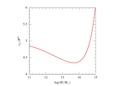
Figure 1: Mean separation between the protohalo and main mass fluctuation responsible for the tidal torque, scaled to the protohalo radius, as a function of the virial mass of the final halo (independent of the redshift, for virial masses) in the Planck14 cosmology.

After performing the integral (45) with such a value of $r_{\rm st}$, we arrive at the following mean Lagrangian protohalo AM

$$J^{\rm L}\approx\frac{4.95\times 10^{-3}}{\widetilde{m}+3}G\bar{\rho}^{1/3}_{0}\!\left(\frac{r_{\rm st}}{R^{\rm th}}\right)^{\widetilde{m}}[g(\gamma,\gamma\nu)M]^{5/3}\frac{\delta}{D(t_{\rm i})}.$$ (48)

In Figure 2 we plot $J^{\rm L}$ as a function of the virial mass $M$ of halos (regardless of $t_{0}$).

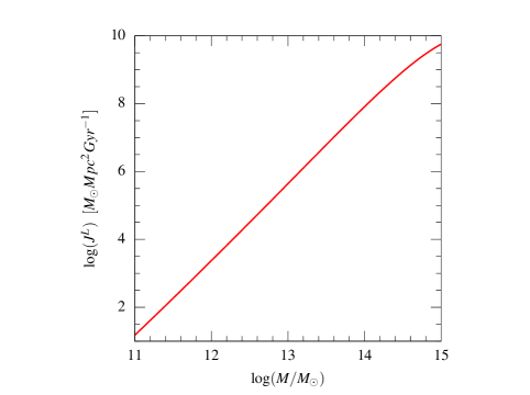
Figure 2: Mean Lagrangian protohalo AM as a function of the virial mass of the final halo in the Planck14 cosmology.

Similarly, by integrating $J^{\rm L}$ (eq. [45]) from $R^{\rm th}$ to the median distance $r_{\rm med}$ to the main tidal torque source solution of the equation

$$0.5=\frac{\int_{0}^{r_{\rm med}}{\rm d}r\,r^{\widetilde{m}+2}}{\int_{0}^{r_{\rm st}}{\rm d}r\,r^{\widetilde{m}+2}}=\left(\frac{r_{\rm med}}{r_{\rm st}}\right)^{\widetilde{m}+3}$$ (49)

implying $r_{\rm med}=r_{\rm st}/2^{1/(\widetilde{m}+3)}$, we are led to a median Lagrangian protohalo AM equal to $J^{\rm L}_{\rm med}=J^{\rm L}/2$.

5 Summary and Discussion

We have applied the TTT to derive the Lagrangian AM of protohaloes centred in Gaussian triaxial peaks in CDM cosmologies, accounting for their accurate extension (mass) and ellipsoidal collapse time. These improvements have been possible thanks to the use of the CUSP formalism, making the link between haloes with $M$ at $t$ and Gaussian peaks with density contrast $\delta$ on scale $R$ in the smoothed linear Gaussian random density field at an initial time $t_{\rm i}$.

The approach we have followed is innovative in the sense that not only is the protohalo a peak, but also the mass excess or defect responsible for the main tidal torque is a peak or a hole. Specifically, this mass fluctuation is found to be the largest peak or hole fitting in the neighbourhood of the protohalo (i.e. with top-hat scale $R^{\rm th}_{\rm d}$ equal to the separation $r_{\rm st}$) over the continuous $\delta(R)$ peak (or hole) trajectory starting as a twin (positive or negative) peak to that associated with the protohalo. Of course, there are many more positive and negative density fluctuations outside that trajectory in the neighbourhood of the protohalo that cause small additional tidal torques. However, these perturbations are very numerous and typically half of them slightly boosts the tidal torque caused by the main source and the other half mitigates it as they point to the opposite direction, so their global effect basically cancels.

The predicted mean Lagrangian AM of protohaloes with virial mass $M$ collapsing at $t_{\rm c}$, $J^{\rm L}(M,t_{\rm c})$ is analytic, so it can be readily checked against simulations and implemented in analytic models of structure formation. Its expression is

$$J^{\rm L}(M,t_{\rm c})\approx\frac{5.0\times 10^{-3}}{\widetilde{m}+3}G\bar{\rho}^{1/3}_{0}s^{\widetilde{m}}(M)\widetilde{M}^{5/3}\frac{\delta(t_{\rm c},t_{\rm i})}{D(t_{\rm i})},$$ (50)

where $\widetilde{m}=-13[(n+3)/2]/3\approx-2.71$ (for the CDM spectral index $n\approx-1.75$ corresponding to galactic haloes), $\bar{\rho}_{0}$ is the present mean cosmic density, $s$ is the time-invariant typical separation between the c.o.m. of the protohalo and the main tidal torque source scaled to the protohalo size, $s=r_{\rm st}/R^{\rm th}$ (eq. [47]), $\widetilde{M}\equiv g(\gamma,\gamma\nu)M$, where $g$ is given by equation (44), and $\delta(t_{\rm c},t_{\rm i})$, proportional to the cosmic growth factor at $D(t_{\rm i})$ (eq. [2]), is the density contrast of Gaussian peaks at $t_{\rm i}$ that collapse ellipsoidally at $t_{\rm c}$. On the other hand, the median Lagrangian protohalo AM is $J^{\rm L}(M,t_{\rm c})/2$. Both Lagrangian AMs are, of course, independent of the (arbitrary) initial time $t_{\rm i}$ and of the cosmic time $t$ as well, their Eulerian counterparts being multiplied by $a^{2}(t)\dot{D}(t)$.

On the contrary, $J^{\rm L}$ depends on $t_{\rm c}$ through $\delta(t_{\rm c},t_{\rm i})/D(t_{\rm i})$, and on the $M$ through the factor $M^{5/3}$, as found in simulations (e.g. Sugerman, Summers & Kamionkowski 2000) apart from the slight dependence arising from typical separation between the protohalo and the main source of the tidal source, $s(M)$, which stays around $4.5$ except at the high-mass end where the halo number density rapidly falls off and $s(M)$ goes to infinity, and from the very smooth factor $g(\gamma,\gamma\nu)$ arising from the triaxial shape and relative orientation of both objects.

No need to say that the Lagrangian protohalo AM derived here only holds in linear (and moderately non-linear) regime. However, in Paper II we use this result to infer the typical AM and spin of virialised haloes as well as their specific AM profile with unprecedented accuracy.

ACKNOWLEDGEMENTS

This work was funded by the Spanish MCIN/AEI/ 10.13039/501100011033 through grants CEX2019-000918-M (Unidad de Excelencia ‘María de Maeztu’, ICCUB) and PID2022-140871NB-C22 (co-funded by FEDER funds) and by the Catalan DEC through the grant 2021SGR00679.

DATA AVAILABILITY

The data underlying this article will be shared on reasonable request to the corresponding author.

Appendix A Tidal Tensor

The Hessian of the Lagrangian gravitational potential (36) is

$${\bf T}_{{\rm n}ij}\!\equiv\!\frac{a^{3}(t_{\rm i})}{D(t_{\rm i})}\frac{\partial^{2}\Phi_{\rm d}}{\partial x_{j}\partial x_{i}}\!=\!\frac{a^{3}(t_{\rm i})}{D(t_{\rm i})}\frac{4\pi\Delta[S({\bf 0})]}{\Delta[S({\bf x})]}G\delta_{\rm d}\bar{\rho}(t_{\rm i})\!\!\left(\!\frac{x_{i}x_{j}}{[a_{{\rm n}i}^{2}\!+\!S({\bf x})][a_{{\rm n}j}^{2}\!+\!S({\bf x})]}\!\left\{\sum_{k=1}^{3}\!\frac{x_{k}^{2}}{[a_{{\rm n}k}^{2}+S(\bf x)]^{2}}\!\right\}^{\!\!-1}\!\!\!\!-\delta_{ij}\!\int_{S({\bf x})}^{\infty}\!\!\frac{\Delta[S({\bf x})]\,{\rm d}s}{\Delta(s)(a^{2}_{{\rm n}i}\!+\!s)}\!\right)\!,$$ (51)

where $\delta_{ij}$ is the Kronecker delta, $\Delta[S({\bf x})]$ is given by equation (37) but with $s$ replaced by $S({\bf x})$ defined in equation (38).

Since $R_{\rm d}$ is limited by the condition $R_{\rm d}^{\rm th}=r$, the c.o.m. of the protohalo is at the edge of the ellipsoidal mass excess, i.e. $\sum_{k=1}^{3}x_{k}^{2}/a^{2}_{{\rm n}k}=1$ and $S({\bf x})=0$. Consequently, the tidal tensor is simply

$${\bf T}_{{\rm n}ij}=\frac{a^{3}(t_{\rm i})}{D(t_{\rm i})}4\pi G\delta_{\rm d}\bar{\rho}(t_{\rm i})\left[\frac{x_{i}x_{j}}{a^{2}_{{\rm n}i}a^{2}_{{\rm n}j}}\left(\sum_{k=1}^{3}\frac{x_{k}^{2}}{a_{{\rm n}k}^{4}}\right)^{\!-1}-\delta_{ij}U(a^{2}_{{\rm n}k})\right]\!,$$ (52)

where

$$U(a^{2}_{{\rm n}k})\equiv\frac{1}{2}\int_{0}^{\infty}\frac{{\rm d}s/a^{2}_{{\rm n}j}}{1+s/a_{{\rm n}j}^{2}}\left[\prod_{k=1}^{3}\left(1+\frac{s}{a^{2}_{{\rm n}k}}\right)\right]^{-1/2}=\frac{1}{2}\int_{1}^{\infty}\,\frac{{\rm d}y}{y^{3/2}}\left[\sum_{k=1}^{3}\frac{a_{{\rm n}j}+s(y)^{2}}{a_{{\rm n}k}^{2}+s(y)}\right]^{-1}.$$ (53)

Taking into account that the ellipticity and prolateness of peaks is moderate (BBKS), we have $U(a^{2}_{{\rm n}k})\approx\frac{1}{6}\int_{1}^{\infty}\,\frac{{\rm d}y}{y^{3/2}}=\frac{1}{3}$. In addition, we can neglect the terms in $1-a^{2}_{{\rm n}k}/a^{2}_{\rm d}$, where $a_{\rm d}^{2}\equiv 1/3\sum_{k=1}^{3}a^{2}_{{\rm n}k}$, in the Taylor expansion of $\sum_{k=1}^{3}x_{k}^{2}/a^{4}_{{\rm n}k}$ at $\sum_{k=1}^{3}x_{k}^{2}/(a^{2}_{{\rm n}k}a^{2}_{\rm d})$,

$$\sum_{k=1}^{3}\frac{x_{k}^{2}}{a_{{\rm n}k}^{4}}=\sum_{k=1}^{3}\frac{x_{k}^{2}}{a_{{\rm n}k}^{2}a_{\rm d}^{2}}\left[1+\left(1-\frac{a_{{\rm n}k}^{2}}{a^{2}_{\rm d}}\right)+...\right]\approx\frac{1}{a_{\rm d}^{2}}\sum_{k=1}^{3}\frac{x_{k}^{2}}{a_{{\rm n}k}^{2}}=\frac{1}{a_{\rm d}^{2}}.$$ (54)

Thus we arrive at the almost fully accurate expression

$${\bf T}_{{\rm n}ij}=\frac{a^{3}(t_{\rm i})}{D(t_{\rm i})}\frac{4\pi}{3}G\delta_{\rm d}\bar{\rho}(t_{\rm i})\left[3\frac{x_{i}x_{j}}{a^{2}_{{\rm n}i}a^{2}_{{\rm n}j}}a_{\rm d}^{2}-\delta_{ij}\right].$$ (55)

Note that in the limit $a_{{\rm n}k}=R^{\rm th}_{\rm d}$, where the two approximations above hold exactly, expression (55) recovers the Hessian of the gravitational potential at the edge ($r=R_{\rm d}^{\rm th}$) of a spherically symmetric system, as expected.

Appendix B Orientation Averages

As argued in Section 4, to find the modulus of the Lagrangian AM of a protohalo we must simply perform the average of any arbitrary component, e.g. for $i=1$, of such an AM, equation (40), over the two sets of Euler angles giving the orientation of the protohalo and of the ellipsoidal mass excess. To do that average we adopt the simplest initial configuration of the system, i.e. that in which the principal axes of both objects are aligned with each other though with different indexes in general (see below for the interest of that freedom) and with the position vector ${\bf r}$ of the centre of the protohalo from that of the mass excess.

Since the averages over the two sets of Euler angles may be carried out independently, we can start by averaging over $\alpha$, $\beta$ and $\kappa$ in the whole angular space $8\pi^{2}$ strad². The scaled inertia tensor (eq. [20]) then becomes

$$\langle{\bf I}\rangle_{\alpha,\beta,\kappa}=\frac{M}{15a^{2}(t_{\rm i})}\left(\begin{matrix}\iota_{1}&0&0\\ 0&\iota_{2}&0\\ 0&0&\iota_{3}\end{matrix}\right),$$ (56)

of the component $i$ of the AM reads

$$\langle J^{\rm L}_{{\rm n}i}\rangle_{\alpha,\beta,\kappa}=-\frac{M}{15a^{2}(t_{\rm i})}\epsilon_{ijk}\,[{\bf R_{\rm d}T_{\rm d}R_{\rm d}^{\!T}}]_{jk}\iota_{k}.$$ (57)

or, equivalently,

$$\langle J^{\rm L}_{{\rm n}i}\rangle_{\alpha,\beta,\kappa}=-\frac{M}{15a^{2}(t_{\rm i})}[{\bf R_{\rm d}T_{\rm d}R_{\rm d}^{\!T}}]_{jk}\left(\iota_{j}-\iota_{k}\right),$$ (58)

with $i$, $j$ and $k$ following the natural (ciclic) order.

As mentioned, the principal axes of I may not coincide with those of ${\bf T_{\rm d}}$. Thus, regardless of the orientation of T, we may assume $\iota_{j}-\iota_{k}\equiv a_{k}^{2}-a_{j}^{2}$ in equation (57) equal to $a_{3}^{2}-a_{1}^{2}$. This is very convenient because we simply have (see eqs. [18]-[19])

$$a_{3}^{2}-a_{1}^{2}=\frac{1}{a_{3}^{-2}}-\frac{1}{a_{1}^{-2}}=\frac{a_{1}^{-2}-a_{3}^{-2}}{a_{3}^{-2}a_{1}^{-2}}=\frac{\hat{a}_{1}^{-2}-\hat{a}_{3}^{-2}}{\hat{a}_{3}^{-2}\hat{a}_{1}^{-2}}=2p\left[\frac{(1-2e)^{2}}{(1+e)^{2}-9p^{2}}\right]^{1/3}\approx 2\left(\frac{1-2e}{3}\right)^{2/3}p^{1/3},$$ (59)

where we have neglected $|(1+e)/(3p)|$ in front of unity (not only is $|p|\leq e$, but, for peaks of galaxy mass, $|p|\ll 1$).

Consequently, we have

$$\langle J^{\rm L}_{{\rm n}i}\rangle_{\alpha,\beta,\kappa}\approx\frac{2}{3^{2/3}}\frac{M(R^{\rm th})^{2}}{15a^{2}(t_{\rm i})}[{\bf R_{\rm d}T_{\rm d}R_{\rm d}^{\!T}}]_{jk}\,\left(1-2e\right)^{2/3}p^{1/3}.$$ (60)

in terms of the ellipticity and prolateness of the peak associated with the protohalo.

We must now average over the Euler angles $\alpha_{\rm d}$, $\beta_{\rm d}$ and $\kappa_{\rm d}$ in $8\pi^{2}/2$ strad² from any arbitrary initial orientation of the position vector ${\bf r}_{\rm d}$ of the c.o.m. of the protohalo (e.g. in the $a_{{\rm n}i}$ direction). We remark that, even though the top-hat scale $R_{\rm d}^{\rm th}$ of the ellipsoidal mass excess was chosen to be bounded to $r$ so that we must not worry about possible outer shells not contributing to the tidal force, when $R^{\rm th}_{\rm d}$ is close to $r$, the c.o.m. of the protohalo may be found inside or outside the ellipsoidal mass excess depending on the orientation of ${\bf r}_{\rm d}$. Consequently, in these circumstances, the average over the Euler angles $\alpha_{\rm d}$, $\beta_{\rm d}$ and $\gamma_{\rm d}$ will slightly overestimate the real AM of the protohalo when the peak lies inside the ellipsoidal mass excess or slightly underestimate it otherwise because the scale of the real ellipsoidal mass excess responsible of the torque could have been taken somewhat larger. Both effects should essentially balance, however, so we can forget about that complication and keep the tidal tensor with the form (57) regardless of the orientation. On the other hand, for the reasons mentioned in Section 4 we can concentrate in the orientation average over $4\pi^{2}$ strad² only of any particular component, e.g. component 1, of the AM vector.

After a lengthy calculation, we arrive at the following average over $\alpha_{\rm d}$, $\beta_{\rm d}$ and $\kappa_{\rm d}$ in $4\pi^{2}$ strad² of $[{\bf R_{\rm d}T_{\rm d}R_{\rm d}^{\!T}}]_{23}$ with ${\bf T_{\rm d}}$ given by equation (55)

$$\langle[{\bf R_{\rm d}T_{\rm d}R_{\rm d}^{\!T}}]_{23}\rangle_{\alpha_{\rm d},\beta_{\rm d},\kappa_{\rm d}}=\frac{a^{3}(t_{\rm i})G\bar{\rho}(t_{\rm i})\delta}{3D(t_{\rm i})}\left(\frac{r}{R^{\rm th}}\right)^{m}H\!\left(a_{{\rm n}i}\right)$$ (61)

$$H(a_{{\rm n}i})\!\equiv\!\frac{4\pi-9}{36}\!+\!a_{\rm d}^{2}\frac{\langle x_{\rm d}\rangle}{\Lambda_{\rm d}}\!\left\{\frac{5\pi-8}{30}\hat{a}_{{\rm n}1}^{-4}\!+\!\left(\!\frac{8}{9\pi}+\frac{26+75\pi}{120}\!\right)\!\hat{a}_{{\rm n}1}^{-2}\hat{a}_{{\rm n}2}^{-2}\!-\!\frac{1}{10}\hat{a}_{{\rm n}2}^{-4}\!-\!\frac{1}{5}\hat{a}_{{\rm n}1}^{-2}\hat{a}_{{\rm n}3}^{-3}\!-\!\left(\!\frac{1}{5\pi}+\frac{3\pi}{16}\!\right)\!\hat{a}_{{\rm n}2}^{-2}\hat{a}_{{\rm n}3}^{-2}\!+\!\frac{4}{5}\hat{a}_{{\rm n}3}^{-4}\right\}\!,$$ (62)

where we have have taken into account the equality $\delta_{\rm d}=(R_{\rm d}/R)^{m}\delta$ with $m=-[(n+3)/2]^{1/2}$ and $R_{\rm d}/R=r/R^{\rm th}$. Taking into account the equality $\hat{a}_{{\rm n}i}^{-2}=\lambda_{{\rm n}i}/\langle x_{\rm d}\rangle$, $H$ adopts the following approximate form as a function of $e_{\rm d}$ (or $\tilde{e}_{\rm d}=-(1-2e_{\rm d})/3$) and $p_{\rm d}$

$$10H(e_{\rm d},p_{\rm d})\!\approx\!1\!+\!\frac{p_{\rm d}^{-2/3}}{3}\!\left(\!\tilde{e}_{\rm d}^{2/3}\!+\!\tilde{e}_{\rm d}^{8/3}\!-\!\tilde{e}_{\rm d}^{14/3}\!\right)\!\left\{\!1\!+\!\frac{0.6p_{\rm d}\tilde{e}_{\rm d}^{-1}}{1\!+\!\tilde{e}_{\rm d}}\!\left[90\!-\!\left(\frac{1}{\tilde{e}_{\rm d}}\!-\!2\right)^{\!3}\right]\!\right\}\!\approx\!1\!+\!\frac{p_{\rm d}^{-2/3}}{3}\!\left(\!\tilde{e}_{\rm d}^{2/3}\!+\!\tilde{e}_{\rm d}^{8/3}\!-\!\tilde{e}_{\rm d}^{14/3}\right)\!\left(\!1+\!\frac{54p_{\rm d}\tilde{e}_{\rm d}^{-1}}{1+\tilde{e}_{\rm d}}\!\right)\!.$$ (63)

Taking into account that $\tilde{e}_{\rm d}\la 0.3$, $H(e_{\rm d},p_{\rm d})$ can be further approximated to

$$10H(e_{\rm d},p_{\rm d})\approx 1+(\tilde{e}_{\rm d}p_{\rm d})^{-1/3}\left[16+\frac{1}{3p_{\rm d}^{4/3}}(\tilde{e}_{\rm d}p_{\rm d})\right]=1-3^{1/3}[(1-2e_{\rm d})p_{\rm d}]^{-1/3}\left[16-3^{-2}(1-2e_{\rm d})p_{\rm d}^{-1/3}\right]$$ (64)

Having performed those two averages, the typical value of e.g. the first Cartesian component of the Lagrangian proptohalo AM takes the form

$$J^{\rm L}_{{\rm n}1}\equiv\langle\langle J^{\rm L}_{{\rm n}1}\rangle_{\alpha,\beta,\kappa}\rangle_{\alpha_{\rm d},\beta_{\rm d},\kappa_{\rm d}}\approx\frac{2}{3^{5/3}}\frac{G\bar{\rho}^{1/3}_{0}\delta\,M^{5/3}}{5D(t_{\rm i})}\left(\frac{r}{R^{\rm th}}\right)^{m}H\!\left(e_{\rm d},p_{\rm d}\right)\left(1-2e\right)^{2/3}p^{1/3},$$ (65)

where $\bar{\rho}_{0}$ is the current mean cosmic density, implying an average modulus of the Lagrangian AM equal to

$$J^{\rm L}_{\rm d}=\sqrt{3}J^{\rm L}_{{\rm n}i}\approx\frac{2}{5\times 3^{7/6}D(t_{\rm i})}G\bar{\rho}^{1/3}_{0}\delta\,M^{5/3}\left(\frac{r}{R^{\rm th}}\right)^{m}\,H\!\left(e_{\rm d},p_{\rm d}\right)(1-2e)^{2/3}p^{1/3}.$$ (66)

Appendix C Ellipticity and prolateness average

We must average $J^{\rm L}_{\rm d}$ given by equation (66) over the ellipticity and prolateness of the peaks associated with the protohalo and the dominant mass excess causing the torque.

Taking into account the following approximate averages of powers of $p$ from $-e$ to $e$ holding for massive haloes, with $e\la 0.3$ and $p\ll\sigma_{p}$,

$$\overline{p^{1/3}}(e)\approx\frac{6e^{4/3}}{\sqrt{2\pi}\sigma_{p}}\,{\rm e}^{-\frac{\bar{p}^{2}}{2\sigma_{p}^{2}}}\left[\frac{e\bar{p}}{7\sigma_{p}^{2}}+O(e^{3})\right]\approx\frac{6e^{7/3}\bar{p}}{7\sqrt{2\pi}\sigma_{p}^{3}}$$ (67)

$$\overline{p^{-1/3}}(e)\approx\frac{6e^{2/3}}{\sqrt{2\pi}\sigma_{p}}\,{\rm e}^{-\frac{\bar{p}^{2}}{2\sigma_{p}^{2}}}\left[\frac{e\bar{p}}{5\sigma_{p}^{2}}+O(e^{3})\right]\approx\frac{6e^{5/3}\bar{p}}{5\sqrt{2\pi}\sigma_{p}^{3}}$$ (68)

$$\overline{p^{-2/3}}(e)\approx\frac{6e^{1/3}}{\sqrt{2\pi}\sigma_{p}}{\rm e}^{-\frac{\bar{p}^{2}}{2\sigma_{p}^{2}}}\left[1-\frac{e^{2}(\bar{p}^{2}-\sigma_{p}^{2})}{14\sigma_{p}^{2}}+O(e^{3})\right]\approx\frac{6e^{1/3}}{\sqrt{2\pi}\sigma_{p}}\left[1+\frac{e^{2}}{14}\right],$$ (69)

the averages of $J^{\rm L}_{\rm d}$ over $p$ and $p_{\rm d}$ lead to

$$J^{\rm L}_{\rm d}\approx\frac{4}{35\times 3^{1/6}\sqrt{2\pi}}\frac{G\bar{\rho}^{1/3}_{0}\delta\,M^{5/3}}{D(t_{\rm i})}\left(\frac{r}{R^{\rm th}}\right)^{m}\,H(e_{\rm d})\frac{e^{7/3}(1-2e)^{2/3}\bar{p}}{\sigma_{p}^{3}}\,{\rm e}^{-\frac{\bar{p}^{2}}{2\sigma_{p}^{2}}},$$ (70)

where

$$10H(e_{\rm d})\approx 1-\frac{24\times 3^{4/3}}{5\sqrt{2\pi}\sigma_{p}^{3}}(1-2e_{\rm d})^{-1/3}e_{\rm d}^{5/3}\bar{p}_{\rm d}{\rm e}^{-\frac{\bar{p}_{\rm d}^{2}}{2\sigma^{2}_{{\rm n}p}}}+\frac{2\times 3^{-2/3}}{\sqrt{2\pi}\sigma_{p}}(1-2e_{\rm d})^{-2/3}e_{\rm d}^{1/3}\left[1+\frac{e_{\rm d}^{2}}{14}\right]{\rm e}^{-\frac{\bar{p}_{\rm d}^{2}}{2\sigma^{2}_{{\rm n}p}}},$$ (71)

where $\bar{p}$ and $\bar{p}_{\rm d}$ are much smaller than unity, $e$ and $e_{\rm d}$ are smaller than unity and $O(\sigma_{p})=O(\sigma_{e})=O(\bar{e})$. Thus, to leading order in all those small quantities we have

$$J^{\rm L}_{\rm d}\approx\frac{4}{35\times 3^{1/6}\sqrt{2\pi}}\frac{G\bar{\rho}^{1/3}_{0}\delta\,M^{5/3}}{D(t_{\rm i})}\left(\frac{r}{R^{\rm th}}\right)^{m}\,H(e_{\rm d})\frac{e^{7/3}\bar{p}}{\sigma_{p}^{3}},$$ (72)

$$10H(e_{\rm d})\approx 1+\frac{2\times 3^{-2/3}}{\sqrt{2\pi}\sigma_{{\rm n}p}}\,e_{\rm d}^{1/3}.$$ (73)

And, taking into account the following approximate averages of powers of $e$ from $-(\bar{e}+3\sigma_{e})=-1.40\bar{e}$ to $(\bar{e}+3\sigma_{e})=1.40\bar{e}$ (even though $e$ is positive, it is convenient to extend the integral to negative $e$ values, as done to find the normalisation constant of the PDF)

$$\overline{e^{1/3}}=\frac{6}{\sqrt{2\pi}\sigma_{e}}(1.4\bar{e})^{4/3}{\rm e}^{-\frac{\bar{e}^{2}}{2\sigma_{e}^{2}}}\left[\frac{(1.4\bar{e})}{7}\frac{\bar{e}}{\sigma_{e}^{2}}+O(\bar{e}^{3})\right]\approx\frac{6\times 1.4^{7/3}}{7{\rm e}^{3}\sqrt{2\pi}}\frac{\bar{e}^{7/3}}{\sigma_{e}^{3}}$$ (74)

$$\overline{e^{7/3}}=\frac{6}{\sqrt{2\pi}\sigma_{e}}(1.4\bar{e})^{10/3}{\rm e}^{-\frac{\bar{e}^{2}}{2\sigma_{e}^{2}}}\left[\frac{(1.4\bar{e})}{13}\frac{\bar{e}}{\sigma_{e}^{2}}+O(\bar{e}^{3})\right]\approx\frac{6\times 1.4^{13/3}}{13{\rm e}^{3}\sqrt{2\pi}}\frac{\bar{e}^{10/3}}{\sigma_{e}^{3}}$$ (75)

and the equalities $\sigma_{e}=e/\sqrt{6}$ and $\sigma_{p}=e/\sqrt{3}$, we find, to leading order, the following average over $e$ and $e_{\rm d}$

$$J^{\rm L}_{\rm d}\approx 5.5\times 10^{-4}\,\frac{G\bar{\rho}^{1/3}_{0}\delta\,M^{5/3}}{D(t_{\rm i})}\left(\frac{r}{R^{\rm th}}\right)^{m}\bar{e}^{-10/3}_{\rm d}\bar{e}^{-2/3}\bar{p}=3.3\times 10^{-3}\,\frac{G\bar{\rho}^{1/3}_{0}\delta\,M^{5/3}}{D(t_{\rm i})}\left(\frac{r}{R^{\rm th}}\right)^{m}\left(\frac{\bar{e}}{\bar{e}_{\rm d}}\right)^{10/3}.$$ (76)

Lastly, expressing $\bar{e}$ and $\bar{e}_{\rm d}$ as functions of $\langle x\rangle$ and $\langle x_{\rm d}\rangle$ (see the comment on eq. [12]) and, taking into account that for large masses, as it is the case for the dominant mass excess, the average curvature $\langle x_{\rm d}\rangle$ is $\approx\gamma\nu_{\rm d}=(r/R^{\rm th})^{m}\gamma\nu$, where $r/R^{\rm th}\gg 1$, and adopting $M_{\rm vir}$ masses so that $R_{\rm d}/R\approx r/R^{\rm th}$, we obtain

$$J^{\rm L}_{\rm d}\approx 3.3\times 10^{-3}\,\frac{G\bar{\rho}^{1/3}_{0}\delta\,M^{5/3}}{D(t_{\rm i})}\left(\frac{r}{R^{\rm th}}\right)^{\widetilde{m}}\left[\frac{(\gamma\nu)^{2}}{\langle x\rangle^{2}+\frac{6}{5}}\right]^{5/3},$$ (77)

where $\widetilde{m}=13m/3$.

References

- Abdullah et al. (2024) Abdullah M. H., Klypin A., Prada F., Wilson G., Ishiyama T., Ereza J., 2024, MNRAS, 529, L545
- Bardeen et al. (1986) Bardeen J. M., Bond J. R., Kaiser N., Szalay A. S., 1986, ApJ, 304, 15 (BBKS)
- Bond et al. (1991) Bond, J.R., Cole, S., Efstathiou, G., & Kaiser, N. 1991, ApJ, 379, 440
- Bryan & Norman (1998) Bryan G.L. & Norman M. L., 1998, ApJ, 495, 80
- Catelan & Theuns (1996a) Catelan P., Theuns T., 1996a, MNRAS, 282, 436
- Catelan & Theuns (1996b) Catelan P., Theuns T., 1996b, MNRAS, 282, 455
- Chandrasekhar (1987) Chandrasekhar S., 1987, efe..book
- Doroshkevich (1970) Doroshkevich, A. G. 1970, Astrophysics, 6, 320
- Henry (2000) Henry, J. P., 2000, ApJ, 534, 565
- Hoffman (1988) Hoffman Y., 1988, ApJ, 329, 8
- Hoyle et al. (1949) Hoyle F., Burgers J. M., van de Hulst H. C., 1949, eds., in Problems of Cosmical Aerodynamics, Central Air Documents Office, Dayton, p. 195
- Juan et al. (2014) Juan E., Salvador-Solé E., Domènec G., Manrique A., 2014, MNRAS, 439, 719
- Komatsu et al. (2011) Komatsu E., Smith K. M., Dunkley J., Bennett C. L., Gold B., Hinshaw G., Jarosik N., et al., 2011, ApJS, 192, 18L137
- Manrique & Salvador-Solé (1995) Manrique A. & Salvador-Solé E., 1995, ApJ, 453, 6
- Manrique & Salvador-Solé (1996) Manrique A. & Salvador-Solé E., 1996, ApJ, 467, 504
- Manrique et al. (1998) Manrique A., Raig A., Solanes J. M., González-Casado G., Stein, P., Salvador-Solé E., 1998, ApJ, 499, 548
- Heavens & Peacock (1988) Heavens A., Peacock J., 1988, MNRAS, 232, 339
- Peebles (1969) Peebles P. J. E., 1969, ApJ, 155, 393
- Planck Collaboration et al. (2014) Planck Collaboration, Ade, P. A. R., Aghanim, N., et al. 2014, A&A, 571, AA16
- Porciani, Dekel, & Hoffman (2002a) Porciani C., Dekel A., Hoffman Y., 2002a, MNRAS, 332, 325
- Porciani, Dekel, & Hoffman (2002b) Porciani C., Dekel A., Hoffman Y., 2002, MNRAS, 332, 339
- Salvador-Solé & Manrique (2021) Salvador-Solé E., Manrique A., 2021, ApJ, 914,141
- Salvador-Solé & Manrique (2024) Salvador-Solé E., Manrique A., 2024, accepted for publication in ApJ
- Salvador-Solé, Manrique & Agulló (2024) Salvador-Solé E., Manrique A., Agulló E., 2024, submitted to ApJ
- Sugerman, Summers & Kamionkowski (2000) Sugerman B., Summers F. J., Kamionkowski M., 2000, MNRAS, 311, 762
- Thuan & Gott (1977) Thuan T. X., Gott J. R., 1977, ApJ, 216, 194
- White (1984) White, S. D. M. 1984, ApJ, 286, 38