ORIGIN AND FULL CHARACTERIZATION OF THE SECONDARY (ASSEMBLY) HALO BIAS

Abstract

Not only are halos of different masses differently clustered, the so-called primary bias, but halos with distinct internal properties also are, which is known as secondary bias. Contrarily to the former bias, the latter is not understood within the Press-Schechter (PS) and excursion set (ES) formalisms of structure formation, where protohalos are fully characterised by their height and scale. As halos in different backgrounds undergo mergers at different rates, the secondary bias was suggested not to be innate but to arise from the distinct assembly history of halos. However, it has recently been proven that mergers leave no imprint in halo properties. But, in the peak model of structure formation, the secondary bias could still be innate and arise from the different typical curvature of peaks lying in different backgrounds. Here we show that this is the case, indeed. Using the CUSP formalism, we find that peaks lying in different backgrounds with different typical curvatures evolve in halos with different density profiles which in turn lead to many other distinct properties. The dependence we find of halo bias with those properties reproduces the results of simulations.

1 INTRODUCTION

One fundamental property of the Universe is that light does not trace matter. Massive galaxies are more clustered than less massive ones (Capelato et al., 1980) and galaxies of a given mass but different mass-to-light ratios, morphologies or star formation rates are also differently clustered (Faber & Gallagher, 1979; Dressler, 1980; Poggianti et al., 1999). As the spatial distribution of cosmic objects informs on their formation and evolution, the discovery of those segregations gave rise to a lively “nature vs. nurture” debate (Sanromà & Salvador-Solé, 1990; Dressler et al., 1997; Ellis et al., 1997; Smith et al., 2005). In fact, galaxies form and develop within dark matter (DM) halos, which are themselves segregated (biased) in mass as well as in other internal properties, so the properties of galaxies are tightly coupled to those of halos and their substructure (e.g. Peacock & Smith 2000; Seljak 2000; Zentner et al. 2005; Montero-Dorta et al. 2020; Xu & Zheng 2020).

It is now well-established that the mass segregation of halos (Hauser & Peebles, 1973; Bahcall & Soneira, 1983), the so-called primary bias, is already imprinted in the primordial density field (Kaiser 1984; Bardeen et al. 1986, hereafter BBKS). However, the reason why halos with the same mass but different internal properties are also differently clustered, the so-called secondary bias, is poorly understood.

The first evidence in simulations of the secondary bias was found by Sheth & Tormen (2004) who noticed that halos in pairs form earlier than more isolated ones. Harker et al. (2006) showed that, in general, the more strongly clustered halos, the smaller their formation time, an effect which was confirmed by other authors (Gao, Springel, & White, 2005; Harker et al., 2006; Zhu et al., 2006; Wechsler et al., 2006; Wetzel et al., 2007; Jing, Suto, & Mo, 2007). In addition, Wechsler et al. (2006) found that low-mass halos with the higher concentration are more clustered and the opposite is true for high-mass halos. Lastly, Gao & White (2007) showed that the secondary bias affects other halo properties such as the peak velocity, subhalo abundance (or halo occupation number) and spin. Those trends were subsequently confirmed and extended to other properties such as velocity anisotropy and shape (Macciò et al. 2007; Angulo, Baugh, & Lacey 2008; Faltenbacher & White 2010; Lee et al. 2017; Mao, Zentner & Wechsler 2018; Sato-Polito et al. 2019; Chen et al. 2020; Lazeyras et al. 2023; see also Hahn et al. 2009; Ramakrishnan & Paranjape 2020; Montero-Dorta et al. 2020; Hellwing et al. 2021).

In the PS (Press & Schechter, 1974) and excursion set (ES; Bond et al. 1991) models of structure formation, using top-hat and $k$-sharp smoothing windows, respectively, protohalos are fully characterized by their height and scale, which determine the mass and collapse time of halos regardless of their environment, so there is no room for halos of a given mass at a given time to have distinct internal properties according to their background (Gao & White, 2007). Since simulations also show that the merger history of halos depends on their environment (Gottlöber, Klypin, & Kravtsov, 2001; Gottlöber et al., 2002; Fakhouri & Ma, 2009, 2010; Wetzel et al., 2007), the idea came out that the secondary bias could be the result of the distinct assembly (merging) history of halos with identical seeds but evolving in different environments. This is why the secondary bias was also called “assembly bias”. However, neither the different merger rate or collapse time of halos evolving in different environments nor other evolutionary mechanisms explored (Mo et al., 2005; Sandvik et al., 2007; Desjacques, 2008; Hahn et al., 2009; Yu et al., 2017) could reproduce the observed properties of the secondary bias.

Furthermore, numerical experiments (Moore et al. 1999; Huss et al. 1999; Hansen et al. 2006; Wang & White 2009; Barber et al. 2012; but see Hester & Tasitsiomi 2010; Wang et al. 2020) showed that mergers leave no imprint in halo properties (except in their substructure). The result found by Wang & White (2009) is particularly compelling in the context of the assembly bias: all internal properties of halos except subhalo abundance are identical in purely accreting halos (i.e. having undergone monolithic collapse) than in halos grown hierarchically (i.e. having suffered major mergers). In addition, Mao, Zentner & Wechsler (2018) and Chen et al. (2020) found that the secondary bias does not correlate with the assembly (or merger) history of halos. Last but not least, Salvador-Solé & Manrique (2021) have recently formally proven that fundamental result in structure formation.

But the possibility remains that a finer model of structure formation can account for the innate origin of the secondary bias. In fact, (Zentner, 2007) showed that the ES model with a filter different than the $k$-sharp one so that protohalos are sensitive to the matter distribution on larger scales leads to halos with formation times dependent on the background. Though that was a generic at general result which did not explain the details of simulations, it showed that an innate origin of the secondary bias was still possible.

Dalal et al. (2008) noted that, in the peak model where halos form from the collapse of patches around density maxima (peaks) in the smoothed linear Gaussian random density field, protohalos are characterised not only by their height at a given scale, but also by their curvature (i.e. minus the Laplacian of the density field at the peak scaled to its rms value) whose typical values depend on the peak background. Consequently, halos could have different internal properties and formation times arising in a simple natural manner from the specific properties of their seeds, regardless of their assembly history or other environmental effects.

Unfortunately, some difficulties met in the peak model (see Salvador-Solé & Manrique 2024a, hereafter Paper I) have so far prevented from checking this. If the derivation of the primary bias was already challenging, examining whether the secondary bias can be explained in that framework was even harder as it requires, in addition, connecting the curvature of peaks with the typical internal properties of halos. However, that is now feasible thanks to the ConflUent System of Peak trajectories (CUSP) formalism, that establishes such a connection from first principles and with no free parameter (Salvador-Solé & Manrique, 2021). In Paper I we applied CUSP to derive in a robust way the primary bias in the peak model. Here we use it to explain and characterize the secondary bias.

The layout of the Paper is as follows. In Section 2 we remind the basics of the CUSP formalism. In Section 3.2, we compare the average density profile of unconstrained halos to that of halos lying in a background predicted by CUSP. The consequences of this relation on the different internal properties of halos involved in the secondary bias are examined in Section 4. Our results are summarised and the main conclusions are drawn in Section 5.

2 Halo-Peak Correspondence

CUSP allows one to derive all macroscopic halo properties from peak statistics in the linear random Gaussian density field smoothed with a Gaussian filter. This is possible thanks to the fact that there is a one-to-one correspondence between halos with $M$ at $t$ (for any particular mass definition) and peaks with density contrast $\delta$ at the smoothing scale $R$ at the (arbitrary) initial time $t_{\rm i}$. The reader is referred to Salvador-Solé & Manrique (2021) for details. Next we provide a quick summary of this correspondence.

The time of ellipsoidal collapse $t$ of patches around peaks depends not only on their mass and size as in top-hat spherical collapse, but also on their triaxial shape and concentration (Peebles, 1969). Nonetheless, the probability distribution functions (PDFs) of ellipticities $e$, prolatenesses $p$, and curvatures $x$ of peaks with $\delta$ at scale $R$ are very sharply peaked (BBKS), so peaks with any given $\delta$ at $R$ have essentially the same fixed values of those quantities, implying that they collapse and virialize essentially at the same time $t$, dependent only on $\delta$ at a fixed scale. Consequently, given any mass definition of halos fixing their mass $M$ at $t$, the scale $R$ of the corresponding peaks with $\delta(t)$ at $t_{\rm i}$ define the relation between $R$ and $M$, dependent on $t$ in general, for peaks collapsing in halos with $M$ at $t$.

As shown by Juan et al. (2014a), the relations $\delta(t)$ and $R(M,t)$ can be found, for any given cosmology and halo mass definition, by enforcing the consistency conditions that i) at any time $t$ all the DM in the Universe is locked in halos of different masses and ii) the mass $M$ of a halo must be equal to the volume-integral of its density profile (see Sec. 3 for its derivation). Specifically, writing those two functions in the form

$$\delta(t,t_{\rm i})=r_{\delta}(t)\,\delta_{\rm c}^{\rm th}(t)\frac{D(t_{\rm i})}{D(t)}$$ (1)

$$\sigma_{0}(R,t,t_{\rm i})=r_{\sigma}(M,t)\,\sigma_{0}^{\rm th}(M,t)\frac{D(t_{\rm i})}{D(t)}\,,$$ (2)

where $\delta_{\rm c}^{\rm th}(t)$ is the linearly extrapolated density contrast for top-hat spherical collapse at $t$, $a(t)$ is the cosmic scale factor, $D(t)$ is the linear growth factor, $\sigma_{0}(R,t,t_{\rm i})$ is the Gaussian 0th-order spectral moment at $t_{\rm i}$ on the scale $R$ corresponding to the mass $M$ at $t$ and $\sigma_{0}^{\rm th}(M,t)$ is its top-hat counterpart at $t$, the functions $r_{\delta}$ and $r_{\sigma}$ appear to be well fitted in all cosmologies and halo mass definitions analysed by the analytic expressions

$$r_{\delta}(t)\approx\frac{a^{d{\cal D}(t)}(t)}{D(t)}\,~{}~{}~{}~{}~{}~{}~{}~{}~{}~{}~{}~{}~{}~{}~{}~{}~{}~{}~{}~{}~{}~{}~{}~{}~{}~{}~{}~{}~{}~{}~{}~{}~{}~{}~{}~{}~{}~{}~{}~{}~{}~{}~{}~{}~{}~{}~{}~{}~{}~{}$$

$${\cal D}(t)=1-d_{0}a^{0.435/a(t)}(t)\phantom{\frac{}{}}~{}~{}~{}~{}~{}~{}~{}~{}~{}~{}~{}~{}~{}~{}~{}~{}~{}~{}~{}~{}~{}~{}~{}~{}~{}~{}~{}~{}~{}~{}~{}~{}~{}~{}~{}~{}~{}~{}$$ (3)

$$r_{\sigma}(M,t)\approx 1+r_{\delta}(t){\cal S}(t)\nu^{\rm th}(M,t)~{}~{}~{}~{}~{}~{}~{}~{}~{}~{}~{}~{}~{}~{}~{}~{}~{}~{}~{}~{}~{}~{}~{}~{}~{}~{}~{}~{}~{}$$

$${\cal S}(t)=s_{0}\!+\!s_{1}a(t)\!+\!\log\left[\frac{a^{s_{2}}(t)}{1\!+\!a(t)/A}\right],~{}~{}~{}~{}~{}~{}~{}~{}~{}~{}~{}~{}~{}~{}~{}~{}~{}~{}~{}~{}~{}~{}~{}~{}$$ (4)

with $\nu^{\rm th}(M,t)\equiv\delta^{\rm th}(t,t_{\rm i})/\sigma^{\rm th}_{0}(M,t_{\rm i})=\delta^{\rm th}_{\rm c}(t)/\sigma^{\rm th}_{0}(M,t)$ equal to the peak height in top-hat spherical collapse. See Table 1 for the values of coefficients $d$, $s_{0}$, $s_{1}$, $s_{2}$, and $A$ for several cosmologies (Table 2) and halo mass definitions of interest. Note that while $R$ increases with increasing $M$, $\delta$ decreases with increasing $t$. We remark that the analytic fitting function $r_{\delta}(t)$ given by equation (3) only holds up to the present time; its extrapolation to larger times should be taken with caution (see Sec. 4). In the case of virial masses ($M_{\rm vir}$), $r_{\sigma}$ is a function of $M$ alone, $r_{\sigma}(M)=1+c/\sigma_{0}^{\rm th}(M)$, where $\sigma_{0}^{\rm th}(M)$ is the top-hat 0th order spectral moment at the present time and $c=0.14$ and 0.10 in the WMAP7 and Planck14 cosmologies, respectively (Paper I).

Table 1: Coefficients in the halo-peak relations.

Cosmol.​	​Mass${}^{*}\!$	$d$	$10d_{0}\!\!$	$10^{2}s_{0}\!\!$	$10^{2}s_{1}\!\!$	$10^{2}s_{2}\!\!$	$A$
WMAP7​	$M_{\rm vir}\!$	1.06	3.0	4.22	3.75	3.18	25.7
	$M_{200}\!$	1.06	3.0	1.48	6.30	1.32	12.4
Planck14​	$M_{\rm vir}\!$	0.93	0.0	2.26	6.10	1.56	11.7
	$M_{200}\!$	0.93	0.0	3.41	6.84	2.39	6.87

${}^{*}M_{\rm vir}$ and $M_{200}$ are the masses inside the region with a mean inner density equal to $\Delta_{\rm vir}(t)$ (Bryan & Norman, 1998) times the mean cosmic density and 200 times the critical cosmic density, respectively.

Table 2: Cosmological Parameters.

Cosmology	$\Omega_{\Lambda}$	$\Omega_{\rm m}$	$h$	$n_{\rm s}$	$\sigma_{8}$	$\Omega_{b}$
WMAP7a	0.73	0.27	0.70	0.95	0.81	0.045
Planck14b	0.68	0.32	0.67	0.96	0.83	0.049

^a Komatsu et al. (2011).
^b Planck Collaboration et al. (2014).

Strictly speaking, some peaks with $\delta$ at $R$ are nested into other peaks with the same $\delta$ at a larger scale, so they are actually captured by the more massive halo associated with the host peak before achieving full collapse and become subhalos instead of halos at $t$. Therefore, equations (1) and (2) do not define a one-to-one correspondence between halos and peaks. This means that the abundance of peaks with $\delta$ and $R$ at $t_{\rm i}$ must be corrected for nesting in order to obtain the right mass function of halos at $t$ (Paper I). But in the present Paper we are not concerned with the peak number density, but with their average curvature, ellipticity, and prolateness, and these properties depend much more strongly on the background density of the peak (i.e. the density contrast at the same point at a larger scale) than on its possible location within another peak (i.e. at a different point with the same $\delta$ at a larger scale). Therefore, when calculating these properties, we will ignore the effects of their possible nesting in front of those of their background density.

3 Peak Trajectory and Halo Density Profile

Given the halo-peak correspondence (eq. [1]-[2]), the equality

$$\frac{\partial\delta({\bf r},R)}{\partial R}=R\nabla^{2}\delta({\bf r},R)\equiv-x({\bf r},R)\sigma_{2}(R)R$$ (5)

fulfilled by the density field in Gaussian smoothing allows one to identify the peaks at slightly different points ${\bf r}$ that trace the same evolving halo when the scale and the density contrast are varied accordingly in the $(\delta,R)$ plane at $t_{\rm i}$ (Manrique & Salvador-Solé, 1995).

Specifically, when a halo accretes, the associated peak follows a continuous $\delta(R)$ trajectory, which is only interrupted when the halo undergoes a major merger. As shown next, the mean continuous peak trajectory traced by purely accreting halos with $M_{0}$ at $t_{0}$ ($t_{0}$ is not necessarily the present time) determines their average density profile. Certainly, halos also suffer major mergers, but, as mentioned in Section 1, the density profile of halos with $M_{0}$ at $t_{0}$ does not depend on their merging history, so we can assume they have evolved by pure accretion in order to derive their average density profile (and any other internal property; see Sec. 4).

3.1 Unconstrained halos

According to equation (5), the mean trajectory $\delta(R)$, solution of the differential equation

$$\frac{{\rm d}\delta}{{\rm d}R}=-\langle x\rangle[R,\delta(R)]\sigma_{2}(R)R,$$ (6)

with the boundary condition $\delta_{0}$ at $R_{0}$ corresponding to halos with $M_{0}$ at $t_{0}$, traces their average mass growth by pure accretion. In equation (6), $\langle x\rangle(R,\delta)$ is the mean curvature of the peaks at the intermediate point $\delta$ at $R$, given by (Manrique & Salvador-Solé, 1995)

$$\langle x\rangle(R,\nu)=\frac{G_{1}(\gamma,\gamma\nu)}{G_{0}(\gamma,\gamma\nu)},$$ (7)

where $G_{i}$ is the $i$th moment of $x$ for the $x$-PDF

$$G_{i}(\gamma,\gamma\nu)\!=\!\int_{0}^{\infty}\!{\rm d}x\,x^{i}\,F(x)\frac{{\rm e}^{-\frac{(x-\gamma\nu)^{2}}{2(1\!-\!\gamma^{2})}}}{[2\pi(1-\gamma^{2})]^{1/2}}~{}~{}~{}~{}~{}~{}~{}~{}~{}~{}~{}~{}$$ (8)

$$F(x)\!\equiv\!\frac{(x^{3}-x)\left\{{\rm erf}\left[\!\left(\frac{5}{2}\right)^{\frac{1}{2}}x\!\right]\!+{\rm erf}\left[\!\left(\frac{5}{2}\right)^{\frac{1}{2}}\frac{x}{2}\!\right]\right\}}{2\!+\!\left(\frac{2}{5\pi}\right)^{\frac{1}{2}}\!\!\left[\!\left(\frac{31x^{2}}{4}+\frac{8}{5}\right){\rm e}^{-\frac{5x^{2}}{8}}\!+\!\left(\frac{x^{2}}{2}-\frac{8}{5}\right){\rm e}^{-\frac{5x^{2}}{2}}\!\right]}\!,~{}~{}$$ (9)

$x_{\ast}\equiv\gamma\nu$ and $\gamma\equiv\sigma^{2}_{1}/(\sigma_{0}\sigma_{2})$, being $\sigma_{\rm j}$ the $j$-th spectral moment. In the case of power-law power spectra of index $n$, $\gamma$ is constant and equal to $[(n+3)/(n+5)]^{1/2}$, while in the case of the Cold Dark Matter (CDM) spectrum, locally close to a power-law with index $n\approx-1.75$ in the range of galactic mass halos, we have $\gamma\approx 0.62$.

Equation (6) shows that the mean curvature of peaks at $R$ determines the accretion rate of the corresponding halos and that the mean peak trajectory $\delta(R)$ traces the average accretion history of halos with $M_{0}$ at $t_{0}$. Moreover, since accreting halos grow inside-out, their accretion history sets their density profile, so the mean peak trajectory $\delta(R)$ determines the average density profile of those halos.

Specifically, as shown in (Salvador-Solé & Manrique, 2021), the peak trajectory is the convolution with a Gaussian window of the peak density profile. Thus, deconvolving the mean peak trajectory solution of equation (6) and monitoring their monolithic ellipsoidal collapse and virialization (taking into account that both processes preserve the radial mapping of the initial mass distribution; Salvador-Solé et al. 2012a), one can infer the average density profile of halos with $M_{0}$ at $t_{0}$. The resulting density profile is of the NFW (Navarro, Frenk & White, 1995) or the Einasto Einasto (1965) form with a concentration that scales with halo mass as found in simulations over more than 20 orders of magnitude (Salvador-Solé et al., 2023). Moreover, similar procedures using the ellipticity and prolateness of peaks instead of their curvature lead to the average shape and kinematics of halos (see Salvador-Solé & Manrique 2021 and references therein).

Interestingly, all these derivations can be applied not only to unconstrained halos (and peaks), but also to halos (peaks) constrained to lie in different backgrounds. Since the curvature, ellipticity, and prolateness of constrained peaks are different from those of unconstrained ones, the properties of halos lying in different backgrounds will also differ from those of unconstrained halos, which could explain the secondary bias. To check this possibility and find the strength of the effect according to the background height, we should compare the different properties obtained for both kinds of objects with varying backgrounds and halo masses. But that would be very laborious and would not clarify the physical reason for the results we would obtain. Fortunately, there is an alternative, fully analytic way to do this that only makes use of the change in the mean curvature of unconstrained and constrained peaks.

3.2 Halos Constrained to Lie in a Background

Let us now turn to halos with $M_{0}$ at $t_{0}$ constrained to lie in a background with matter density contrast $\delta_{\rm m}(t_{0})$. To distinguish the properties of these constrained halos from those of unconstrained ones, we will hereafter denote the former with index “co”. This includes the properties of the corresponding seeds: peaks with density contrast $\delta^{\rm co}_{0}=\delta_{0}$ at $R_{0}$ lying in a background with (matter) density contrast $\delta_{\rm m}(t_{\rm i})=\delta_{\rm m}(t_{0})D(t_{\rm i})/D(t_{0})$ at a scale $R_{\rm m}$ substantially larger than $R_{0}$.

Even though peaks along a trajectory $\delta^{\rm co}(R)$ tracing the evolution of accreting halos slightly slosh around a given location when $R$ increases, since the scale of the background at $t_{\rm i}$ is substantially larger than $R$, they necessarily keep lying on the same evolving background. As a consequence, the mean trajectory of peaks corresponding to halos constrained to lie on the background is now the solution of the differential equation

$$\frac{{\rm d}\delta^{\rm co}}{{\rm d}R}=-\langle x\rangle[R,\delta^{\rm co}(R)|R_{\rm m},\delta_{\rm m}]\sigma_{2}(R)R,$$ (10)

where $\langle x\rangle[R,\delta^{\rm co}(R)|R_{\rm m},\delta_{\rm m}]$ is the mean curvature of peaks with $\delta^{\rm co}$ at $R$ lying in a background $\delta_{\rm m}$ at $R_{\rm m}$.

As shown in Manrique & Salvador-Solé (1996), this conditional mean curvature takes exactly the same form as the unconditional one, equation (8), but with $\gamma\nu$ replaced by $\tilde{\gamma}\tilde{\nu}$ (BBKS), given by

$$\tilde{\gamma}=\gamma\left[1+\epsilon^{2}\frac{(1-r_{1})^{2}}{(1-\epsilon^{2})}\right]^{1/2}$$ (11)

$$\tilde{\nu}=\frac{\gamma}{\tilde{\gamma}}\frac{(1-r_{1})}{(1-\epsilon^{2})}\left[\nu\frac{(1-\epsilon^{2}r_{1})}{(1-r_{1})}-\epsilon\nu_{\rm m}\right],$$ (12)

where $\nu_{\rm m}\equiv\delta_{m}/\sigma_{\rm 0m}$, being $\sigma_{j{\rm m}}\equiv\sigma_{j}(R_{\rm m})$,

$$\epsilon\equiv\frac{\sigma^{2}_{\rm 0h}}{\sigma_{0}\sigma_{\rm 0m}},\hskip 28.45274ptr_{1}\equiv\frac{\sigma^{2}_{\rm 1h}\sigma^{2}_{0}}{\sigma^{2}_{0h}\sigma^{2}_{1}},$$

with $\sigma_{j{\rm h}}(R,R_{\rm m})$ defined as $\sigma_{j}$ but with $R$ replaced by the squared mean scale $R_{\rm h}\equiv[(R^{2}+R_{\rm m}^{2})/2]^{1/2}$. Note that, in the limit $R_{\rm m}\rightarrow\infty$, $\epsilon$ vanishes, and we have $\tilde{\gamma}=\gamma$ and $\tilde{\nu}=\nu$, so the mean curvature of constrained peaks becomes equal to that of unconstrained ones, as expected.

With those expressions, the quantity $\tilde{\gamma}\tilde{\nu}$ takes the explicit form

$$\tilde{\gamma}\tilde{\nu}=\frac{\delta(\sigma^{2}_{\rm 0m}\sigma^{2}_{1}-\sigma^{2}_{\rm 0h}\sigma^{2}_{\rm 1h})-\delta f_{\rm m}(\sigma^{2}_{\rm 0h}\sigma^{2}_{1}-\sigma^{2}_{\rm 1h}\sigma^{2}_{0})}{\sigma_{2}(\sigma^{2}_{0}\sigma^{2}_{\rm 0m}-\sigma^{4}_{\rm 0h})}.$$ (13)

At this point, it is convenient to adopt the same approximation used in Paper I. Taking into account that $R_{\rm m}$ is substantially larger than $R$ (say, $R_{\rm m}\gtrsim 3R$), $R^{2}$ can be neglected in front of $R^{2}_{\rm m}$, so expression (13) becomes $\tilde{\gamma}\tilde{\nu}=\gamma\nu_{\rm e}$, where $\nu_{\rm e}=\delta_{\rm e}/\sigma_{0}$ is defined in terms of the effective density contrast $\delta_{\rm e}=\delta-q(R_{\rm m})\delta_{\rm m}$, with $q(R_{\rm m})\equiv\sigma_{0}^{2}(R_{\rm m}/\sqrt{2})/\sigma_{0}^{2}(R_{\rm m})$. In the case of power-law power spectra, $q$ is constant and equal to $2^{(n+3)/2}$ and little sensitive to the exact value of $R_{\rm m}$ in the case of the CDM spectrum, locally close to a power-law. From now on we adopt the effective constant value $q\approx 1.6$ shown in Paper I to yield very good results for halos in the relevant mass range.

Therefore, we have been led to the fact that the mean average curvature of peaks with $\delta^{\rm co}$ at $R$ lying in a background $\delta_{\rm m}$, $\langle x\rangle[R,\delta^{\rm co}(R)|R_{\rm m},\delta_{\rm m}]$, is very nearly equal to the average curvature of unconstrained peaks with density contrast $\delta^{\rm co}_{\rm e}=\delta^{\rm co}-q\delta_{\rm m}$ at $R$. Consequently, the mean trajectory of the constrained peaks with boundary condition $\delta^{\rm co}_{0}=\delta_{0}$ (both peaks collapse at the same time $t_{0}$) at $R_{0}$ is very nearly the solution of the equation

$$\frac{{\rm d}\delta^{\rm co}}{{\rm d}R}=-\langle x\rangle[R,\delta^{\rm co}(R)-q\delta_{\rm m}]\sigma_{2}(R)R.$$ (14)

Since $q\delta_{\rm m}$ is constant, we can re-write equation (14) as

$$\frac{{\rm d}\delta_{\rm e}}{{\rm d}R}=-\langle x\rangle[R,\delta_{\rm e}(R)]\sigma_{2}(R)R,$$ (15)

showing that the mean trajectory $\delta^{\rm co}(R)$ of those constrained peaks is equal to the mean trajectory $\delta_{\rm e}(R)$ of some equivalent unconstrained ones, with boundary condition $\delta_{\rm e0}=\delta_{0}-q\delta_{\rm m}$ at $R_{0}$.

Given the relation between the mean peak trajectory and the average halo density profile, we are led to the conclusion that the average density profile of halos with $M_{0}$ at $t_{0}$ lying in a background $\delta_{\rm m}(t_{0})$ is equal to the average density profile of the equivalent unconstrained halos (from now on simply the unconstrained halos) with $M_{0}$ at $t_{\rm e0}\equiv t(\delta_{0}-q\delta_{\rm m})$ $(t_{\rm e0}>t_{0})$, being $t(\delta)$ the inverse of the function $\delta(t)$ given by equation (1). Note that, given the meaning of equation (6), we also have that halos lying in a specific background have a distinct accretion rate, in agreement with the results of simulations (Lee et al., 2017; Chen et al., 2020), which is not the same as a distinct merger rate.

4 Secondary Bias

In Section 3 we have seen that halos with $M_{0}$ at $t_{0}$ lying in different backgrounds arise from peaks with $\delta_{0}$ at $R_{0}$ having different average curvatures, and hence, having traced different $\delta(R)$ trajectories. In the present Section we will see that, as a consequence, they have different formation times ($z_{\rm f}$), concentrations ($c$), peak velocities ($V_{\rm max}$), subhalo abundances ($N_{\rm s}$), kinematic profiles (velocity dispersion $\sigma$ and anisotropy $\beta$), triaxial shapes (ellipticity $e$ and prolateness $p$), and spins ($\lambda$) as found in simulations (Sheth & Tormen 2004; Gao, Springel, & White 2005; Harker et al. 2006; Wechsler et al. 2006; Gao & White 2007; Lee et al. 2017; Mao, Zentner & Wechsler 2018; Sato-Polito et al. 2019; Chen et al. 2020).

Figure 1: Two different measures of the clustering of halos with $M_{0}$ at $t_{0}$: halo overdensity (left panel) and the bias parameter $b_{v}$ (right panel), as a function of the background matter overdensity $\delta_{\rm m}(t_{0})$ (for simplicity in the notation we dropped the argument $t_{0}$) for several virial masses $M_{0}$ in the Plancl14 cosmology at $z_{0}=0.5$. (A color version is available in the online journal.)

Specifically, in the spirit of the pioneer work by Sheth & Tormen (2004), we will demonstrate that halos with $M_{0}$ at $t_{0}$ with a specific clustering level, i.e. in a region with halo overdensity $\delta_{\rm h}\approx b\,\delta_{\rm m}(t_{0})$ at the scale $R(M_{0},t_{0})$, where $b$ is the linear halo bias (Paper I), have different median values $v^{\rm co}/v$ of any of those properties $P$, where $v$ is the median value in unconstrained halos. To show this, we will use that in most properties (somehow related to the halo density profile), the median value $v$ coincides with the value of the property in halos with the average density profile. The proof for the concentration, given in (Salvador-Solé et al., 2023), automatically translates to any other property that is a monotonic function of the concentration. Only in the case of the shape and spin (not related with the halo density profile), will their median values be explicitly adopted.

But in most studies (starting with Wechsler et al. 2006) the bias of a property $P$ is measured through the parameter $b_{v}\equiv\sqrt{\xi_{\rm h}(r;v^{\rm co})/\xi_{\rm h}(r)}$, where $\xi_{\rm h}(r;v^{\rm co})$ and $\xi_{\rm h}(r)$ are the autocorrelations at the scale $R(M_{0},t_{0})$ of halos with $M_{0}$ and a specific value $v^{\rm co}$ of the property $P$ and just with $M_{0}$, respectively. As readily seen by replacing $\xi_{\rm h}(r)$ by $b^{2}\xi(r)$, in the definition of $b_{v}$, this parameter is simply equal to $b^{\rm co}/b$, where $b^{\rm co}$ is the linear bias of halos with $M_{0}$ and $v^{\rm co}$, given by the same expression as the plain linear bias $b$ of halos with $M_{0}$, but with $\langle x\rangle(R_{0},\delta_{0})$ of peaks with $\delta_{0}$ at $R_{0}$ replaced by $\langle x\rangle(R_{0},\delta_{\rm e0})$ with $\delta_{\rm e0}=\delta_{0}-q\delta_{\rm m}$.

Since each of these two bias indicators has its own interest (the simplicity in the former case, and the frequent use in the latter), we will analyze both. It is important to realize that the median $v^{\rm co}/v$ vs. $\delta_{\rm h}$ and the $b_{v}$ vs. $v^{\rm co}/v$ relations result from the parametrization through $\delta_{\rm m}(t_{0})$ of two more basic relations: i) the $v^{\rm co}/v$ vs. $\delta_{\rm m}(t_{0})$ relations, and ii) the $\delta_{\rm h}$ vs. $b_{v}$ on $\delta_{\rm m}(t_{0})$ relations. Relations i) for the different properties $P$ will be derived below, while the two $P$-independent (see their definition above) relations ii) are shown in Figure 1.

In this Figure we see that, While $\delta_{\rm h}$ is linear with $\delta_{\rm m}(t_{0})$ with relatively similar positive slopes $b$ for all relevant $M_{0}$, $b_{v}$ is also linear with $\delta_{\rm m}(t_{0})$ but with a slope that depends markedly on $M_{0}$, with the opposite sign for $M_{0}$ lower or higher than $\sim 10^{-1}M_{\star}$ (slightly less than $M_{\star}$) for virial masses in the Plank14 (WMAP7), where $M_{\star}$ is the cosmology-dependent typical mass of top-hat spherical collapse (i.e. solution of the equation $\sigma_{0}^{\rm th}(M_{\star},t_{0})=\delta_{\rm c}^{\rm th}(t_{0})$). The behavior of both relations is well-understood. While the larger the background $\delta_{\rm m}(t_{0})$, the higher is the overdensity $\delta_{\rm h}$ of halos of mass $M_{0}$ lying in it, the behavior of $b_{v}$ with $\delta_{\rm m}$ arises, as mentioned, form the value of $\langle x\rangle(R,\delta_{0}-q\delta_{\rm m})$, with $\langle x\rangle(R,\delta)$ a monotonically increasing or decreasing function of $\delta_{\rm m}$ depending on the value of $M_{0}$. This means that the behavior of $b_{v}$ has nothing to do with the more or less marked clustering of halos with fixed values of any property $P$ when $M_{0}$ is varied; it is simply due to the behavior of this clustering indicator with $\delta_{\rm m}(t_{0})$.

Figure 2: Comparison between the predicted bias in the different properties analyzed here for halos with virial mass $M_{0}=M_{\ast}$ in the Planck14 cosmology. (A color version is available in the online journal.)

These relations ii) combined with relations i) derived below, which, in the suited small $\delta_{\rm m}$ range, approximately satisfy

$$\frac{v^{\rm co}}{v}\approx 1+\frac{{\rm d}\frac{v^{\rm co}}{v}}{{\rm d}\delta_{\rm m}}\Big{|}_{\delta_{\rm m}=0}\delta_{\rm m}+\frac{1}{2}\frac{{\rm d}^{2}\frac{v^{\rm co}}{v}}{{\rm d}\delta_{\rm m}^{2}}\Big{|}_{\delta_{\rm m}=0}\delta_{\rm m}^{2},$$ (16)

with small second order terms (see Figure 2), cause the $v^{\rm co}/v$ vs. $\delta_{\rm h}$ and $b_{v}$ vs. $v^{\rm co}/v$ plots with the $v^{\rm co}/v$ limits covering the same $\delta_{\rm m}$ range to be identical or very similar for all properties $P$. Thus, we will show them only for the concentration and the formation redshift. This is enough to illustrate the great similarity in all properties despite their decreasing or increasing trends with $\delta_{\rm m}$, and to facilitate the comparison of our predictions to the results of simulations in these best studied cases.

All Figures are for the Plank14 cosmology, $M_{\rm vir}$ masses, and the redshift $z_{0}=0.5$. The reason for this redshift is that at $z_{0}=0$ the collapse time of the equivalent unconstrained peaks, $t_{\rm e}=t(\delta_{0}-q\delta_{\rm m})$, exceeds the present time and goes out of the fitting interval of the function $r_{\delta}(t)$ (eq. [1]). Nevertheless, as shown in Paper I, the linear biases $b$ and $b^{\rm co}$ are nearly universal (when using $M_{\rm vir}$ masses and expressing them as functions of $\nu^{\rm th}$), so their ratio $b_{v}$ is nearly universal too (regardless of how they are expressed). In addition, overdensitiess are scaled to $\sigma_{0}$ and halo masses to $M_{\star}$, so all the plots are essentially independent of cosmology (for the suited different value of $M_{\ast}$) and redshift. In fact, numerical studies also use snapshots at different cosmic times (up to a redshift as large as $z_{0}=3$) so as to enhance the resolution of simulations (e.g. Wechsler et al. 2006; Gao & White 2007) and scale all quantities with that purpose.

Table 3: Coefficients of the mass-concentration relation for NFW halos.

Cosmology	Mass	$r_{\rm c\ast}$ (Mpc)	$M_{\rm c\ast}$ (M⊙)	$\tau_{\rm c\ast}$	$t_{1}$	$t_{2}$	$t_{3}$
WMAP7	$M_{\rm vir}$	$9.46\times 10^{-5}$	$1.00\times 10^{5}$	0.325	0.183	.0145	$-0.187$
	$M_{200}$	$9.75\times 10^{-5}$	$1.00\times 10^{5}$	0.317	0.199	.0134	$-0.121$
Planck14	$M_{\rm vir}$	$8.04\times 10^{-5}$	$1.00\times 10^{5}$	0.280	0.382	.00854	$-0.110$
	$M_{200}$	$8.59\times 10^{-5}$	$1.00\times 10^{5}$	0.314	0.219	.0134	$-0.131$

One final remark is in order. To facilitate obtaining fully analytic expressions for the $v^{\rm co}/v$ vs. $\delta_{\rm m}(t_{0})$ relations we will take advantage that the average density profile of unconstrained halos with $M_{0}$ at $t_{0}$ is well approximated by the NFW analytic profile (Navarro, Frenk & White, 1995),

$$\rho(r)=\rho_{\rm c}\frac{4r_{\rm c}^{3}}{r\left(r+r_{\rm c}\right)^{2}},$$ (17)

where $r_{\rm c}$ and $\rho_{\rm c}$ are the so-called core radius and characteristic density, respectively. Another useful quantity related to this profile is the characteristic mass, defined as the mass inside the core radius $r_{\rm c}$, $M_{\rm c}=16\pi r^{3}_{\rm c}f(1)\rho_{\rm c}$, where $f(x)$ stands for $\ln(1+x)-{x}/(1+x)$, which is related to the total mass $M$ through

$$M_{\rm c}=\frac{f(1)}{f(c)}M_{0},$$ (18)

being $c$ the halo concentration. The price we must pay for this is that, since the fit to the analytic NFW (or Einasto) profile is not perfect, the best fitting values of $r_{\rm c}$ slightly vary with time even though the real density profile is growing inside-out, and hence, the real core radius is kept unchanged (Salvador-Solé, Manrique, & Solanes, 2005). Since this spurious effect is more marked for low mass halos, our predictions are only shown for halos with masses $M_{0}>10^{-3}M_{\ast}$.

4.1 Concentration

The concentration $c$ of a halo is defined as the total radius over the core radius, $c=r_{0}/r_{\rm c}$. Since the radius $r_{0}$ of any halo with $M_{0}$ at $t_{0}$ is the same,

$$r_{0}=\left[\frac{3M_{0}}{4\pi\Delta_{\rm vir}(t_{0})\bar{\rho}(t_{0})}\right]^{1/3},$$ (19)

the concentration $c^{\rm co}$ of constrained halos can only differ from the concentration $c$ of unconstrained halos with $M_{0}$ at $t_{0}$ through their distinct core radii.

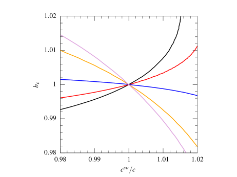
Figure 3: Left panel: Ratio of median concentrations of constrained and unconstrained halos, $c^{\rm co}/c$, as a function of the halo overdcensity $\delta_{\rm h}$ scaled to the rms matter density contrast $\sigma_{0}$ for halos of several virial masses in the Planck14 cosmology. Right panel: Bias parameter $b_{\rm c}$ (i.e. $b_{v}$ for $v=c$) commonly used in numerical studies of the secondary bias as a function of $c^{\rm co}/c$. (A color version is available in the online journal.)

As shown in Section 3.2, the density contrast of the equivalent unconstrained peaks leading to the average density profile of constrained halos with $M_{0}$ at $t_{0}$ (or redshift $z_{0}$) is $\delta_{\rm e0}=\delta_{0}-q\delta_{\rm m}$, which is smaller than $\delta_{0}$. Consequently, the collapse time of the equivalent unconstrained halos, $t_{\rm e}=t(\delta_{0}-q\delta_{\rm m})$, is larger than $t_{0}$ (and the corresponding redshift $z_{\rm e}\equiv z(t_{\rm e})$ smaller than $z_{0}$). As mentioned, CUSP allows one to compute the density profile of unconstrained halos and, from it, their median concentration. Specifically, unconstrained halos with mass $M_{0}$ at $t_{0}$ (or $z_{0}$) have the characteristic mass $M_{\rm c}$ (eq. [18]), total radius $r_{0}$ (eq. [19]), and median concentration $c$ (Salvador-Solé et al., 2023)

$$c=\frac{r_{0}}{r_{\rm c\ast}}\left(\frac{M_{\rm c}}{M_{\rm c\ast}}\right)^{-\tau(M_{\rm c},t_{0})},$$ (20)

where

$$\tau(M_{\rm c},t_{0})=\tau_{\rm c\ast}\left[1+t_{1}\left(\frac{M_{\rm c}}{M_{\rm c\ast}}\right)^{t_{2}}(1+z_{0})^{t_{3}}\right],\\$$ (21)

with coefficients $\tau_{\rm c\ast}$, $r_{\rm c\ast}$, $M_{\rm c\ast}$, $t_{1}$, $t_{2}$, and $t_{3}$ given in Table 3.

This relation also holds, of course, for the equivalent unconstrained halos collapsing at $t_{\rm e}$ (redshift $z_{\rm e}$). Given that the equivalent unconstrained halos grow inside-out, their average density profile at $t_{0}$ is also of the NFW form with the same core radius and a smaller concentration $c^{\rm co}$ because the total radius is smaller, $r^{\rm co}_{0}<r_{\rm e}$. Thus, using the redshift dependence of the median concentration of unconstrained halos, $c\propto(1+z)^{-1}$ (Salvador-Solé et al., 2023), we have

$$c^{\rm co}=c_{\rm e}\,\frac{1+z_{\rm e}}{1+z_{0}}.$$ (22)

As mentioned, the higher the background density $\delta_{\rm m}(t_{0})$, the lower $z_{\rm e}$, so equation (22) states that the smaller $c^{\rm co}$ compared to $c_{\rm e}$. But $c^{\rm co}$ compared to $c$ also depends on $M_{0}$ because $c_{\rm e}$ does. Specifically, taking into account that the unconstrained halos with concentrations $c_{\rm e}$ and $c$ satisfy equations (20)-(21) for the total radii $r_{\rm e}$ and $r_{0}$, characteristic masses $M_{\rm ce}$ and $M_{\rm c}$, and times $t_{\rm e}$ and $t_{0}$, respectively, equation (22) leads to

$$\frac{c^{\rm co}}{c}\!=\frac{(M_{\rm c}/M_{\rm c\ast})^{\tau(M_{\rm c},t_{0})}}{(M_{\rm ce}/M_{\rm c\ast})^{\tau(M_{\rm ce},t_{\rm e})}}\left[\frac{\Delta_{\rm vir}(t_{0})}{\Delta_{\rm vir}(t_{\rm e})}\right]^{1/3}.$$ (23)

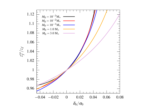
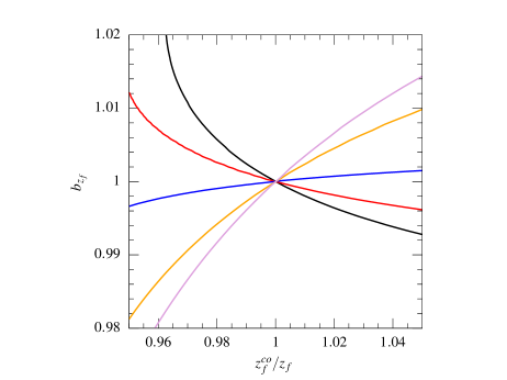
Figure 4: Same as Figure 3 but for the halo formation time. The limits in the abscissa of the left panel correspond to those of in the left panel of that Figure. (A color version is available in the online journal.)

The predicted dependence of the typical concentration $c^{\rm co}$ of halos with $M_{0}$ at $t_{0}$ lying in an overdensity region $\delta_{\rm h}$ of halos with $M_{0}$ is shown in the left panel of Figure 3, while in the right panel we show the dependence of $b_{\rm c}$ (i.e. $b_{v}$ for $v=c$) for halos with $M_{0}$ and $c^{\rm co}$ at $t_{0}$. In the latter plot we see that, as found in simulations, for low-mass halos the higher the concentration, the higher $b_{\rm c}\equiv b^{\rm co}/b$, while the opposite is true for high-mass halos (compare this panel with Fig. 4 of Wechsler et al. 2006). However, as seen in the left panel, the typical value of $c^{\rm co}/c$ is monotonically decreasing with increasing $\delta_{\rm h}$ regardless of the halo mass. In other words, as mentioned at the beginning of this Section, the reversal of the $b_{\rm c}$ vs. $c^{\rm co}/c$ relation from low to high masses has no physical relevance.

4.2 Formation Time

The formation time $t_{\rm f}$ (or formation redshift $z_{\rm f}$) of a halo with $M_{0}$ at $t_{0}$ is defined as the time (redshift) at which the halo reached half its current mass. Since the higher the concentration of a halo, the larger its mass fraction at small radii, the earlier they have also formed.

Specifically, the half-mass radius $r_{\rm h}$ is related to the formation time, $t_{\rm f}$ of unconstrained halos with $M_{0}$ at $t_{0}$ through (eq. [19])

$$r_{\rm h}=\left[\frac{3M_{0}/2}{4\pi\Delta_{\rm vir}(t_{\rm f})\bar{\rho}(t_{\rm f})}\right]^{1/3}.$$ (24)

On the other hand, in NFW halos with mass $M_{0}$, radius $r_{0}$, and concentration $c$, the mass inside the radius $r$ satisfies the relation

$$M(r)=M_{0}\,\frac{f(c\,r/r_{0})}{f(c)}\,,$$ (25)

implying that the radius $r_{\rm h}$ encompassing half their total mass is the solution of the implicit equation

$$\frac{f(c\,r_{\rm h}/r_{0})}{f(c)}=0.5.$$ (26)

Therefore, equation (26) with $r_{\rm h}$ given by equation (24) is an implicit equation for the formation time $t_{\rm f}$ of halos with $M_{0}$ at $t_{0}$.

The previous relations also hold, of course, for the equivalent unconstrained halos (of the NFW form) with $M_{0}$ at $t_{0}$ by simply replacing $c$ by $c^{\rm co}$. Consequently, taking into account that $\Delta_{\rm vir}$ and $f$ are very smooth functions of their respective arguments, both implicit equations lead, after some algebra, to the following relation between the typical formation redshift $z^{\rm co}_{\rm f}$ of constrained and unconstrained halos with $M_{0}$ at $t_{0}$

$$\frac{z^{\rm co}_{\rm f}}{z_{\rm f}}\approx 1+\left(\,\frac{c}{c^{\rm co}}-1\right)\frac{1+z_{\rm f}}{z_{\rm f}}.$$ (27)

Since the more strongly clustered halos, the less concentrated, equation (27) shows that the larger their formation redshift. As can be seen in Figure 2, the dependence of the formation redshift with $\delta_{\rm m}(t_{0})$ is substantially steeper than that of the concentration, and shows the opposite trend. However, the plots in each panel of Figure 4 are identical (very similar in other cases below) to those of Figure 3 except for the opposite trend of the curves. In particular, in the right panel of Figure 4 we see the same reversal of the trend in the $b_{z_{\rm f}}$ vs. $z_{\rm f}^{\rm co}/z_{\rm f}$ relation from low to high masses. We remark that constrained halos with very low masses (say, with $M_{0}<10^{-1}M_{\star}$) will form at such high redshifts that their mass at formation will often fall below the halo mass limit of simulations, so they will not be included in numerical studies of this bias. As a consequence, the reversal of the trend should be more difficult to detect for the formation redshift than for the concentration, which explains the doubts about that particular feature regarding the formation time found in the literature (e.g. Jing, Suto, & Mo 2007 and Gao & White 2007).

4.3 Peak Velocity

The peak velocity $v_{\rm p}$ of a halo is the maximum value reached by its circular velocity profile $V(r)$ defined as

$$V(r)=\left[\frac{GM(r)}{r}\right]^{1/2},$$ (28)

where $M(r)$ is the mass inside $r$ and $G$ is the gravitational constant. Obviously, the more concentrated a halo of a given total mass, the steeper the profile $M(r)$, so the higher also peaks the circular velocity. Let us put this in a more quantitative way.

The radius $r_{\rm max}$ marking the peak velocity satisfies

$$\frac{V(r_{\rm max})}{2r_{\rm max}}\left[\frac{{\rm d}\ln M}{{\rm d}\ln r}\bigg{|}_{r_{\rm max}}-1\right]=0,$$ (29)

implying $4\pi r_{\rm max}^{3}\rho(r_{\rm max})=M(r_{\rm max})$, which, in NFW halos with $M_{0}$ and $r_{0}$ at $t_{0}$, leads to $r_{0}/(c\,r_{\rm max})=f^{-1/2}(c\,r_{\rm max}/r_{0})-1$. Plugging such an expression of $r_{\rm max}$ into equation (28) and using the NFW expression for $M(r_{\rm max})/r_{\rm max}$, we obtain

$$V_{\rm max}=\left[\frac{GM_{0}}{r_{0}}\frac{h(c\,r_{\rm max}/r_{0})}{h(c)}\right]^{1/2},$$ (30)

where $h(x)$ stands for $f(x)/x$.

Replacing $c$ by $c^{\rm co}$, we obtain the homologous expression for halos of the same mass $M_{0}$ at the same time $t_{0}$ but lying in a background. And, using both relations, we arrive at the following ratio between the peak velocity $V^{\rm co}_{\rm max}$ in constrained halos and the value $v_{\rm p}$ in unconstrained ones,

$$\frac{V^{\rm co}_{\rm max}}{V_{\rm max}}=\left[\frac{h(c)}{h(c^{\rm co})}\right]^{1/2},$$ (31)

where we have used that $h[(c\,r_{\rm max})^{\rm co}/r_{0}]$ equals $h[(c\,r_{\rm max})/r_{0}]$ as $c\,r_{\rm max}/r_{0}$ and $(c\,r_{\rm max})^{\rm co}/r_{0}$ are solutions of the same implicit equation mentioned above.

In Figure 2 we see that the $V^{\rm co}_{\rm max}/V_{\rm max}$ decreases with increasing $\delta_{\rm m}(t_{0})$ like $c^{\rm co}/c$ though substantially less steeply. In this sense, even though the peak velocity is often used to evidence the concentration bias because $V\max$ is simpler to measure than $c$ (e.g. Gao & White 2007; Angulo, Baugh, & Lacey 2008), one must bear in mind that the former has a much less marked bias than the latter. What is instead a very good indicator (though with the opposite trend) of the concentration bias is the bias in the peak velocity radius since the latter equality mentioned above implies $r_{\rm max}^{\rm co}/r_{\rm max}=c/c^{\rm co}$.

4.4 Subhalo Abundance

The results of Section 3 were obtained assuming purely accreting halos. This was justified because the properties of halos with $M_{0}$ at $t_{0}$ do not depend on their merger history. But, as mentioned, there is one exception: the properties related to substructure. In particular, the subhalo abundance down to a fixed scaled subhalo mass, $M_{\rm s}/M_{0}$, $N_{\rm s}$, depends on the time $t_{\rm m}$ of the last major merger of the halo (Salvador-Solé, Manrique & Botella, 2022a, b; Salvador-Solé et al., 2022). Strictly speaking, $t_{\rm m}$ is not the same as the halo formation time $t_{\rm f}$. But, since halos essentially double their mass in major mergers (e.g. Raig, González-Casado & Salvador-Solé 2001), we can take the latter as a good proxy of the former.

The dependence on $t_{\rm f}$ of $N_{\rm s}$ is quite convoluted: apart from depending on the accretion rate of the host halo (Salvador-Solé, Manrique & Botella, 2022a), it depends on its concentration determining the strength at which accreted subhalos are tidally stripped by the halo potential well (Salvador-Solé, Manrique & Botella, 2022b) and the halo merger history Salvador-Solé et al. (2022). However, as found in the latter work, $\log N_{\rm s}$ in the 20% of unconstrained halos with $M_{0}$ at $t_{0}$ having suffered the last merger before $0.28t_{0}$ is $\approx 3/2$ times that of the 20% of objects having suffered it after $0.76t_{0}$. Thus, adopting the approximation that the merger of the two kinds of halos took place just the time delimiting their respective intervals, we are led to

$$\log(N_{\rm s}/N_{\rm s0})\sim-A\log(t_{\rm f}/t_{0}),$$ (32)

where $N_{\rm s}$ and $N_{\rm s0}$ are the subhalo abundances of unconstrained halos with $M_{0}$ at $t_{0}$ formed at $t_{\rm f}$ and at any time, respectively, and factor $A$ satisfies the equation $\log(3/2)=-A(\log 0.28-\log 0.76)$ is $A\sim 0.41$.

Relation (32) holds for unconstrained halos of any mass at any time, so it hold for unconstrained halos with $M_{0}$ at $t_{0}$ and with $M_{0}$ at $t_{\rm e0}=t(\delta_{0}-\delta_{\rm m})$, and, dividing both relations, we are led to

$$\frac{N^{\rm co}_{\rm s}}{N_{\rm s}}\approx\left(\frac{t_{\rm f}^{\rm co}t_{0}}{t_{\rm f}t_{\rm e0}}\right)^{-0.41}\frac{N_{\rm se}}{N_{\rm s0}},$$ (33)

where $N_{\rm s}$ and $N_{\rm se}$ are the subhalo abundances (down to the same scaled subhalo mass) of unconstrained halos with $M_{0}$ at the times $t_{0}$ and $t_{\rm e}$, respectively. As shown in Salvador-Solé et al. (2022), the average subhalo abundance scales with the mass $M_{0}$ of halos (with their own typical concentration) as $N_{\rm s}\propto(M_{0}/10^{12}$M_⊙$)^{0.08}$, with the same proportionality factor at any time $t_{0}$. Since both kinds of unconstrained halos have identical mass $M_{0}$, the last factor on the right of equation (33) cancels and we arrive at

$$\frac{N^{\rm co}_{\rm s}}{N_{\rm s}}\approx\left(\frac{t_{\rm f}t_{\rm e0}}{t_{\rm f}^{\rm co}t_{0}}\right)^{0.41}.$$ (34)

Given that the higher $\delta_{\rm m}(t_{0})$, the earlier halos form and the later they collapse, equation (34) tells that the larger their amount of subhalos, in agreement with the results of simulations. Both characteristic times are functions of the concentration (Secs. 4.1 and 4.2), so the subhalo abundance in halos with the average density profile coincides with its median value, like in all preceding properties. Figure 4 shows that the bias in the subhalo abundance is very similar to that in the formation redshift.

4.5 Kinematics

The velocity dispersion $\sigma(r)$ and anisotropy $\beta(r)$ profiles of haloes with $M_{0}$ at $t_{0}$ are related to the curvature, ellipticity, and prolateness of the corresponding peaks in a convoluted non-analytic way that involves, in addition, their triaxial shape Salvador-Solé et al. (2012b). However, taking into account the gravitational origin of the velocity anisotropy and energy conservation, in the final objects, they satisfy very simple theoretical relations with the density profile alone in agreement with the results of simulations: one regarding the pseudo-phase space density profile $\rho(r)/\sigma^{3}(r)$ (Bertschinger, 1985; Tylor & Navarro, 2001)

$$\sigma(r)\propto\rho^{1/3}(r)r^{1.875/3},$$ (35)

with a universal proportionality constant, and the other regarding the velocity anisotropy profile $\beta(r)$ (Hansen & Stadel, 2006)

$$\beta(r)\approx-0.2\left(\frac{{\rm d}\ln\rho}{{\rm d}\ln r}+0.8\right).$$ (36)

In other words, both kinematic properties turn out to be fully determined by the density profile itself. The ultimate reason for this is clear: as mentioned in Section 2, the typical ellipticity and prolateness of peaks at a given scale are functions of their density contrast and average curvature only.

Thus, since the average density profiles of constrained and unconstrained halos are slightly different, the same is true for their average velocity dispersion and anisotropy profiles. Specifically, the higher the background density, the more concentrated the halo, and hence, the steeper its density profile. Consequently, the steeper also the velocity dispersion and anisotropy profiles.

More concretely, dividing the relations (35) holding for constrained and unconstrained halos, we are led to

$$\frac{\sigma^{\rm co}(r)}{\sigma(r)}=\left[\frac{\rho^{\rm co}(r)}{\rho(r)}\right]^{1/3}.$$ (37)

In particular, at the virial radius where $\rho(r_{0})=M_{0}c^{2}/(4\pi r_{0}^{3})/[f(c)(1+c)^{2}]$ we have

$$\frac{\sigma^{\rm co}(r_{0})}{\sigma(r_{0})}=\left[\left(\frac{c^{\rm co}}{c}\frac{1+c}{1+c^{\rm co}}\right)^{2}\frac{f(c)}{f(c^{\rm co})}\right]^{1/3}.$$ (38)

Since the higher $\delta_{\rm m}(t_{0})$, the higher $c^{\rm co}>c$, equation (35) tells that the higher also $\sigma^{\rm co}(r_{0})$, in agreement with simulations (see Fig. 2).

On the other hand, dividing the relations (36) at the virial radius $r_{0}$ for the unconstrained and constrained halos, with concentrations $c$ and $c^{\rm co}$, respectively, where the logarithmic slope of the density profile of NFW halos with $M_{0}$ and $r_{0}$ satisfies

$$\frac{{\rm d}\ln\rho}{{\rm d}\ln r}=-\left[1+\frac{2}{1+r_{0}/(rc)}\right],$$ (39)

we arrive at

$$\frac{\beta^{\rm co}(r_{0})}{\beta(r_{0})}\approx\frac{0.1+1/[1+(c^{\rm co})^{-1}]}{0.1+1/(1+c^{-1})}.$$ (40)

Since the higher $\delta_{\rm m}(t_{0})$, the higher $c^{\rm co}$, equation (40) tells that the smaller $\beta^{\rm co}(r_{0})$ (see Fig. 2).

As can be seen in Figure 2, the bias in the velocity dispersion and anisotropy is the less marked among all the properties analyzed. Nevertheless, for the above mentioned reason, the corresponding $b_{v}$ vs. $v^{\rm co}/v$ plots are very similar to those for the concentration and the formation redshift (Figs. 3 and 4).

4.6 Triaxial Shape

As mentioned, the triaxial shape of halos, characterized by their ellipticity ($e\geq 0$) and prolateness ($|p|\leq e$, with $p$ positive for oblate objects and negative for prolate ones), is related to that of the corresponding peaks through the kinematics of the final objects in a convoluted non-analytic way. However, Salvador-Solé et al. (2012b) showed that, globally, the shape of the isodensity contours in halos and protohalos vary with radius in a similar way. Moreover, since the deeper one goes within both objects, the less marked is the influence of the kinematics in the halo shape, the closer their triaxial shape. On the contrary, halos become increasingly more spherical than their seeds outwards. Thus, we will concentrate on the halo shape at small radii for which simple analytic relations can be derived.

The probability of a given ellipticity and prolateness of peaks is independent of their height $\nu$ and decreases with increasing curvature (BBKS). In particular, the typical asphericity of peaks with $\delta_{0}$ at $R_{0}$ measured through the ellipticity $e$ diminishes with the average curvature $\langle x\rangle$.

$$e\approx\frac{1}{\sqrt{5}}\left[\langle x\rangle^{2}(R_{0},\delta_{0})+6/5\right]^{-1/2}.$$ (41)

Since constrained peaks with $\delta_{0}$ at $R_{0}$ behave as unconstrained ones with $\delta_{\rm e0}=\delta_{0}-q\delta_{\rm m}$ at$R_{0}$, their median ellipticity takes the form (41) with the average curvature evaluated at $\delta_{\rm e0}$. Consequently, the ratio of median ellipticities at small radii (e.g. $r\sim r_{\rm c}$) of constrained and unconstrained halos with large $M_{0}$ at $t_{0}$, close to those of their corresponding peaks, is

$$\frac{e^{\rm co}}{e}\approx\left[\frac{\langle x\rangle^{2}(R_{0},\delta_{0})+6/5}{\langle x\rangle^{2}(R_{0},\delta_{\rm e0})+6/5}\right]^{1/2}.$$ (42)

Since $\langle x\rangle(R,\delta)$ increases with increasing $\delta$ at fixed $R$, equation (42) implies that the larger $\delta_{\rm m}(t_{0})$, the larger the typical ellipticity $e^{\rm co}$. And, in lower mass halos, the dependence of $e^{\rm co}/e$ on $c^{\rm co}/c$ is less simple, but the trend is similar. As shown in Figure 2, the ellipticity bias (at small radii and for large mass halos) is quite weak, which agrees with the results of observations (Chen et al., 2020). In fact, the trend of the shape bias is reversed at high masses, the frontier between both regimes being at the same mass as marking the frontier of the two regimes in the concentration bias as found in simulations by Faltenbacher & White (2010).

The same derivation applied to the halo prolateness $p$ leads to a ratio of prolatenesses $p^{\rm co}/p$ in constrained and unconstrained halos of the same form as $e^{\rm co}/e$, but with the right hand member of equation (42) to the fourth power.

4.7 Spin

The spin parameter $\lambda$ used in most studies of the secondary bias (e.g. Gao & White 2007) is defined as (Bullock et al., 2001)

$$\lambda=\frac{J}{\sqrt{2}M_{0}r_{0}V_{0}},$$ (43)

where $J$ is the modulus (vector norm) of the total angular momentum (AM) ${\bf J}$ relative to center of mass (c.o.m.) of the halo with $M_{0}$, and $V_{0}$ is its circular velocity at the radius $r_{0}$. According to the Tidal Torque Theory, in linear and moderately non-linear regime ${\bf J}$ is kept with the same direction and $J$ increases with time $t$ as $J(t)=a^{2}(t)\dot{D(t)}\,J^{\rm L}$, where

$$J_{i}^{\rm L}=\epsilon_{ijk}{\bf T}_{jl}{\bf I}_{lk}$$ (44)

is the $i$th component of the constant Lagrangian protohalo AM, ${\bf T}$ is the Hessian of the potential at the c.o.m. of the protohalo at $t_{\rm i}$ and I is its inertia tensor (White, 1984). Therefore, the ratio of the median AM of constrained and unconstrained halos with $M_{0}$ collapsed at the same time $t_{0}$, $J^{\rm co}/J$, is simply equal to the ratio of their median Lagrangian AM modulus, $(J^{\rm L})^{\rm co}/J^{\rm L}$.

Using CUSP Salvador-Solé & Manrique (2024b) have derived the median Lagrangian AM of unconstrained halos with virial mass $M_{0}$ at $t_{0}$ in the peak model, the result being

$$J^{\rm L}(M_{0},t_{0})\approx\frac{3.2\!\times\!10^{-2}}{\widetilde{m}+3}G\bar{\rho}^{1/3}_{0}s^{\widetilde{m}}\widetilde{M}_{0}^{5/3}\frac{\delta_{0}}{D(t_{\rm i})},$$ (45)

where $\bar{\rho}_{0}$ is the present mean cosmic density, $\widetilde{m}=-13[(n+3)/2]/3\approx-2.71$ (for the CDM spectral index $n\approx-1.75$ corresponding to galactic haloes),

$$s^{-3}=\!\frac{2}{3\pi}\!\left(\!\frac{n+5}{6}\!\right)^{3/2}G_{0}(\gamma,\gamma\nu)\,{\rm e}^{-\frac{\nu^{2}}{2}},$$ (46)

and

$$\widetilde{M}_{0}=\frac{(\gamma\nu)^{2}}{\langle x\rangle^{2}(R_{0},\delta_{0})+6/5}\,M_{0}.$$ (47)

Note that $J^{\rm L}(M_{0},t_{0})$ is independent of the (arbitrary) initial time $t_{\rm i}$ because $\delta_{0}/D(t_{\rm i})$ is a function of $t_{0}$ alone (see eq. [1]). Therefore, taking into account that $V_{0}$ is the same in constrained and unconstrained halos with $M_{0}$ and $r_{0}$ (eq. [28]), we are led to

$$\frac{\lambda^{\rm co}}{\lambda}\!=\!\frac{J^{\rm co}}{J}\!\approx\!\left[\frac{\langle x\rangle^{2}(R_{0},\delta_{0})+6/5}{\langle x\rangle^{2}(R_{0},\delta_{\rm e0})+6/5}\right]^{5/3}.$$ (48)

Given that the higher the background $\delta_{\rm m}$, the smaller $\langle x\rangle(R_{0},\delta_{\rm e0})$, we have that the larger the spin as found in simulations (Gao & White, 2007). In Figure 2 we see that the spin is among the properties (together with concentration, formation redshift, and subhalo abundance) that show the most marked bias, in agreement with the results of simulations (Mao, Zentner & Wechsler, 2018). In addition, the common origin (related to the average curvature of protohalos) of the shape and spin biases is consistent with their observed correlation Sato-Polito et al. (2019).

Note that, since the time $t_{0}$ during which the tidal torque is acting on constrained and unconstrained protohalos is the same and cancels in the ratio $\lambda^{\rm co}/\lambda$, the spin bias coincides with the bias in the tidal torque suffered by halos also studied by means of simulations (Hahn et al., 2009; Ramakrishnan & Paranjape, 2020).

5 SUMMARY AND CONCLUSIONS

Cosmological simulations show that halos with the same mass but different internal properties or formation times are differently clustered, which is known as the secondary (or assembly) halo bias.

Using the CUSP formalism linking halos with mass $M_{0}$ at the cosmic time $t_{0}$ with peaks with density contrast $\delta_{0}$ at scale $R_{0}$ in the Gaussian-smoothed random Gaussian density field at an initial time $t_{\rm i}$, we have examined the appealing idea, suggested by Dalal et al. (2008), that the secondary bias arises from the fact that peaks with $\delta_{0}$ at $R_{0}$ lying in different backgrounds have different typical curvatures.

We have shown that, except for the triaxial shape and spin of halos, which directly arise form the curvature of their associated peaks, all the remaining properties, namely the concentration, formation time, velocity peak, subhalo abundance, and kinematics, arise from the curvature of peaks associated with the continuous sequence of progenitors along their accretion history. Indeed, as shown in Salvador-Solé & Manrique (2021), the average density profile of halos with $M_{0}$ at $t_{0}$ arises from the mean $\delta(R)$ trajectory followed by peaks in the filtering process tracing halo accretion, which is determined in turn by the average curvature of peaks at each point of the trajectory setting the instantaneous accretion rate of the corresponding progenitor. Since the average curvature of peaks depends on their background density, the average density profile of halos and their shape and spin depend on the corresponding halo background. This causes not only the concentration of halos with $M_{0}$ at $t_{0}$ but also any other property related to their density profile and the shape and spin as well to depend on the halo background, or equivalently (due to the primary halo bias), on the halo clustering level.

Interestingly, the average curvature of peaks lying in a background is essentially the same as for unconstrained peaks of the same scale but a slightly different density contrast. This has allowed us to derive simple analytic expressions for the bias of all halo properties. The predicted typical (median) values of all these properties in halos with a specific clustering level, or equivalently, the clustering level (measured though the $b_{v}$ parameter) of halos with specific values of the properties agree with the trends found in simulations.

One unexpected result we have found is that the only difference between distinct properties is the relation between their values and the background density, that is, the median value vs. halo overdensity and $b_{v}$ vs. specific value relations are identical for all properties. In particular, the reversal of the latter relation when going from low to high halo masses is a general feature arising from the dependence of the average peak curvature on density contrast and scale; it does not reflect the change in the clustering of any halo property with mass. In fact, the higher the halo overdensity, the higher or lower is always the typical values of any property regardless of halo mass.

Thus, the main conclusions of this work is that the secondary halo bias, like the primary one, is innate and is well reproduced in the peak model of structure formation.

References

- Angulo, Baugh, & Lacey (2008) Angulo R. E., Baugh C. M., Lacey C. G., 2008, MNRAS, 387, 921
- Bahcall & Soneira (1983) Bahcall N. A., Soneira R. M., 1983, ApJ, 270, 20
- Barber et al. (2012) Barber, J.A., Zhao, H., Wu, X., & Hansen, S. H. 2012, MNRAS, 424, 1737
- Bardeen et al. (1986) Bardeen J. M., Bond J. R., Kaiser N., Szalay A. S., 1986, ApJ, 304, 15 (BBKS)
- Bertschinger (1985) Bertschinger, E. 1985, ApJS, 58, 39
- Bond et al. (1991) Bond, J.R., Cole, S., Efstathiou, G., & Kaiser, N. 1991, ApJ, 379, 440
- Bryan & Norman (1998) Bryan G.L. & Norman M. L., 1998, ApJ, 495, 80
- Bullock et al. (2001) Bullock J. S., Dekel A., Kolatt T. S., Kravtsov A. V., Klypin A. A., Porciani C., Primack J. R., 2001, ApJ, 555, 240
- Capelato et al. (1980) Capelato H. V., Gerbal D., Salvador-Sole E., Mathez G., Mazure A., Sol H., 1980, ApJ, 241, 521
- Chen et al. (2020) Chen Y., Mo H. J., Li C., Wang H., Yang X., Zhang Y., Wang K., 2020, ApJ, 899, 81
- Dalal et al. (2008) Dalal N., White M., Bond J. R., Shirokov A., 2008, ApJ, 687, 12
- Desjacques (2008) Desjacques V., 2008, MNRAS, 388, 638
- Dressler (1980) Dressler A., 1980, ApJ, 236, 351
- Dressler et al. (1997) Dressler A., Oemler A., Couch W. J., Smail I., Ellis R. S., Barger A., Butcher H., et al., 1997, ApJ, 490, 577 (D+97)
- Einasto (1965) Einasto J. 1965, Trudy Inst. Astrofiz. Alma-Ata, 5, 87
- Ellis et al. (1997) Ellis R. S., Smail I., Dressler A., Couch W. J., Oemler A., Butcher H., Sharples R. M., 1997, ApJ, 483, 582
- Faber & Gallagher (1979) Faber S. M., Gallagher J. S., 1979, ARA&A, 17, 135
- Faltenbacher & White (2010) Faltenbacher, A. & White, S. D. M. 2010, ApJ, 708, 469
- Fakhouri & Ma (2009) Fakhouri O., Ma C.-P., 2009, MNRAS, 394, 1825
- Fakhouri & Ma (2010) Fakhouri, O., & Ma, C.-P. 2010, MNRAS, 401, 2245
- Gao, Springel, & White (2005) Gao L., Springel V., White S. D. M., 2005, MNRAS, 363, L66
- Gao & White (2007) Gao L., White S. D. M., 2007, MNRAS, 377, L5
- Gottlöber, Klypin, & Kravtsov (2001) Gottlöber S., Klypin A., Kravtsov A. V., 2001, ApJ, 546, 223
- Gottlöber et al. (2002) Gottlöber S., Kerscher M., Kravtsov A. V., Faltenbacher A., Klypin A., Müller V., 2002, A&A, 387, 778
- Hahn et al. (2009) Hahn O., Porciani C., Dekel A., Carollo C. M., 2009, MNRAS, 398, 1742
- Hansen et al. (2006) Hansen, S. H., Moore, B., Zemp, M., et al. 2006, J. Cosmology Astropart. Phys, 1
- Hansen & Stadel (2006) Hansen S. H., Stadel J., 2006, JCAP, 2006, 014
- Harker et al. (2006) Harker G., Cole S., Helly J., Frenk C., Jenkins A., 2006, MNRAS, 367, 1039
- Hauser & Peebles (1973) Hauser M. G., Peebles P. J. E., 1973, ApJ, 185, 757
- Hellwing et al. (2021) Hellwing W. A., Cautun M., van de Weygaert R., Jones B. T., 2021, PhRvD, 103, 063517
- Henry (2000) Henry, J. P. 2000, ApJ, 534, 565
- Hester & Tasitsiomi (2010) Hester J. A., Tasitsiomi A., 2010, ApJ, 715, 342
- Huss et al. (1999) Huss, A., Jain, B.,& Steinmetz, M. 1999, ApJ, 517, 64
- Jing, Suto, & Mo (2007) Jing Y. P., Suto Y., Mo H. J., 2007, ApJ, 657, 664
- Juan et al. (2014a) Juan E., Salvador-Solé E., Domènec G., Manrique A., 2014, MNRAS, 439, 719
- Kaiser (1984) Kaiser N., 1984, ApJL, 284, L9
- Komatsu et al. (2011) Komatsu E., Smith K. M., Dunkley J., Bennett C. L., Gold B., Hinshaw G., Jarosik N., et al., 2011, ApJS, 192, 18
- Lazeyras et al. (2023) Lazeyras, T., Barreira, A., Schmidt, F., et al. 2023, J. Cosmology Astropart. Phys, 2023, 023
- Lee et al. (2017) Lee C. T., Primack J. R., Behroozi P., Rodríguez-Puebla A., Hellinger D., Dekel A., 2017, MNRAS, 466, 3834
- Macciò et al. (2007) Macciò, A. V., Dutton, A. A., van den Bosch, F. C., et al. 2007, MNRAS, 378, 55
- Mao, Zentner & Wechsler (2018) Mao Y.-Y., Zentner A. R., Wechsler R. H., 2018, MNRAS, 474, 5143
- Manrique & Salvador-Solé (1995) Manrique A. & Salvador-Solé E., 1995, ApJ, 453, 6
- Manrique & Salvador-Solé (1996) Manrique A. & Salvador-Solé E., 1996, ApJ, 467, 504
- Manrique et al. (1998) Manrique A., Raig A., Solanes J. M., González-Casado G., Stein, P., Salvador-Solé E., 1998, ApJ, 499, 548
- Mo et al. (2005) Mo H. J., Yang X., van den Bosch F. C., Katz N., 2005, MNRAS, 363, 1155
- Montero-Dorta et al. (2020) Montero-Dorta A. D., Artale M. C., Abramo L. R., Tucci B., Padilla N., Sato-Polito G., Lacerna I., et al., 2020, MNRAS, 496, 1182
- Mo & White (1996) Mo H. J., White S. D. M., 1996, MNRAS, 282, 347
- Moore et al. (1999) Moore B., Quinn T., Governato F., Stadel J., Lake G., 1999, MNRAS, 310, 114
- Navarro, Frenk & White (1995) Navarro J. F., Frenk C. S, White S. D. M., 1995, ApJ, 275, 720
- Peacock & Smith (2000) Peacock J. A., Smith R. E., 2000, MNRAS, 318, 1144
- Peebles (1969) Peebles P. J. E., 1969, ApJ, 155, 393. doi:10.1086/149876
- Planck Collaboration et al. (2014) Planck Collaboration, Ade, P. A. R., Aghanim, N., et al. 2014, A&A, 571, AA16
- Poggianti et al. (1999) Poggianti B. M., Smail I., Dressler A., Couch W. J., Barger A. J., Butcher H., Ellis R. S., et al., 1999, ApJ, 518, 576
- Press & Schechter (1974) Press, W. H.,& Schechter, P. 1974, ApJ, 187, 425
- Raig, González-Casado & Salvador-Solé (2001) Raig A., González-Casado G., Salvador-Solé E., 2001, MNRAS, 327, 939
- Ramakrishnan & Paranjape (2020) Ramakrishnan S., Paranjape A., 2020, MNRAS, 499, 4418
- Salvador-Solé, Manrique, & Solanes (2005) Salvador-Solé E., Manrique A., Solanes J. M., 2005, MNRAS, 358, 901
- Salvador-Solé et al. (2012a) Salvador-Solé, E., Viñas, J., Manrique, A., & Serra, S. 2012a, MNRAS, 423, 2190
- Salvador-Solé et al. (2012b) Salvador-Solé, E., Serra, S., Manrique, A., & González-Casado, G. 2012b, MNRAS, 424, 3129
- Salvador-Solé & Manrique (2021) Salvador-Solé E., Manrique A., 2021, ApJ, 914,141
- Salvador-Solé, Manrique & Botella (2022a) Salvador-Solé E., Manrique A., Botella I., 2022, MNRAS, 509, 5305
- Salvador-Solé, Manrique & Botella (2022b) Salvador-Solé E., Manrique A., Botella I., 2022, MNRAS, 509, 5316
- Salvador-Solé et al. (2022) Salvador-Solé E., Manrique A., Canales D., Botella I., 2022, MNRAS, 511, 641
- Salvador-Solé et al. (2023) Salvador-Solé E., Manrique A., Canales D., Botella I., 2023, MNRAS, 521, 1988
- Salvador-Solé & Manrique (2024a) Salvador-Solé E., Manrique A., 2024, accepted for publication in ApJ(Paper I).
- Salvador-Solé & Manrique (2024b) Salvador-Solé E., Manrique A., 2024, submitted to MNRAS.
- Sandvik et al. (2007) Sandvik H. B., Möller O., Lee J., White S. D. M., 2007, MNRAS, 377, 234
- Sanromà & Salvador-Solé (1990) Sanroma M., Salvador-Sole E., 1990, ApJ, 360, 16
- Sato-Polito et al. (2019) Sato-Polito G., Montero-Dorta A. D., Abramo L. R., Prada F., Klypin A., 2019, MNRAS, 487, 1570
- Seljak (2000) Seljak U., 2000, MNRAS, 318, 203
- Sheth & Tormen (2004) Sheth R. K., Tormen G., 2004, MNRAS, 350, 1385
- Smith et al. (2005) Smith G. P., Treu T., Ellis R. S., Moran S. M., Dressler A., 2005, ApJ, 620
- Tylor & Navarro (2001) Taylor, J. E., & Navarro, J. F. 2001, ApJ, 563, 483
- Wang et al. (2020) Wang K., Mao Y.-Y., Zentner A. R., Lange J. U., van den Bosch F. C., Wechsler R. H., 2020, MNRAS, 498, 4450
- Wang & White (2009) Wang, J., & White, S. D. M. 2009, MNRAS, 396, 709
- White (1984) White, S. D. M. 1984, ApJ, 286, 38
- Wechsler et al. (2006) Wechsler R. H., Zentner A. R., Bullock J. S., Kravtsov A. V., Allgood B., 2006, ApJ, 652, 71
- Wetzel et al. (2007) Wetzel A. R., Cohn J. D., White M., Holz D. E., Warren M. S., 2007, ApJ, 656, 139
- Xu & Zheng (2020) Xu X., Zheng Z., 2020, MNRAS, 492, 2739. doi:10.1093/mnras/staa009
- Yu et al. (2017) Yu H. R., Emberson J., Inman D. et al., 2017, Nat Astron 1, 0143
- Zentner (2007) Zentner, A. R. 2007, International Journal of Modern Physics D, 16, 763
- Zentner et al. (2005) Zentner, A. R., Berlind, A. A., Bullock, J. S., et al. 2005, ApJ, 624, 505. doi:10.1086/428898
- Zhu et al. (2006) Zhu G., Zheng Z., Lin W. P., Jing Y. P., Kang X., Gao L., 2006, ApJ, 639, L5