MetaGFN: Exploring Distant Modes with Adapted Metadynamics for Continuous GFlowNets
Abstract
Generative Flow Networks (GFlowNets) are a class of generative models that sample objects in proportion to a specified reward function through a learned policy. They can be trained either on-policy or off-policy, needing a balance between exploration and exploitation for fast convergence to a target distribution. While exploration strategies for discrete GFlowNets have been studied, exploration in the continuous case remains to be investigated, despite the potential for novel exploration algorithms due to the local connectedness of continuous domains. Here, we introduce Adapted Metadynamics, a variant of metadynamics that can be applied to arbitrary black-box reward functions on continuous domains. We use Adapted Metadynamics as an exploration strategy for continuous GFlowNets. We show three continuous domains where the resulting algorithm, MetaGFN, accelerates convergence to the target distribution and discovers more distant reward modes than previous off-policy exploration strategies used for GFlowNets.
1 Introduction
Generative Flow Networks (GFlowNets) are a type of generative model that samples from a discrete space by sequentially constructing objects via actions taken from a learned policy Bengio et al. (2021a). The policy specifies the probability of transitioning from some state to some other state . The policy is parameterised and trained so that, at convergence, the probability of sampling an object is proportional to a specified reward function . GFlowNets offer advantages over more traditional sampling methods, such as Markov chain Monte Carlo (MCMC), by learning an amortised sampler, capable of single-shot generation of samples from the desired distribution. Since GFlowNets learn a parametric policy, they can generalise across states, resulting in higher performance across various tasks Bengio et al. (2021a); Malkin et al. (2022); Zhang et al. (2022); Jain et al. (2022); Deleu et al. (2022); Jain et al. (2023); Hu et al. (2023); Zhang et al. (2023); Shen et al. (2023b) and applications to conditioned molecule generation Shen et al. (2023b), maximum likelihood estimation in discrete latent variable models Hu et al. (2023), structure learning of Bayesian networks Deleu et al. (2022), scheduling computational operations Zhang et al. (2023), and discovering reticular materials for carbon capture Cipcigan et al. (2023).
Although originally conceived for discrete state spaces, GFlowNets have been extended to more general state spaces, such as entirely continuous spaces, or spaces that are hybrid discrete-continuous Lahlou et al. (2023). In the continuous setting, given the current state, the policy specifies a continuous probability distribution over subsequent states, and the probability density over states sampled with the policy is proportional to a reward density function . The continuous domain unlocks more applications for GFlowNets, such as molecular conformation sampling Volokhova et al. (2023) and continuous control problems Luo et al. (2024).
GFlowNets are trained like reinforcement learning agents. Trajectories of states are generated either on-policy or off-policy, with the terminating state providing a reward signal for informing a gradient step on the policy parameters. GFlowNets therefore suffer from the same training pitfalls as reinforcement learning. One such issue is slow temporal credit assignment, which has thus far been addressed by designing more effective loss functions, such as detailed balance Bengio et al. (2021b), trajectory balance Malkin et al. (2022) and sub-trajectory balance Madan et al. (2022).
Besides loss functions, another aspect of GFlowNet training is the exploration strategy for acquiring training samples. Exclusively on-policy learning is generally inadequate as it leads to inefficient exploration of new modes. More successful strategies therefore rely on off-policy exploration. For the discrete setting, numerous exploration strategies have been proposed including -noisy with a uniform random policy, tempering, Generative Augmented Flow Networks (GAFN) Pan et al. (2022), Thompson sampling Rector-Brooks et al. (2023) and Local Search GFlowNets Kim et al. (2024). While these approaches can be generalised to the continuous domain, there is no literature benchmarking their effectiveness in this setting.
Sampling in the continuous setting is a common occurrence in various domains such as molecular modelling Hawkins (2017); Yang et al. (2019) and Bayesian inference Shahriari et al. (2016). The local connectedness of a continuous domain allows for novel exploration strategies that are not directly applicable in the discrete setting. In this work, we create MetaGFN, an exploration algorithm for continuous GFlowNets inspired by metadynamics, an enhanced sampling method widely used for molecular modelling Laio and Parrinello (2002). The main contributions of this work are:
-
•
Presenting MetaGFN, an algorithm created by adapting metadynamics to black box rewards and continuous GFlowNets;
-
•
Proving that the proposed Adapted Metadynamics is consistent and reduces to standard metadynamics in a limit;
-
•
Showing empirically that MetaGFN outperforms existing GFlowNets exploration strategies.
The rest of the paper is as follows. In Section 2 we review the theory of discrete and continuous GFlowNets. We present Adapted Metadynamics and MetaGFN in Section 3. In Section 4, we evaluate MetaGFN against other exploration strategies, showing that MetaGFN outperforms existing exploration strategies in two continuous environments. We finish with limitations and conclusions in Sections 5 and 6. Code for MetaGFN is available at [link in camera-ready].
2 Preliminaries
2.1 Discrete GFlowNets
In a GFlowNet, the network refers to a directed acyclic graph (DAG), denoted as . Nodes represent states , and edges represent actions denoting one-way transitions between states. The DAG has two distinguishable states: a unique source state , that has no incoming edges, and a unique sink state , that has no outgoing edges. The set of states, , that are directly connected to the sink state are known as terminating states. GFlowNets learn forward transition probabilities, known as a forward policy , along the edges of the DAG so that the resulting marginal distribution over the terminal states complete trajectories (the terminal distribution) , denoted as , is proportional to a given reward function . GFlowNets also introduce additional learnable objects, such as a backward policy , which is a distribution over the parents of any state of the DAG, to create losses that train the forward policy. Objective functions for GFlowNets include flow matching (FM), detailed balance (DB), trajectory balance (TB) and subtrajectory balance (STB) Bengio et al. (2021a, b); Malkin et al. (2022); Madan et al. (2022). During training, the parameters of the flow objects are updated with stochastic gradients of the objective function applied to batches of trajectories. These trajectory batches can be obtained either directly from the current forward policy or from an alternative algorithm that encourages exploration. These approaches are known as on-policy and off-policy training respectively.
2.2 Continuous GFlowNets
Continuous GFlowNets extend the generative problem to continuous spaces Lahlou et al. (2023), where the analogous quantity to the DAG is a measurable pointed graph (MPG) Nummelin (1984). MPGs can model continuous spaces (e.g., Euclidean space, spheres, tori), as well as hybrid spaces, with a mix of discrete and continuous components, as often encountered in robotics, finance, and biology Neunert et al. (2020); Swiler et al. (2012); Bortolussi and Policriti (2008).
Definition 2.1 (Measurable pointed graph (MPG)).
Let be a topological space, where is the state space, is the set of open subsets of , and is the Borel -algebra associated with the topology of . Within this space, we identify the source state and sink state , both distinct and isolated from the rest of the space. On this space we define a reference transition kernel and a backward reference transition kernel . The support of are all open sets accessible from . The support of are all open sets where is accessible from. Additionally, these objects must be well-behaved in the following sense:
-
(i)
Continuity: For all , the mapping is continuous.
-
(ii)
No way back from the source: The backward reference kernel has zero support at the source state, i.e. for all , .
-
(iii)
No way forward from the sink: When at the sink, applying the forward kernel keeps you there, i.e. , where is the Dirac measure of the sink state.
-
(iv)
A fully-explorable space: The number of steps required to be able to reach any measurable from the source state with the forward reference kernel is bounded.
The set of objects then defines an MPG.
Note that the support of and are analogous to the child and parent sets of a state in a DAG. Similarly, a discrete GFlowNet’s DAG satisfies discrete versions of (ii), (iii), and (iv).
The set of terminating states are the states that can transition to the sink, given by , where . Trajectories are sequences of states that run from source to sink, . The forward Markov kernel and backward Markov kernel have the same support as and respectively, where being a Markov kernel means states are mapped to probability measure, hence . A flow F is a tuple , where is a flow measure, satisfying , where is the total flow.
The reward measure is a positive and finite measure over the terminating states , we denote the density of this reward measure as , for . A flow is said to satisfy the reward-matching conditions if
If a flow satisfies the reward-matching conditions and trajectories are recursively sampled from the Markov kernel starting at , the resulting measure over terminating states, , is proportional to the reward: for any in the -algebra of terminating states Lahlou et al. (2023).
Objective functions for discrete GFlowNets generalise to continuous GFlowNets. However, in the continuous case, the forward policy , backward policy and parameterised flow parameterise the , transition kernels and flow measure on an MPG. Discrete GFlowNets parameterise log transition probabilities and flows on a DAG. In this work, we consider DB, TB and STB losses. For a complete trajectory , the TB loss can be written as
where is the parameterised total flow (see Appendix A for the DB and STB loss functions).
2.3 Exploration strategies for GFlowNets
GFlowNets can reliably learn using off-policy trajectories, a key advantage over hierarchical variational models Malkin et al. (2023). For optimal training, it is common to use a replay buffer and alternate between on-policy and off-policy (exploration) batches Shen et al. (2023a). Exploration strategies for discrete GFlowNets include -noisy with a uniform random policy, tempering, Generative Augmented Flow Networks (GAFN) Pan et al. (2022), Local Search GFlowNets Kim et al. (2024), and Thompson sampling (TS), which outperforms the others in grid and bit sequence domains Rector-Brooks et al. (2023). TS aims to bias exploration in regions where there is high uncertainty. When the forward policy is parameterised as an MLP, this is achieved using an ensemble of policy heads with a common network torso. During training, an ensemble member is randomly sampled and used to generate a trajectory . In a training batch, each ensemble member is included with probability and parameters are updated by taking a gradient step on the total loss of over all included members.
No comparative literature exists on exploration strategies for continuous GFlowNets, but many methods can be adapted, and we do so here. For example, for TS in the continuous setting, policy heads parameterise forward policy functions instead of log probabilities. Another strategy unique to the continuous setting is what we call noisy exploration. This strategy involves introducing an additive noise parameter, denoted as , to the variance parameters in the forward policy distribution, where the value of is scheduled to gradually decrease to zero over the course of training.
2.4 Metadynamics
Molecular dynamics (MD) uses Langevin dynamics (LD) Pavliotis (2014), a stochastic differential equation modelling particle motion with friction and random fluctuations, to simulate atomic trajectories that ergodically sample a molecule’s Gibbs measure, . Here, and are atomic positions and momenta, is the molecular potential, and is thermodynamic beta.111We review Langevin dynamics in Appendix B. If the potential has multiple local minima, then unbiased LD can get trapped in these minima, which can lead to inefficient sampling. Metadynamics is an algorithm that enhances sampling by regularly depositing repulsive Gaussian bias potentials at the centre of an evolving LD trajectory Laio and Parrinello (2002). At time , metadynamics modifies LD such that the conservative component of the LD force is given by the negative gradient of the total potential, i.e. , where is the cumulative bias at time . Bias potentials are typically chosen to only vary in the direction of user-specified, low-dimensional collective variables (CVs), , mapping from the original space to the CV space . For biomolecules, typical CVs include protein backbone angles or distances between charge centres; these are quantities that drive and parameterise rare-event transitions. As the bias potential progressively fills up the potential landscape, energetic barriers are reduced, thus accelerating exploration, eventually ensuring uniform diffusion in CV space. In practice, the bias is defined on a regular grid, which limits CV space dimensionality to 5-10 due to exponential memory costs. Thus, identifying good CVs is crucial for effective metadynamics simulations in applications such as drug discovery, chemistry and materials science De Vivo et al. (2016); Laio and Gervasio (2008). In this work, we adapt the original metadynamics algorithm discussed above. The method has also seen numerous extensions. For a detailed review, see Bussi and Laio (2020) and the references therein Bussi and Laio (2020).
3 MetaGFN: Adapted Metadynamics for GFlowNets
Training GFlowNets in high-dimensional continuous spaces requires exploration, especially if valuable reward peaks are separated by large regions of low reward. In some tasks, prior knowledge of the principal manifold directions along which the reward measure varies can reduce the effective dimension required for exploration. This is where exploration algorithms that guarantee uniform sampling in that low-dimensional manifold, such as metadynamics, become most effective. With this intuition in mind, we adapt metadynamics to the black-box reward setting of continuous GFlowNets.
Assumptions Assume that is a manifold (locally homeomorphic to Euclidean space) and the reward density is bounded and L1-integrable over with at most finitely many discontinuities. Thus, the target density over terminal states, , can be expressed as a Gibbs distribution: , where is a potential with at most finitely many discontinuities and is a constant scalar. The maxima of coincide with the minima of . Our goal is to explore using a variant of metadynamics, thereby generating off-policy, high-reward terminal states that encourage the GFlowNet to eventually sample all the modes of the reward density.
Kernel density potential Metadynamics force computations require the gradient of the total potential, where . Using the above assumptions, we have . However, is often a computationally expensive black-box function, and its gradient, , is unknown. While finite differences can estimate for smooth, low-dimensional reward distributions, this approach is impractical in high-dimensional spaces. We avoid finite difference calculations by computing a kernel density estimate (KDE) of . In particular, we assume collective variables , and compute both the KDE potential and bias potentials in the CV space. Here, each is a one-dimensional coordinate, and , where is -dimensional. As the potentials are stored on a low-dimensional grid, gradient computations are guaranteed to be cheap relative to the cost of evaluating . We use to denote the KDE estimate in CV space.
To compute , we maintain two separate KDEs: for the histogram of metadynamics states and for cumulative rewards. We update these KDE estimates on the fly at the same time the bias potential is updated. If , we use Gaussian kernels with update rules:222If (-torus), we use von Mises distributions instead of Gaussians.
where is the kernel width, is the latest metadynamics sample and is the corresponding CV coordinate of . The KDE potential is then computed as:
where . We found empirically that ensured numerical stability by preventing division by zero and bounding the potential above by . Taking the ratio of a reward and frequency KDE means that rapidly and smoothly adjusts when new modes are discovered, in particular, we prove that eventually discovers all reward modes in the CV space. More precisely,
Theorem 3.1.
If the collective variable is analytic with a bounded domain, then
| (1) |
where is the marginal potential in the CV space if is not invertible. If is invertible, is the original potential in the original coordinates.
The proof is in Appendix C.
Implementation details We set the potential energy beta () equal to the Langevin dynamics beta (). This allows a physical interpretation of : it is inversely proportional to the (unbiased) transition rates between minima of the potential.333From the Kramer formula; , where . We also set the kernel width equal to the width of the Gaussian bias. This is reasonable since it is the variability of that determines sensible values for both these parameters. The resulting exploration algorithm we call Adapted Metadynamics (AM), and is presented in Algorithm 1. Note that the algorithm can be extended to a batch of trajectories, where each metadynamics trajectory evolves independently, but with a shared and which receive updates from every trajectory in the batch. This is the version we use in our experiments - it accelerates exploration and reduces stochastic gradient noise during training.
Training GFlowNets with Adaptive Metadynamics (MetaGFN) Each Adaptive Metadynamics sample is an off-policy terminal state sample. To train a GFlowNet, complete trajectories are required. We generate these by backward sampling from the terminal state, giving a trajectory , where each state is sampled from the current backward policy distribution , for from to . This approach means that the generated trajectory has reasonable credit according to the loss function, thereby providing a useful learning signal. However, since this requires a backward policy, this is compatible with DB, TB, and STB losses, but not FM loss. Given the superior credit assignment of the former losses, this is not a limitation Madan et al. (2022).
Additionally, we use a replay buffer. Due to the theoretical guarantee that Adaptive Metadynamics will eventually sample all collective variable space (Theorem 3.1), AM samples are ideal candidates for storing in a replay buffer. When storing these trajectories in the replay buffer, there are two obvious choices:
-
1.
Store the entire trajectory the first time it is generated;
-
2.
Store only the Adaptive Metadynamics sample and regenerate trajectories using the current backward policy when retrieving from the replay buffer.
We investigate both options in our experiments. We call the overall training algorithm MetaGFN, with pseudocode presented in Algorithm 3, Appendix D.
4 Experiments
4.1 Line environment
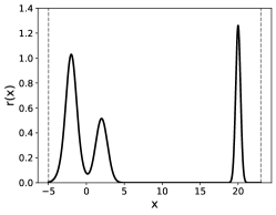
We consider a one-dimensional line environment, with state space , where indexes the position of a state in a trajectory. The source state is and trajectories terminate after exactly steps. The terminal states are therefore . The reward density, plotted in Figure 1, consists of an asymmetric bimodal peak near the origin and an additional distant lone peak. It is given by the Gaussian mixture distribution:
| (2) |
where is a Gaussian density with mean and variance . The forward and backward probability transition kernels are a mixture of Gaussian distributions which, along with the flow , are parameterised by an MLP.
We compare the following exploration strategies: entirely on-policy (no exploration), noisy exploration, Thompson Sampling, and MetaGFN. For each strategy, we use a replay buffer and alternate between an exploration batch and a replay buffer batch. For MetaGFN, we use , and always regenerate MetaGFN training trajectories using the current backward policy. As the environment is one-dimensional, the collective variable is simply . We evaluate performance by computing the L1 error between the known reward distribution and the empirical on-policy distribution during training (see Appendix E.1 for the full experimental details).
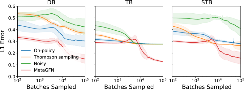
The results (mean and standard deviation over random seeds) for each loss function and exploration strategy are shown in Figure 2. Among the three loss functions, TB loss has the lowest variance loss profiles, and MetaGFN consistently converges to a lower minimum error than all other exploration strategies. Indeed, MetaGFN was the only method that consistently sampled the distant reward peak at , while other methods plateau in error after locking onto the central modes (Appendix E.2). Despite this, we observed that in the initial stages of training, all exploration strategies found occasional samples from the distant peak. The reason MetaGFN is the only method that converges is that Adaptive Metadynamics manages to consistently sample the distant peak, even if the on-policy starts to focus on the central modes. This keeps the replay buffer populated with samples from every reward peak during training, which eventually encourages the on-policy to sample from every mode. The small increase in the loss of MetaGFN around batch number happens because the on-policy distribution widens when Adaptive Metadynamics first discovers the distant peak. In Appendix E.2, we show further details of Adaptive Metadynamics in this environment and we compare different MetaGFN variants, with and without noise, and with and without trajectory regeneration. We confirm that the version of MetaGFN presented in Figure 2 (no added noise and always regenerate trajectories) is the most robust variant.
4.2 Grid environment
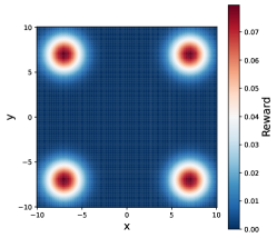
We consider a two-dimensional environment, with state space . The source state is and trajectories terminate after exactly steps. Terminal states are . The reward function is given by the sum of four symmetric Gaussians with means and variances (Figure 3). The forward and backward probability transition kernels are a mixture of bivariate Gaussian distributions with means and diagonal variance matrices, along with the flow , parameterised by an MLP. We consider the same exploration strategies and evaluation measures as for the Line Environment (see Appendix F for full experiment details).
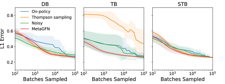
The results (mean and standard deviation over random seeds) for each loss function and exploration strategy are shown in Figure 4. We see that for most loss functions and exploration strategies (except Thompson sampling with TB loss), the training curves converge to a low loss, indicating that all four modes of the grid environment are well-sampled. However, in all cases, MetaGFN converges faster than other exploration strategies. The fastest convergence occurs for MetaGFN with TB loss; after batches MetaGFN has reached a similar loss that noisy exploration reaches after batches and on-policy reaches after batches. Meanwhile, the loss curves have lower error indicating more stable training with MetaGFN in this environment.
4.3 Alanine dipeptide environment
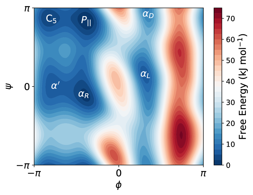
One application of continuous GFlowNets is molecular conformation sampling Volokhova et al. (2023). Here, we train a GFlowNet to sample conformational states of alanine dipeptide (AD), a small biomolecule of atoms that plays a key role in modelling backbone dynamics of proteins Hermans (2011). The metastable states of AD can be distinguished in a two-dimensional CV space of and , the two backbone dihedral angles. The resulting free energy surface for AD in explicit water, , obtained after extensive sampling long molecular dynamics simulation is shown in Figure 5(a). The metastable states (energy minima), in increasing energy, are , , , , and .
The state space is . The source state is and trajectories terminate after exactly steps. Terminal states are . The reward density is given by the Boltzmann weight, , where is the normalisation constant. The forward and backward probability transition kernels are defined as a mixture of bivariate von Mises distributions, parameterised through an MLP. We consider the same exploration strategies and evaluation measures as for the Line Environment (see Appendix G for full experimental details).
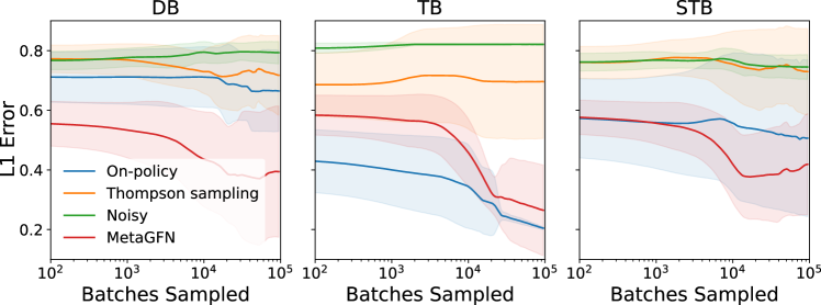
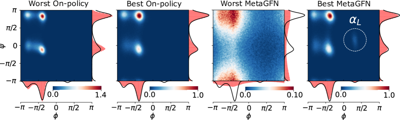
The results (mean and standard deviation over random seeds) for each loss function and exploration strategy are shown in Figure 6. For each loss function, models trained with MetaGFN generally converge to a lower minimum error than all other exploration strategies. For TB loss, however, the average L1 error is marginally higher than on-policy training, but this conceals the fact that the best-case error is smaller. Thus, to better understand this result, we examine the best and worst training runs (as measured by L1 error) for TB on-policy and TB MetaGFN, shown in Figure 7. We see that the best run trained with metadynamics can sample from the rare minima, unlike the on-policy run. In the worst run, MetaGFN fails to converge (although this is rare; only one of 10 runs failed). In Table 1, we quantify how often the different AD modes were correctly sampled over the different repeats (a mode is correctly sampled if the on-policy distribution also has a mode within the correct basin of attraction). The only mode not correctly sampled by any method is , which has a natural abundance approximately times less frequent than . We see that TB loss with MetaGFN is the only combination that can consistently sample the majority of modes, whilst noisy exploration and Thompson Sampling both perform worse than on-policy in this environment.
| DB | STB | TB | ||||
|---|---|---|---|---|---|---|
| OP | MD | OP | MD | OP | MD | |
| 1 | 7 | 6 | 5 | 10 | 8 | |
| 6 | 9 | 7 | 10 | 10 | 9 | |
| 2 | 7 | 5 | 6 | 10 | 8 | |
| 6 | 9 | 5 | 10 | 5 | 9 | |
| 0 | 1 | 1 | 0 | 0 | 8 | |
5 Limitations
For metadynamics to be an effective sampler, the CVs must be low-dimensional and bounded, properties that were satisfied in both our experimental environments. Therefore, it is necessary to either know such CVs in advance, assuming they exist or learn them automatically from data Sidky et al. (2020). An alternative approach would be to learn CVs adaptively by parameterising the CV function by a neural network and updating its parameters by back-propagating through the GFlowNet loss when training on MetaGFN trajectories. A final improvement could be to replace the metadynamics algorithm itself with a variant with smoother convergence properties, such as well-tempered metadynamics Barducci et al. (2008) or on-the-fly probability enhanced sampling (OPES) Invernizzi (2021). We leave these extensions for future work.
6 Conclusions
While exploration strategies for discrete Generative Flow Networks (GFlowNets) have received extensive attention, the methodologies for continuous GFlowNets remain relatively underexplored. To address this gap, we illustrated how metadynamics, a widely used enhanced sampling technique in molecular dynamics, can be adapted as an effective exploration strategy for continuous GFlowNets.
In molecular dynamics, atomic forces can be computed as the gradient of the potential, whereas continuous GFlowNets tackle problems where the reward function is a black box and gradients are inaccessible. We demonstrated how the method could be adapted by updating a kernel density estimate of the reward function on-the-fly, and proved that this is guaranteed to explore the space in an appropriate limit. Our empirical investigations show that MetaGFN offers a computationally efficient means to explore new modes in environments where prior knowledge of collective variables exists. Importantly, this work advocates an approach wherein techniques derived from molecular modelling can be adapted for machine learning tasks. Looking ahead, we anticipate that this could be a fruitful area of cross-disciplinary research, where existing ideas from the enhanced sampling literature can find applications in a broad range of generative modelling and reinforcement learning tasks.
References
- Barducci et al. [2008] Alessandro Barducci, Giovanni Bussi, and Michele Parrinello. Well-Tempered Metadynamics: A Smoothly Converging and Tunable Free-Energy Method. Physical Review Letters, 100(2):020603, January 2008. ISSN 0031-9007, 1079-7114. doi: 10.1103/PhysRevLett.100.020603. URL https://link.aps.org/doi/10.1103/PhysRevLett.100.020603.
- Bengio et al. [2021a] Emmanuel Bengio, Moksh Jain, Maksym Korablyov, Doina Precup, and Y. Bengio. Flow Network based Generative Models for Non-Iterative Diverse Candidate Generation. ArXiv, June 2021a.
- Bengio et al. [2021b] Yoshua Bengio, T. Deleu, J. E. Hu, Salem Lahlou, Mo Tiwari, and Emmanuel Bengio. GFlowNet Foundations. ArXiv, November 2021b.
- Bonomi et al. [2019] Massimiliano Bonomi, Giovanni Bussi, Carlo Camilloni, Gareth A. Tribello, Pavel Banáš, Alessandro Barducci, Mattia Bernetti, Peter G. Bolhuis, Sandro Bottaro, Davide Branduardi, Riccardo Capelli, Paolo Carloni, Michele Ceriotti, Andrea Cesari, Haochuan Chen, Wei Chen, Francesco Colizzi, Sandip De, Marco De La Pierre, Davide Donadio, Viktor Drobot, Bernd Ensing, Andrew L. Ferguson, Marta Filizola, James S. Fraser, Haohao Fu, Piero Gasparotto, Francesco Luigi Gervasio, Federico Giberti, Alejandro Gil-Ley, Toni Giorgino, Gabriella T. Heller, Glen M. Hocky, Marcella Iannuzzi, Michele Invernizzi, Kim E. Jelfs, Alexander Jussupow, Evgeny Kirilin, Alessandro Laio, Vittorio Limongelli, Kresten Lindorff-Larsen, Thomas Löhr, Fabrizio Marinelli, Layla Martin-Samos, Matteo Masetti, Ralf Meyer, Angelos Michaelides, Carla Molteni, Tetsuya Morishita, Marco Nava, and The PLUMED consortium. Promoting transparency and reproducibility in enhanced molecular simulations. Nature Methods, 16(8):670–673, August 2019. ISSN 1548-7091. doi: 10.1038/s41592-019-0506-8.
- Bortolussi and Policriti [2008] Luca Bortolussi and Alberto Policriti. Hybrid Systems and Biology. In Marco Bernardo, Pierpaolo Degano, and Gianluigi Zavattaro, editors, Formal Methods for Computational Systems Biology, pages 424–448, Berlin, Heidelberg, 2008. Springer Berlin Heidelberg. ISBN 978-3-540-68894-5.
- Bussi and Laio [2020] Giovanni Bussi and Alessandro Laio. Using metadynamics to explore complex free-energy landscapes. Nature Reviews Physics, 2:200–212, March 2020. doi: 10.1038/s42254-020-0153-0. URL https://ui.adsabs.harvard.edu/abs/2020NatRP...2..200B. ADS Bibcode: 2020NatRP…2..200B.
- Cipcigan et al. [2023] Flaviu Cipcigan, Jonathan Booth, Rodrigo Neumann Barros Ferreira, Carine Ribeiro dos Santos, and Mathias Steiner. Discovery of Novel Reticular Materials for Carbon Dioxide Capture using GFlowNets, October 2023. URL http://arxiv.org/abs/2310.07671. arXiv:2310.07671 [cond-mat].
- De Vivo et al. [2016] Marco De Vivo, Matteo Masetti, Giovanni Bottegoni, and Andrea Cavalli. Role of Molecular Dynamics and Related Methods in Drug Discovery. Journal of Medicinal Chemistry, 59(9):4035–4061, May 2016. ISSN 0022-2623. doi: 10.1021/acs.jmedchem.5b01684. URL https://doi.org/10.1021/acs.jmedchem.5b01684. Publisher: American Chemical Society.
- Deleu et al. [2022] Tristan Deleu, António Góis, Chris Emezue, Mansi Rankawat, Simon Lacoste-Julien, Stefan Bauer, and Yoshua Bengio. Bayesian Structure Learning with Generative Flow Networks, June 2022. URL http://arxiv.org/abs/2202.13903. arXiv:2202.13903 [cs, stat].
- Eastman et al. [2017] Peter Eastman, Jason Swails, John D. Chodera, Robert T. McGibbon, Yutong Zhao, Kyle A. Beauchamp, Lee-Ping Wang, Andrew C. Simmonett, Matthew P. Harrigan, Chaya D. Stern, Rafal P. Wiewiora, Bernard R. Brooks, and Vijay S. Pande. OpenMM 7: Rapid development of high performance algorithms for molecular dynamics. PLoS computational biology, 13(7):e1005659, July 2017. ISSN 1553-7358. doi: 10.1371/journal.pcbi.1005659.
- Hawkins [2017] Paul C. D. Hawkins. Conformation Generation: The State of the Art. Journal of Chemical Information and Modeling, 57(8):1747–1756, August 2017. ISSN 1549-9596. doi: 10.1021/acs.jcim.7b00221. URL https://doi.org/10.1021/acs.jcim.7b00221. Publisher: American Chemical Society.
- Hermans [2011] Jan Hermans. The amino acid dipeptide: Small but still influential after 50 years. Proceedings of the National Academy of Sciences, 108(8):3095–3096, February 2011. doi: 10.1073/pnas.1019470108. URL https://www.pnas.org/doi/full/10.1073/pnas.1019470108. Publisher: Proceedings of the National Academy of Sciences.
- Hu et al. [2023] Edward J. Hu, Nikolay Malkin, Moksh Jain, Katie Everett, Alexandros Graikos, and Yoshua Bengio. GFlowNet-EM for learning compositional latent variable models, June 2023. URL http://arxiv.org/abs/2302.06576. arXiv:2302.06576 [cs, stat].
- Invernizzi [2021] Michele Invernizzi. OPES: On-the-fly Probability Enhanced Sampling Method. Il Nuovo Cimento C, 44(405):1–4, September 2021. ISSN 03905551, 03905551. doi: 10.1393/ncc/i2021-21112-8. URL http://arxiv.org/abs/2101.06991. arXiv:2101.06991 [physics].
- Jain et al. [2022] Moksh Jain, Emmanuel Bengio, Alex Hernandez-Garcia, Jarrid Rector-Brooks, Bonaventure F. P. Dossou, Chanakya Ajit Ekbote, Jie Fu, Tianyu Zhang, Michael Kilgour, Dinghuai Zhang, Lena Simine, Payel Das, and Yoshua Bengio. Biological Sequence Design with GFlowNets. In Proceedings of the 39th International Conference on Machine Learning, pages 9786–9801. PMLR, June 2022. URL https://proceedings.mlr.press/v162/jain22a.html. ISSN: 2640-3498.
- Jain et al. [2023] Moksh Jain, Sharath Chandra Raparthy, Alex Hernandez-Garcia, Jarrid Rector-Brooks, Yoshua Bengio, Santiago Miret, and Emmanuel Bengio. Multi-Objective GFlowNets, July 2023. URL http://arxiv.org/abs/2210.12765. arXiv:2210.12765 [cs, stat].
- Jorgensen et al. [1983] William L. Jorgensen, Jayaraman Chandrasekhar, Jeffry D. Madura, Roger W. Impey, and Michael L. Klein. Comparison of simple potential functions for simulating liquid water. The Journal of Chemical Physics, 79(2):926–935, July 1983. ISSN 0021-9606. doi: 10.1063/1.445869. URL https://doi.org/10.1063/1.445869.
- Kim et al. [2024] Minsu Kim, Taeyoung Yun, Emmanuel Bengio, Dinghuai Zhang, Yoshua Bengio, Sungsoo Ahn, and Jinkyoo Park. Local Search GFlowNets, March 2024. URL http://arxiv.org/abs/2310.02710. arXiv:2310.02710 [cs, stat].
- Lahlou et al. [2023] Salem Lahlou, Tristan Deleu, Pablo Lemos, Dinghuai Zhang, Alexandra Volokhova, Alex Hernández-García, Léna Néhale Ezzine, Yoshua Bengio, and Nikolay Malkin. A theory of continuous generative flow networks. Proceedings of the 40th International Conference on Machine Learning, 2023. doi: 10.48550/ARXIV.2301.12594. URL https://arxiv.org/abs/2301.12594. Publisher: arXiv Version Number: 2.
- Laio and Gervasio [2008] Alessandro Laio and Francesco L. Gervasio. Metadynamics: a method to simulate rare events and reconstruct the free energy in biophysics, chemistry and material science. Reports on Progress in Physics, 71(12):126601, November 2008. ISSN 0034-4885. doi: 10.1088/0034-4885/71/12/126601. URL https://dx.doi.org/10.1088/0034-4885/71/12/126601.
- Laio and Parrinello [2002] Alessandro Laio and Michele Parrinello. Escaping free-energy minima. Proceedings of the National Academy of Sciences, 99(20):12562–12566, October 2002. doi: 10.1073/pnas.202427399. URL https://www.pnas.org/doi/full/10.1073/pnas.202427399. Publisher: Proceedings of the National Academy of Sciences.
- Luo et al. [2024] Shuang Luo, Yinchuan Li, Shunyu Liu, Xu Zhang, Yunfeng Shao, and Chao Wu. Multi-agent Continuous Control with Generative Flow Networks. Neural Networks, 174:106243, June 2024. ISSN 0893-6080. doi: 10.1016/j.neunet.2024.106243. URL https://www.sciencedirect.com/science/article/pii/S0893608024001679.
- Madan et al. [2022] Kanika Madan, Jarrid Rector-Brooks, Maksym Korablyov, Emmanuel Bengio, Moksh Jain, Andrei Nica, Tom Bosc, Yoshua Bengio, and Nikolay Malkin. Learning GFlowNets from partial episodes for improved convergence and stability. Proceedings of the 40th International Conference on Machine Learning, 2022. doi: 10.48550/ARXIV.2209.12782. URL https://arxiv.org/abs/2209.12782. Version Number: 3.
- Malkin et al. [2022] Nikolay Malkin, Moksh Jain, Emmanuel Bengio, Chen Sun, and Y. Bengio. Trajectory Balance: Improved Credit Assignment in GFlowNets. ArXiv, January 2022.
- Malkin et al. [2023] Nikolay Malkin, Salem Lahlou, Tristan Deleu, Xu Ji, Edward Hu, Katie Everett, Dinghuai Zhang, and Yoshua Bengio. GFlowNets and variational inference, March 2023. URL http://arxiv.org/abs/2210.00580. arXiv:2210.00580 [cs, stat].
- Neunert et al. [2020] Michael Neunert, Abbas Abdolmaleki, Markus Wulfmeier, Thomas Lampe, Tobias Springenberg, Roland Hafner, Francesco Romano, Jonas Buchli, Nicolas Heess, and Martin Riedmiller. Continuous-Discrete Reinforcement Learning for Hybrid Control in Robotics. In Proceedings of the Conference on Robot Learning, pages 735–751. PMLR, May 2020. URL https://proceedings.mlr.press/v100/neunert20a.html. ISSN: 2640-3498.
- Nummelin [1984] Esa Nummelin. General Irreducible Markov Chains and Non-Negative Operators. Cambridge Tracts in Mathematics. Cambridge University Press, Cambridge, 1984. ISBN 978-0-521-60494-9. doi: 10.1017/CBO9780511526237. URL https://www.cambridge.org/core/books/general-irreducible-markov-chains-and-nonnegative-operators/0557D49C011AA90B761FC854D5C14983.
- Pan et al. [2022] Ling Pan, Dinghuai Zhang, Aaron Courville, Longbo Huang, and Yoshua Bengio. Generative Augmented Flow Networks, October 2022. URL http://arxiv.org/abs/2210.03308. arXiv:2210.03308 [cs].
- Pavliotis [2014] Grigorios A. Pavliotis. Stochastic Processes and Applications: Diffusion Processes, the Fokker-Planck and Langevin Equations, volume 60 of Texts in Applied Mathematics. Springer, New York, NY, 2014. ISBN 978-1-4939-1322-0. doi: 10.1007/978-1-4939-1323-7. URL https://link.springer.com/10.1007/978-1-4939-1323-7.
- Rector-Brooks et al. [2023] Jarrid Rector-Brooks, Kanika Madan, Moksh Jain, Maksym Korablyov, Cheng-Hao Liu, Sarath Chandar, Nikolay Malkin, and Yoshua Bengio. Thompson sampling for improved exploration in GFlowNets, June 2023. URL http://arxiv.org/abs/2306.17693. arXiv:2306.17693 [cs].
- Salomon-Ferrer et al. [2013] Romelia Salomon-Ferrer, David A. Case, and Ross C. Walker. An overview of the Amber biomolecular simulation package. WIREs Computational Molecular Science, 3(2):198–210, 2013. ISSN 1759-0884. doi: 10.1002/wcms.1121. URL https://onlinelibrary.wiley.com/doi/abs/10.1002/wcms.1121. _eprint: https://onlinelibrary.wiley.com/doi/pdf/10.1002/wcms.1121.
- Shahriari et al. [2016] Bobak Shahriari, Kevin Swersky, Ziyu Wang, Ryan P. Adams, and Nando De Freitas. Taking the Human Out of the Loop: A Review of Bayesian Optimization. Proceedings of the IEEE, 104(1):148–175, January 2016. ISSN 0018-9219, 1558-2256. doi: 10.1109/JPROC.2015.2494218. URL https://ieeexplore.ieee.org/document/7352306/.
- Shen et al. [2023a] Max W. Shen, Emmanuel Bengio, Ehsan Hajiramezanali, Andreas Loukas, Kyunghyun Cho, and Tommaso Biancalani. Towards Understanding and Improving GFlowNet Training. Proceedings of the 40th International Conference on Machine Learning, 2023a. doi: 10.48550/ARXIV.2305.07170. URL https://arxiv.org/abs/2305.07170. Publisher: arXiv Version Number: 1.
- Shen et al. [2023b] Tony Shen, Mohit Pandey, Jason Smith, Artem Cherkasov, and Martin Ester. TacoGFN: Target Conditioned GFlowNet for Structure-Based Drug Design, December 2023b. URL http://arxiv.org/abs/2310.03223. arXiv:2310.03223 [cs].
- Sidky et al. [2020] Hythem Sidky, Wei Chen, and Andrew L. Ferguson. Machine learning for collective variable discovery and enhanced sampling in biomolecular simulation. Molecular Physics, 118(5), March 2020. ISSN 0026-8976. doi: 10.1080/00268976.2020.1737742. URL https://www.osti.gov/pages/biblio/1651117. Institution: Argonne National Laboratory (ANL), Argonne, IL (United States) Publisher: Taylor & Francis.
- Swiler et al. [2012] Laura Painton Swiler, Patricia Diane Hough, Peter Qian, Xu Xu, Curtis B. Storlie, and Herbert K. H. Lee. Surrogate models for mixed discrete-continuous variables. Technical Report SAND2012-0491, Sandia National Laboratories (SNL), Albuquerque, NM, and Livermore, CA (United States), August 2012. URL https://www.osti.gov/biblio/1055621.
- Volokhova et al. [2023] Alexandra Volokhova, Michał Koziarski, Alex Hernández-García, Cheng-Hao Liu, Santiago Miret, Pablo Lemos, Luca Thiede, Zichao Yan, Alán Aspuru-Guzik, and Yoshua Bengio. Towards equilibrium molecular conformation generation with GFlowNets, October 2023. URL http://arxiv.org/abs/2310.14782. arXiv:2310.14782 [cs].
- Yang et al. [2019] Yi Isaac Yang, Qiang Shao, Jun Zhang, Lijiang Yang, and Yi Qin Gao. Enhanced sampling in molecular dynamics. The Journal of Chemical Physics, 151(7):070902, August 2019. ISSN 0021-9606. doi: 10.1063/1.5109531. URL https://doi.org/10.1063/1.5109531.
- Zhang et al. [2023] David W. Zhang, Corrado Rainone, Markus Peschl, and Roberto Bondesan. Robust Scheduling with GFlowNets, February 2023. URL http://arxiv.org/abs/2302.05446. arXiv:2302.05446 [cs].
- Zhang et al. [2022] Dinghuai Zhang, Nikolay Malkin, Zhen Liu, Alexandra Volokhova, Aaron Courville, and Yoshua Bengio. Generative Flow Networks for Discrete Probabilistic Modeling. In Proceedings of the 39th International Conference on Machine Learning, pages 26412–26428. PMLR, June 2022. URL https://proceedings.mlr.press/v162/zhang22v.html. ISSN: 2640-3498.
Appendix A Loss functions
For a complete trajectory , the detailed balanced loss (DB) is
where is replaced with if is terminal.
The subtrajectory balance loss (STB) is
where is replaced with if is terminal. In the above, is a hyperparameter. The limit leads to average detailed balance. The limit gives the trajectory balance objective. We use in our experiments.
Appendix B Langevin dynamics
Langevin dynamics (LD), is defined through the Stochastic Differential Equation (SDE):
| (3) | |||
| (4) |
In the above, are vectors of instantaneous position and momenta respectively, is a force function, is a vector of independent Wiener processes, is a constant diagonal mass matrix, and are constant scalars which can be interpreted as a friction coefficient and inverse temperature respectively. In conventional Langevin dynamics, the force function is given by the gradient of the potential energy function, , where and the dynamics are ergodic with respect to the Gibbs-Boltzmann density
where is the Hamiltonian. Since the Hamiltonian is separable in position and momenta terms, the marginal Gibbs-Boltzmann density is position space is simply .
Appendix C Proofs
Lemma C.1.
Let and be sequences of real functions where , and . Then, for all , we have .
Proof.
and the right-hand side is the product of two functions whose limit exists so, by the product rule of limits
so done. ∎
Lemma C.2.
Let be a sequence of continuous random variables that take values on a bounded domain that asymptotically approaches the uniform random variable on , i.e. uniformly. Further, suppose
exists, where is a sample from and and are analytic functions on and respectively. Then,
where the are samples from . We make no assumption of independence of samples.
Proof.
Fix a probability space on which and are defined. Recall that a continuous random variable that takes values on is a measurable function where is a measure space and is the Borel -algebra on . Let denote an arbitrary element of the sample space. The requirement that uniformly can be written formally as:
We prove the Lemma by showing that equality holds for all possible sequences of outcomes . That is, we prove:
| (5) |
Since these are ratios of infinite series, to prove their equality it is sufficient to show that the numerator of the LHS is asymptotically equivalent to the numerator of the RHS and that the denominator of the LHS is asymptotically equivalent to the denominator of the RHS. Recall that two sequences of real functions and are asymptotically equivalent if where is a constant. First, we prove that this holds with
| (6) |
and
| (7) |
We write
Dividing by and taking the limit we have
Since and are analytic and for all terms in the sums we have, by Taylor expansion, and , hence
Finally, since can be made arbitrarily small by partitioning the sum at a that is sufficiently large, we conclude that , hence and as defined in (6) and (7) are asymptotically equivalent. By a similar argument, it can be shown that
and
are also asymptotically equivalent. This proves (5).
∎
Below, we present the proof of Theorem 3.1 that appears in the main text.
Proof.
For concreteness, throughout this proof we assume that the kernel function is a Gaussian. We explain at the appropriate stage in the proof, indicated by (*), how this assumption can be relaxed.
First we take the limit. Since the log function is continuous, the limit and log can be interchanged and we have
Recall the uniform time discretisation of metadynamics (Algorithm 1). Thus, we can write
| (8) |
| (9) |
Since the domain is bounded, we know that for fixed , both (8) and (9) have limit at infinity, i.e. and . Hence, by Lemma C.1, we have
provided the limit on the RHS exists. Next, we show that this limit exists by computing it explicitly. The limit can be written
Recall that metadynamics eventually leads to uniform sampling over the domain, independent of the potential. Hence, since and are analytic, by Lemma C.2 we may replace the metadynamics samples with samples from a uniform distribution, denoted :
In the limit, the ratio of sums with uniform sampling becomes a ratio of integrals:
where is the domain. The limit is therefore a (scaled) convolution of the reward function with a Gaussian in the collective variable space with width vector . Taking the limit for all , the Gaussian convergences to a delta distribution in the collective variable space and we have
(*) This step also holds for any kernel that becomes distributionally equivalent to a Dirac delta function in the limit that its variance parameter goes to zero. In particular, it also holds for the von Mises distribution that we use in our alanine dipeptide experiment in .
Finally, we take the limit to obtain
| (10) | ||||
| (11) | ||||
| (12) |
where we have used the definition and in the last step we used the definition of the marginal potential energy in the collective variable space. If is invertible, then the delta function simplifies to a delta function in the original space and we obtain the original potential instead of the marginal potential. ∎
Appendix D Algorithms
In the algorithm below, we present the variant of MetaGFN where we store Adaptive Metadynamics samples in the replay buffer and regenerate trajectories using the current backward policy when retrieving from the replay buffer. This is the variant we used in our experiments in the main text.
Appendix E Experiment details: line environment
E.1 Experimental setup
Parameterisation We parameterise , and the flow through an MLP with 3 hidden layers, 256 hidden units per layer. We use the GELU activation function and dropout probability after each layer. This defines the torso of the MLP. Connecting from this common torso, the MLP has three single-layer, fully connected heads. The first two heads have output dimension and parameterise the means (), standard deviations () and weights () of the mixture of Gaussians for the forward and backward policies respectively. The third head has output dimension and parameterises the flow function . The mean and standard deviation outputs are passed through a sigmoid function and transformed so that they map to the ranges and . The mixture weights are normalised with the softmax function. The exception to this parameterisation is the backward transition to the source state which is fixed to be the Dirac delta distribution centred on the source, i.e. . For the TB loss, we treat as a separate learnable parameter.
Replay buffer The replay buffer has capacity for trajectories. Trajectories are stored in the replay buffer only if the terminal state’s reward exceeds . When drawing a replay buffer batch, trajectories are bias-sampled: randomly drawn from the upper of trajectories with the highest rewards, and the remaining randomly drawn from the lower .
Noisy exploration Noisy exploration is defined by adding an additional constant, , to the standard deviations of the Gaussian distributions of the forward and backward policies. Specifically, the forward policy becomes , and similarly for the backward policy. We schedule the value of so that it decreases during training according to an exponential-flat schedule:
| (13) |
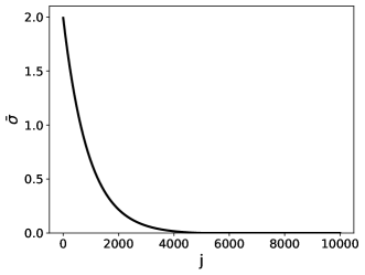
where is the batch number and is the initial noise, plotted in Figure 8.
Thompson Sampling We use heads with the bootstrapping probability parameter set to .
MetaGFN We use , , , , , , . The domain of Adaptive Metadynamics is restricted to and reflection conditions are imposed at the boundary. The bias and KDE potentials are stored on a uniform grid with grid spacing . Initial metadynamics samples are drawn from a Gaussian distribution, mean and variance , and initial momenta from a Gaussian distribution, mean and variance .
Training parameters In all experiments, we use batch size and for batches. We use a learning rate with a linear schedule, starting at and finishing at . For the TB loss, we train the with a higher initial learning rate of (also linearly scheduled). For the STB loss, we use , a value that has worked well in the discrete setting Madan et al. [2022]. We use the Adam optimiser with gradient clipping. For all loss functions, we clip the minimum log-reward signal at . This enables the model to learn despite regions of near-zero reward between the modes of .
Evaluation The L1 error between the known reward distribution, , and the empirical on-policy distribution, denoted , estimated by sampling on-policy trajectories and computing the empirical distribution over terminal states. Specifically, we compute
| (14) |
where the integral is estimated by a discrete sum with grid spacing . Note that this error is normalised such that for all valid probability distributions , we have .
Compute resources Experiments are performed in PyTorch on a desktop with 32Gb of RAM and a 12-core 2.60GHz i7-10750H CPU. It takes approximately hour to train a continuous GFlowNet in this environment with batches. The additional computational expense of running Adaptive Metadynamics was negligible compared to the training time of the models.
E.2 Results
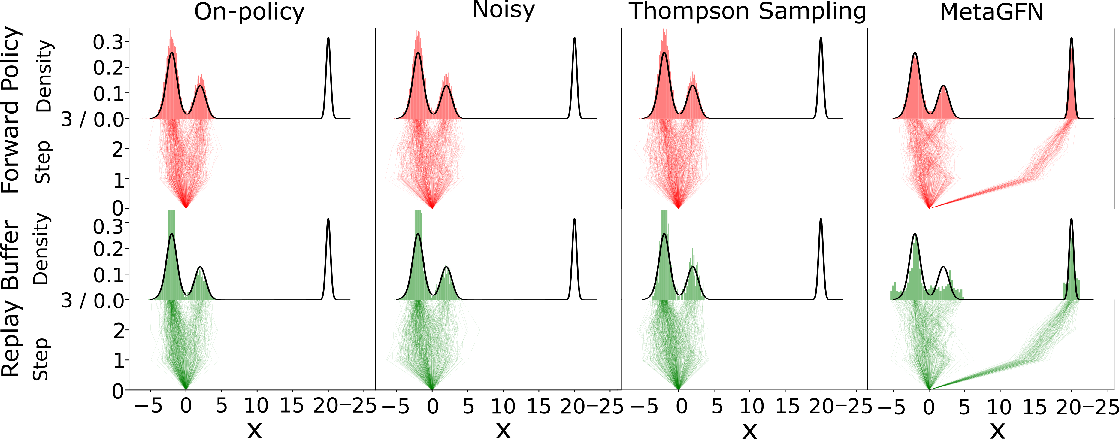
On-policy distributions Figure 9 shows the forward policy and replay buffer distributions (with bias sampling) after training for iterations with TB loss. MetaGFN is the only method that can uniformly populate the replay buffer and consistently learn all three peaks.
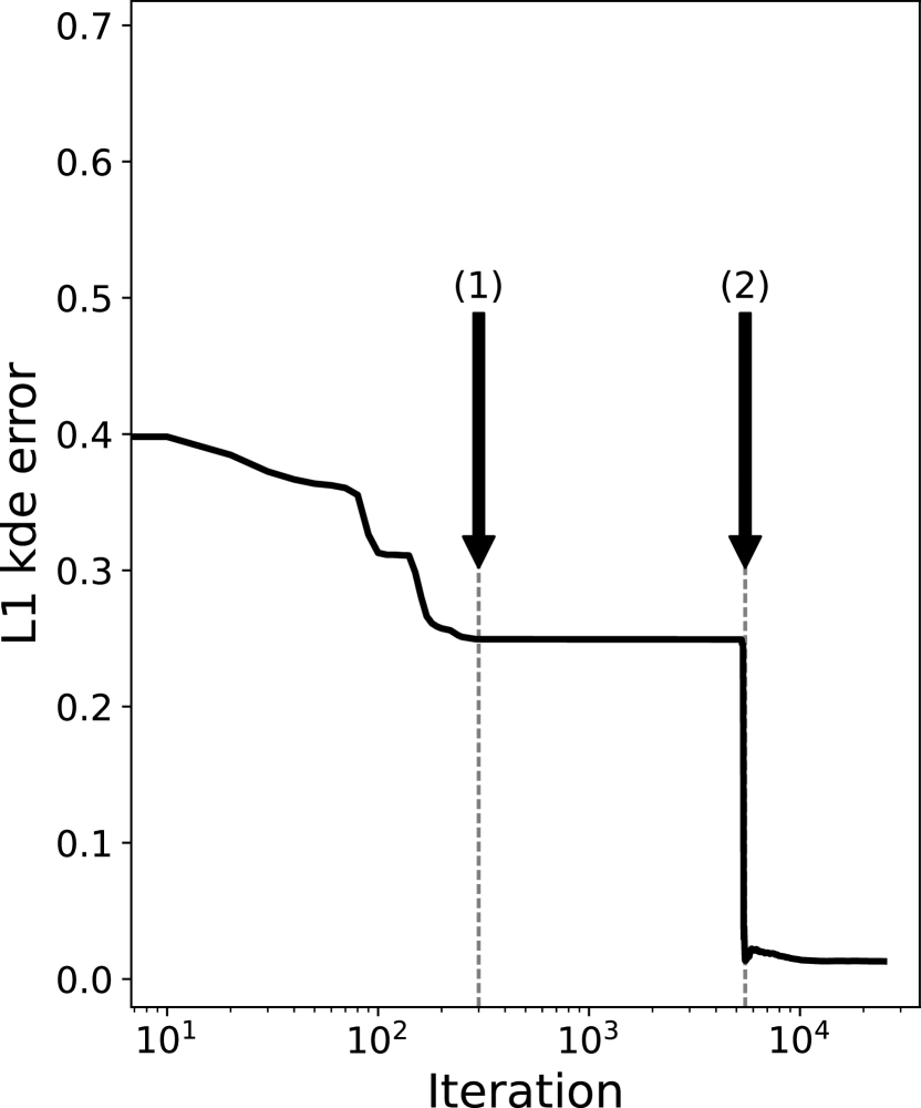
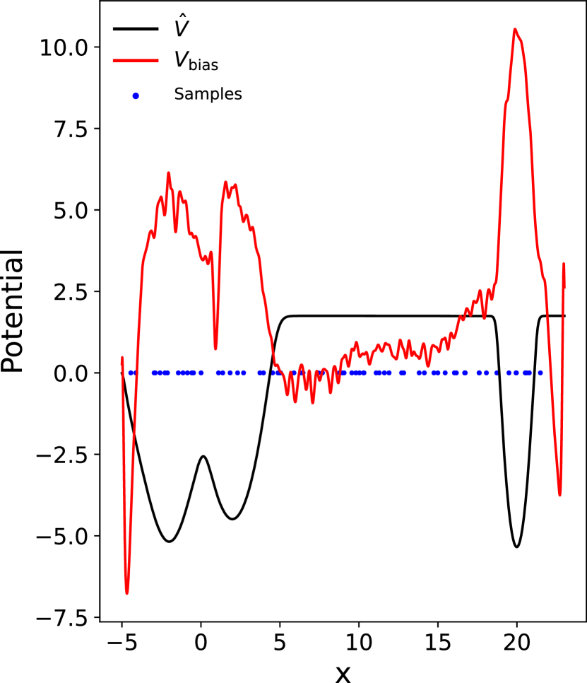
Adaptive Metadynamics Figure 10(a) shows the L1 error between the density implied by the KDE potential and the true reward distribution during a typical training run. Figure 10(b) shows the resulting and at the end of the training. By (1), Adaptive Metadynamics has fully explored the central peaks. At (2), the third peak is discovered, prompting rapid adjustment of the KDE potential. By iterations, a steady state is reached and the algorithm is sampling the domain uniformly.
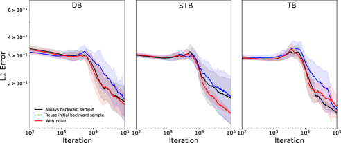
Comparing MetaGFN Variants We consider three MetaGFN variants. The first variant, always backwards sample, regenerates the entire trajectory using the current backward policy when pulling from the replay buffer. The second variant, reuse initial backwards sample, generates the trajectory when first added to the replay buffer and reuses the entire trajectory if subsequently sampled. The third variant, with noise, is to always backwards sample with noisy exploration as per equation (13). We plot the L1 policy errors in Figure 11. We observe that always backward sample is better than reuse initial backwards sample for all loss functions. For DB and TB losses, there is no evidence of any benefit of adding noise, whereas noise improves training for STB loss, performing very similarly to TB loss without noise.
Appendix F Experiment details: grid environment
Parameterisation We parameterise , and the flow through an MLP with 3 hidden layers, 512 hidden units per layer, GELU activation function and dropout probability , similar to the Line Environment. The first two heads have output dimension and parameterise the means, standard deviations and weights of the mixture of bivariate Gaussians. The third head has output dimension and parameterises the flow function . The means and standard deviations are mapped to the range and through sigmoid functions. Mixture weights are normalised with the softmax function.
Replay buffer Identical to the Line Environment replay buffer, except trajectories are only stored when the terminal state’s reward exceeds .
Noisy exploration We use the same noise profile as the Line Environment, equation (13). The noise is added equally to both dimensions of the standard deviation.
Thompson sampling We use heads with the bootstrap probability parameter set to .
MetaGFN We use , , , , , , , . The bias and KDE potentials are stored on a uniform grid with grid spacing . Initial samples are drawn from a Gaussian distribution, mean centred , variance . Momenta are initialised to zero.
Training parameters The same as for the Line Environment, see Appendix E.1.
Evaluation The L1 error between the histogram of the terminal states of on-policy samples and the exact distribution is computed. , estimated by a discrete sum with grid spacing .
Compute resources Experiments are performed in PyTorch on a desktop with 32Gb of RAM and a 12-core 2.60GHz i7-10750H CPU. It takes approximately hours to train a continuous GFlowNet in this environment with batches. The additional computational expense of running Adaptive Metadynamics is less than .
Appendix G Experiment details: alanine dipeptide environment
Computing the Free Energy Surface To obtain a ground-truth free energy surface (FES) in - space, we ran a 250ns NPT well-tempered metadynamics MD simulation of alanine dipeptide at temperature 300K (), pressure 1bar with the TIP3P explicit water model Jorgensen et al. [1983]. We used the PLUMMED plugin Bonomi et al. [2019] for OpenMM Eastman et al. [2017] with the AMBER14 force field Salomon-Ferrer et al. [2013].
Parameterisation We parameterise , and through three heads of an MLP with 3 hidden layers with 512 hidden units per layer, with GeLU activations and dropout probability , similar to the Line Environment. The first two heads have output dimensions of , parameterising the means, concentrations, and weights of the mixture of von Mises policy. The third head has output dimension and parameterises the flow function . The means are mapped to the range through . Concentrations are parameterised in log space and passed through a sigmoid to map to the range . Mixture weights are normalised with the softmax function.
Replay buffer The replay buffer has capacity for trajectories. Trajectories are stored in the replay buffer only if the terminal state’s reward exceeds . When drawing a replay buffer batch, trajectories are bias-sampled: randomly drawn from the upper of trajectories with the highest rewards, and the remaining randomly drawn from the lower .
Noisy exploration We use the same noise profile as the Line Environment, equation (13). The noise is now added to the concentration parameter . Concentration is related to standard deviation through .
Thompson Sampling We use 10 heads with the bootstrap probability parameter set to 0.3.
MetaGFN We use , , , , , , , , . The bias and KDE potentials are stored on a uniform grid with grid spacing . Initial samples are drawn from a Gaussian distribution, mean centred , variance , and initial momenta from a Gaussian, mean , variance .
Training parameters The same as for the Line Environment, see Appendix E.1.
Evaluation The L1 error of a histogram of on-policy samples, , is computed via a two-dimensional generalisation of (14); , estimated by a discrete sum with grid spacing .
Compute resources Experiments are performed in PyTorch on a desktop with 32Gb of RAM and a 12-core 2.60GHz i7-10750H CPU. It takes approximately hours to train a continuous GFlowNet in this environment with batches. The additional computational expense of running Adaptive Metadynamics was less than .