Asymmetry Amplification by a Nonadiabatic Passage through a Critical Point

Abstract

We propose and solve a minimal model of dynamic passage through a quantum second order phase transition in the presence of weak symmetry breaking interactions and no dissipation. The evolution eventually leads to a highly asymmetric state, no matter how weak the symmetry breaking term is. This suggests a potential mechanism for strong asymmetry in the production of particles with almost identical characteristics. The model’s integrability also allows us to obtain exact Kibble-Zurek exponents for the scaling of the number of nonadiabatic excitations.

Near the critical point of a 2nd order phase transition only a few collective variables are relevant. Therefore, field-theory models represent entire classes of systems at criticality. A special role is played by the most elementary models that describe the well-mixed dynamics. The simplest scalar field theory that can be applied to quantum phase transitions (zero temperature and no dissipation) has the potential energy

$$V({\bm{\phi}})=\frac{k|{\bm{\phi}}|^{2}}{2}+\frac{g|{\bm{\phi}}|^{4}}{2},$$ (1)

where ${\bm{\phi}}=\phi_{1}+i\phi_{2}$ is a complex scalar field, and $\phi_{1,2}$ are independent real fields. Here, we assume no spatial structure, i.e., the system is well mixed. Let the parameter $k$ in (1) be time-dependent. For $k\geq 0$, there is a single minimum of $V({\bm{\phi}})$, and for $k<0$ there is a continuum of minima, namely,

$$\phi_{\rm min} = 0,\quad{\rm for}\quad k\geq 0,$$ (2)

$$\phi_{\rm min} = \sqrt{|k|/(2g)}e^{i\varphi},\quad{\rm for}\quad k<0,$$ (3)

where $\varphi\in[0,2\pi)$ is an arbitrary phase.

The dynamic passage through a critical point is encountered in cosmological waterfall models of the inflationary epoch of our universe linde ; tahion ; Reheating , in which case the time-dependence of $k(t)$ follows from the coupling of the phenomenological “waterfall” field ${\bm{\phi}}$ with the time-dependent inflaton field. The phase transition then leads to the condensation of ${\bm{\phi}}$ that terminates inflation. In experiments with ultra-cold atoms, an analogous phase transition is encountered in coherent reactions between atomic and molecular condensates, whose dynamics near the Feshbach resonance is described by a second order phase transition with the energy functional (1), where ${\bm{\phi}}$ would be an amplitude of either molecular or atomic condensates gurarie-lz ; itin .

In such applications, the passage through the critical point is not adiabatic, so the system does not have to follow the minimum of energy (1) during its time evolution. However, far from the critical point, the adiabaticity conditions for quantum coherent evolution are restored. Therefore, to describe the nonadiabatic effects, it is sufficient to consider a linearized time-dependence of $k(t)$ near the critical point:

$$k(t)\approx-\beta t,$$ (4)

where $\beta\equiv k^{\prime}(0)>0$ is the characteristic rate of the transition. This approximation is analogous to the Landau-Zener approximation near an avoided crossing of quantum energy levels.

Assuming that ${\bm{\phi}}$ is dimensionless, e.g., representing the amplitude of a condensate, the model (1) with (4) has an intrinsic time scale, $\tau=g/\beta$, during which the nonadiabatic effects are essential around the critical moment, $t=0$. One famous prediction, which is universal for all 2nd order phase transitions, is the power law scaling for the number of nonadiabatic excitations that are induced by the passage through the critical point: $n_{ex}=\tau^{-\nu}$, where $\nu$ is the Kibble-Zurek exponent kibble .

In this article, we reveal another effect, which is nonperturbative and intrinsic to the nonadiabatic passage through the phase transition. Consider $V({\bm{\phi}})$ having an additional term that breaks the symmetry by introducing a mass difference between $\phi_{1}$ and $\phi_{2}$ components:

$$V({\bm{\phi}})=-\frac{\beta t|{\bm{\phi}}|^{2}}{2}+\frac{g|{\bm{\phi}}|^{4}}{2}+\varepsilon\left(\varepsilon_{1}\phi_{1}^{2}+\varepsilon_{2}\phi_{2}^{2}\right),\quad\varepsilon_{1}<\varepsilon_{2},$$ (5)

where $\varepsilon_{1,2}\sim O(1)$ are dimensionless parameters, and $\varepsilon$ is the characteristic energy scale for the symmetry breaking. The evolution starts as $t\rightarrow-\infty$ near the global ground state at $\phi_{1}=\phi_{2}=0$. Assume a negligible, at first, asymmetry

$$\begin{split}\varepsilon&\ll\beta^{1/2}\text{ and }\varepsilon\ll g,\\ \end{split}$$ (6)

e.g., in models of matter-antimatter asymmetry induced by a weakly broken CP-symmetry CP1 .

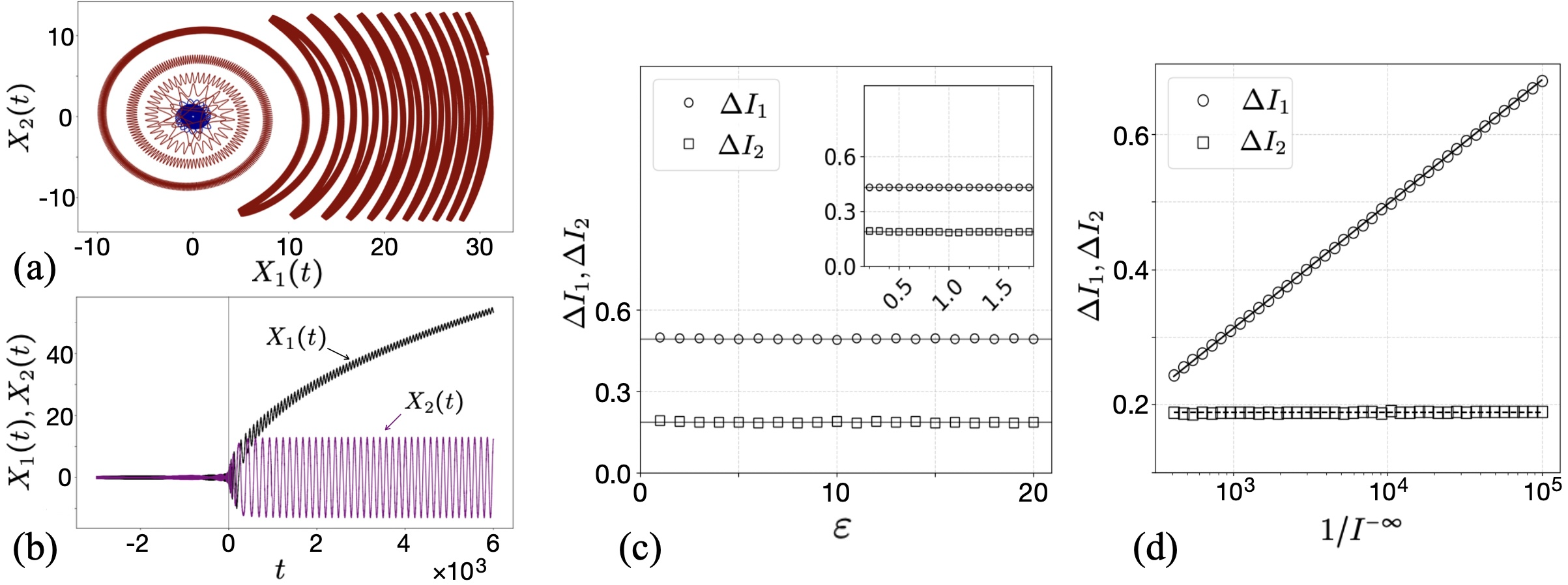
Figure 1: (a) Trajectory $\{X_{1}(t),X_{2}(t)\}$ for $t\in[-3000,2000]$ (blue: $t<0$, red: $t>0$) and the Hamiltonian (9); $\varepsilon=0.001$, $e_{1}=-1/2$, $e_{2}=1/2$, $X_{1}(t=-3000)=X_{2}(t=-3000)=-0.1$, $P_{1}(t=-3000)=-20$, $P_{2}(t=-3000)=20$. (b) Coordinates $X_{1}(t)$ (black) and $X_{2}(t)$ (purple) as functions of time for the same $\varepsilon$, $e_{1,2}$, and initial conditions. After the phase transition at $t=0$, both $X_{1}$ and $X_{2}$ pick up the amplitude with initially equal rate but for longer times, $t>1/\varepsilon$, $X_{1}(t)$ keeps growing, while $X_{2}(t)$ oscillates near $\langle X_{2}\rangle=0$. (c) Numerical check for $\varepsilon$-independent behaviour of $\Delta I_{1,2}$ at $I^{-\infty}_{1,2}=0.0001$. The inset resolves the interval $\varepsilon\in[0.2,1.8]$. The time interval for simulations is $t\in(-500,3000)$ and the time-step is $dt=0.0005$. Each point is the average of the final adiabatic invariant over $6000$ trajectories with different initial angles, in the action-angle variables, taken from a uniform distribution $\varphi_{1,2}\in(0,2\pi)$. (d) Numerical confirmation for Eq. (19): the logarithmic dependence of $\Delta I_{1}$ on $I_{1,2}^{-\infty}=I^{-\infty}$ and a constant value for $\Delta I_{2}$. Here, $\varepsilon=1$ and the other parameters are as in (c).

Our main result is that the saddle-point equations for the time-evolution with the potential energy (5) lead to a highly asymmetric final state no matter how small $\varepsilon$ is, as depicted in Fig. 1(a,b). Moreover, such equations are integrable, which allows us to characterize the nonadiabatic excitations analytically exactly. Thus, the model (1) has two excitation types over the minimum (3): the massless Goldstone and the massive Higgs bosons. One may expect that the nearly-massless Goldstone bosons are easier to produce but we will show that the Higgs bosons are produced in march larger quantities.

With a dynamic contribution to the effective action $S[{\bm{\pi}}(t){\bm{\phi}}(t)]$, the model acquires the form of the $0+1$-dimensional quantum field theory

$$S[{\bm{\pi}}(t){\bm{\phi}}(t)]=\int\left[\sum_{k=1,2}\pi_{k}\,d\phi_{k}-H({\bm{\pi}},{\bm{\phi}})\,dt\right],$$ (7)

where the Hamiltonian $H({\bm{\pi}},{\bm{\phi}})$ has a kinetic energy that depends on the momenta $\pi_{k}$ conjugate to $\phi_{k}$:

$$H({\bm{\pi}},{\bm{\phi}})=\sum_{k=1,2}\frac{\pi_{1}^{2}+\pi_{2}^{2}}{2m}+V({\bm{\phi}}),$$

and $m$ is an effective mass parameter. The saddle-point equations of motion are given by LL

$$\frac{d\phi_{k}}{dt}=\frac{\partial H}{\partial\pi_{k}},\quad\frac{d\pi_{k}}{dt}=-\frac{\partial H}{\partial\phi_{k}}.$$ (8)

Let us rescale variables by factors, $\lambda$, $u$ and $v$, so that

$$t\rightarrow\lambda t,\quad\pi_{k}=vP_{k},\quad\phi_{k}=uX_{k},\quad k=1,2.$$

In terms of $P_{k}$ and $X_{k}$, Eqs. (8) are still canonical with a new Hamiltonian ${\cal H}({\bf X},{\bf P})=\lambda H(u{\bf X},v{\bf P})/uv$, where ${\bf X}=(X_{1},X_{2})$ and ${\bf P}=(P_{1},P_{2})$. We choose the factors so that the symmetric terms of the Hamiltonian have only numerical coefficients:

$${\cal H}=\frac{{\bm{P}}^{2}}{2}-t\frac{{\bm{X}}^{2}}{2}+\frac{{\bm{X}}^{4}}{2}+\varepsilon\left(e_{1}X_{1}^{2}+e_{2}X_{2}^{2}\right),$$ (9)

which is achieved at $\lambda=(m/\beta)^{1/3},\,u=m^{1/6}\beta^{1/3}/\sqrt{g},\,v=m^{5/6}\beta^{2/3}/\sqrt{g}$, so that $e_{k}=\varepsilon_{k}\lambda u/v=\varepsilon_{k}/(\beta^{2}m)^{1/3}$.

As $t\rightarrow\pm\infty$, the evolution is adiabatic, and thus conserving the adiabatic invariants LL :

$$I_{k}=\frac{1}{\pi}\int_{x_{k}^{-}}^{x_{k}^{+}}dX_{k}\,P(X_{k}),\quad k=1,2,$$

where $x_{k}^{\pm}$ are the turning points of the classical trajectory (8). In quantum mechanics, this invariant is related to the number of excitations $n_{k}$ of the quantum fields $\phi_{k}$ over the ground level. Thus, in terms of the physical variables the adiabatic invariant is given by

$${\cal I}_{k}\equiv\frac{1}{\pi}\int_{\phi_{k}^{-}}^{\phi_{k}^{+}}\pi_{k}\,d\phi_{k}=\hbar(n_{k}+1/2).$$

We assume that the system is in the vacuum state as $t\rightarrow-\infty$, which corresponds to ${\cal I}_{1,2}^{-\infty}=\hbar/2$. The corresponding canonically conjugate angle variables $\varphi_{1,2}$ are not determined initially. The following, both analytical and numerical, results describe the averaging over uniformly distributed $\varphi_{1,2}\in[0,2\pi)$. Our change of variables was noncanonical, so

$${\cal I}_{k}^{\pm\infty}=I_{k}^{\pm\infty}uv=m\beta I_{k}^{\pm\infty}/g,$$ (10)

and the evolution with ${\cal H}$ starts with a small, $O(\hbar)$, value $I_{k}^{-\infty}=\hbar g/(2\beta m)\ll 1$.

To characterize the nonadiabatic effects we should find the asymptotic value of the average $\langle I_{k}\rangle$ over the initial conditions as $t\rightarrow+\infty$: $\langle I_{k}^{+\infty}\rangle=I_{k}^{ad}+\Delta I_{k}$, where $I_{k}^{ad}$ is the adiabatic invariant that would be found in the limit of the adiabatic evolution. The number of nonadaibatic excitations of $\phi_{k}$ is then given by

$$n_{k}=\beta m\Delta I_{k}/(\hbar g).$$ (11)

Our most nontrivial finding is that the function

$${\cal H}^{\prime}\equiv t(e_{1}X_{1}^{2}+e_{2}X_{2}^{2})-2\varepsilon(e_{1}^{2}X_{1}^{2}+e_{2}^{2}X_{2}^{2})-$$ (12)

$$e_{1}(P_{1}^{2}+X_{1}^{4}+X_{1}^{2}X_{2}^{2})-e_{2}(P_{2}^{2}+X_{1}^{2}X_{2}^{2}+X_{2}^{4})+\frac{L^{2}}{2\varepsilon},$$

where $L=P_{2}X_{1}-P_{1}X_{2}$ is the angular momentum, satisfies the following relations with ${\cal H}$, from Eq (9):

$$\frac{\partial{\cal H}}{\partial\varepsilon} = \frac{\partial H^{\prime}}{\partial t},$$

$$\{{\cal H},{\cal H}^{\prime}\} \equiv \sum_{k=1,2}\frac{\partial{\cal H}}{\partial X_{k}}\frac{\partial{\cal H^{\prime}}}{\partial P_{k}}-\frac{\partial{\cal H}}{\partial P_{k}}\frac{\partial{\cal H^{\prime}}}{\partial X_{k}}=0.$$ (13)

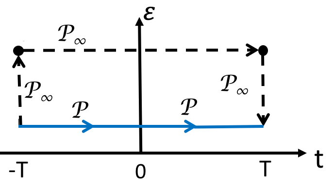
Figure 2: The physical path, ${\cal P}$, of the evolution in $(t,\varepsilon)$ plane goes through a critical point at $t\approx 0$ at fixed $\varepsilon\ll\beta/g$. Here, $T\rightarrow\infty$. The path ${\cal P}_{\infty}$ initially lifts $\varepsilon$ with the Hamiltonian ${\cal H^{\prime}}$ to a large value $\varepsilon\gg\beta/g$ at formally infinite $|t|$. The horizontal part of ${\cal P}_{\infty}$ produces the evolution with ${\cal H}$ at large rather than small fixed $\varepsilon$. The second vertical leg of ${\cal P}_{\infty}$ brings the system back to small $\varepsilon$ at infinite $t$.

This makes the 1-form

$$\Omega={\cal H}\,dt+{\cal H}^{\prime}\,d\varepsilon$$

closed. In appendix A, we show that the integration of the classical equations of motion can then be extended to a two-time $\tau$-plane $(\tau_{1},\tau_{2})\equiv(t,\varepsilon)$ with a two-Hamiltonian $({\cal H}_{1},{\cal H}_{2})=({\cal H},{\cal H^{\prime}})$, so that

$$\frac{\partial X_{k}}{\partial\tau_{j}}=\frac{\partial{\cal H}_{j}}{\partial P_{k}},\quad\frac{\partial P_{k}}{\partial\tau_{j}}=-\frac{\partial{\cal H}_{j}}{\partial X_{k}},\quad k,j=1,2.$$

Analogously to the integrable multistate Landau-Zener models commute ; parallel , the result of the evolution along an arbitrary path in the $\tau$-plane then depends only on the initial and final two-time-points but does not depend on the choice of the path that connects them, as long as this path does not cross the singular point of ${\cal H}^{\prime}$ at $\varepsilon=0$. Our original physical evolution corresponds to the path ${\cal P}$, shown in Fig. 2. To avoid any complex dynamics encountered along ${\cal P}$ near $t=0$, we deform it into the path ${\cal P}_{\infty}$ that bypasses this region from a large distance.

Along the left vertical leg of ${\cal P}_{\infty}$, the dynamics is dominated by the $t$-dependent terms because $t\rightarrow-\infty$. Keeping only the most relevant terms we find for this piece

$$d^{2}X_{k}/d^{2}\varepsilon+(2e_{k})^{2}|t|X_{k}=0,\quad k=1,2,$$

which corresponds to the harmonic oscillators with formally infinite frequencies.

Thus, the first vertical leg produces only the adiabatic dynamics that conserves $I_{1,2}$. It merely brings the system to the point with large $\varepsilon$, such that $\varepsilon e_{k}\gg\beta/g$. Analogously, along the other vertical part of ${\cal P}_{\infty}$, the nonadiabatic transitions are suppressed by a formally infinite value of $t$.

The evolution along the horizontal part of ${\cal P}_{\infty}$ proceeds during $t\in(-\infty,\infty)$ with the Hamiltonian ${\cal H}$ at very large $\varepsilon$. The main consequence of the model’s integrability is then the independence of the evolution result, for the Hamiltonian (9), of the strength of the symmetry breaking parameter $\varepsilon$, $\varepsilon>0$, which we verified numerically in Fig. 1(c). Hence, it is sufficient for our goals to study the case of $\varepsilon\gg g,\beta^{1/2}$ to describe arbitrary symmetry breaking.

At large $\varepsilon$, $X_{1}$ enters the phase transition at $t_{1}=2\varepsilon e_{1}$, which is now long before the critical moment for $X_{2}$, at $t_{2}=2\varepsilon e_{2}$. Near $t=t_{1}$, the variable $X_{2}$ experiences a strong confinement in the quadratic potential $\sim\varepsilon(\varepsilon_{2}-\varepsilon_{1})X_{2}^{2}$, and for large $\varepsilon$ performs fast oscillations, whose effect on $X_{1}$ averages to zero. The evolution of $X_{1}$ is then governed by the truncated to $(X_{1},P_{1})$ Hamiltonian ${\cal H}_{1}=P_{1}^{2}/2-sX_{1}^{2}/2+X_{1}^{4}/2$, where $s=t-2\varepsilon e_{1}$. The corresponding equation of motion

$$d^{2}X_{1}/ds^{2}=sX_{1}-2X_{1}^{3}$$ (14)

is the Painleve-2 equation, whose solution has known asymptotic behavior P2-book as $s\rightarrow+\infty$:

$$\begin{split}X_{1}(s)&=\pm\sqrt{\frac{s}{2}}\\ &\pm\rho(2s)^{-1/4}\cos\left(\frac{2\sqrt{2}}{3}s^{3/2}-\frac{3}{2}\rho^{2}\ln s+\theta(\varphi_{0})\right),\end{split}$$ (15)

where $\rho=\sqrt{2I^{+\infty}}$, and the term $\pm\sqrt{s/2}$ corresponds to the time-dependent positions of the new potential minima. In appendix B, we derive the change of the adiabatic invariant for Eq. (14) for small initial $I_{1}^{-\infty}$:

$$\Delta I_{1}=I_{1}^{+\infty}-I_{1}^{-\infty}/2=\frac{1}{4\pi}\ln\left(\frac{1}{2\pi I_{1}^{-\infty}}\right).$$ (16)

After the transition through the first critical point, at $t=2\varepsilon e_{1}$, along the horizontal leg of ${\cal P}_{\infty}$, the variable $X_{1}$ is dominated by the growing contribution $X_{1}^{2}\sim s/2=(t-2\varepsilon e_{2})/2$. Substituting this into the Hamiltonian ${\cal H}$, we find the effective Hamiltonian for $X_{2}$:

$${\cal H}_{2}=\frac{P_{2}^{2}}{2}+\varepsilon(e_{2}-e_{1})X_{2}^{2}+X_{2}^{4}/2.$$

Importantly, this Hamiltonian does not depend on $t$ explicitly. Since $e_{2}>e_{1}$, small excitations are confined by a nearly-harmonic potential with the frequency

$$\omega_{2}=\sqrt{2\varepsilon(e_{2}-e_{1})}.$$ (17)

In the rest of ${\cal P}_{\infty}$ the evolution for $X_{2}$ does not go through a new critical point. As $t\rightarrow+\infty$, the variable $X_{2}$ oscillates near the local minimum.

Thus, the variable $X_{2}$ is not growing permanently with time and hence the field $\phi_{2}$ at the end of the evolution does not form a condensate. No matter how small the physical parameter $\varepsilon$ can be in comparison to the interaction and dynamic parameters, the macroscopic condensate is always created only by the field $\phi_{1}$.

The nonadiabatic excitations for $X_{2}$, are smaller but finite. They follow from the fact that, after the symmetry breaking for $X_{1}$, the frequency of the oscillatory component of $X_{1}$ in (15) grows as $\omega_{1}\approx\sqrt{2(t-\varepsilon e_{1})}$. Hence, at the distant from $t_{1}$ moment, $t_{2}=\varepsilon e_{2}$, the nonadiabatic excitations for $X_{1}$ and $X_{2}$ enter in a resonance, and can exchange their power due to the nonlinear interaction terms. We found numerically (Fig. 1(d)) that for small initial $I_{2}^{-\infty}=I_{1}^{-\infty}$, this resonance produces only subdominant excitations that appear as a non-logarithmic correction, so that

$$\Delta I_{1}=\frac{1}{4\pi}\left[\ln\left(\frac{1}{2\pi I_{1}^{-\infty}}\right)-c_{1}\right],\quad\Delta I_{2}=\frac{c_{2}}{2\pi},$$ (18)

where we determined that $c_{1}=1.14$ and $c_{2}=1.19$ are constants that do not depend on the initial conditions as long as $I_{1}^{-\infty}=I_{2}^{-\infty}\ll 1$. By restoring the physical variables via (10) and (11), we find the excitation numbers

$$n_{1}=\frac{\beta m}{4\pi g\hbar}\left[\ln\left(\frac{\beta m}{\pi\hbar g}\right)-c_{1}\right],\quad n_{2}=\frac{c_{2}\beta m}{2\pi g\hbar}.$$ (19)

Since $\phi_{1}$ forms the condensate, its oscillatory excitations are the Higgs bosons. Their average number is given by $n_{1}$ in (19). The excitations of the field $\phi_{2}$ are massless in the limit $\varepsilon\rightarrow 0$, so they are the Goldstone bosons.

For specific applications, the parameters $m$ and $g$ are to be determined by further details of the models, beyond the effective field theory, and the constants $c_{1,2}$ can be affected by the quantum corrections to our assumption that initially ${\cal I}_{1,2}^{-\infty}=\hbar/2$. However, the scaling, $n_{1}\sim\Gamma\ln\Gamma$ and $n_{2}\sim\Gamma\equiv\beta m/(g\hbar)$, is our prediction for the Kibble-Zurek exponent of the universality class described by the mean field theory (9).

Our results give rise to speculations about the origin of the matter-antimatter asymmetry, given the smallness of the CP-violation in the Standard Model. We have shown that the cosmological waterfall-like models can explain a strong asymmetry in particle production. Our scaling predictions should also be verifiable with experiments on reactions between ultracold atoms and molecular condensates, which leads to the second order quantum phase transition when a magnetic field sweeps the atoms in an optical trap through the Feshbach resonance itin . This may also have applications for the problem of separation of isotopes with similar masses by driving their mixture through a critical point sinitsyn-21prl .

Finally, our approach shows that the integrability of the Painleve equations can be generalized to multi-dimensional Hamiltonian equations, with possibility to connect asymptotic solutions as $t\rightarrow\pm\infty$. Our model (9) can be generalized to a multi-dimensional system with

$${\cal H}=\sum_{k=1}^{N}\left[\frac{P_{k}^{2}}{2}-t\frac{X_{k}^{2}}{2}+\varepsilon e_{k}X_{k}^{2}\right]+\frac{\left(\sum_{k=1}^{N}X_{k}^{2}\right)^{2}}{2},$$ (20)

where $N$ is an arbitrary integer number of degrees of freedom, $t$ is time and $e_{1}<e_{2}<\ldots<e_{N}$ are arbitrary parameters. Another Hamiltonian

$${\cal H}^{\prime}\!\equiv\!\sum_{k=1}^{N}\left[-2\varepsilon e_{k}^{2}X_{k}^{2}+e_{k}(tX_{k}^{2}\!-\!P_{k}^{2}-X_{k}^{2}\sum_{j=1}^{N}X_{k}^{2}X_{j}^{2})\right]\!+\!\frac{{\bf L}^{2}}{2\varepsilon},$$

where ${\bf L}$ is the vector of total angular momentum, satisfies the integrability conditions with ${\cal H}$: $\{{\cal H},{\cal H}^{\prime}\}=0$ and $\partial_{\varepsilon}{\cal H}=\partial_{t}{\cal H}^{\prime}$. It should be insightful in the future to find other integrable nontrivial pairs of Hamiltonians that depend only linearly or inversely linearly on $t$ and $\varepsilon$. This should also advance our understanding of the purely dynamic nonperturbative effects in critical phenomena.

Appendix A Integrability conditions

Here, we review the notion of an integrable family of classical Hamiltonians. Let $X$ be a phase space, i.e., a smooth manifold, equipped with a Poisson bracket

$$\{f,g\}=\sum_{ij}\omega_{ij}(x)\frac{\partial f}{\partial x_{i}}\frac{\partial g}{\partial x_{j}},$$ (21)

with $f,g\in{\cal H}$, with ${\cal H}$ being the vector space of smooth functions on $X$, and let $\{H_{\alpha}(\bm{\tau})\,|\,\alpha=1,\ldots,n,\,|\,\bm{\tau}\in U\}$ be a smooth family of classical Hamiltonians over an open single connected region $U\subset\mathbb{R}^{n}$. Then any smooth path $\bm{\tau}:[0,1]\to U$ defines a time-dependent Hamiltonian $H(t)=\sum_{\alpha}\dot{\tau}_{\alpha}H_{\alpha}(\bm{\tau}(t))$. Our goal is to identify the explicit conditions for integrability, i.e., that the solution of the Hamilton equation

$$\dot{x}_{j}=\sum_{k}\omega_{jk}(x(t))\frac{\partial H(\bm{\tau}(t),x)}{\partial x_{k}},$$ (22)

depends on the initial condition, as well as the initial and final points of a path $\tau$, and is independent of a particular choice of a path. Since the Hamilton equation is equivalent to the Liouville equation

$$\dot{f}=\{H(\bm{\tau}(t)),f\}$$ (23)

for the evolutions of functions/distributions $f\in{\cal H}$, the inegrability conditions can be alternatively identified for Eq. (23), rather than (22). Indeed, the Poisson bracket equip ${\cal H}$ with a structure of an infinite-dimensional Lia algebra, and

$$\nabla_{\alpha}f=\frac{\partial f}{\partial\tau_{\alpha}}-\{H_{\alpha},f\},$$ (24)

define a non-abelian connection/gauge field/covariant derivative in a trivial infinite-dimensional vector bundle ${\cal H}\times U\to U$ with the fiber ${\cal H}$ and structure/gauge group $G$ being the group of canonical diffeomorphisms/transformations of $X$. According to commute , the integribility conditions are given by vanishing of the curvature ${\cal F}$ of the connection, defined in Eq. (24):

$${\cal F}_{\alpha\beta}=\frac{\partial H_{\alpha}}{\partial\tau_{\beta}}-\frac{\partial H_{\beta}}{\partial\tau_{\alpha}}-\{H_{\alpha},H_{\beta}\}=0.$$ (25)

Appendix B Asymptotic solution of Painleve-2

We will follow closely the analysis in itin , which is based on the known asymptotic solutions of the Painleve-2 P2-book . Starting as $s\rightarrow-\infty$ the Painleve-2 equation describes trivial oscillations in a harmonic potential:

$$X_{1}(s)=\alpha(-s)^{-1/4}\sin\left(\frac{2}{3}(-s)^{3/2}+\frac{3}{4}\alpha^{2}\ln(-s)+\varphi_{0}\right),$$

For $s\rightarrow+\infty$:

$$\begin{split}&X_{1}(s)=\pm\sqrt{\frac{s}{2}}\\ &\pm\rho(2s)^{-1/4}\cos\left(\frac{2\sqrt{2}}{3}s^{3/2}-\frac{3}{2}\rho^{2}\ln s+\theta(\varphi_{0})\right),\end{split}$$ (26)

where the term $\pm\sqrt{s/2}$ corresponds to the time-dependent positions of the new potential minima, and

$$\rho^{2}=\frac{1}{\pi}\ln\frac{1+|p|^{2}}{2|\Im(p)|},\quad p=\sqrt{e^{\pi\alpha^{2}}-1}e^{i\theta^{\prime}(\varphi_{0})},$$ (27)

where $\theta$, $\theta^{\prime}$ are phases whose precise values are not needed for our discussion because we should average the final result over the initial phase $\varphi_{0}$, and hence over $\theta$ and $\theta^{\prime}$.

The oscillatory terms in $X_{1}$ are due to the excitations. Long before the critical point the system is in a parabolic potential with frequency $\omega_{-\infty}=\sqrt{|s|}$, and long after the critical point, $\omega_{+\infty}=\sqrt{2s}$. For the harmonic oscillator, the half-axis of the oscillation and the adiabatic invariant, $I_{1}$, are related by $I_{1}=\Delta X_{1}^{2}\omega/2$ LL , so we can now identify

$$I_{1}^{-{\infty}}=\alpha^{2}/2,\quad I_{1}^{+\infty}=\rho^{2}/2.$$ (28)

The nonadiabatic shift of this invariant is given by $\Delta I_{1}=I_{1}^{+\infty}-I_{1}^{-\infty}/2$, where $1/2$ is a purely geometric effect that reflects the change of the phase space volume by a trajectory at crossing the separatrix of the double well potential. We then write $p=|p|e^{i\pi\xi}$, where $\xi$ is treated as a uniformly random number $\xi\in(0,1)$. Substituting this into Eqs. (26)-(27), and averaging over $\xi$, we find

$$\Delta I_{1}=-\frac{1}{4\pi}\ln\left(1-e^{-2\pi I_{1}^{-{\infty}}}\right).$$ (29)

For $I_{1}^{-\infty}\ll 1$, we arrive at Eq. (16) in the main text.

References

(1)
Andrei Linde.
Phys. Rev. D 49, 748 (1994). Hybrid inflation.
(2)
L. Kofman, A. Linde, and A. A. Starobinsky.
Phys. Rev. Lett. 73, 3195 (1994). Reheating after Inflation.
(3)
E. J. Copeland, S. Pascoli, and A. Rajantie.
Phys. Rev. D 65, 103517 (2002) Dynamics of tachyonic preheating after hybrid inflation.
(4) A. Altland, V. Gurarie, T. Kriecherbauer, and A. Polkovnikov.
Phys. Rev. A 79, 042703 (2009). Nonadiabaticity and large fluctuations in a many-particle Landau-Zener problem.
(5) A.P. Itin, P. Törmä. Preprint arXiv:0901.4778 (2009) Dynamics of quantum phase transitions in Dicke and Lipkin-Meshkov-Glick models.; V. Ganesh Sadhasivam, F. Suzuki, B. Yan, N. A. Sinitsyn. Preprint arXiv:2403.09291 (2024). Parametric tuning of dynamical phase transitions in ultracold reactions.
(6) T. W. B. Kibble J. Phys. A: Math. Gen. 9 1387 (1976). Topology of cosmic domains and strings.
(7) V. M. G. Silveira, C. A. Z. Vasconcellos, E. G. S. Luna, D. Hadjimichef.
J. High Energy Phys. 2021 285 (2021). Matter-antimatter asymmetry and non-inertial effects.
(8) L. D. Landau and E. M. Lifshitz. Vol. I, Nauka, Moskva (1973). Classicheskaya Mehanika. (in Russian).
(9) N. A. Sinitsyn, E. A. Yuzbashyan, V. Y. Chernyak, A. Patra, and C. Sun. Phys. Rev. Lett. 120, 190402 (2018). Integrable time-dependent quantum Hamiltonians.
(10) V. Y. Chernyak, F. Li, C. Sun, and N. A. Sinitsyn. J. Phys. A: Math. Theor. 51 245201 (2020). Integrable multistate Landau-Zener models with parallel energy levels.
(11)
A. S. Fokas, A. R. Its, A. A. Kapaev, V. Yu. Novokshenov. Painleve Transcendents: The Riemann-Hilbert Approach. Mathematical Surveys and Monographs (Mathematical Surveys and Monographs, 128), American Mathematical Society (October 10, 2006).
(12)
B. Yan, V. Y. Chernyak, W. H. Zurek, and N. A. Sinitsyn.
Phys. Rev. Lett. 126, 070602 (2021). Nonadiabatic Phase Transition with Broken Chiral Symmetry.