The ESO UVES/FEROS Large Programs of TESS OB pulsators

Abstract

Context. Spectral lines of hot massive stars are known to exhibit large excess broadening in addition to rotational broadening. This excess broadening is often attributed to macroturbulence whose physical origin is a matter of active debate in the stellar astrophysics community.

Aims. We aim to shed light on the physical origin of macroturbulent line broadening by looking into the statistical properties of a large sample of O- and B-type stars, both in the Galaxy and LMC.

Methods. We deliver newly measured macroturbulent velocities for 86 stars from the Galaxy in a consistent manner with 126 stars from the LMC. A total sample of 594 stars with measured macroturbulent velocities was composed by complementing our sample with archival data for the Galactic O- and B-type stars for a better coverage of the parameter space. Furthermore, we compute an extensive grid of mesa models to compare, in a statistical manner, the predicted interior properties of stars (such as convection and wave propagation) with the inferrence of macroturbulent velocities from high-resolution spectroscopic observations.

Results. We find evidence for subsurface convective zones formed in the iron opacity bump (FeCZ) being connected to observed macroturbulent velocities in hot massive stars. Additionally, we find the presence of two principally different regimes where, depending on the initial stellar mass, different mechanisms may be responsible for the observed excess line broadening.

Conclusions. Stars with initial masses above some 30$M_{\odot}$ have macroturbulent velocities fully determined by FeCZ, while some other mechanism is required to explain observations for masses below 12$M_{\odot}$. The latter finding leaves the potential for waves generated at the interface of the convective core and radiative envelope of the star to be responsible for the observed macroturbulent broadening. Both mechanisms may co-exist in the intermediate regime of stellar masses, between some 12 and 30$M_{\odot}$.

1 Introduction

Macroturbulent line broadening in stellar spectra refers to the broadening of spectral lines caused by large-scale turbulent motions in the stellar atmospheres. Historically, macroturbulent line broadening was identified as a key mechanism decades ago, when it was noticed that rotational broadening alone could not account for the observed widths and shapes of spectral lines. This led to the development of models incorporating large-scale atmospheric turbulence. A comprehensive review on the matter exists thanks to Gray (1978, 2008), or, concerning massive stars, Howarth (2004).

Particularly strong macroturbulent broadening was found in spectral lines of massive stars, characterised by macroturbulent velocities $\Theta$ ten times larger than those found in solar-type stars, often dominating over thte rotational broadening. The need for excessive broadening in massive stars was quantified by Howarth et al. (1997). The authors measured total broadening in 373 O- and B- type supergiants in a self-consistent way by cross-correlating all observed spectra with one observed template spectrum. They reported the need for additional broadening mechanisms on top of the rotation to be able explain the observed total line broadening of over 100 km s^-1  for such a large sample, with presumably randomly distributed inclination angles.

With the development of models for macroturbulent line profiles, it became possible to fit the total shapes of individual line profiles by convolution of intrinsic line profiles with both rotational and macroturbulent profiles. Ryans et al. (2002) analysed high-resolution spectra of 12 B-type supergiants and found that rotational broadening alone was not sufficient to describe observed line profile shapes, and extra macroturbulent broadening of 20-60 km s^-1  had to be applied. Even higher macroturbulent velocities of up to 100 km s^-1  were found by Simón-Díaz et al. (2010) in a sample of 15 supergiants of late-O to B spectral types. The same results were later reported in larger samples, such as the sample of 430 O- and B- type Galactic stars analysed by Simón-Díaz et al. (2017) and the sample of 126 B-type supergiants from the LMC analysed by Serebriakova et al. (2023).

The physical origin of such large velocities present in the photospheres of hot massive stars is still debated. In the Sun, photospheric granulation is directly observed and leads to the macroturbulent broadening of lines in the solar spectrum (and spectra of other solar-type stars). Massive hot stars have radiative envelopes, hence, the macroturbulent broadening in these stars requires another physical explanation. Often it is attributed to the excitation of multiple non-radial pulsations modes (Lucy (1976); Kaufer et al. (1997); Ryans et al. (2002); Howarth (2004)). Kaufer et al. (1997) performed a long-term monitoring of 6 BA supergiants and reported variability in radial velocities and line strengths with multiple-mode cyclic behaviour on time scales of 5 to 50 days. The authors attributed the detected variability to the effect of non-radial oscillations on the stellar surface. Aerts et al. (2009a, b) modelled spectral line profiles by the collective effect of hundreds of low-amplitude non-radial gravity modes on top of rotation. The authors reported that the resulting macroturbulent profile mimics these collective pulsational effects, and ignoring time-dependent waves leads to single snapshot line profiles with global velocity fields of unrealistic (sometimes supersonic) scale.

While there seems to be agreement that macroturbulent velocities originate from pulsation modes and internal gravity waves (IGW), the debates are focused on where they get excited: at the interface of the convective core and the radiative envelope (Rogers et al. (2013)) or subsurface convective layers. The subsurface convective layers originate in radiative envelopes of massive stars with an initial mass larger than some 10 $M_{\odot}$ due to the iron (FeCZ) or helium (HeCZ) opacity bumps. Cantiello et al. (2009) computed models of interiors of stars with masses from 5 to 100 $M_{\odot}$ and found correlations between the presence of FeCZ and observed microturbulent velocities $\xi$ and wind clumping. Furthermore, Grassitelli et al. (2015, 2016) investigated FeCZ and found that areas of high turbulent pressure in these subsurface convective layers, when mapped to the positions in Hertzsprung-Russell diagram (HRD), aligned nicely with regions where observations showed an excess of stars with high macroturbulent velocity values. This result was reinforced by the conclusions of Simón-Díaz et al. (2017) who analysed macroturbulent velocities in a large sample of 430 massive stars.

The debates were boosted with the discovery of stochastic low-frequency variability (SLFV) in space photometry of O- and B-type stars. The SLFV manifests itself as a power excess in the low-frequency part of the Fourier spectrum. While the first observational detections of SLFV date back to CoRoT and early $Kepler$ times (e.g., Blomme et al., 2011; Tkachenko et al., 2014; Aerts et al., 2017), detailed observational studies and interpretation were first presented in Bowman et al. (2019a, b). Furthermore, Burssens et al. (2020) and Bowman et al. (2020) found a correlation between SLFV properties and macroturbulent broadening, a finding suggestive of a connection between the two observed phenomena, both caused by the modes excited near the boundary of the convective core.

Lecoanet et al. (2019, 2021) provided a theoretical model for internal gravity waves (IGWs) and concluded that the calculated surface manifestation does not correlate with the observed SLFV nor macroturbulence. At the same time, Edelmann et al. (2019) and Vanon et al. (2023) performed 3D simulations of core convection for 3 and 7$M_{\odot}$ stellar models, respectively, and reported theoretical frequency spectra to have properties similar to those of the observed SLFV. In particular, the authors noted a pronounced low-frequency excess present in the models with the frequency range decreasing with stellar age. Furthermore, Ratnasingam et al. (2020) and Ratnasingam et al. (2023) performed 2D simulations and computed frequency spectra of IGWs from 3, 5, 7, 10, and 13$M_{\odot}$ stellar models. The authors reported the slopes of the frequency spectra to be in agreement with observed properties of SLFV. Anders et al. (2023) challenged higher masses and performed comprehensive simulations of core convection for 3, 15 and 40$M_{\odot}$ stellar models at the zero age main sequence (ZAMS). From their simulations, the authors predicted the frequency spectra of the gravity waves propagated to the surface. Contrary to the previous findings based on 2- and 3-D simulations, Anders et al. (2023) concluded that all three models predict variability amplitudes several orders of magnitude lower than both observed SLFV amplitudes and current observational detection capabilities.

Apart from IGWs, the subsurface convective layers were also simulated and tested as a plausible explanation of SLFV and macroturbulent broadening. Cantiello et al. (2021) found that model properties of FeCZ from 1D mesa simulations in a large range of masses and ages correlate well with both SLFV and macroturbulence. A similar conclusion was presented in Ma et al. (2024). 3D simulations of exteriors were computed by Schultz et al. (2022) and Schultz et al. (2023a) for a 13$M_{\odot}$ star at terminal age main sequence (TAMS), 35$M_{\odot}$ star at ZAMS and at mid-main sequence, and 56 and 80$M_{\odot}$ stars in the Hertzsprung gap. The authors concluded that FeCZ and HeCZ extend significantly further in radial direction compared to 1D models and reach stellar photosphere. The resulting large turbulent velocities at the stellar surface were found in agreement with similarly large observed macroturbulent velocities. Moreover, the same models were used by Schultz et al. (2023b) to synthesise spectral line profiles broadened by the clumpy turbulent surface. The authors concluded on the similarity between the shapes of the macroturbulent broadening-dominated profile and their simulated line profiles.

In this study, we present a statistical analysis of sample of 594 stars for which observational inference of the macroturbulent velocity is avalible. The sample covers masses from 2.5 to 80 $M_{\odot}$ and two metallicity regimes (LMC and the Galaxy). For 86 stars, we present macroturbulent velocities measured for the first time. In addition to the observed sample, we compute a dense grid of mesa stellar structure and evolution models and investigate the properties of FeCZ and HeCZ across the HRD. We compare statistical properties of the observed sample and model properties of FeCZ in order to examine their possible connection. Moreover, for the full grid of models, we estimate the theoretical possibility of IGWs tunnelling through convective layers and assess its possible connection to the observations.

The full description of observations and analyses involved in the sample is given in section 2. Section 3 summarises input physics included in the computation of the mesa models. Section 4 is dedicated to qualitative and quantitative analyses of the observed macroturbulent velocities and model convective velocities, delving into multivariate linear regression in subsection 4.1 and principal component analysis in subsection 4.2. Finally, section 5 explores IGWs propagation properties. The conclusions of our study are presented in section 6.

2 Observed sample, data reduction, and spectroscopic parameter determination

Our study focuses on a comprehensive sample of stars covering a mass range from 2.5 to 80 $M_{\odot}$ with measured macroturbulent velocities $\Theta$. The sample consists of data from two ESO Large Programs using the uves and feros spectrographs: 126 supergiants (SG) in the Large Magellanic Cloud (LMC) from Serebriakova et al. (2023), 86 Galactic main-sequence (MS) stars from Gebruers et al. (2022), and 382 Galactic MS and SG stars from Simón-Díaz et al. (2017). This results in a total of 594 stars, covering metallicity regimes of the Milky Way (Solar metallicity of $Z$=0.014 is adopted for this regime) and LMC ($Z$=0.006) galaxies. The full sample is shown on the HRD in Fig.1. Note that hereafter we use spectroscopic luminosity $\mathcal{L}=\frac{T_{eff}^{4}}{g}$ following Simón-Díaz et al. (2017) in all plots since spectroscopic luminosity can be inferred directly from the observed $T_{\rm eff}$ and $\log g$ values without requiring to known the distance. At the same time, spectroscopic luminosity behaves similarly to the usual luminosity of the star (Langer & Kudritzki (2014)).

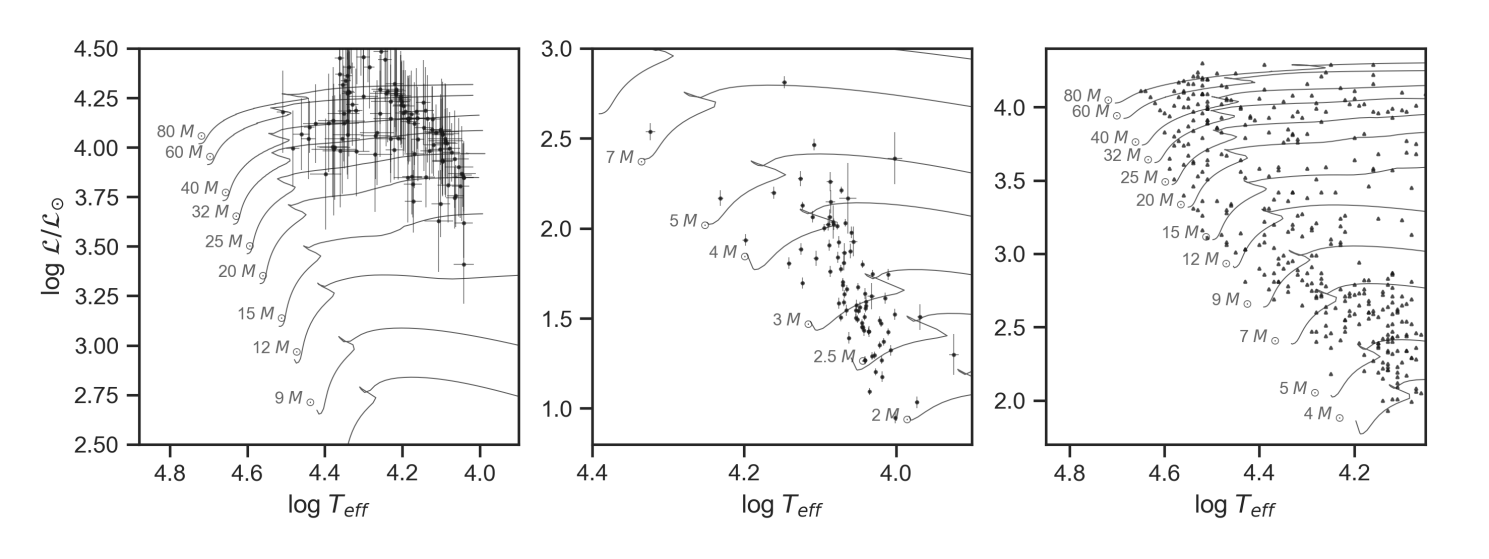
Figure 1: Full observed sample of high-mass stars with measured macroturbulent velocities. Left panel: LMC supergiants from Serebriakova et al. (2023) over evolutionary tracks for $Z$=0.006. Middle and right panels: Galactic objects from Gebruers et al. (2022) and Simón-Díaz et al. (2017), respectively, over evolutionary tracks for $Z$=0.014.

The data reduction, atmospheric parameter determination, and line broadening measurement for the three subsamples were handled primarily within their respective studies. Our work involved using the processed data and applying additional steps where necessary, specifically for the Galactic MS stars from Gebruers et al. (2022) where macroturbulent velocity measurements were not included in the analysis. The data reduction and processing varied slightly across the different subsamples due to the distinct methodologies employed in each of the referenced studies. Here, we provide a brief summary of the analyses employed for each subsample.

2.1 Subsample of LMC supergiants from Serebriakova et al. (2023)

The observations were conducted as part of the large programs using the uves instrument mounted on UT2 at the VLT (Dekker et al., 2000) and the feros instrument mounted on the MPG/ESO 2.2-m telescope (Kaufer et al., 1999). These programs aimed to deliver high-resolution, high signal-to-noise ratio spectroscopy of a sample of apparently single OB stars in the LMC. Each target was observed at two epochs separated by at least 2-3 weeks to detect potential spectral variability.

The data reduction process employed the EsoReflex data reduction pipeline for the uves spectra and the ceres (Brahm et al., 2017) pipeline for the feros spectra. Custom order-by-order normalisation was applied to correct for artefacts resulting from the order merging of the original pipelines.

The atmospheric parameters were determined using a grid search method involving the tlusty (Hubeny, 1988), cmfgen (Hillier & Lanz, 2001), and gssp (Tkachenko, 2015) model spectra, depending on the parameter range.

The projected rotational velocities $v\sin i$  were inferred using the Fourier transform (FT) method. This technique identifies the position of the first zero in the FT of a rotationally broadened profile, directly translating to the $v\sin i$  of the star. Specific spectral lines such as Si ii, Si iii, Mg ii, and He i were selected based on their suitability for different types of stars in the sample.

Macroturbulent velocities $\Theta$ were deduced by fitting synthetic spectra to observed line profiles of the Mg ii 4481 Å line. The synthetic intrinsic profiles in the form of specific intensities $I(\mu)$ were computed for every object’s given atmospheric parameters and convolved with a radial-tangential macroturbulent kernel. With the integration of $I(\mu)$ over the sphere, rotational broadening naturally included realistic limb darkening for the exact atmosphere model of each object. The projected rotational velocities were allowed to vary within 1$\sigma$ uncertainties of the values inferred with the FT method.

2.2 Subsample of Galactic main-sequence stars from Gebruers et al. (2022)

The observations were conducted as part of the same feros large program as in Serebriakova et al. (2023) albeit focused on Galactic main-sequence OB-type stars.

The modified ceres pipeline was employed for the extraction of stellar spectra. In the original study, the normalisation function was optimised together with atmospheric parameters. For the sake of consistency with Serebriakova et al. (2023), we employed the same order-by-order approach to normalise the spectra.

Atmospheric parameters were derived using the zeta-Payne (Straumit et al., 2022) pipeline, which employs a pre-trained neural network to predict normalised synthetic spectra for a given set of stellar labels ($T_{\rm eff}$, $\log g$, $v\sin i$, [M/H]). The normalisation function was optimised along with these labels.

Since $v\sin i$  derived by zeta-Payne represents the total broadening due to the collective effect of rotation and macroturbulence (as the latter was not included in the fitting), we additionally employed the same method as in Serebriakova et al. (2023) to infer $v\sin i$  values, namely, using the FT method to separate the rotational broadening.

The original study did not include measurements of $\Theta$, hence we repeated the same procedure as in Serebriakova et al. (2023) to infer $\Theta$, which implied fitting theMg ii 4481 Å line profile with both rotationally and macroturbulent broadened synthetic intrinsic profiles.

2.3 Subsample of Galactic main-sequence and supergiant stars from Simón-Díaz et al. (2017)

The sample was observed as part of the iacob project (Simón-Díaz et al., 2011), utilising high-resolution spectra from the fies (Telting et al., 2014) and hermes (Raskin et al., 2011) spectrographs attached to the 2.56-m Nordic Optical Telescope and 1.2-m Mercator Telescope, respectively.

The spectra were reduced using the FIEStool and HermesDRS pipelines for fies and hermes, respectively, followed by normalisation using custom procedures implemented in IDL.

The atmospheric parameters were obtained using the iacob-gbat tool with a grid of fastwind (Puls et al. (2005)) synthetic spectra.

Projected rotational velocities were determined using the iacob-broad tool, which combines the FT and goodness-of-fit (GOF) methodologies.

The same iacob-broad tool was used to fit radial-tangential macroturbulent and rotational profiles. The FT method provided initial estimates, while the GOF method was used to refine the final values for both broadenings.

2.4 A look into the full combined sample of the observed macroturbulent velocities $\Theta$

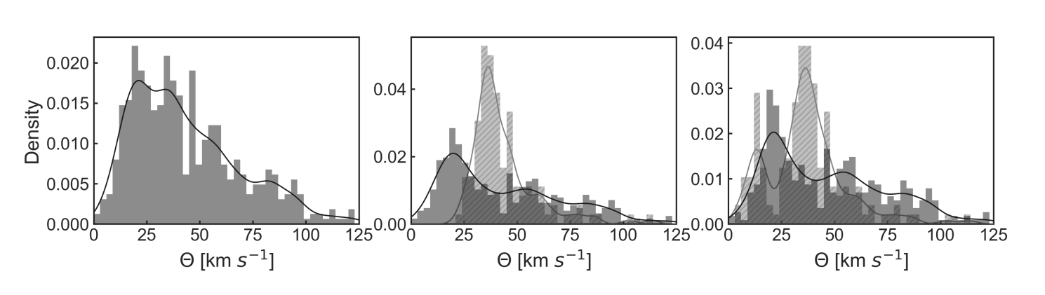
Figure 2: Histograms and Kernel Density Estimates (KDE, solid line) of the measured $\Theta$. From left to right: the full sample of 594 stars, Galactic (dark grey) versus LMC (light grey) stars, and stars for which macroturbulent velocities were inferred with the methods of Serebriakova et al. (2023, light grey) and Simón-Díaz et al. (2017, dark grey).

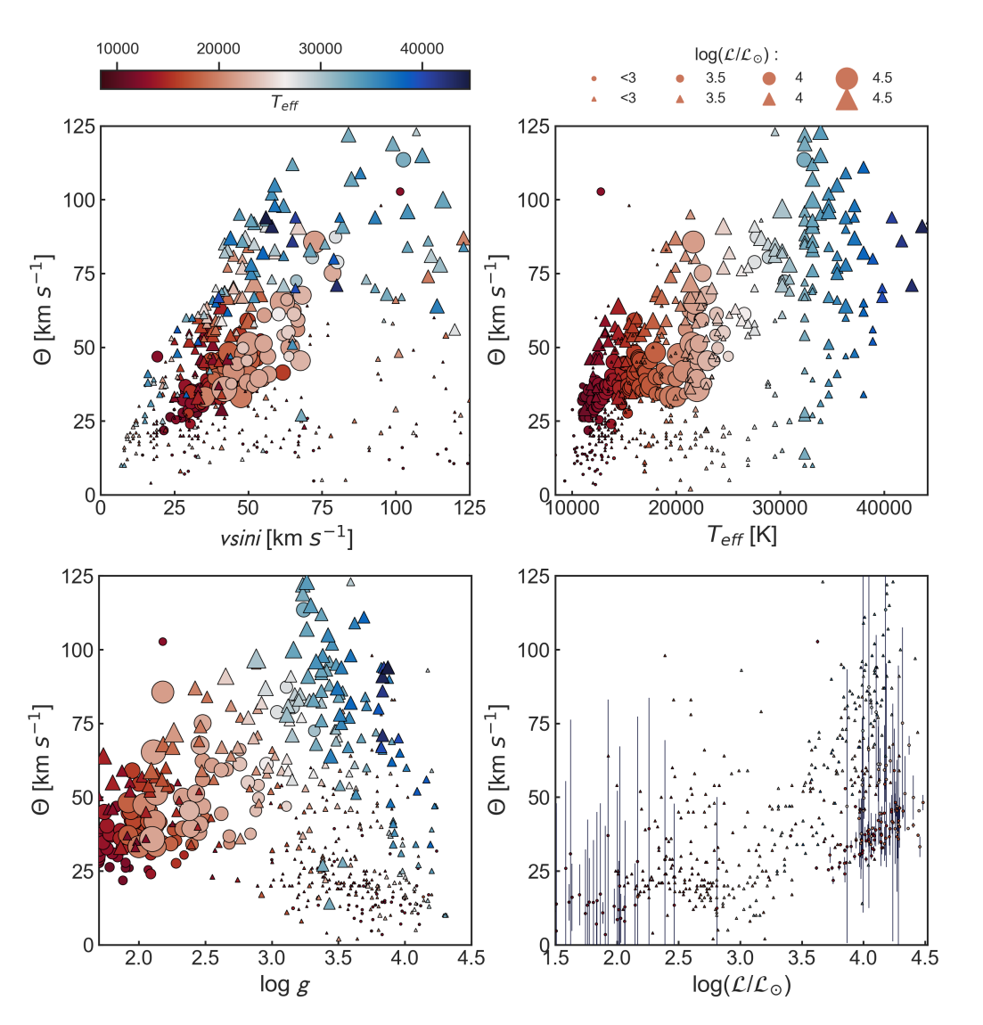
Figure 3: Macroturbulent velocity as a function of stellar parameters. From top left to bottom right:$\Theta$ vs $v\sin i$, $\Theta$ vs $T_{\rm eff}$, $\Theta$ vs $\log g$, and $\Theta$ vs log$\mathcal{L}/\mathcal{L_{\odot}}$. Marker size is proportional to $\mathcal{L}$, colour maps temperature $T_{\rm eff}$. The error bars in the lower right panel are only shown for our measurements as they are not available for the sample of Simón-Díaz et al. (2017).

The macroturbulent velocities $\Theta$ of the full sample are shown as histograms and Kernel Density Estimates (KDE) in Fig.2. The left panel shows the entire sample. The middle panel shows two subsamples separated by metallicity (dashed light grey for the LMC and dark grey for the Galaxy). The right panel shows two subsamples separated by the method of measurement (dashed light grey for the method we applied and dark grey for the one used in Simón-Díaz et al. (2017)), which we treat separately to analyse potential systematic shifts due to methodological differences. One can see three peaks in the distributions around 20 km s^-1, 40 km s^-1, and 60 km s^-1. Their meaning becomes clear when comparing $\Theta$ to the other observables such as temperature and luminosity in Fig.3, where colour shows temperature, symbol size – spectroscopic luminosity, and the symbol itself (circles and triangles) shows whether the measurement originates from us or is taken from Simón-Díaz et al. (2017), respectively. The first and the last peaks of the histograms are only visible in the Galactic subsample and belong to the main-sequence and evolved populations, respectively. This is seen in Fig.3, with the bulk of low-$\Theta$ objects corresponding to low-luminosity and high-$\log g$ at all temperatures. The highest Galactic peak of 60 km s^-1 corresponds to the evolved population with low-$\log g$ and high luminosity at all temperatures. The middle 40 km s^-1 peak originates clearly from the LMC subsample and is analogous to the peak of 60 km s^-1 shifted to lower values due to the difference in the metallicity of the subsamples. There is no second low peak in the LMC subsample since all the observed targets from the LMC fell in the supergiant regime (see left panel in Fig.1).

Another notable feature is visible in the KDE in the right panel of Fig.2. A small shift of the low-$\Theta$ peak occurs between our and Simón-Díaz et al. (2017) measurements of the Galactic main-sequence stars. The same difference may be noticed in the lower right panel of Fig.3 (showing a pairwise plot of $\Theta$ and spectroscopic luminosity) as a slight kink present around 2-2.5 in log$\mathcal{L}/\mathcal{L}_{\odot}$. It is unclear whether the shift is caused by the methodological differences or is due to differences in the parameter region covered by our samples. Our Galactic sample covers masses from 2.5 to 5 $M_{\odot}$, while the sample of Simón-Díaz et al. (2017) starts at 4 $M_{\odot}$, hence the overlap is limited to a few stars only.

The upper left panel of Fig.3 shows relations between projected rotational velocity $v\sin i$  and macroturbulent velocity $\Theta$. One can see qualitatively three populations showing linear growth of $\Theta$ with $v\sin i$ , as noticed by Simón-Díaz et al. (2017), with different slopes for each population. The clear linear trends are likely caused by the ability of the FT method to separate rotational and macroturbulent broadenings, which strongly depends on whether they operate in different frequency ranges of the FT or not. The limitations of the FT approach for measuring rotational velocities are extensively discussed by Aerts et al. (2014) and Serebriakova et al. (2023), thus we restrain from the detailed discussion of this matter. We note though that the FT method has several assumptions. First, it assumes that the total broadening may be represented by a convolution of the rotational profile with all other mechanisms as independent functions. Second, the rotational profile itself is thought to be a simplified function with a fixed linear limb darkening coefficient, which allows for the FT of the rotational profile of a given $v\sin i$  to be characterised by a single parameter – the position of the first zero. Moreover, the position of the first zero in the FT should ideally not overlap features caused by other broadening functions, which implies rotation dominating over all other mechanisms. Lastly, the analysed line profiles must be symmetric. In reality, these assumptions are rarely met and the FT of the line profiles shows several zeros that are smeared out and are thus difficult to interpret. This causes, in our case, high degeneracy between $\Theta$ and $v\sin i$, and leads to the large errors for $\Theta$ in the lower right panel of Fig.3.

In all pairwise plots of Fig.3, the macroturbulent velocities $\Theta$ show the same trends of increasing with temperature and luminosity and decreasing with surface gravity. The $\Theta$ of Galactic stars are systematically higher than those of the LMC stars, although it is not clear whether the difference is caused by the metallicity and not the bias of the LMC sample that is overpopulated with evolved stars.

3 MESA models

A grid of stellar structure and evolution models was computed with the mesa code (Paxton et al. (2011), Paxton et al. (2013), Paxton et al. (2015), Paxton et al. (2018), Paxton et al. (2019), Jermyn et al. (2023)) of version r15140. The chosen input physics is taken from Michielsen et al. (2023), where a detailed description is provided. For convection, we use the Mixing Length Theory (MLT) with a mixing length parameter $\alpha_{MLT}$=2.0. The Ledoux criterion for convection was adopted, with no semi-convection allowed. Michielsen et al. (2023) includes extra core-boundary mixing, implemented as both step-function increase of the core size by a factor $\alpha_{ov}$ (often referred to as step overshooting parameter), and by the exponentially decreasing mixing characterised by $f_{ov}$ parameter. We set these parameters to 0.05 and 0.005, respectively, to keep the extra mixing minimal.

The grid was computed for full mass range in our sample and uniform coverage in the HRD (2, 2.5, 3, 4, 5, 7, 9, 12, 15, 20, 25, 32, 40, 60, and 80 $M_{\odot}$). The evolution was stopped at log$T_{\rm eff}$¿ 3.8 for masses up to 9$M_{\odot}$ and log$T_{\rm eff}$¿ 4.0 for higher masses, which is dictated by the span of our observed parameter ranges.

Fig.4 shows Kippenhahn diagrams for initial masses 60, 20, 12, 7, and 3 $M_{\odot}$ with $Z$=0.014 (while $Z$=0.006 are available in the Appendix A). The radiative transfer zones are hatched, and Ledoux-unstable convective zones are colour-mapped based on convective velocity. The odd panels show the upper 10% of the stellar radius, where one can see the development of subsurface convective layers with age and initial mass, as well as ranges of convective velocity. The latter is near-zero for lower masses and only reaches some 10 km s^-1  late in the post-MS stage, while high mass stars have up to 80  km s^-1  already at the early MS.

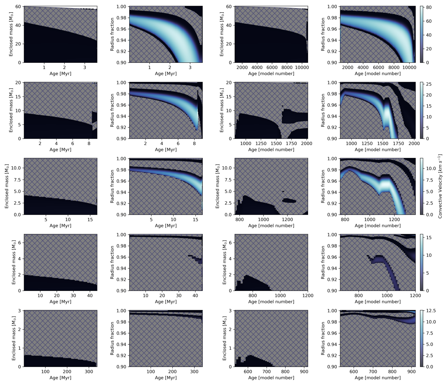
Figure 4: Kippenhahn diagrams for 60, 20, 12, 7, and 3 $M_{\odot}$ (rows) stellar models at metallicity $Z$=0.014. Odd columns – full radius (in mass units), even columns – zoom into the outer 10% of radius (in radius units). Hatched areas denote radiative zones. The Ledoux-unstable convective zones are colour-mapped based on convective velocity. Two left columns are plotted with age in Myr, while two right columns are plotted with age in the model number, which allows a better view of the short-lived post-MS stages.

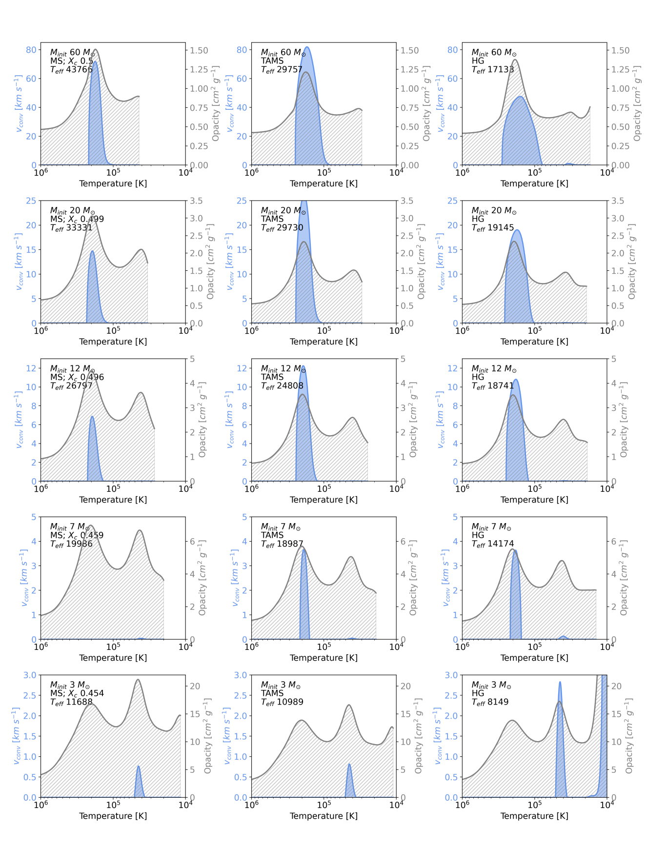
Figure 12: Profiles of opacity (grey) and convective velocity (blue) as a function of temperature. Initial mass varies in rows: 80, 20, 12, 7, and 3 $M_{\odot}$. In columns, three evolutionary stages are presented: MS, TAMS, and Hertzsprung gap. All models are computed for the Solar metallicity $Z$=0.014.

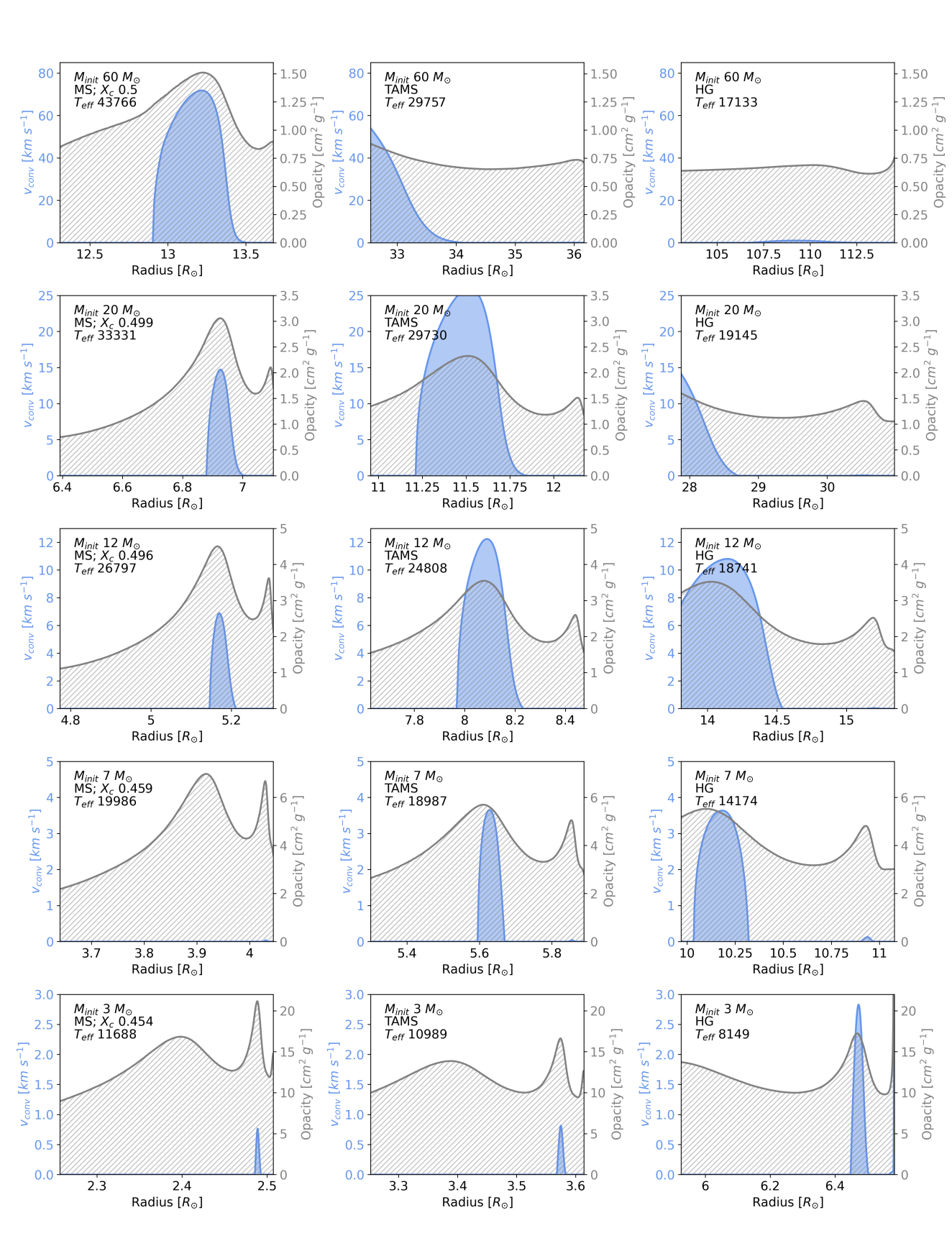
Figure 13: Profiles of opacity (grey) and convective velocity (blue) as a function of radius (zoomed into outer 10% of the radius). The panels are the same as in Fig.12.

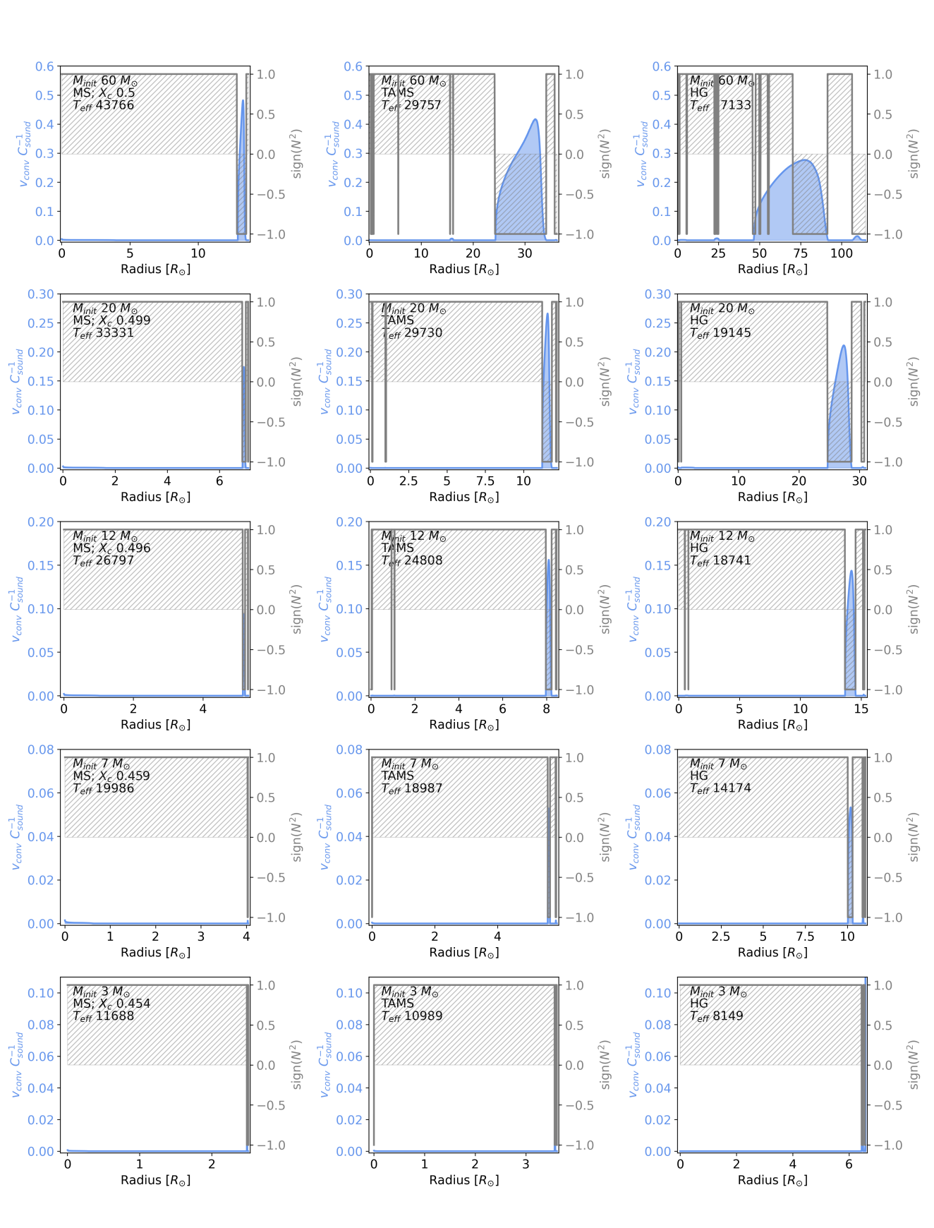
Figure 15: Profiles of the sign of the squared Brunt-Väisälä frequency (grey) and convective velocity as a fraction of sound speed (blue) as a function of radius (full radius). The panels are the same as in Fig.12.

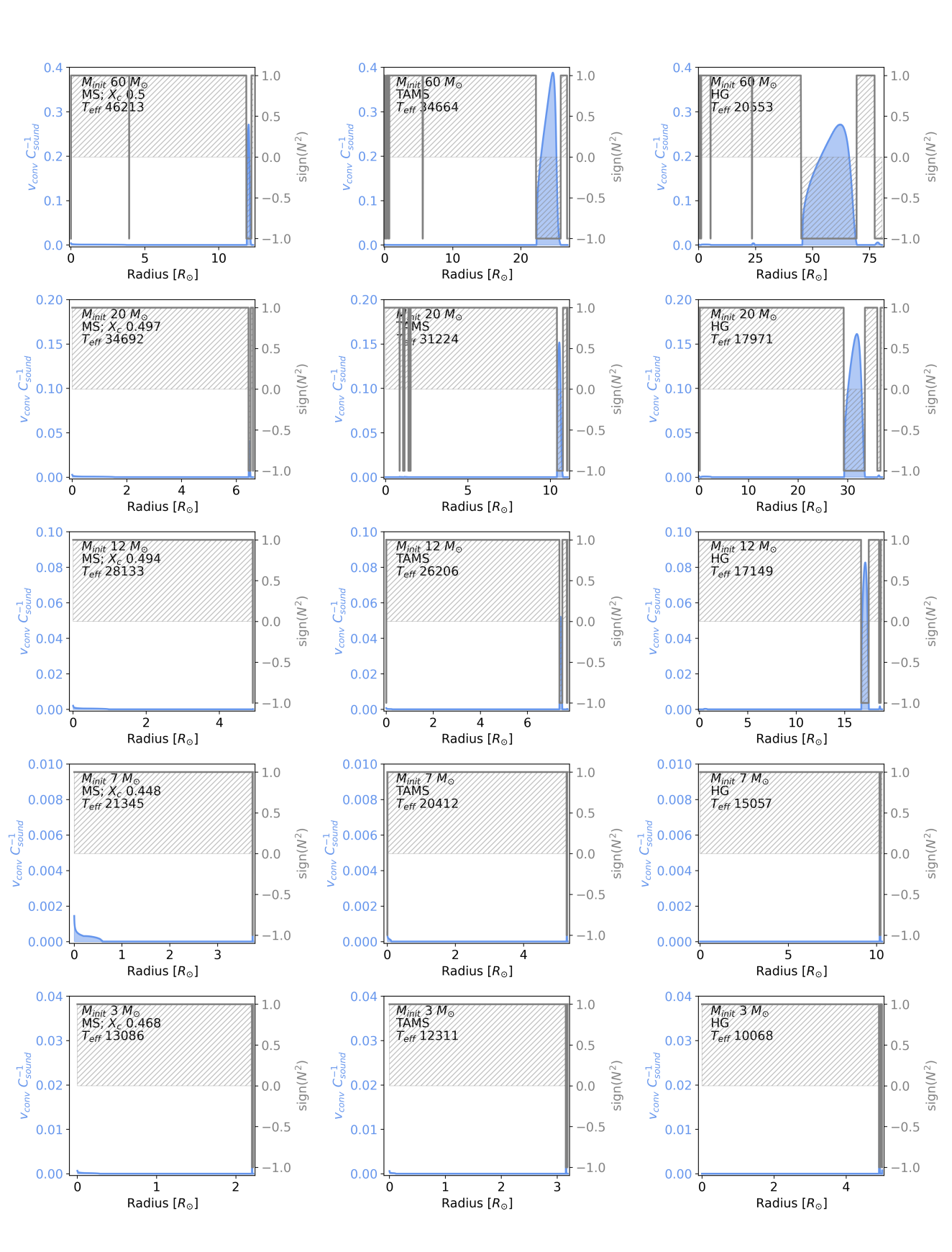
Figure 19: Profiles of the sign of the squared Brunt-Väisälä frequency (grey) and convective velocity as a fraction of sound speed (blue) as a function of radius (zoomed into outer 10% of radius). The panels are the same as in Fig.12 but for $Z$=0.006.

These models are shown in more detail in Figs. 12 and 13 of the Appendix C, where full internal profiles are plotted for three snapshots at three evolutionary stages: mid-MS, TAMS, and HG. While the former plot shows convective velocity and opacity versus temperature, the latter plot shows the same quantities as a function of stellar radius. In Fig. 12, one can clearly see the iron and helium opacity bumps depending on the mass and evolutionary stage, triggering the formation of a convective zone. The iron opacity bump at T $\sim 2\times 10^{5}$ K is responsible for high convective velocities in the high mass regime (7 $M_{\odot}$ and higher). The He ii opacity bump at T $\sim 4\times 10^{4}$ K causes convective velocities at lower masses. It also becomes significant at late stages of evolution for all mass regimes in the expanded envelope, where it forms the second peak in convective velocities with a much smaller amplitude than the iron one. Despite the absolute values of the FeCZ convective velocity are large in some cases, we show that they are subsonic by plotting velocities as a fraction of the sound speed in Figs.15 and 19.

4 Comparing convective velocity and macroturbulent velocity

Figure 5: Convective velocities in the HRD interpolated from MESA models for continuous representation. Top to bottom: metallicity $Z$=0.006 and 0.014. Left to right: convective velocities in the regions of iron and helium opacity bumps. Evolutionary tracks that were used for the interpolation are shown in each panel. Coloured circles show observed macroturbulent velocities measured in this work, triangles those measured in Simón-Díaz et al. (2017).

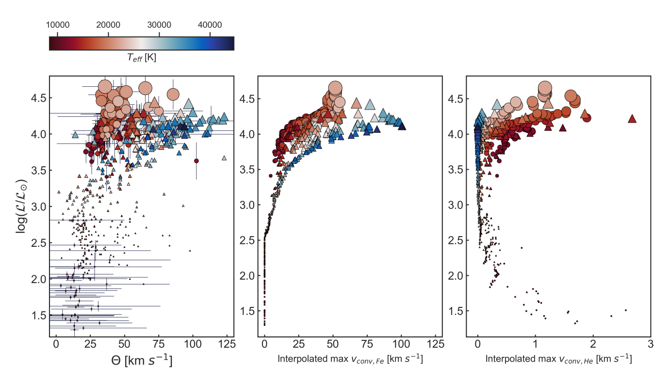
Figure 6: Dependence of the macroturbulent and convective velocities on spectroscopic luminosity of the star. From left to right: observed macroturbulent velocities (left) and predicted with MESA convective velocities for the iron (middle) and helium (right) opacity bumps. Convective velocities in the middle and right panels have been interpolated on the observed positions in the HRD from Fig.5.

Fig.5 shows the distribution of convective velocities in the HRD as predicted by MESA models, separately for the Fe and He opacity bumps. Measurements of the macroturbulent velocity are presented with the coloured symbols (see figure caption for details). It is well visible that convective velocities in the Fe opacity bump have very similar trends as the observed macroturbulent velocities in the high mass regimes ($M>10M_{\odot}$ or $log\mathcal{L}/\mathcal{L_{\odot}}>2.5$) with the same ranges of variation. For the lower masses, the observed macroturbulent velocities have much larger scatter and amplitudes than the convective velocities in both the Fe and He opacity bumps. The same is seen in Fig.6 where the same macroturbulent and interpolated convective velocities are plotted along the x-axis vs spectroscopic luminosity $\log\mathcal{L}/\mathcal{L_{\odot}}>2.5$, while colour maps the effective temperature. The He-bump velocity is too small to explain any observed macroturbulent velocities that are two orders of magnitudes larger. The Fe-bump only appears for stars with $\log\mathcal{L}/\mathcal{L_{\odot}}>2.5$ or $M>10M_{\odot}$. Therefore, we hypothesis that the Fe-bump and macroturbulent velocities are connected in the high-mass regime while there is a lack of such relation for lower stellar masses.

Macroturbulent velocities measured in spectral lines can not be directly fitted by the model convective velocities in the subsurface convection layers since those layers are located much deeper than the line formation region in the photosphere. Note that it is only true for our 1D models, while Schultz et al. (2022, 2023a) showed that the subsurface convection velocities reach the photosphere in their 3D models. Rather, we analyse the possible connection between these two quantities looking at their trends separately from a statistical point of view.

4.1 Multivariate linear regression

As the first step of this analysis, we follow the statistical approach of Aerts et al. (2023) and Serebriakova et al. (2023) and employ multivariate linear regression. Multivariate linear regression is a statistical technique used to model the relationship between two or more predictors (independent variables) and a single predicted (dependent) variable. It extends the concept of simple univariate linear regression, which deals with one predictor and one predicted variable, to accommodate multiple predictors, thereby allowing for a more comprehensive analysis of complex data sets. Multivariate linear regression can be employed to investigate the relationships between stellar parameters and show how various factors simultaneously influence a variable of interest, which is, in our case, macroturbulent velocity $\Theta$. We investigate trends in the observed $\Theta$ quantitatively from multivariate linear regression models in the following form:

$$V=c_{0}+\sum_{i=0}^{N}c_{i}P_{i},$$ (1)

where $V$ is a dependent variable (in our case, macroturbulent velocity $\Theta$), $P_{i}$ – predictors (other observables or model parameters), and $c_{i}$ – coefficients of linear regression for a corresponding $i$-th predictor.

In Serebriakova et al. (2023), based on adjusted $R^{2}$-statistics, 96.4% of variability in the observed macroturbulent velocities of 126 LMC stars were found to be explained by only two predictors: $T_{\rm eff}$ and $v\sin i$, while the set of observables ($T_{\rm eff}$, $\log g$, $\log\mathcal{L}/\mathcal{L}_{\odot}$, and $v\sin i$) was tested and the rest observables were found insignificant for predicting $\Theta$. Due to the absence of any analogue of $v\sin i$ in our non-rotating mesa models, we need to repeat the test of different combinations of predictors without $v\sin i$ to find a set of significant observables that are available in models. In absence of $v\sin i$, we found both $\log g$ and $\log\mathcal{L}/\mathcal{L}_{\odot}$, in addition to log$T_{\rm eff}$, to be significant, although $\log\mathcal{L}/\mathcal{L}_{\odot}$ is computed as $\mathcal{L}=T_{\text{eff}}^{4}/g$. Therefore, we further test all three parameters, $\log\mathcal{L}/\mathcal{L}_{\odot}$, log$T_{\rm eff}$, and $\log g$, as predictors on the observed data. The results of the test are presented in Table 1 as p-values and coefficients $c_{i}$ per each predictor, and adjusted $R^{2}$ per tested dataset.

Table 1: Results of the multivariate linear regression. log$\mathcal{L}/\mathcal{L_{\odot}}$, $T_{\rm eff}$, and $\log g$  were used as predictors and observed macroturbulent velocities as the dependent variable. The rows correspond to different subsets of the data separated by a range of spectroscopic luminosities and by metallicity. $P>|t|$ and $c_{i}$ values for each predictor are given in every cell as top and bottom numbers, respectively. The adjusted $R^{2}$ are given in the last column.

Dataset	$\log\mathcal{L}/\mathcal{L_{\odot}}$	$T_{\rm eff}$	$\log g$	Const	Adj. $R^{2}$
Obs Gal, all $\log\mathcal{L}/\mathcal{L}_{\odot}$	0.000	0.000	0.000	0.000	0.331
	25.72	-15.33	12.00	-9.33
Obs Gal, $\log\mathcal{L}/\mathcal{L}_{\odot}>2.5$	0.000	0.000	0.000	0.000	0.569
	49.73	-37.11	18.11	-20.37
Obs Gal, $\log\mathcal{L}/\mathcal{L}_{\odot}>3.0$	0.000	0.000	0.000	0.000	0.602
	79.08	-68.56	31.23	-36.22
Obs Gal, $\log\mathcal{L}/\mathcal{L}_{\odot}<3.0$	0.310	0.244	0.899	0.322	0.001
	-5.52	9.78	-0.97	4.30
Obs Gal, $\log\mathcal{L}/\mathcal{L}_{\odot}<2.5$	0.568	0.524	0.263	0.477	0.002
	7.30	-11.98	18.78	-6.97
Obs LMC, all $\log\mathcal{L}/\mathcal{L}_{\odot}$	0.002	0.001	0.000	0.000	0.420
	20.67	-21.48	28.72	-12.75

We repeated the exercise for various subsamples with cut-off by $\log\mathcal{L}/\mathcal{L}_{\odot}$ in order to look at behaviour of the measured microturbulent velocities in different luminosity regimes. These regimes are evident in Fig.6 where a turn of $\Theta$ is seen towards higher values above $\log\mathcal{L}/\mathcal{L}_{\odot}$ = 2.5. For the LMC sample, we only use the full sample as all stars in that sample already have $\log\mathcal{L}/\mathcal{L}_{\odot}$ ¿ 3. In Table 1, one can see how the fraction of explained variance (reflected in adjusted $R^{2}$) increases for subsamples with higher $\log\mathcal{L}/\mathcal{L}_{\odot}$, and reaches 60%. Moreover, the samples that only include stars with $\log\mathcal{L}/\mathcal{L}_{\odot}$ ¡ 3 show large p-values and near-zero $R^{2}$, suggesting the predictors fail to explain variability in $\Theta$ for low-$\log\mathcal{L}/\mathcal{L}_{\odot}$ subsample.

Furthermore, we can compare the roles of each predictor in explaining observed $\Theta$ with the roles of the same predictors in explaining model convective velocities $v_{conv}$ by looking at their coefficients. We repeated the same multivariate linear regression for the model sample, using each computed internal profile as a point of a sample with model $v_{conv}$ as the dependent variable. First, we repeated tests of sets of predictors for their predicting power (which are not limited by a modest set of observables that we have to stick to with observed data). While it appeared possible to describe up to 96% of variability using model predictors such as age and mass (as expected), a subset of observable parameters had to be selected for qualitative comparison with observations. Same $\log\mathcal{L}/\mathcal{L}_{\odot}$, log$T_{\rm eff}$, and $\log g$ were found to all be significant and explain up to 79% of variability in the model subsets. The results of multivariate linear regression of the model data are presented in the Appendix B in Tables 4 and 5 as the model data provided more possible subsets. The subsets include both metallicities with full coverage of the parameter space, convective velocity in both iron ($v_{\rm conv,Fe}$) and helium ($v_{\rm conv,He}$) convective layers, as well as maximum ($v_{\rm conv,x}^{\rm max}$) or integrated velocity ($v_{\rm conv,x}^{\rm integr}$) chosen as dependent variable.

The higher adjusted $R^{2}$ values in the model data compared to observations (for example of $v_{\rm conv,Fe}^{\rm max}$ subsets with $\log\mathcal{L}/\mathcal{L}_{\odot}$ ¿ 3, $R^{2}$ is 0.794 against 0.602 for the Solar metallicity, or 0.722 against 0.420 for the LMC metallicity) suggest additional complexities (rotation) or observational uncertainties (in both the position in HRD and measured $\Theta$) in the observed datasets. The overall consistency in coefficient trends between the model and observed datasets for each predictor suggests that the fundamental physical relationships between the predictors and the $v_{\rm conv,Fe}^{\rm max}$ and $\Theta$ are similar. The similar coefficient trends across different luminosities and metallicities also indicate that the predictors $\log\mathcal{L}/\mathcal{L}{\odot}$, $T_{\rm eff}$, and $\log g$ play comparable roles in influencing both macroturbulent and convective velocities, which was seen in Fig. 5 and 6. The largest discrepancies are found in low-$\log\mathcal{L}/\mathcal{L}_{\odot}$, where model dataset have near-zero $v_{\rm conv,Fe}^{\rm max}$ or $v_{\rm conv,He}^{\rm max}$ with no scatter, while observations have a large scatter around still noticeable velocities with weak to no trends with other observables.

The comparison of all tests shows that the observed scatter in macroturbulent velocities $\Theta$ for the low-mass regime ($\log\mathcal{L}/\mathcal{L}_{\odot}$ ¡ 3 or $M<12M_{\odot}$) can not be explained by same predictors that partially describe model convective velocities. For high-mass regime ($\log\mathcal{L}/\mathcal{L}_{\odot}$ ¿ 3 or $M>12M_{\odot}$) and Solar metallicity, 60.2% of the observed $\Theta$ variability is explained by the same predictors and similar coefficients as Fe-bump convective velocities, pointing to the common origin of the two phenomena. Even though it is noticeably less than 79.4% described in the model convective velocities, the observed sample has a scatter due to the measurement errors that smear out the trends. Moreover, the coefficients of all predictors show consistently similar trends with luminosity and metallicity, which illustrates that the predictors play comparable roles in influencing both macroturbulent and convective velocities in the observations and models, respectively.

4.2 Principal Component Analysis

Principal Component Analysis (PCA) is a statistical technique widely utilised in the context of multivariate data analysis to investigate the underlying structure and trends within high-dimensional datasets. PCA operates by transforming the original n-dimensional data into a new coordinate system where the axes (principal components) are ordered by the amount of variance they capture from the data. The first principal component captures the maximum variance, the second captures the second most variance, and so on. This transformation is achieved through an eigenvalue decomposition of the covariance matrix of the data, yielding eigenvalues and eigenvectors that define the principal components.

In the context of comparing two n-dimensional point clouds, PCA can be applied separately to each dataset to derive their respective principal components. By examining the principal components, we can compare the direction and magnitude of the variance captured in each dataset. Specifically, if the principal components of both clouds align similarly (i.e., they have similar eigenvectors and eigenvalues), it suggests that the two datasets share similar trends. Conversely, significant discrepancies in the principal components would indicate divergent trends between the two point clouds.

In order to compare the trends in $\Theta$ and $v^{\rm max}_{\rm conv,Fe}$, we independently apply PCA to four clouds of points: observed LMC, model LMC, observed Galactic, and model Galactic datasets. In each case, we used same variables, with the difference that $\Theta$ and $v^{\rm max}_{\rm conv,Fe}$ were only used in the observed and model data, respectively, so the full list of dimensions per each point in the cloud consisted of $T_{\rm eff}$, $\log g$, log$\mathcal{L}/\mathcal{L_{\odot}}$, and either $\Theta$ or $v^{\rm max}_{\rm conv,Fe}$. We included the first two components only since they provided cumulative explained variances of 89 to 95 % in each of the four datasets, as with the ratio per component shown in Table 2.

Table 2: Explained Variance Ratios and Cumulative Explained Variance

	LMC Obs		LMC Model		Gal Obs		Gal Model
	PC1	PC2	PC1	PC2	PC1	PC2	PC1	PC2
Explained Variance Ratio	0.6487	0.2429	0.5680	0.3857	0.5507	0.3756	0.6063	0.3472
Cumulative Explained Variance	0.6487	0.8916	0.5680	0.9536	0.5507	0.9263	0.6063	0.9535

Each principal component may be represented as a linear combination of the initial set of parameters ($T_{\rm eff}$, $\log g$, log$\mathcal{L}/\mathcal{L_{\odot}}$, and either $\Theta$ or $v^{\rm max}_{\rm conv,Fe}$). The coefficients for each parameter in each principal component for each dataset are provided in the Table 3. Comparison of these coefficients for four datasets allow us to draw the following conclusions. The primary component (PC1) shows consistent contributions from all parameters across all datasets, indicating that the primary trend is similar in both observations and models. The coefficients for $v^{\rm max}_{\rm conv,Fe}$ and $\Theta$ are comparable, suggesting these parameters are interchangeable in capturing the primary trend. However, the secondary component (PC2) exhibits significant differences in both the sign and magnitude of the coefficients for most parameters. These discrepancies may be attributed to specifics of the observed sample, such as uncertainties, presence of extra parameter $v\sin i$, that is absent in the models, and limited sample size and parameter span.

Table 3: Principal Component Loadings and Correlations

Variable	LMC Obs		LMC Model		Gal Obs		Gal Model
	PC1	PC2	PC1	PC2	PC1	PC2	PC1	PC2
Loadings
$T_{\text{eff}}$	0.6052	0.0236	0.5786	-0.3787	0.5060	-0.5168	0.5835	-0.3338
$\log g$	0.5505	-0.3848	0.4407	-0.5961	-0.0594	-0.8095	0.3568	-0.7008
$\log(\mathcal{L}/\mathcal{L_{\odot}})$	0.2604	0.9191	0.4614	0.5394	0.6103	0.2653	0.4794	0.5217
$\Theta$	0.5127	-0.0814			0.6065	0.0849
$v_{\text{conv, Fe}}^{\text{max}}$			0.5080	0.4586			0.5500	0.3540
Correlations
$T_{\text{eff}}$	0.9749	0.0233	0.8721	-0.4703	0.7510	-0.6335	0.9086	-0.3934
$\log g$	0.8868	-0.3793	0.6643	-0.7404	-0.0882	-0.9922	0.5556	-0.8259
$\log(\mathcal{L}/\mathcal{L_{\odot}})$	0.4194	0.9059	0.6955	0.6700	0.9059	0.3252	0.7465	0.6149
$\Theta$	0.8259	-0.0802			0.9002	0.1041
$v_{\text{conv, Fe}}^{\text{max}}$			0.7657	0.5695			0.8565	0.4172

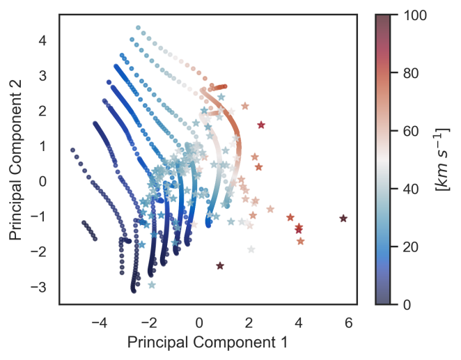
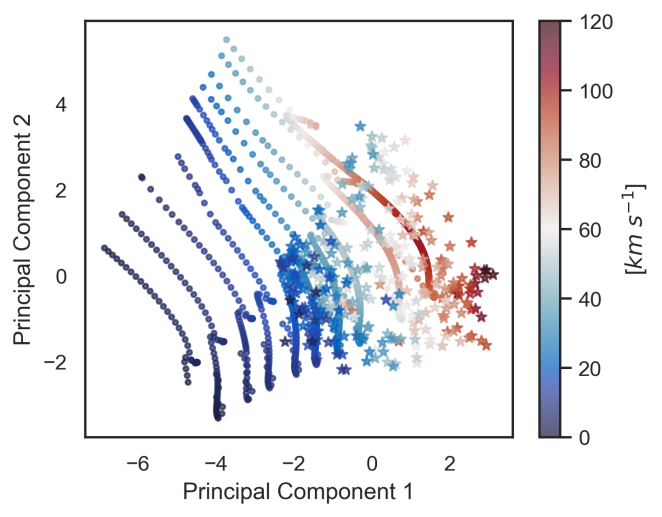
Figure 7: Datasets projection on the principal components space. Left panel – models with $Z$=0.006 (circles) and observed LMC sample (stars), right panel – models with $Z$=0.014 (circles) and observed Galactic sample (stars). Colour shows convective velocity for the model data and macroturbulent velocities for the observed data. All the four datasets were analysed independently.

The visual representation of all four datasets in PC1-PC2 space is shown in Fig.7, where circles represent model data points, and stars represent observational data points. The colour indicates the value of $\Theta$ for observations and $v^{\rm max}_{\rm conv,Fe}$ for models. Although the four datasets were analysed independently, they align very similarly in the PC1-PC2 space. The alignment of points and matching colour gradients strongly indicate that the primary trend is consistent across all four datasets. This suggests that the underlying structure and trends in the full 4-dimensional clouds are captured similarly by the first principal component across all datasets, supporting the hypothesis of $\Theta$ and $v^{\rm max}_{\rm conv,Fe}$ playing the same role in forming the trends. On the contrary, if we compare how the observed sample is misaligned from model tracks (compared to how the plot looks in the HRD instead of PC1-PC2), we can see obvious stretch and shrink of spans of the observed samples. Looking at the Galactic sample (second panel in Fig.7), one can see the shift and shrink of the observed sample while matching colours. The shift indicates systematic differences in absolute values of $\Theta$ and $v^{\rm max}_{\rm conv,Fe}$ with the former being systematically higher. The shrink of the cloud to match lower-masses observations with higher-masses tracks indicates that the observed $\Theta$ in lower-mass regime is inconsistent with near-zero convective velocities of the models, while high-mass observed points are kept aligned with high-mass tracks. We interpret this as a support for the hypothesis of having two principally different regimes, with $\Theta$ in high- and low-mass regimes caused by different mechanisms. The LMC sample, in contrast to the Galactic sample, seems to be stretched compared to model tracks and misaligned in colour, which we interpret to be caused by the small sample size in a very limited span of masses, while the Galactic sample covers the full range of parameters.

5 On wave tunnelling through subsurface convective layers

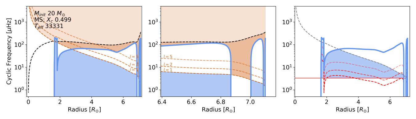
Figure 8: Propagation diagram for a 20 $M_{\odot}$ main-sequence star model. The x-axis represents the radius in solar radii, y-axis shows the cyclic frequency in microhertz. The left and right panels show full radius, while the middle panel shows the external 10% of radius. The blue line represents the Brunt-Väisälä frequency $N$, the brown dashed lines correspond to the Lamb frequencies $S_{l}$ for different spherical harmonic degrees $l$, and the black dashed line shows acoustic cut-off frequency. The blue-shaded region shows the g-mode cavity, and the brown-shaded region – p-mode cavity. The right panel shows profiles of tunnelling $\omega_{min}$ for $l$=1,2,5 in dashed red lines and one horizontal value of $\omega_{min}$ taken near the convective layer (see text for details).

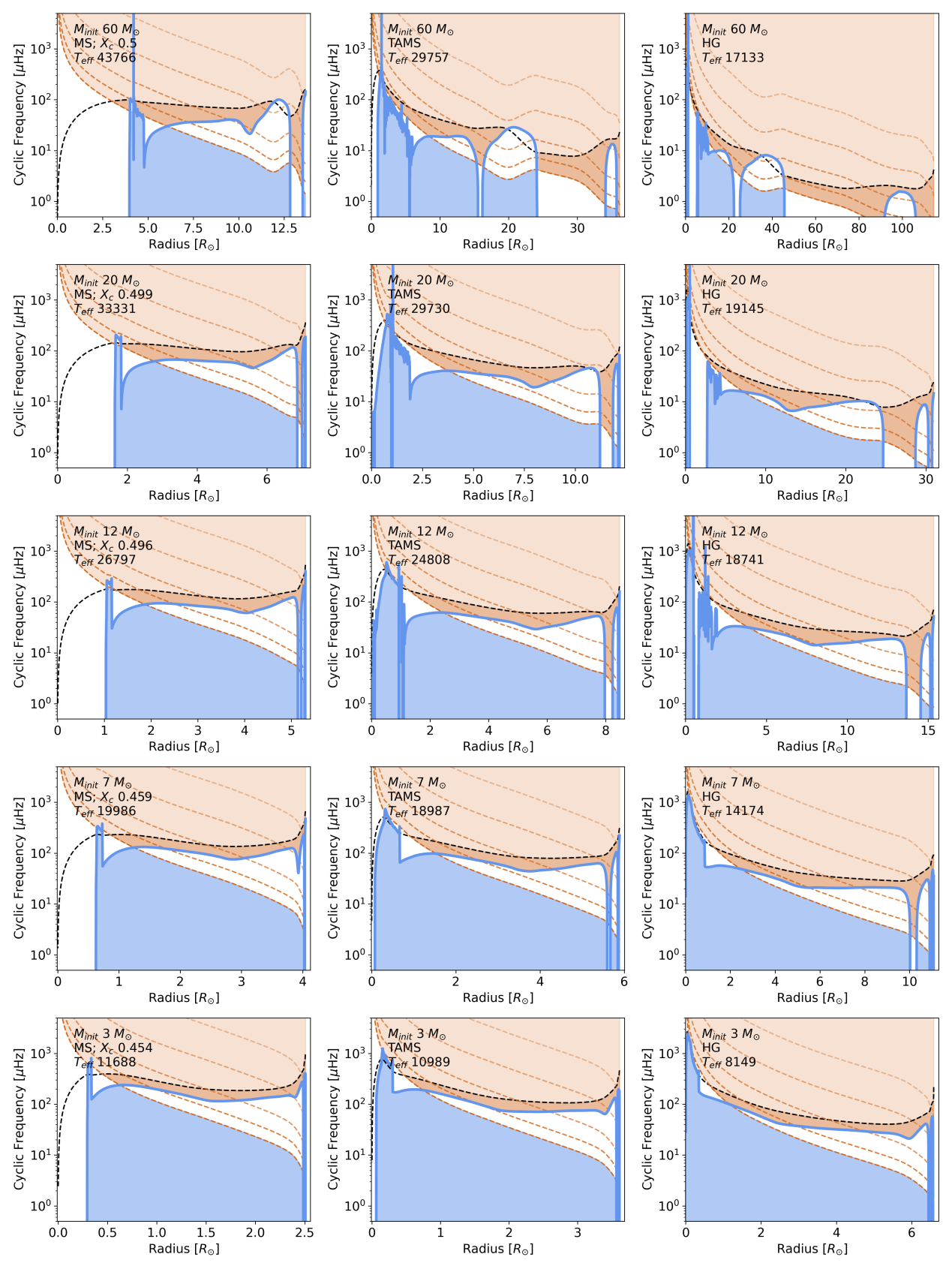
Figure 20: Propagation diagram for masses 80, 20, 12, 7, and 3 $M_{\odot}$ varying with rows. In columns, three evolutionary stages are presented: MS, TAMS, and Hertzsprung gap. $Z$=0.014. The x-axis represents the radius in solar radii, y-axis shows the cyclic frequency in microhertz. The blue line represents the Brunt-Väisälä frequency $N$, the brown dashed lines correspond to the Lamb frequencies $S_{l}$ for different spherical harmonic degrees $l$, and the black dashed line shows acoustic cut-off. The blue-shaded region shows the g-modes cavity, and the brown-shaded region – the p-modes cavity.

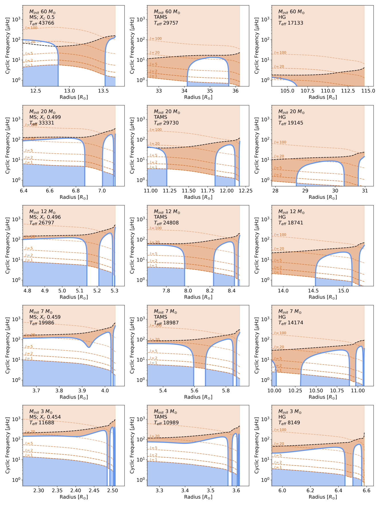
Figure 21: Same as Fig.20, but zoomed in external 10% radius.

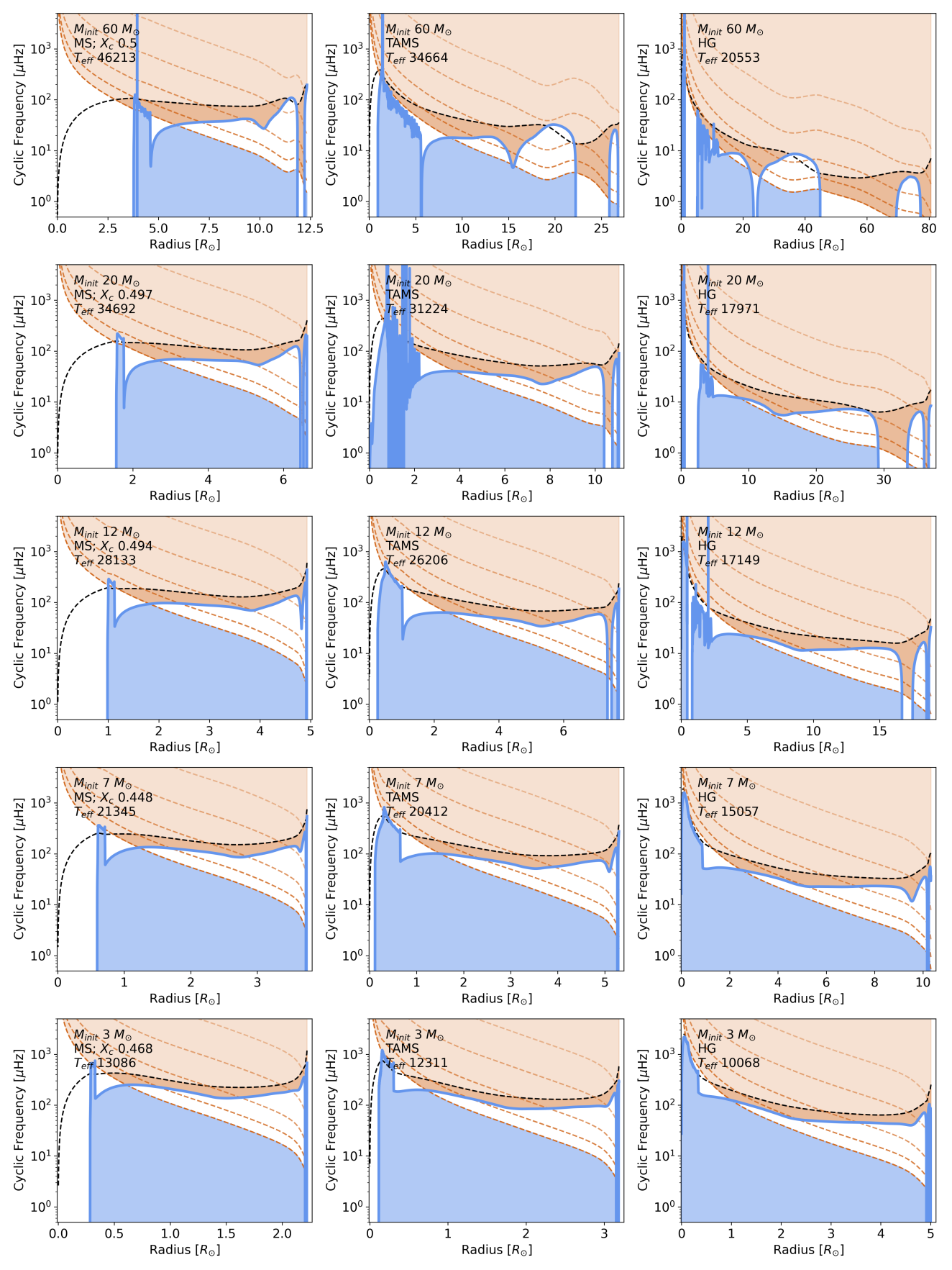
Figure 23: Same as Fig.20, but for $Z$=0.006.

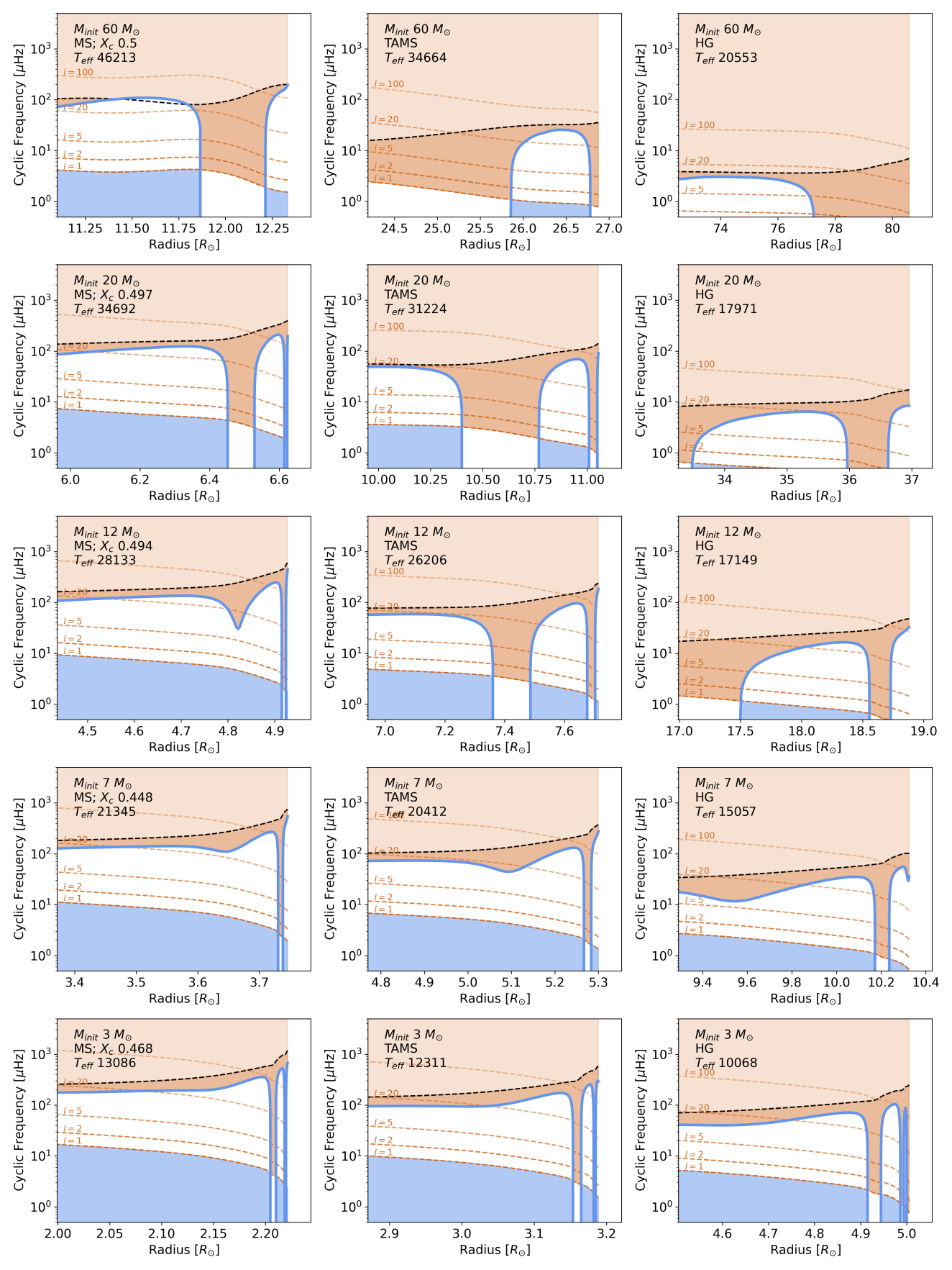
Figure 24: Same as Fig.20, but for $Z$=0.006 and zoomed in external 10% radius.

Model internal profiles computed with mesa allow us to look into the wave propagation by comparing the Brunt-Väisälä $N$ and Lamb $S_{l}$ frequencies across the stellar radius. The first two panels of Fig.8 show an example of such a propagation diagram, i.e. internal profiles of $N$ and $S_{l}$ for a 20 $M_{\odot}$ main-sequence star model at the Solar metallicity. The blue line shows $N$, dashed brown lines – $S_{l}$ for $l$=1,2,5, and black dashed line – the acoustic cut-off frequency. The left panel shows the full radius, and the middle one – zoom-in into the outer 10% of the envelope. The blue-shaded area indicates regions where g-modes and IGW can propagate. This region is defined by frequencies $\omega$ less than both $N$ and $S_{l}$ and where $N^{2}$ is positive (in radiative layers, as negative corresponds to convective layers where g-modes cannot propagate). The brown shaded area shows regions where acoustic modes and waves can propagate, which is defined by frequencies $\omega$ greater than both the Brunt-Väisälä frequency and the Lamb frequency, but less than the acoustic cut-off frequency. Finally, the white regions where $N$ ¡ $\omega$ ¡ $S_{l}$ or $S_{l}$ ¡ $\omega$ ¡ $N$ represent evanescent zones, where waves exponentially decay. In this particular model, one can see present g-mode and p-mode cavities between the core boundary at 2 $R_{\odot}$ and iron-bump convective zone FeCZ at some 6.85 $R_{\odot}$, as well as some between the upper boundary of the FeCZ and the lower boundary of the HeCZ. However, a combination of the extensive FeCZ between 6.85 and 7 $R_{\odot}$ with rapidly decreasing $S_{l}$ and next HeCZ right below the surface does not leave any potential $\omega$ from g-modes or p-modes cavities that could reach the surface. The same propagation plots for models of different masses and evolutionary states are provided in Appendix D (Figs. 20 and 21 for the Solar metallicity and Figs. 23 and 24 for the LMC metallicity).

As a useful addition to the propagation diagrams, we can roughly estimate the minimal wavelength a wave must have to tunnel through the subsurface convective layers before being decayed. The minimal requirement of the wavelength $\lambda$ being larger than the span of the region we want the waves to tunnel through be expressed through wavenumber $k$ as:

$$\lambda=\frac{2\pi}{|k|}.$$ (2)

The frequency $\omega$ is connected to the wavenumber through the dissipation relation of IGW (Aerts et al. (2010)):

$$\omega^{2}=\frac{k_{h}^{2}N^{2}}{k_{r}^{2}+k_{h}^{2}}.$$ (3)

Here, $k_{h}$ and $k_{r}$ are the radial and horizontal components of wavenumber $|k|^{2}=k_{r}^{2}+k_{h}^{2}$

The horizontal wavenumber $k_{h}$ can be expressed in terms of the spherical harmonic degree $l$ and radius $r$ as:

$$k_{h}=\sqrt{\frac{l(l+1)}{r^{2}}}.$$ (4)

The condition $\lambda$ ¿ $r_{2}-r_{1}$, where $r_{1}$ and $r_{2}$ are the positions of lower and upper boundaries of a convective layer, gives the minimal frequency allowing IGW to tunnel through the evanescent zone.

$$\omega_{min}=\frac{(r_{2}-r_{1})N(r)\sqrt{l(l+1)}}{2\pi r}.$$ (5)

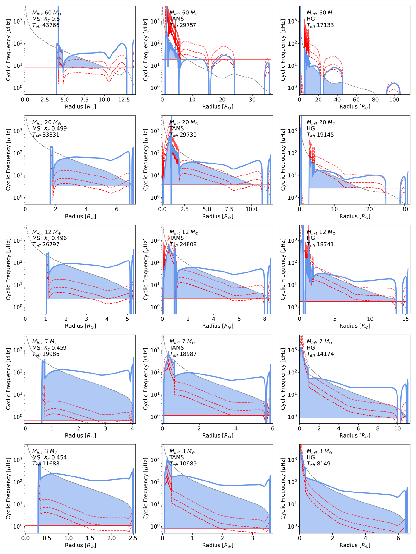
Figure 22: Same as Fig.20, but with tunnelling frequency introduced as red cut-off line.

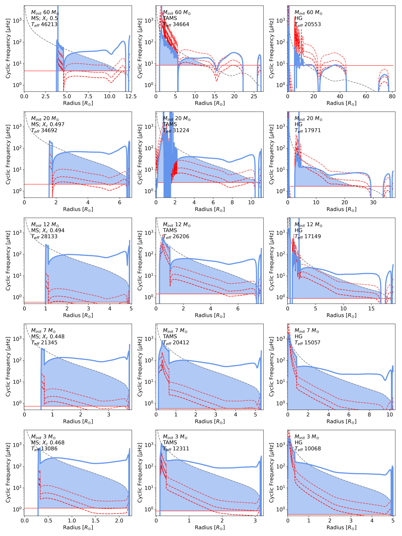
Figure 25: Same as Fig.20, but for $Z$=0.006 and tunnelling frequency introduced as red cut-off line.

The last equation shows that ’tunnelling’ frequency follows the profile of the Brunt-Väisälä frequency scaled by relations of $r_{2}-r_{1}$ and radius $r$, for degrees $l$. The right panel of Fig.8 shows internal profile $\omega_{min}$ for $l$=1,2,5 as red dashed lines, where the span of FeCZ was taken as $r_{2}-r_{1}$. A single minimum may be taken as a value of the $\omega_{min}$ profile for $l$=1 at a point before the convective zone and is shown in the same figure as a solid red horizontal line. This gives a minimal value for a frequency below which waves from below the convective layer can not tunnel through the evanescent zone. This may serve as an additional constraint for the g-mode cavity, extending the condition $\omega$ ¡ $N$ ¡ $S_{l}$ into $\omega_{min,l=1,r=r1^{*}}$ ¡ $\omega$ ¡ $N$ ¡ $S_{l}$. Frequencies satisfying this condition occur in the blue-shaded regions in the right panel of Fig. 8. Same modified propagation diagrams with ’tunnelling’ $\omega_{min}$ for models of different masses and evolutionary states are provided in the appendix D (Figs. 22 and 25 for the Solar and LMC metallicities, respectively). Note that $r_{2}-r_{1}$ was considered individually for each model based on which subsurface convective layer is the most extended for a given mass and age, i.e. the most restrictive on $\lambda$. Such a definition also allows us to introduce a flag for each model depending on the extent of the blue-shaded region between the core boundary and the lower boundary of the thickest convective layer. In other words, if a certain model does not allow any $\omega$ satisfying $\omega_{min,l=1,r=r1^{*}}$ ¡ $\omega$ ¡ $N$ ¡ $S_{l}$ due to $r_{2}-r_{1}$ requiring $\omega_{min}$ ¿ $N$ (or ¿ $S_{l}$), we can flag such a model as forbidding IGWs to tunnel through to the surface. Note that such a crude definition of $\omega_{min}$ makes it rather conservative and may only be used to mark models that forbid tunnelling, but not to saying that the rest of the models allow for it.

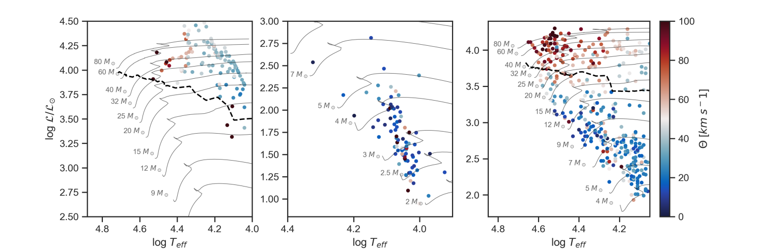
Figure 9: The observed sample with panels as in Fig.1: left - for the LMC sample and metallicity, middle and right - for the Galactic samples and Solar metallicity. Colour shows observed macroturbulent velocities $\Theta$. The thick dashed black line separates the region of forbidden tunnelling (above the line) through subsurface convective layers (see text for details).

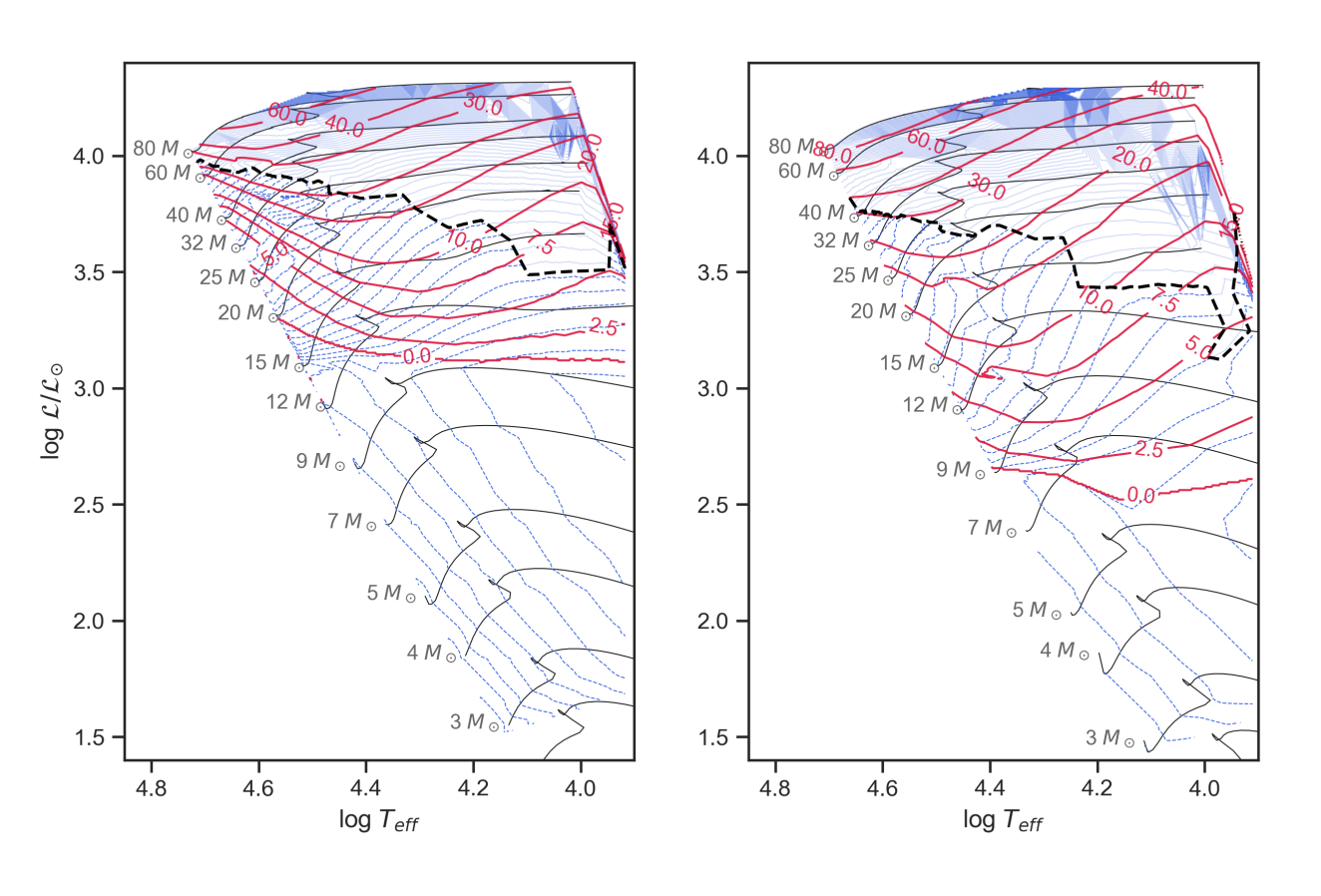
Figure 10: Level-plot of FeCZ maximal convective velocities in solid red lines and tunnelling frequency $\omega_{min}$ in dashed blue lines (see text for details). The thick dashed black line separates the region of forbidden tunnelling (above the line) through subsurface convective layers.

Based on the above definition of models with forbidden tunnelling, we may define corresponding regions in the HRD and compare them with the observed sample. Fig.9 shows the full observed sample in the HRD with colour representing observed macroturbulent velocities $\Theta$ on top of evolutionary tracks. A thick black dashed line defines a boundary between models that forbid tunnelling of core-excited IGWs through subsurface convective layers (above the line) and the models not forbidding it (below the line). One can see that the vast majority of observed high-macroturbulence stars lie above the line, where tunnelling is not possible. This is a strong evidence against core-generated IGWs being responsible for high macroturbulent velocities observed in blue supergiants. This region occurs above 40 $M_{\odot}$ at ZAMS, 20 $M_{\odot}$ at TAMS, and 12 $M_{\odot}$ in the Hertzsprung gap for the Solar metallicity, and above 60 $M_{\odot}$ at ZAMS, 32 $M_{\odot}$ at TAMS, and 12 $M_{\odot}$ in the Hertzsprung gap for the LMC metallicity. in all these cases, the FeCZ is extended enough to block waves from the inside. These cases also have convective velocities up to 80 km s^-1, sufficiently large to describe the high observed macroturbulent velocities (see maps of convective velocities in Fig.5, level-plots in Fig.10 or in Appendix E).

While the region in the lower HRD below the dashed line lacks truly high-macroturbulent stars (except several outliers), the observed microturbulent velocities almost never fall below 20 km s^-1. In the same region, models predict (near-)zero convective velocities (see Fig.10, rendering the FeCZ unlikely to cause the observed macroturbulent broadening, yet allowing for core-generated IGWs to tunnel through the subsurface convective layers. This justifies a regime of core-generated IGWs causing moderate macroturbulence for the stars with initial mass below some 12 $M_{\odot}$.

Finally, the region between 12 $M_{\odot}$ and the dashed line allows for both regimes to co-exist. This co-aligns with the spectroscopic luminosity log$\mathcal{L}/\mathcal{L_{\odot}}$ around 3.5, where we can as well see a sharp turn in the distribution of the observed macroturbulent velocities towards the highest values in Fig.6.

6 Discussion and Conclusions

In this study, we investigated the physical origin of macroturbulent spectroscopic line broadening in hot massive stars by analysing a comprehensive sample of 594 stars with masses ranging from 2.5 to 80 $M_{\odot}$ across two different metallicity regimes: the Large Magellanic Cloud (LMC) and the Galaxy with $Z$=0.006 and $Z$=0.014, respectively. Our sample included 86 stars with macroturbulent broadening measured for the first time. Our study was supplied with a grid of mesa stellar structure models to examine the properties of subsurface convective zones. These models also allowed us to explore wave propagation and the potential for IGWs to tunnel through subsurface convective layers.

To understand the underlying mechanisms behind the macroturbulent broadening, we performed several analyses. We used multivariate linear regression to identify significant predictors in both macroturbulent velocities and convective velocities predicted by models. The analyses showed that in the low-mass regime ($\log\mathcal{L}/\mathcal{L}_{\odot}$ ¡ 3 or $M<12M_{\odot}$), macroturbulent velocities $\Theta$ can not be explained by same predictors that describe model convective velocities. At higher masses and luminosities ($\log\mathcal{L}/\mathcal{L}_{\odot}$ ¿ 3 or $M>12M_{\odot}$), the observed $\Theta$ variability may be largely explained by the same predictors and similar coefficients as FeCZ velocities. The coefficients of all predictors in this high-mass regime show consistently similar trends with luminosity and metallicity, which towards a common origin of the observed macroturbulent and model convective velocities.

We also conducted a Principal Component Analysis (PCA) to compare trends between the observed and model datasets. We found that the underlying structure and trends are captured similarly by the first principal component across independently analysed observed and model datasets. In the high-mass regime, the clouds of the observed and model points align in PC1-PC2 space. On the contrary, in the low-mass regime, they are misplaced, showing that model values fail to predict the observed $\Theta$.

We interpret the consistent results of both PCA and multivariate linear regression as a strong statistical evidence that macroturbulent velocities in stars in different mass regimes are caused by different mechanisms. In stars with initial masses larger than 12 $M_{\odot}$ (or spectroscopic luminosities log$\mathcal{L}/\mathcal{L_{\odot}}$ ¿ 3), macroturbulent velocities are closely related to the convective velocities in the subsurface convection zones formed due to the iron opacity bump (FeCZ), as originally proposed by Cantiello et al. (2009). At the same time, our analysis revealed a clear dependence of macroturbulent velocities on metallicity. In particular, Galactic stars (higher metallicity) exhibited systematically higher macroturbulent velocities compared to stars in the LMC (lower metallicity). This result aligns well with the model predictions: sub-surface convection zones are found to develop at both Galactic and LMC metallicities, albeit magnitude of the convective velocities is generally lower in the latter case.

Since in all our 1D models the regions of FeCZ are situated much deeper than line formation region in the photosphere, it is likely that the surface macroturbulent velocities are formed by IGWs excited at the boundary of FeCZ. Excitation of IGWs by the FeCZ in massive stars has hardly been studied in multi-D simulations. However, Rogers et al. (in preparation; private communication) show that such a subsurface convection zone can generate low frequency waves which reach the stellar surface, in conjunction with higher frequency IGWs generated by core convection. In 3D models computed by Schultz et al. (2022, 2023a) though, the subsurface convection layers expand further than in 1D models and cause turbulent surface with velocities ranges matching observed macroturbulent velocities. However, such simulations are computationally demanding, hence were computed for several snapshots in time and a few values of stellar mass. More simulations would be required to draw definitive conclusions as to whether the subsurface convection could in full explain the observed macroturbulent broadening.

For stars with initial masses below 12 $M_{\odot}$, the convective velocities in both the FeCZ and (HeCZ) are not sufficient to explain the observed macroturbulent velocities, which, although smaller than in higher mass stars, are still significant. This points to the presence of some other mechanism that is responsible for the observed line broadening in these intermediate-mass stars. This may be seen as the change in the distribution of $\Theta$ with luminosity in Fig. 6.

Our analysis of wave propagation through model stellar interiors indicated that core-generated IGWs are highly unlikely to tunnel through extensive subsurface convection layers of stars with initial masses above $\sim$30 $M_{\odot}$. The models from the same region in HRD also have convective velocities up to 80 km s^-1, sufficiently large to describe the high observed macroturbulent velocities. We conclude that macroturbulent velocities are fully determined by the FeCZ properties in this high-mass regime.

The region in the HRD characterised by the initial masses below some 12 $M_{\odot}$ generally lacks stars with high macroturbulent velocity values. At the same time, only a few stars in that region show macroturbulent velocities below 20 km s^-1. In the same region, models predict (near-)zero convective velocities, as seen in Fig.10, rendering the FeCZ unlikely to cause the observed macroturbulent broadening but, at the same time, allowing the core-generated IGWs to tunnel through the subsurface convective layers. This justifies a regime of core-generated IGWs causing moderate macroturbulence for the stars with initial mass below some 12 $M_{\odot}$.

Lastly, the region between 12 $M_{\odot}$ and 30 $M_{\odot}$ allows IGWs to propagate to the surface and at the same time has still large FeCZ convective velocities, meaning the possible region of coexistence of the two mechanisms. More detailed 3D modelling is required to investigate the interplay of subsurface convective layers and core-generated IGWs to determine a more physical estimation of the boundary between the two discussed regimes.

The conclusion on the existence of different regimes aligns with the recent research of the stochastic low-frequency variability from space-based photometry in SMC, LMC, and the Galaxy (Bowman et al. 2024, in preparation). The authors conclude that FeCZ plays different roles based on age, and is only crucial for evolved stars. We draw similar conclusions, but emphasise the importance of the mass range apart from the age, as for the higher masses the FeCZ is extensive from the very ZAMS. Moreover, Bowman et al. (2024, in preparation) present a convection stability window based on Rayleigh number that aligns with our region where IGWs are allowed to tunnel through FeCZ. Furthermore, the authors demonstrate a lack of dependence of the observed SLFV characteristics on the metallicity of the star. Assuming that the SLFV and macroturbulence phenomena originate from the same mechanism(s), the conclusion by Bowman et al. (2024, in preparation) contradicts our findings of the macroturbulent velocities being dependent on the metallicity of the star. This discrepancy leaves room for possibility that macroturbulence and SLFV are caused (at least partially) by different physical mechanisms. However, we may see systematically lower macroturbulent velocities in the spectra of LMC stars due to a more evolved sample than the Galactic sample we compare it to.

Finally, we highlight the complex interplay between different physical mechanisms contributing to macroturbulence in different mass regimes, as well as limitations in the used stellar structure models. In particular, models’ 1D nature and inability to account for rotating and time-dependent convection represent major uncertainties in the interpretation of the state-of-the-art (spectroscopic and photometric) observations. Furthermore, the observed sample shows a strong correlation between macroturbulence and projected rotational velocity, which we could not account for in models. Proper treatment of the interplay between these two phenomena would require development of models that incorporate both subsurface and core-generated IGWs with rotational dynamics. Such 3D rotating models could provide deeper insights into the physical processes driving macroturbulence and SLFV, and improve our understanding of the atmospheric dynamics in massive stars.

Appendix A Kippenhahn diagrams for LMC

Figure 11: Kippenhahn diagrams for 60, 20, 12, 7, and 3 $M_{\odot}$ (rows) for metallicity $Z$=0.006. Odd columns – full radius (in mass units), even columns – zoom into outer 10% of radius (in radius units). Hatched areas denote radiative zones. The Ledoux-unstable convective zones are colour-mapped based on convective velocity. Two left columns are plotted with age in Myr, while two right columns are plotted with age in model number, which allows a better view of the short-lived post-MS stages.

Appendix B Full tables with results of multivariate linear regression

Table 4: $P>|t|$ and $c_{i}$ with log$\mathcal{L}/\mathcal{L_{\odot}}$, log$T_{\rm eff}$, and $\log g$  as predictors, and various subsets of maximum model convective velocities as dependent variables (metallicities $Z$=0.014 and $Z$=0.006, iron-bump and helium-bump convection layers $v_{\text{conv, Fe}}$ and $v_{\text{conv, He}}$, and whether cutoff in $\mathcal{L}$ to follow observations was introduced or not).

Dataset	$\log\mathcal{L}/\mathcal{L}_{\odot}$	log$T_{\rm eff}$	$\log g$	Const	Adj. $R^{2}$
$Z=0.014,v_{\text{conv, Fe}}^{\text{max}},\text{all}\log\mathcal{L}/\mathcal{L}_{\odot}$	0.000	0.000	0.000	0.000	0.681
	109.69	-99.78	37.62	-51.47
$Z=0.014,v_{\text{conv, Fe}}^{\text{max}},\log\mathcal{L}/\mathcal{L}_{\odot}>2.5$	0.000	0.000	0.000	0.000	0.718
	118.62	-109.03	40.73	-56.09
$Z=0.014,v_{\text{conv, Fe}}^{\text{max}},\log\mathcal{L}/\mathcal{L}_{\odot}>3.0$	0.000	0.000	0.000	0.000	0.794
	155.85	-148.63	54.81	-75.84
$Z=0.014,v_{\text{conv, Fe}}^{\text{max}},\log\mathcal{L}/\mathcal{L}_{\odot}<2.5$	0.000	0.017	0.009	0.005	0.190
	2.14	-1.08	0.75	-0.68
$Z=0.006,v_{\text{conv, Fe}}^{\text{max}},\text{all}\log\mathcal{L}/\mathcal{L}_{\odot}$	0.000	0.000	0.000	0.000	0.460
	58.79	-51.03	16.16	-26.28
$Z=0.006,v_{\text{conv, Fe}}^{\text{max}},\log\mathcal{L}/\mathcal{L}_{\odot}>3.0$	0.000	0.000	0.000	0.000	0.722
	106.82	-97.93	29.01	-49.69
$Z=0.006,v_{\text{conv, Fe}}^{\text{max}},\log\mathcal{L}/\mathcal{L}_{\odot}<3.0$	0.797	0.894	0.863	0.942	0.090
	0.93	0.48	-0.55	0.14
$Z=0.014,v_{\text{conv, He}}^{\text{max}},\text{all}\log\mathcal{L}/\mathcal{L}_{\odot}$	0.000	0.000	0.000	0.000	0.422
	-3.31	4.72	-3.21	2.39
$Z=0.014,v_{\text{conv, He}}^{\text{max}},\log\mathcal{L}/\mathcal{L}_{\odot}>2.5$	0.000	0.000	0.000	0.000	0.230
	-1.41	2.32	-1.79	1.17
$Z=0.014,v_{\text{conv, He}}^{\text{max}},\log\mathcal{L}/\mathcal{L}_{\odot}>3.0$	0.009	0.000	0.000	0.000	0.250
	-0.36	1.03	-1.07	0.52
$Z=0.014,v_{\text{conv, He}}^{\text{max}},\log\mathcal{L}/\mathcal{L}_{\odot}<2.5$	0.000	0.000	0.000	0.000	0.645
	-9.23	12.46	-9.83	6.49
$Z=0.006,v_{\text{conv, He}}^{\text{max}},\text{all}\log\mathcal{L}/\mathcal{L}_{\odot}$	0.000	0.000	0.000	0.000	0.365
	-3.26	4.23	-2.71	2.16
$Z=0.006,v_{\text{conv, He}}^{\text{max}},\log\mathcal{L}/\mathcal{L}_{\odot}>3.0$	0.714	0.005	0.000	0.005	0.263
	0.04	0.33	-0.52	0.17
$Z=0.006,v_{\text{conv, He}}^{\text{max}},\log\mathcal{L}/\mathcal{L}_{\odot}<3.0$	0.000	0.000	0.000	0.000	0.596
	-5.70	9.46	-7.87	4.84

Table 5: $P>|t|$ and $c_{i}$ with log$\mathcal{L}/\mathcal{L_{\odot}}$, log$T_{\rm eff}$, and $\log g$  as predictors, and various subsets of integrated model convective velocities as dependent variables (metallicities $Z$=0.014 and $Z$=0.006, iron-bump and helium-bump convection layers $v_{\text{conv, Fe}}$ and $v_{\text{conv, He}}$, and whether cutoff in $\mathcal{L}$ to follow observations was introduced or not).

Dataset	$\log\mathcal{L}/\mathcal{L}_{\odot}$	log$T_{\rm eff}$	$\log g$	Const	Adj. $R^{2}$
$Z=0.014,v_{\text{conv, Fe}}^{\text{integr}},\text{all}\log\mathcal{L}/\mathcal{L}_{\odot}$	0.000	0.000	0.000	0.000	0.636
	77.04	-66.76	21.29	-34.41
$Z=0.014,v_{\text{conv, Fe}}^{\text{integr}},\log\mathcal{L}/\mathcal{L}_{\odot}>2.5$	0.000	0.000	0.000	0.000	0.670
	83.36	-73.30	23.49	-37.68
$Z=0.014,v_{\text{conv, Fe}}^{\text{integr}},\log\mathcal{L}/\mathcal{L}_{\odot}>3.0$	0.000	0.000	0.000	0.000	0.751
	111.24	-102.73	33.74	-52.36
$Z=0.014,v_{\text{conv, Fe}}^{\text{integr}},\log\mathcal{L}/\mathcal{L}_{\odot}<2.5$	–	–	–	–	0
	–	–	–	–
$Z=0.006,v_{\text{conv, Fe}}^{\text{integr}},\text{all}\log\mathcal{L}/\mathcal{L}_{\odot}$	0.000	0.000	0.000	0.000	0.426
	35.16	-28.55	6.81	-14.71
$Z=0.006,v_{\text{conv, Fe}}^{\text{integr}},\log\mathcal{L}/\mathcal{L}_{\odot}>3.0$	0.000	0.000	0.000	0.000	0.667
	63.98	-56.70	14.52	-28.76
$Z=0.006,v_{\text{conv, Fe}}^{\text{integr}},\log\mathcal{L}/\mathcal{L}_{\odot}<3.0$	–	–	–	–	0
	–	–	–	–
$Z=0.014,v_{\text{conv, He}}^{\text{integr}},\text{all}\log\mathcal{L}/\mathcal{L}_{\odot}$	0.000	0.000	0.000	0.000	0.369
	-0.84	1.20	-0.81	0.61
$Z=0.014,v_{\text{conv, He}}^{\text{integr}},\log\mathcal{L}/\mathcal{L}_{\odot}>2.5$	0.000	0.000	0.000	0.000	0.241
	-0.18	0.44	-0.43	0.22
$Z=0.014,v_{\text{conv, He}}^{\text{integr}},\log\mathcal{L}/\mathcal{L}_{\odot}>3.0$	0.016	0.000	0.000	0.000	0.234
	-0.14	0.41	-0.43	0.21
$Z=0.014,v_{\text{conv, He}}^{\text{integr}},\log\mathcal{L}/\mathcal{L}_{\odot}<2.5$	0.000	0.000	0.000	0.000	0.502
	-2.50	2.86	-2.04	1.50
$Z=0.006,v_{\text{conv, He}}^{\text{integr}},\text{all}\log\mathcal{L}/\mathcal{L}_{\odot}$	0.000	0.000	0.000	0.000	0.374
	-0.82	1.05	-0.66	0.54
$Z=0.006,v_{\text{conv, He}}^{\text{integr}},\log\mathcal{L}/\mathcal{L}_{\odot}>3.0$	0.962	0.002	0.000	0.002	0.255
	0.00	0.17	-0.24	0.09
$Z=0.006,v_{\text{conv, He}}^{\text{integr}},\log\mathcal{L}/\mathcal{L}_{\odot}<3.0$	0.000	0.000	0.000	0.000	0.489
	-1.65	1.93	-1.30	1.01

Appendix C MESA internal profiles

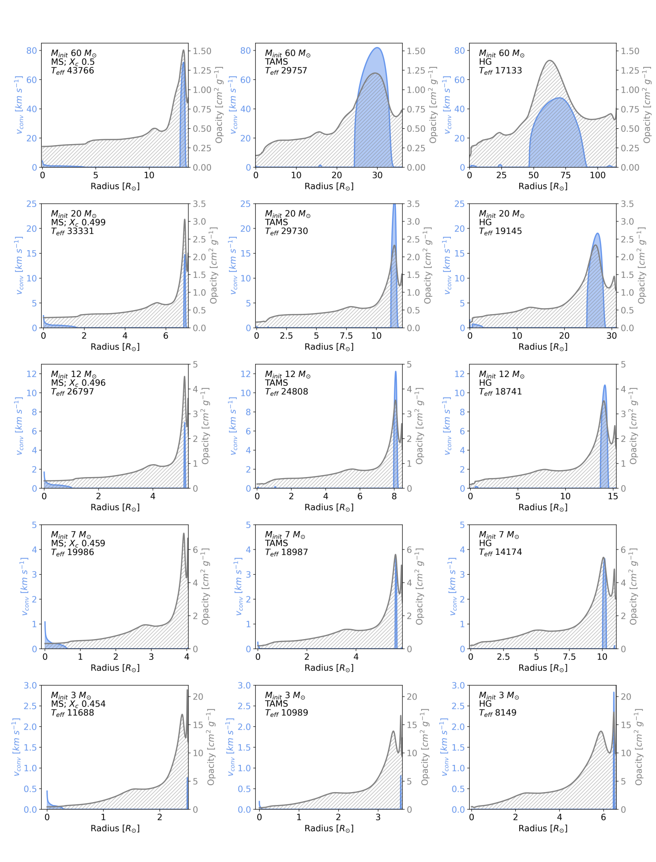
Figure 14: Profiles of opacity (grey) and convective velocity (blue) as a function of radius (full radius). The panels are the same as in Fig.12.

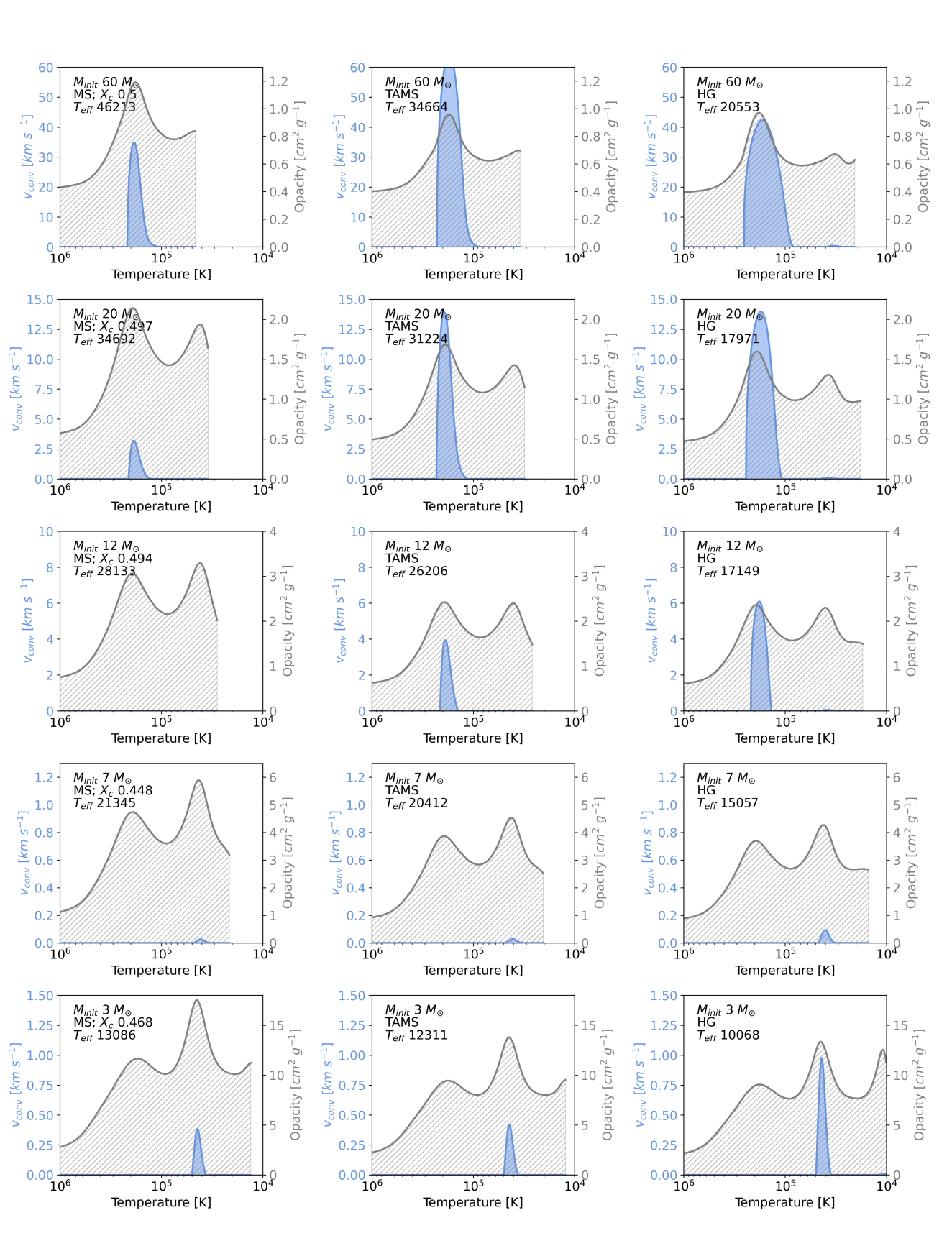
Figure 16: Profiles of opacity (grey) and convective velocity (blue) as a function of temperature. The panels are the same as in Fig.12 but for $Z$=0.006.

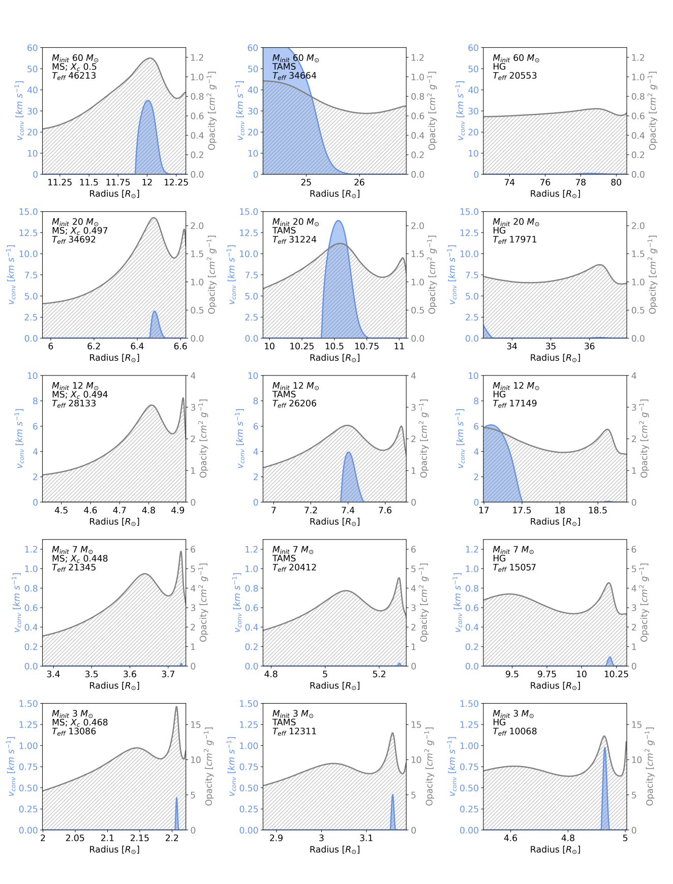
Figure 17: Profiles of opacity (grey) and convective velocity (blue) as a function of radius (zoomed into outer 10% of radius). The panels are the same as in Fig.12 but for $Z$=0.006.

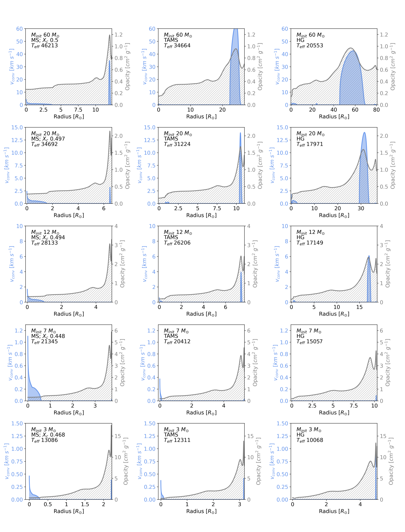
Figure 18: Profiles of opacity (grey) and convective velocity (blue) as a function of radius (full radius). The panels are the same as in Fig.12 but for $Z$=0.006.

Appendix D Propagation diagrams

Appendix E Detailed level-plots for FeCZ velocities and tunnelling of core-generated IGW

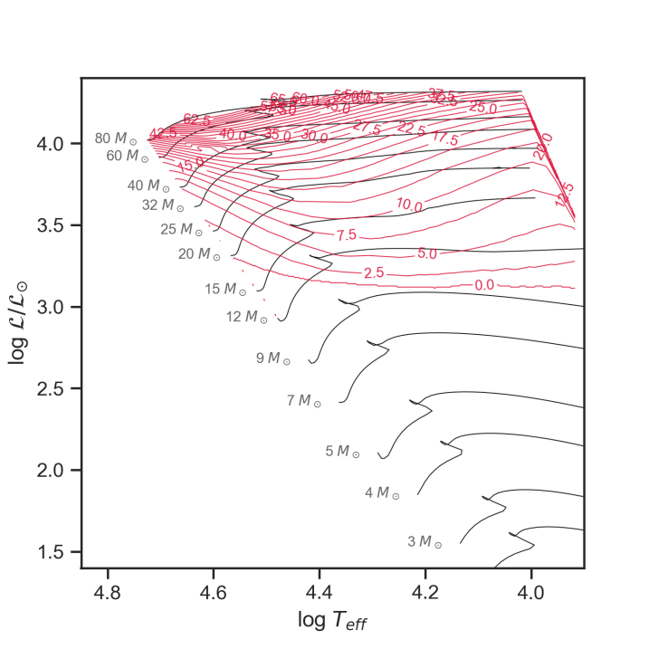
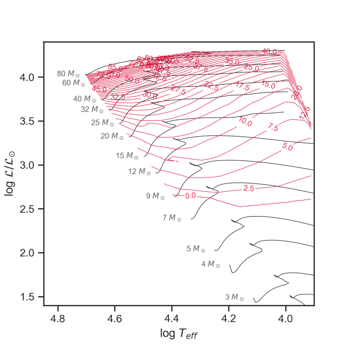
Figure 26: Level-plots of maximal convective velocities in FeCZ, labels are in km s^-1. Left panel – $Z$=0.006, right panel – $Z$=0.014.

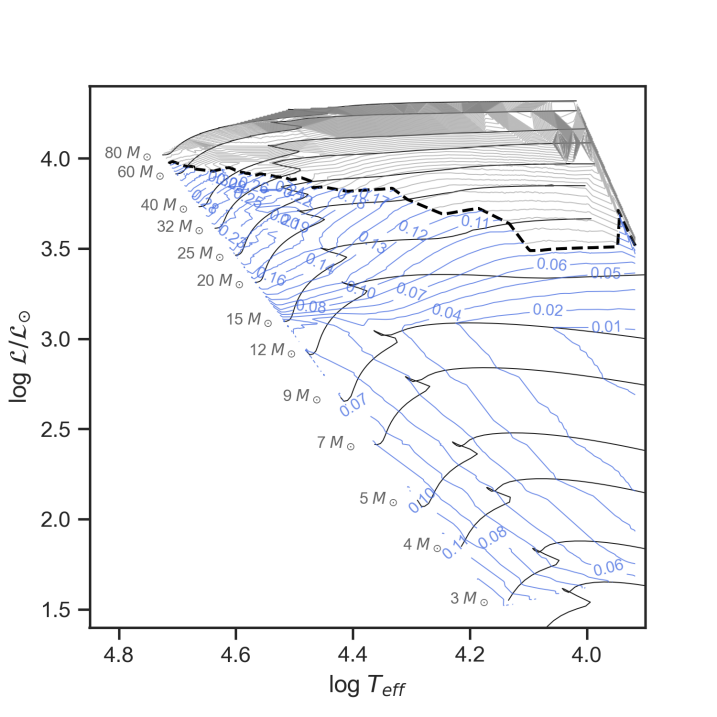
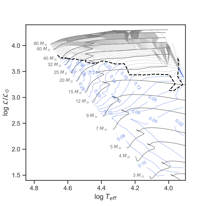
Figure 27: Level-plots tunnelling frequency, labels are in cycles per day. Left panel – $Z$=0.006, right panel – $Z$=0.014. The thick black line shows a cut-off forbidding tunnelling above it.