Catastrophic cooling in optically thin plasmas

Abstract

The solar corona is the prototypical example of a low density environment heated to high temperatures by external sources. The plasma cools radiatively, and because it is optically thin to this radiation, it becomes possible to model the density, velocity, and temperature structure of the system by modifying the MHD equations to include energy source terms that approximate the local heating and cooling rates. The solutions can be highly inhomogeneous and even multiphase because the well known linear instability associated with these source terms, thermal instability, leads to a catastrophic heating and cooling of the plasma in the nonlinear regime. Here we show that there is a separate, much simpler instance of catastrophic heating and cooling accompanying these source terms that can rival thermal instability in dynamical importance. The linear stability criterion is the isochoric one identified by Parker (1953), and we demonstrate that cooling functions derived from collisional ionization equilibrium are highly prone to violating this criterion. If catastrophic cooling instability can act locally in global simulations, then it is an alternative mechanism for forming condensations, and due to its nonequilibrium character, it may be relevant to explaining a host of phenomena associated with the production of cooler gas in hot, low density plasmas.

1 Introduction

Catastrophic cooling refers to a runaway radiative cooling of gas that proceeds so long as no balance with heating processes is reached. There will be an accompanying loss of pressure support as the thermal state of the gas departs further away from equilibrium, hence mechanical equilibrium will also be lost. A widely studied example of this occurs in the (multi-)million degree plasma within coronal loops (for recent reviews, see Antolin, 2020; Chen et al., 2020; Antolin & Froment, 2022). The descriptor ‘catastrophic cooling’ has been used to describe the bulk cooling observed in numerical simulations of pulse-heated loops (e.g. Reale & Landi, 2012; Cargill & Bradshaw, 2013), as well as to characterize the formation mechanism of both prominences and coronal rain (e.g. Antiochos et al., 1999; Schrijver, 2001; Aschwanden et al., 2001; Müller et al., 2004, 2005; Antolin et al., 2010; Peter et al., 2012). Most multi-dimensional simulation studies of coronal loops attribute coronal rain to be the outcome of local thermal instability (TI) (Fang et al., 2013, 2015; Moschou et al., 2015; Antolin et al., 2022; Daley-Yates et al., 2023; Donné & Keppens, 2024), a linear instability of non-adiabatic gas dynamics that was first elucidated by Field (1965).

The nonlinear regime of TI is itself a catastrophic cooling process, although one in which the density can rise by nearly the same factor that the temperature can drop. The way in which thermal equilibrium is regained in TI is commonly covered in textbooks and amounts to drawing an isobar on a pressure-density phase diagram connecting different points where heating can balance cooling (e.g. Shu, 1992). Only recently was the mechanism for restoring mechanical equilibrium shown to be damped oscillations mediated by sound waves (Waters & Proga, 2019, hereafter referred to as WP19); Waters & Proga (2023) confirmed this analytically and illustrated the limitations of the simple isobar analysis.

What might be regarded as evidence of coronal plasma ‘struggling’ to regain mechanical equilibrium upon cooling to a new thermal equilibrium temperature has emerged in the form of coincident observations of long-period intensity pulsations being in phase with periodic episodes of coronal rain (Auchère et al., 2018). The observed properties of these pulsations appear to lend support to the thermal nonequilibrium (TNE) model (Froment et al., 2015, 2017, 2018), which is an alternative scenario — specific to coronal loops — for forming condensations. It contrast to TI, it is a fully nonlinear process (Antiochos & Klimchuk, 1991; Antiochos et al., 1999, 2000; Karpen et al., 2005; Schlenker et al., 2021).

The TNE model distinguishes itself from a broader class of evaporation-condensation models (e.g. Priest & Smith, 1979; Poland & Mariska, 1986; Mok et al., 1990) through a heating deposition that is concentrated at the footpoints of a loop. While the mechanism leading to prominences in TNE involves a heating and cooling imbalance, Antiochos et al. (1999) comment that ‘this temperature collapse is physically due to a loss of equilibrium rather than to a thermal instability’. Moreover, Klimchuk (2019) asserts that TNE can lead to coronal rain production without TI. In simulations adopting the TNE heating prescription, however, coronal rain is still interpreted as being a result of TI (e.g. Fang et al., 2015; Antolin et al., 2022). Adding to the controversy, Fang et al. (2015) describe TNE as simply the nonlinear counterpart of TI, Donné & Keppens (2024) state that TNE is not a necessary condition for condensation formation in global loop simulations, and Antolin & Froment (2022) refer to the condensation process leading to either prominences or coronal rain as ‘TNE-TI cycles’.

Here we suggest that this contentious state of affairs has arisen because it has not been recognized that, separate from TI, there is an elementary linear theory solution to the equations of non-adiabatic MHD describing catastrophic heating and cooling. In §2, we present the linear theory of this instability and derive a criterion for it to overtake TI when both instabilities operate simultaneously. In §3, we demonstrate that commonly used radiative loss functions in solar physics, those representing collisional ionization equilibrium, are highly prone to violating the isochoric stability criterion that governs the eigenmode of this instability. In §4, we describe how these findings are relevant to resolving the above controversy. In the Appendix, we show that several authors have considered this solution but wrongly concluded that it could not act independently of TI.

2 Linear Theory

The net cooling function, $\mathcal{L}=\mathcal{L}(\rho,T)$, representing losses minus gains in units of $\rm{erg\,g^{-1}\,s^{-1}}$, enters the internal energy equation for non-adiabatic, ideal MHD as the volumetric source term $-\rho\mathcal{L}$:

$$\rho\frac{D\mathcal{E}}{Dt}=-p\mathbf{\nabla}\cdot\mbox{\boldmath$v$}-\rho\mathcal{L}-\mathbf{\nabla}\cdot\mbox{\boldmath$q$}.$$ (1)

Here, the variables $\rho$, $v$, and $p$ are the gas density, velocity, and pressure, respectively, $\mathcal{E}=c_{V}T$ is the gas internal energy, $q$ is the heat flux due to thermal conduction, and $D/Dt$ is the comoving frame derivative. In the rest frame of a homogeneous plasma (i.e. one with $\mathbf{\nabla}\cdot\mbox{\boldmath$v$}=0$ and $\mathbf{\nabla}\cdot\mbox{\boldmath$q$}=0$) with a constant specific heat capacity $c_{V}$, Eq. (1) becomes simply

$$c_{V}\frac{\partial T}{\partial t}=-\mathcal{L}.$$ (2)

The plasma reaches its thermal equilibrium temperature $T_{eq}$ when the heating and cooling rates balance ($\mathcal{L}=0$). In the linear theory of TI, Eq. (2) governs the background equilibrium state but the linearized version of Eq. (1) governs the evolution of perturbations. Because that equation involves $\delta\rho$, $\delta\mbox{\boldmath$v$}$, and $\delta p$, obtaining a dispersion relation requires linearizing the mass and momentum conservation equations also, which in turn requires linearizing the induction equation and the equation of state to obtain a closed set of equations. What has evidently been overlooked is that there is in fact an almost trivial solution requiring only the linearized version of Eq. (2): uniform temperature fluctuations $\delta T$, defined (for an ideal gas with $p=\rho kT/\bar{m}$) as perturbations satisfying $(\delta\rho,\delta\mbox{\boldmath$v$},\delta p,\delta\mbox{\boldmath$B$})=(0,\mbox{\boldmath$0$},\rho k\delta T/\bar{m},\mbox{\boldmath$0$})$, with $\delta T=\delta T(t)$ being spatially constant. This implies that no flows can develop as $\delta T$ is applied because both the gas density and pressure remain spatially constant.

2.1 Catastrophic heating/cooling instability

Letting $T=T_{eq}+\delta T$ and noting that $\mathcal{L}(T_{eq})=0$ by definition, we have for $\delta T\ll T_{eq}$,

$$\mathcal{L}(T_{eq}+\delta T)=\left(\frac{\partial\mathcal{L}}{\partial T}\right)_{\rho}\delta T.$$ (3)

Eq. (2) becomes

$$\frac{\partial\ln\delta T}{\partial t}=-\frac{1}{c_{V}}\left(\frac{\partial\mathcal{L}}{\partial T}\right)_{\rho},$$ (4)

which is an evolution equation for how $\delta T$ changes with time. The linear theory solution is found by taking $\left(\partial\mathcal{L}/\partial T\right)_{\rho}$ to be time-independent, giving

$$\delta T(t)=(\delta T)_{0}\exp\left[-\frac{1}{c_{V}}\left(\frac{\partial\mathcal{L}}{\partial T}\right)_{\rho}t\right],$$ (5)

where $(\delta T)_{0}$ is the initial temperature fluctuation above or below $T_{eq}$. Thus, the background equilibrium state is unstable to either catastrophic cooling, $(\delta T)_{0}<0$, or catastrophic heating, $(\delta T)_{0}>0$, whenever

$$\left(\frac{\partial\mathcal{L}}{\partial T}\right)_{\rho}<0.$$ (6)

This instability criterion is just the well known isochoric criterion for TI; see Field (1965).

Because the isochoric derivative is central to this result, we should emphasize that in Eq. (3), the $\rho$-subscript appears because we are assuming a temperature displacement along a vertical path on a $T$-vs-$\rho$ phase diagram. Alternatively, we can simply apply the Eulerian perturbation operator $\delta$ to Eq. (2), to give

$$\frac{\partial\delta T}{\partial t}=-\frac{\mathcal{\delta L}}{c_{V}}.$$ (7)

With $\mathcal{L}=\mathcal{L}(\rho,T)$, we have that

$$\mathcal{\delta L}=\left(\frac{\partial\mathcal{L}}{\partial T}\right)_{\rho}\delta T+\left(\frac{\partial\mathcal{L}}{\partial\rho}\right)_{T}\delta\rho.$$ (8)

Substituting Eq. (8) into Eq. (7) and considering solutions with $\delta\rho=0$ also gives Eq. (4).

Interestingly, Defouw (1970a) showed that Eq. (5) corresponds to the original solution obtained by Parker (1953) upon neglecting thermal conduction. As discussed in Appendix A, Defouw did not regard this solution as distinct from TI. In Appendix B, we explicitly verify that this solution does not correspond to the long wavelength limit of TI.

2.2 CC modes versus TI modes

Consider a plasma subjected to a random distribution of perturbation amplitudes and wavenumbers. As shown in §3, typical parameterizations of the heating rate that can balance the cooling rate of gas in collisional ionization equilibrium result in a wide parameter space where the plasma is simultaneously isobarically and isochorically unstable. Two questions then come to mind: (1) how do we distinguish between TI modes and the uniform temperature fluctuations leading to isochoric catastrophic cooling (referred to as simply CC modes in what follows)?; (2) given that the isobaric growth rate is often faster than the isochoric one, is it still possible for CC modes to dominate the evolution of the system?

If we confine our attention to a 1D local simulation of a homogeneous plasma that was initialized with a random set of perturbations, it is clear how to answer question (1). Let the domain extend from $-L$ to $L$ and have periodic boundary conditions. Then there is a Fourier series representation of the initial temperature profile given by

$$T(x)=\langle T(x)\rangle+\sum_{m=1}^{\infty}\left(a_{m}\cos k_{m}x+b_{m}\sin k_{m}x\right),$$ (9)

where $k_{m}=m\pi/L$ are individual wavenumbers, $a_{m}$ and $b_{m}$ are the Fourier coefficients (in this case, the perturbation amplitudes corresponding to $k_{m}$), and

$$\langle T(x)\rangle=\frac{1}{2L}\int_{-L}^{L}T(x)\,dx$$ (10)

is the average of the temperature profile. The CC mode has $\delta T<0$ and can be simply computed from the constant component as $\delta T=\langle T(x)\rangle-T_{eq}$. The rest of the Fourier decomposition will consist of a superposition of MHD waves and condensation modes susceptible to TI.

We answer question (2) in the affirmative by assuming that the perturbations to saturate first are those that become nonlinear first. We then define the timescale for reaching nonlinearity, $t_{non}$, through the equation

$$A\exp(\sigma t_{non})=\frac{1}{2},$$ (11)

where $\sigma$ is the instability growth rate. That is, we assume that exponential growth is halted once the amplitude of a perturbed quantity grows to half the background value of that quantity. For TI modes, we set $A=\delta\rho/\rho_{eq}$ (for background density $\rho_{eq}$) and take the growth rate to be that of the isobaric limit, namely $\sigma=-c_{p}^{-1}(\partial\mathcal{L}/\partial T)_{p}$ (see Defouw, 1970b), where $c_{p}$ is the specific heat at constant pressure. For CC modes, $A=\delta T/T_{eq}$ and by Eq. (4), $\sigma=-c_{V}^{-1}(\partial\mathcal{L}/\partial T)_{\rho}$. By Eq. (11) then,

$$t_{non}=\begin{dcases*}\frac{c_{p}}{|(\partial\mathcal{L}/\partial T)_{p}|}\ln\frac{2|\delta\rho|}{\rho_{eq}}&\text{ (TI modes)}\\ \frac{c_{V}}{|(\partial\mathcal{L}/\partial T)_{\rho}|}\ln\frac{2|\delta T|}{T_{eq}}&\text{ (CC modes).}\end{dcases*}$$ (12)

We expect a CC mode to dominate any particular TI mode whenever $(t_{non})_{CC}<(t_{non})_{TI}$, which corresponds to a lower bound on the magnitude of $\delta T$. Defining the ratio of specific heats $\gamma=c_{p}/c_{V}$ and the ratio of the isobaric and isochoric asymptotic growth rates,

$$R=\frac{1}{\gamma}\frac{(\partial\mathcal{L}/\partial T)_{p}}{(\partial\mathcal{L}/\partial T)_{\rho}},$$ (13)

which was shown by WP19 to be the basic parameter governing the various regimes of TI, this bound can be written

$$|\delta T|>\frac{1}{2}\left(\frac{2|\delta\rho|}{\rho_{eq}}\right)^{1/R}T_{eq}.$$ (14)

Returning to the above conceptual 1D simulation, there will be one $(a_{m},k_{m})$ or $(b_{m},k_{m})$ combination that corresponds to the TI mode with the shortest $t_{non}$. Denoting this mode by $\delta\rho_{max}$, we can express the above inequality as the following upper bound on the mean temperature:

$$\langle T(x)\rangle<\left[1-\frac{1}{2}\left(\frac{2|\delta\rho_{max}|}{\rho_{eq}}\right)^{1/R}\right]T_{eq}.$$ (15)

To use this bound, note that WP19 showed that $R\geq 1$ when a plasma is thermally unstable by both the isochoric and isobaric criterion—unless the isentropic instability criterion is also satisfied, implying the overstability of acoustic modes, in which case $1/\gamma<R<1$ (see their Appendix B). Because $R$ is the ratio of the maximum isobaric and isochoric growth rates, the CC mode grows faster than all condensation modes in plasmas with $0<R<1$. A typical case might be $R\approx 1$ and $|\delta\rho_{max}|/\rho_{eq}=0.1$, putting the cutoff at $0.9\,T_{eq}$. Below this temperature, we would expect the CC mode to control the thermal state of the gas, meaning it can overcome the runaway heating taking place in the under-dense portion of all TI modes, resulting in the catastrophic cooling of the entire plasma — a ‘single-phase’ rather than ‘two-phase’ outcome.

In a forthcoming paper (Stricklan & Waters, in prep.), we will present MHD simulations showing that condition (15) indeed determines whether TI modes or CC modes control the outcome of an isochorically unstable homogenous plasma containing random perturbations.

3 Isochoric instability

As Balbus (1995) commented, the isochoric instability criterion as given by condition (6) is much more difficult to satisfy compared to the isobaric one, $(\partial\mathcal{L}/\partial T)_{p}<0$, and this has proved true for cooling functions derived from photoionization equilibrium (see e.g. Hess et al., 1997; Chakravorty et al., 2009; Dannen et al., 2019). However, it turns out to be easily satisfied for cooling functions based on collisional ionization equilibrium (CIE), as first noted by Goldsmith (1971) for the CIE-based radiative loss function of Cox & Tucker (1969).

WP19 derived a simple graphical criterion for judging if there are regions on the equilibrium curve with $(\partial\mathcal{L}/\partial T)_{\rho}<0$: the slope of those regions when plotted on the $\log T$ vs. $\log n$ plane must be positive. This result follows immediately from the identity

$$\left(\frac{\partial T}{\partial\rho}\right)_{\mathcal{L}}=-\frac{(\partial\mathcal{L}/\partial\rho)_{T}}{(\partial\mathcal{L}/\partial T)_{\rho}}.$$ (16)

Multiplying both sides by $\rho/T$ (and introducing a mean particle mass $\bar{m}=\rho/n$ to exchange $\rho$ for the number density $n$) gives

$$\left(\frac{\partial\log T}{\partial\log n}\right)_{\mathcal{L}}=-\frac{\rho}{T}\frac{(\partial\mathcal{L}/\partial\rho)_{T}}{(\partial\mathcal{L}/\partial T)_{\rho}}.$$ (17)

The logarithmic derivative is just the slope of the equilibrium curve (the contour where $\mathcal{L}$ vanishes), and its sign depends on the isochoric temperature derivative in the denominator on the right hand side. Thus, this slope is positive whenever $(\partial\mathcal{L}/\partial T)_{\rho}<0$ provided $(\partial\mathcal{L}/\partial\rho)_{T}>0$, which is the statement that the plasma should cool when the density is increased at a fixed temperature — a property that is difficult to not satisfy.

WP19 also showed that if $(\partial\mathcal{L}/\partial\rho)_{T}>0$ and $(\partial\mathcal{L}/\partial T)_{\rho}<0$, it must be the case that the isobaric instability criterion, $(\partial\mathcal{L}/\partial T)_{p}<0$, is also satisfied. We used this property in §2.2 to constrain the value of $R$ appearing in condition Eq. (15). The reason we refer to ‘TI modes’ rather than just condensation modes is due to yet another property of TI: when the plasma is both isochorically and isobarically unstable, all three varieties of condensation modes (what WP19 called the entropy mode and the fast and slow isochoric modes) can exist for $R<1/3$. For $R>1/3$, just one condensation mode remains (the fast isochoric one) and its stability, like the CC mode, is set by the sign of the derivative $(\partial\mathcal{L}/\partial T)_{\rho}$. The isobaric derivative $(\partial\mathcal{L}/\partial T)_{p}$ is instead tied to an overstable acoustic wave.

3.1 CIE-based cooling functions

For CIE-based cooling functions, the property $(\partial\mathcal{L}/\partial\rho)_{T}>0$ should probably be regarded as a physical constraint on the density-dependence of the coronal heating rate. A widely used form of the net cooling source term from Eq. (1) in solar corona modeling is

$$\rho\mathcal{L}=n^{2}\Lambda(T)-Cp^{a}T^{b},$$ (18)

where $\Lambda(T)$ is the radiative loss function and $C$ is a constant. This specification of the heating rate dependence follows Dahlburg & Mariska (1988), who quoted values of $a$ and $b$ appropriate for the various heating mechanism dependencies identified by Rosner et al. (1978). Solving Eq. (18) for $\mathcal{L}$ gives

$$\mathcal{L}=\frac{\rho}{\bar{m}^{2}}\Lambda(T)-C_{H}\left(\frac{\rho}{\rho_{eq}}\right)^{a-1}\left(\frac{T}{T_{eq}}\right)^{a+b},$$ (19)

where we have eliminated $n$ and $p$ in favor of $\rho$ and defined a new heating constant that is given by $C_{H}=(\rho_{eq}/\bar{m}^{2})\Lambda(T_{eq})$, chosen according to the desired starting location $(\rho_{eq},T_{eq})$ along the equilibrium curve. Taking the derivative with respect to $\rho$ at fixed $T$ gives

$$\left(\frac{\partial\mathcal{L}}{\partial\rho}\right)_{T}=\frac{1}{\bar{m}^{2}}\Lambda(T)+(1-a)\frac{C_{H}}{\rho_{eq}}\left(\frac{\rho}{\rho_{eq}}\right)^{a-2}\left(\frac{T}{T_{eq}}\right)^{a+b},$$ (20)

showing that this derivative will always be positive provided $a\leq 1$. The only heating mechanism discussed by Rosner et al. (1978) that has $a>1$ is Alfven wave damping (with $a=7/6$), but that dependence may still keep $(\partial\mathcal{L}/\partial\rho)_{T}>0$. In any case, the one-to-one correspondence between positive slopes and isochoric instability certainly holds for $a\leq 1$.

In Fig. 1, we plot the equilibrium curve for the most common choice of heating parameters in numerical studies: $a=b=0$, corresponding to a constant volumetric heating rate (see Eq. (18)). The portion of this curve with $3\times 10^{5}\rm{K}<T<3\times 10^{6}\rm{K}$ has a positive slope and thus satisfies the isochoric instability criterion. The colormap makes this intuitively obvious: on negative sloping portions of the curve, a vertical displacement below equilibrium puts the gas into a (red) net heating region, where it will return to equilibrium. But on positive sloping portions, such as the one marked by an arrow, gas is unstable because it enters a (blue) net cooling region.

That the overall occurrence of isochoric instability is not sensitive to the choice of $\Lambda(T)$ or the heating parameters is easily demonstrated. In Fig. 1, we used a standard radiative loss function, one based on a piecewise powerlaw fit of the tabular function given in Table 2 of Schure et al. (2009), which was calculated using the SPEX package (Kaastra & Mewe, 2000). Hermans & Keppens (2021b) compared this $\Lambda(T)$ with several other popular functions based on CIE (including Klimchuk & Cargill (2001); Colgan et al. (2008)); all curves showed a non-monotonic rise of the cooling rate to a peak around $10^{5}\,\rm{K}$, followed by non-monotonic fall as temperature increases. In other words, there are several temperature ranges for which $d\Lambda(T)/dT<0$. From Eq. (19) with $a+b=0$, there is a very simple correspondence between the slope of $\Lambda(T)$ itself and the value of the isochoric derivative, namely

$$\left(\frac{\partial\mathcal{L}}{\partial T}\right)_{\rho}=\frac{\rho}{\bar{m}^{2}}\frac{d\Lambda(T)}{dT}\text{\hskip 25.0pt($a+b=0$)}.$$ (21)

Thus, all temperatures for which $\Lambda(T)$ decreases with $T$ are isochorically unstable; this property of radiative loss functions has long been recognized (see Gehrels & Williams, 1993, and references therein).

Intuitively, when $d\Lambda(T)/dT<0$ and the heating rate is constant, gas at fixed density that started to cool slightly will keep cooling at a higher rate. When $a+b\neq 0$, this simple correspondence between isochoric instability and the shape of the radiative loss function no longer holds, but that with positive slopes of the equilibrium curve on the $(\log T,\log n)$-plane still does.

For arbitrary $a$ and $b$,

$$\left(\frac{\partial\mathcal{L}}{\partial T}\right)_{\rho}=\frac{\rho}{\bar{m}^{2}}\frac{d\Lambda(T)}{dT}-(a+b)\frac{C_{H}}{T_{eq}}\left(\frac{\rho}{\rho_{eq}}\right)^{a-1}\left(\frac{T}{T_{eq}}\right)^{a+b-1},$$ (22)

revealing that the heating term has a stabilizing contribution to the isochoric derivative when $a+b<0$. Referring again to Rosner et al. (1978), only one of the identified dissipation mechanisms satisfies this: the conductive damping of Alfven modes ($a=1/2$, $b=-1$). Hence, the occurrence of isochoric instability appears to be the norm for CIE-based cooling functions.

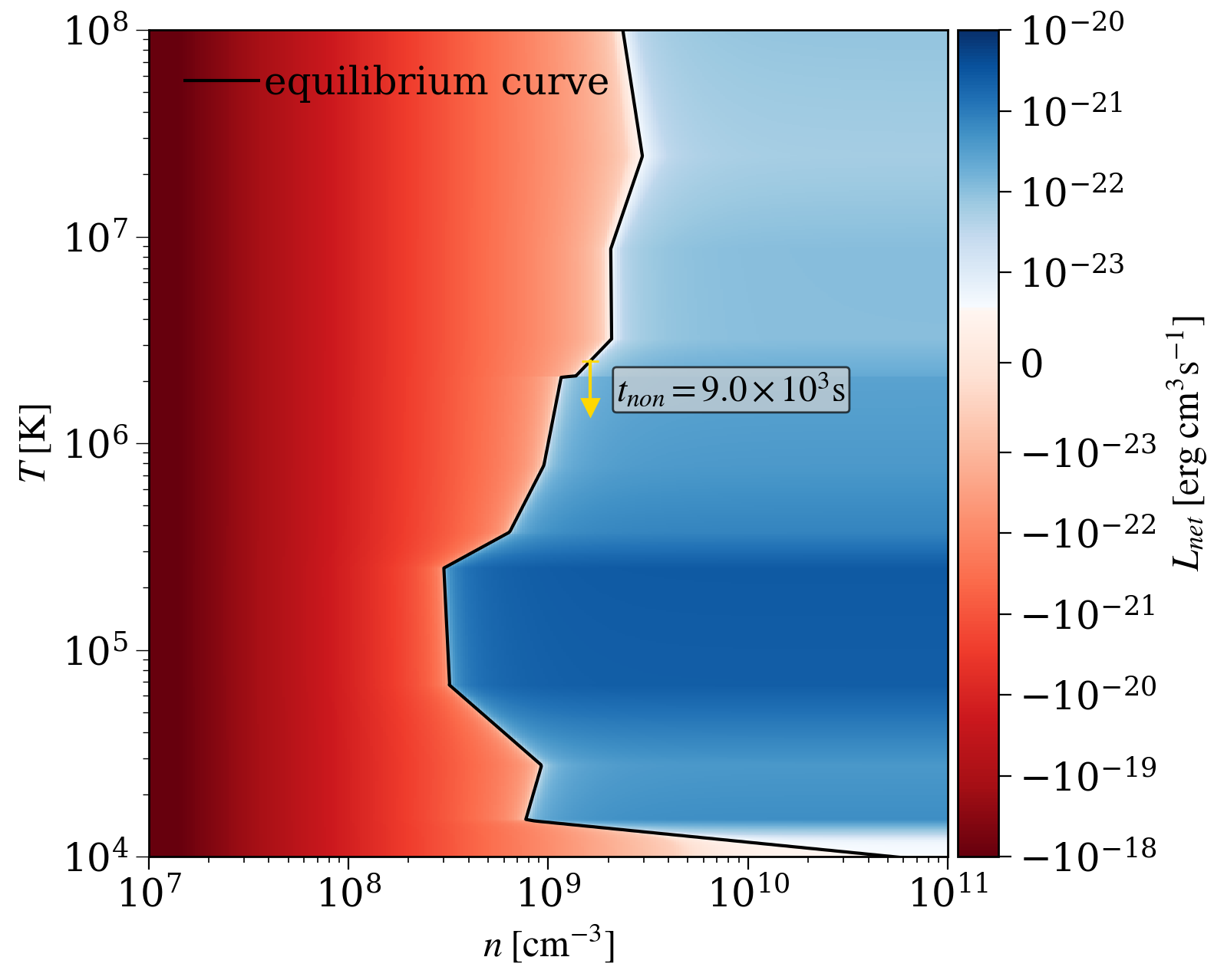
Figure 1: Temperature-density phase diagram for a plasma in CIE subject to a constant volumetric heating rate. The colormap shows $L_{\rm{net}}=(\bar{m}/n)\mathcal{L}$ calculated using a piecewise powerlaw fit to the SPEX radiative loss function of Schure et al. (2009). In blue (red) regions, $\mathcal{L}>0$ ($\mathcal{L}<0$), indicating net cooling (heating). Overplotted is the contour $\mathcal{L}=0$; all positive-sloping segments of this equilibrium curve are both isobarically and isochorically unstable and plasma there will undergo catastrophic cooling instability in addition to TI. The arrow points along an isochoric path and depicts the characteristic timescale for the catastrophic cooling mode to become nonlinear starting from an amplitude $\delta T=-10^{3}{\rm K}$ ($|\delta T|/T_{eq}=4\times 10^{-4}$). The additional time to reach the stable equilibrium location at $T\approx 1.5\times 10^{4}{\rm K}$ is $\Delta t\approx 0.1\,t_{non}$.

While we are not the first to report on the occurrence of isochoric TI in CIE-based cooling functions (e.g. Xia et al., 2011; Moschou et al., 2015; Jer$\mathbf{c}$ić et al., 2024), we know of only one example of a phase diagram showing the equilibrium curve: that given in the Appendix of Hermans & Keppens (2021b), which does not however have a colormap of the net cooling function as in our Fig. 1. Returning to this figure, it is clear that starting from temperatures above or below the equilibrium curve, a static, homogeneous plasma will not isochorically approach $T_{eq}$ unless $T_{eq}$ lies on a stable location. The question how plasma can occupy unstable locations in the first place is a very good one and deserves comment. In local simulations, the only way is to set initial conditions with $T=T_{eq}$. In global simulations, the velocity field can allow flows to settle into unstable parameter space slightly off the equilibrium curve.

For example, after Dannen et al. (2020) uncovered TI operating in 1D Parker-like wind solutions (in calculations based on photoionization equilibrium), Waters et al. (2021) obtained steady state versions of these solutions upon reducing the amplitude of perturbations associated with the interpolation of the tabular source term. These studies demonstrated that condensation modes have no chance of growing if gradients in the velocity field can stretch the modes before TI can amplify them. General flow fields therefore do not necessarily ‘avoid’ unstable parameter space unless the cooling timescale is much shorter than the dynamical timescale.

4 Summary and conclusions

We have presented the following results:

• Catastrophic cooling instability is a separate linear instability than TI that obeys the simple (and wavenumber-independent) dispersion relation $\sigma=-(1/c_{V})(\partial\mathcal{L}/\partial T)_{\rho}$. Its associated eigenvector, denoted the CC mode, is simply the difference between the mean plasma temperature and the initial equilibrium temperature.

• The CC mode can dominate all thermally unstable condensation modes in the system when the mean plasma temperature obeys the upper bound given in condition (15), in which case the outcome of a local simulation should be a single cold phase rather than a ‘two-phase’ medium.

• Cooling functions derived from collisionial ionization equilibrium are prone to violating the isochoric instability criterion that governs CC modes.

As for the second result, it is unclear what the outcome will be when the CC mode is dominated by only a few fast growing condensation modes. Such modes would have the shortest wavelengths allowed by linear theory, i.e. $\lambda>\lambda_{F}$, where $\lambda_{F}$ is the Field length (Begelman et al., 1983), so there may not be enough hot plasma produced in the underdense portions of these modes to overcome the bulk cooling by the CC mode. One would then expect a two-phase medium that is mostly cold gas with embedded pockets of hot gas (the remnants of the short wavelength condensation modes). If we then extrapolate this expectation when considering a local region within a global simulation, we arrive at a mechanism for producing larger condensations than are possible with isobaric TI modes.

Alternatively, in global simulations, the CC mode may only have enough time to partially cool a small region of background gas (much smaller than the density scale height $\lambda_{\rho}=\rho/|\nabla\rho|$ of a stratified atmosphere, for example) before the dynamics associated with either the surrounding plasma or the saturation of TI disrupt its growth. This latter outcome may account for what Mikić et al. (2013) labeled ‘complete’ versus ‘incomplete’ condensations in a parameter study of 1D coronal loop models (see also Froment et al., 2018).

Either of the above outcomes is expected to lead to oscillatory dynamics akin to the nonisobaric regime of TI (see WP19, ). The distinguishing property of CC modes is the accompanying loss of pressure support, so as the perturbation becomes nonlinear, strong flows can develop as mechanical equilibrium becomes lost during the evolution away from thermal equilibrium. This nonisobaric dynamics may offer a natural explanation for the observed long intensity pulsations accompanying some types of coronal rain (Antolin & Froment, 2022). Moreover, the overall tendency for the evolution to runaway from equilibrium leads us to suggest that the growth of CC modes is the mechanism underlying condensation formation in the TNE model discussed in §1.

Our analysis has centered on catastrophic cooling because our interests are in understanding coronal rain. We could have instead focused on an instance of catastrophic heating by reversing the green arrow in Fig. 1 and considering a $\delta T>0$ perturbation (i.e. a CH mode) of partially heated coronal plasma located on the equilibrium curve at $T\approx 3\times 10^{5}\,\rm{K}$. Since there is no stable equilibrium in this direction, the plasma temperature would rise to values in excess of $10^{6}\,\rm{K}$ where conductive losses could supply a balance. It would of course be remarkable if this local instability — based on a single, simple ordinary differential equation — is relevant to the solution of the famous coronal heating problem (e.g. Klimchuk, 2006). The important property to consider is its monolithic character: when this instability operates in a region of constant density, it will uniformly heat or cool that entire region. In contrast, condensation growth through TI involves a local force, i.e. it is the pressure gradient between the overdense and underdense gas that drives perturbation growth, hence TI can only operate on the scales of individual modes. If catastrophic heating instability was to play any role at all, it would probably be in tipping the balance in favor of overall heating by continually amplifying the CH modes supplied by magnetic dissipation processes.

Appendix A The early literature on TI

Several authors concluded early on that Parker’s demonstration of an instability arising from the heat equation alone (see Parker, 1953) could not actually manifest when solving the coupled equations of non-adiabatic, compressible MHD. For example, referring to Parker’s study as well as Athay & Thomas (1956), Weymann (1960) states ‘one ought perhaps to consider the stability criterion of Athay & Thomas and of Parker, as applying to the case of incompressible fluids, since arbitrary disturbances will affect the density as well as the temperature of the medium…’. Upon viewing an arbitrary disturbance as consisting of a constant displacement above or below $T_{eq}$ in addition to a superposition of acoustic or condensation modes (see §2.2), it becomes clear that TI governs only the latter modes, while the constant displacement $\delta T=\langle T(x)\rangle-T_{eq}$ is the mode of a separate instability altogether. The instability acts to exponentially amplify the magnitude of $\delta T$ — the departure of the mean temperature away from equilibrium — and thus catastrophic cooling/heating instability is an appropriate name.

Equations (1), (2), and (3) of Defouw (1970a)’s important study showing that a thermally unstable stratified atmosphere is also convectively unstable are precisely Eq. (2), Eq. (4), and Eq. (6) here. He discounts this solution by stating the following:

Weymann (1960) pointed out that the condition (3) for thermal instability applies only to isochoric perturbations. But density perturbations are to be expected, owing to the strong tendency of a fluid to remain in pressure equilibrium. A work term must therefore be added to equation (1), and the density dependence of the heat-loss function must be taken into account.

This is a true statement and leads one to the dispersion relation for TI, but it is not a valid reason to ignore the instability described by his starting equations.

Appendix B The long wavelength limit of TI

Our claim has been that the CC mode does not correspond to the asymptotic limit of any particular TI mode (i.e. of a condensation mode or an overstable acoustic wave). Intuitively, TI modes are ‘centered about equilibrium’, whereas the CC mode is a finite displacement above or below $T_{eq}$. Formally, we can eliminate consideration of the $k=0$ asymptotic limit of overstable modes by noting that their growth rates in this limit are always proportional to either $k$ or $k^{2}$ (see Figure 2 from WP19, ). Only the fast isochoric condensation mode has the same growth rate as the CC mode in this limit. We therefore just need to examine the analytic solution for condensation modes, which can be written as (see Waters & Proga, 2023)

$$\begin{split}\rho(\mbox{\boldmath$x$},t)&=\rho_{0}+A\rho_{0}e^{\sigma t}\cos(\mbox{\boldmath$k$}\cdot{\mbox{\boldmath$x$}})\\ v(\mbox{\boldmath$x$},t)&=v_{0}-Av_{c}e^{\sigma t}\sin(\mbox{\boldmath$k$}\cdot{\mbox{\boldmath$x$}})\\ p(\mbox{\boldmath$x$},t)&=p_{0}-A\rho_{0}v_{c}^{2}e^{\sigma t}\cos(\mbox{\boldmath$k$}\cdot{\mbox{\boldmath$x$}}),\end{split}$$ (B1)

where $\rho_{0}$, $v_{0}$, and $p_{0}$ are the density, velocity, and pressure of the uniform background flow, $A$ is the perturbation amplitude, and $v_{c}\equiv\sigma/k$ (for wavenumber $k=|\mbox{\boldmath$k$}|$) is the solution to the following cubic dispersion relation:

$$v_{c}=-\frac{k^{-1}}{c_{V}}\left(\frac{\partial\mathcal{L}}{\partial T}\right)_{\rho}\frac{R+(v_{c}/c_{s,0})^{2}}{1+(v_{c}/c_{s,0})^{2}}.$$ (B2)

Here, $c_{s,0}=\sqrt{\gamma p_{0}/\rho_{0}}$ is the sound speed in the background flow.

The long wavelength limit of TI has been associated with isochoric instability in the early literature because upon substituting back in for $\sigma=kv_{c}$ and taking the limit $k\rightarrow 0$, one obtains the isochoric growth rate $\sigma=c_{V}^{-1}(\partial\mathcal{L}/\partial T)_{\rho}$. However, as explained by WP19 and Waters & Proga (2023), the long wavelength limit should instead be thought of as the highly nonisobaric regime of TI, characterized by condensation velocities $v_{c}$ exceeding the speed of sound. Indeed, taking the limit $v_{c}\gg c_{s,0}$ in Eq. (B2) more directly gives back $\sigma=c_{V}^{-1}(\partial\mathcal{L}/\partial T)_{\rho}$. The isobaric regime of TI, on the other hand, has $v_{c}\ll c_{s,0}$, and Eq. (B2) gives back $\sigma=c_{p}^{-1}(\partial\mathcal{L}/\partial T)_{p}$ instead. In both limits, therefore, the condensation velocity scales as $v_{c}\propto k^{-1}$. Referring to the analytic solution above, the only way to recover the CC mode is to demand $A\propto k^{2}$ so that both $A$ and $Av_{c}$ vanish as $k\rightarrow 0$, while $Av_{c}^{2}$ can remain finite. Since $A$ is just an arbitrary amplitude, we must conclude that the CC mode is not contained in the asymptotic limit of TI.

References

- Antiochos & Klimchuk (1991) Antiochos, S. K., & Klimchuk, J. A. 1991, ApJ, 378, 372, doi: 10.1086/170437
- Antiochos et al. (2000) Antiochos, S. K., MacNeice, P. J., & Spicer, D. S. 2000, ApJ, 536, 494, doi: 10.1086/308922
- Antiochos et al. (1999) Antiochos, S. K., MacNeice, P. J., Spicer, D. S., & Klimchuk, J. A. 1999, ApJ, 512, 985, doi: 10.1086/306804
- Antolin (2020) Antolin, P. 2020, Plasma Physics and Controlled Fusion, 62, 014016, doi: 10.1088/1361-6587/ab5406
- Antolin & Froment (2022) Antolin, P., & Froment, C. 2022, Frontiers in Astronomy and Space Sciences, 9, 820116, doi: 10.3389/fspas.2022.820116
- Antolin et al. (2022) Antolin, P., Martínez-Sykora, J., & Şahin, S. 2022, ApJ, 926, L29, doi: 10.3847/2041-8213/ac51dd
- Antolin et al. (2010) Antolin, P., Shibata, K., & Vissers, G. 2010, ApJ, 716, 154, doi: 10.1088/0004-637X/716/1/154
- Aschwanden et al. (2001) Aschwanden, M. J., Poland, A. I., & Rabin, D. M. 2001, ARA&A, 39, 175, doi: 10.1146/annurev.astro.39.1.175
- Athay & Thomas (1956) Athay, R. G., & Thomas, R. N. 1956, ApJ, 123, 299, doi: 10.1086/146162
- Auchère et al. (2018) Auchère, F., Froment, C., Soubrié, E., et al. 2018, ApJ, 853, 176, doi: 10.3847/1538-4357/aaa5a3
- Balbus (1995) Balbus, S. A. 1995, in Astronomical Society of the Pacific Conference Series, Vol. 80, The Physics of the Interstellar Medium and Intergalactic Medium, ed. A. Ferrara, C. F. McKee, C. Heiles, & P. R. Shapiro, 328
- Begelman et al. (1983) Begelman, M. C., McKee, C. F., & Shields, G. A. 1983, ApJ, 271, 70, doi: 10.1086/161178
- Cargill & Bradshaw (2013) Cargill, P. J., & Bradshaw, S. J. 2013, ApJ, 772, 40, doi: 10.1088/0004-637X/772/1/40
- Chakravorty et al. (2009) Chakravorty, S., Kembhavi, A. K., Elvis, M., & Ferland, G. 2009, MNRAS, 393, 83, doi: 10.1111/j.1365-2966.2008.14249.x
- Chen et al. (2020) Chen, P.-F., Xu, A.-A., & Ding, M.-D. 2020, Research in Astronomy and Astrophysics, 20, 166, doi: 10.1088/1674-4527/20/10/166
- Colgan et al. (2008) Colgan, J., Abdallah, J., J., Sherrill, M. E., et al. 2008, ApJ, 689, 585, doi: 10.1086/592561
- Cox & Tucker (1969) Cox, D. P., & Tucker, W. H. 1969, ApJ, 157, 1157, doi: 10.1086/150144
- Dahlburg & Mariska (1988) Dahlburg, R. B., & Mariska, J. T. 1988, Sol. Phys., 117, 51, doi: 10.1007/BF00148571
- Daley-Yates et al. (2023) Daley-Yates, S., Jardine, M. M., & Johnston, C. D. 2023, MNRAS, 526, 1646, doi: 10.1093/mnras/stad2752
- Dannen et al. (2019) Dannen, R. C., Proga, D., Kallman, T. R., & Waters, T. 2019, ApJ, 882, 99, doi: 10.3847/1538-4357/ab340b
- Dannen et al. (2020) Dannen, R. C., Proga, D., Waters, T., & Dyda, S. 2020, ApJ, 893, L34, doi: 10.3847/2041-8213/ab87a5
- Defouw (1970a) Defouw, R. J. 1970a, ApJ, 160, 659, doi: 10.1086/150460
- Defouw (1970b) —. 1970b, ApJ, 161, 55, doi: 10.1086/150512
- Donné & Keppens (2024) Donné, D., & Keppens, R. 2024, ApJ, 971, 90, doi: 10.3847/1538-4357/ad50a3
- Fang et al. (2013) Fang, X., Xia, C., & Keppens, R. 2013, ApJ, 771, L29, doi: 10.1088/2041-8205/771/2/L29
- Fang et al. (2015) Fang, X., Xia, C., Keppens, R., & Van Doorsselaere, T. 2015, ApJ, 807, 142, doi: 10.1088/0004-637X/807/2/142
- Field (1965) Field, G. B. 1965, ApJ, 142, 531, doi: 10.1086/148317
- Froment et al. (2017) Froment, C., Auchère, F., Aulanier, G., et al. 2017, ApJ, 835, 272, doi: 10.3847/1538-4357/835/2/272
- Froment et al. (2015) Froment, C., Auchère, F., Bocchialini, K., et al. 2015, ApJ, 807, 158, doi: 10.1088/0004-637X/807/2/158
- Froment et al. (2018) Froment, C., Auchère, F., Mikić, Z., et al. 2018, ApJ, 855, 52, doi: 10.3847/1538-4357/aaaf1d
- Gehrels & Williams (1993) Gehrels, N., & Williams, E. D. 1993, ApJ, 418, L25, doi: 10.1086/187107
- Goldsmith (1971) Goldsmith, D. W. 1971, Sol. Phys., 19, 86, doi: 10.1007/BF00148826
- Hermans & Keppens (2021a) Hermans, J., & Keppens, R. 2021a, in 47th EPS Conference on Plasma Physics
- Hermans & Keppens (2021b) Hermans, J., & Keppens, R. 2021b, A&A, 655, A36, doi: 10.1051/0004-6361/202140665
- Hess et al. (1997) Hess, C. J., Kahn, S. M., & Paerels, F. B. S. 1997, ApJ, 478, 94, doi: 10.1086/303783
- Jerić et al. (2024) Jerić, V., Jenkins, J. M., & Keppens, R. 2024, A&A, 688, A145, doi: 10.1051/0004-6361/202348442
- Kaastra & Mewe (2000) Kaastra, J. S., & Mewe, R. 2000, in Atomic Data Needs for X-ray Astronomy, ed. M. A. Bautista, T. R. Kallman, & A. K. Pradhan, 161
- Karpen et al. (2005) Karpen, J. T., Tanner, S. E. M., Antiochos, S. K., & DeVore, C. R. 2005, ApJ, 635, 1319, doi: 10.1086/497531
- Klimchuk (2006) Klimchuk, J. A. 2006, Sol. Phys., 234, 41, doi: 10.1007/s11207-006-0055-z
- Klimchuk (2019) —. 2019, Sol. Phys., 294, 173, doi: 10.1007/s11207-019-1562-z
- Klimchuk & Cargill (2001) Klimchuk, J. A., & Cargill, P. J. 2001, ApJ, 553, 440, doi: 10.1086/320666
- Mikić et al. (2013) Mikić, Z., Lionello, R., Mok, Y., Linker, J. A., & Winebarger, A. R. 2013, ApJ, 773, 94, doi: 10.1088/0004-637X/773/2/94
- Mok et al. (1990) Mok, Y., Drake, J. F., Schnack, D. D., & van Hoven, G. 1990, ApJ, 359, 228, doi: 10.1086/169053
- Moschou et al. (2015) Moschou, S. P., Keppens, R., Xia, C., & Fang, X. 2015, Advances in Space Research, 56, 2738, doi: 10.1016/j.asr.2015.05.008
- Müller et al. (2005) Müller, D. A. N., De Groof, A., Hansteen, V. H., & Peter, H. 2005, A&A, 436, 1067, doi: 10.1051/0004-6361:20042141
- Müller et al. (2004) Müller, D. A. N., Peter, H., & Hansteen, V. H. 2004, A&A, 424, 289, doi: 10.1051/0004-6361:20040403
- Parker (1953) Parker, E. N. 1953, ApJ, 117, 431, doi: 10.1086/145707
- Peter et al. (2012) Peter, H., Bingert, S., & Kamio, S. 2012, A&A, 537, A152, doi: 10.1051/0004-6361/201117889
- Poland & Mariska (1986) Poland, A. I., & Mariska, J. T. 1986, Sol. Phys., 104, 303, doi: 10.1007/BF00159083
- Priest & Smith (1979) Priest, E. R., & Smith, E. A. 1979, Sol. Phys., 64, 267, doi: 10.1007/BF00151439
- Reale & Landi (2012) Reale, F., & Landi, E. 2012, A&A, 543, A90, doi: 10.1051/0004-6361/201219280
- Rosner et al. (1978) Rosner, R., Tucker, W. H., & Vaiana, G. S. 1978, ApJ, 220, 643, doi: 10.1086/155949
- Schlenker et al. (2021) Schlenker, M. J., Antiochos, S. K., MacNeice, P. J., & Mason, E. I. 2021, ApJ, 916, 115, doi: 10.3847/1538-4357/ac069d
- Schrijver (2001) Schrijver, C. J. 2001, Sol. Phys., 198, 325, doi: 10.1023/A:1005211925515
- Schure et al. (2009) Schure, K. M., Kosenko, D., Kaastra, J. S., Keppens, R., & Vink, J. 2009, A&A, 508, 751, doi: 10.1051/0004-6361/200912495
- Shu (1992) Shu, F. H. 1992, Physics of Astrophysics, Vol. II
- Waters & Proga (2019) Waters, T., & Proga, D. 2019, ApJ, 875, 158, doi: 10.3847/1538-4357/ab10e1
- Waters & Proga (2023) —. 2023, Frontiers in Astronomy and Space Sciences, 10, 1198135, doi: 10.3389/fspas.2023.1198135
- Waters et al. (2021) Waters, T., Proga, D., & Dannen, R. 2021, ApJ, 914, 62, doi: 10.3847/1538-4357/abfbe6
- Weymann (1960) Weymann, R. 1960, ApJ, 132, 452, doi: 10.1086/146942
- Xia et al. (2011) Xia, C., Chen, P. F., Keppens, R., & van Marle, A. J. 2011, ApJ, 737, 27, doi: 10.1088/0004-637X/737/1/27