About the first eigenvector of the simple random walk
killed upon exiting a large bounded domain

Abstract

In this article, we study a discrete version of a Dirichlet problem in an open bounded set $D\subset\mathbb{R}^{d}$, in dimension $d\geq 2$. More precisely, we consider the simple random walk on $\mathbb{Z}^{d}$, $d\geq 2$, killed upon exiting the large (bounded) domain $D_{N}\vcentcolon=(ND)\cap\mathbb{Z}^{d}$. We denote by $P_{N}$ the corresponding transition matrix and we study the properties of its ($L^{2}$-normalized) principal eigenvector $\phi_{N}$ — one of our motivation is that the random walk conditioned to stay in $D_{N}$ is a random walk among conductances $c_{N}(x,y)=\phi_{N}(x)\phi_{N}(y)$. With probabilistic arguments and under mild assumptions on the domain, we show that $\phi_{N}$ varies regularly, with a uniform control inside $D_{N}$. We derive several corollaries, among which a uniform convergence of $\phi_{N}$ to the first eigenfunction of the corresponding continuous Dirichlet problem. Our results may not be new, but our proofs use (simple) probabilistic ideas that could be helpful in other contexts.

Keywords: random walk, finite difference method, coalescent coupling, gambler’s ruin.

2020 Mathematics subject classification: 60G50, 65L12

1 Introduction and main results

1.1 Continuous Dirichlet problem and a discrete approximation

Let $D$ be an open, bounded and connected set of $\mathbb{R}^{d},d\geq 2$; we assume for simplicity that it contains the origin. Consider the eigenvalue problem on $D$ of finding $\mu\in\mathbb{R}\,,\;v:\overline{D}\to\mathbb{R}$ such that

$$\begin{cases}\Delta v=\mu\,v&\quad\text{ on }D\,,\\ v=0&\quad\text{ on }\partial D\,,\end{cases}$$ (1.1)

with $\Delta$ the usual Laplacian. We denote $(\mu_{k},\varphi_{k})_{k\geq 1}$ the ordered eigenvalues and $L^{2}$-normalized eigenfunctions.

One can discretise the Dirichlet problem (1.1) in several ways, and we focus on the finite-difference method, because of its clear relation with the simple random walk (see Section 4 below). Let $h>0$ be a mesh size and define

$$D^{(h)}\vcentcolon=D\cap(h\mathbb{Z}^{d})\,,\qquad\partial D^{(h)}\vcentcolon=\{x\in h\mathbb{Z}^{d}\setminus D^{(h)}\,,|x-y|<h\}\,,$$

the discretised versions of $D$ and $\partial D$; we also set $\overline{D}^{(h)}\vcentcolon=D^{(h)}\cup\partial D^{(h)}$. Let also $\Delta^{(h)}$ be the discrete analogue of $\Delta$: for $v:h\cdot\mathbb{Z}^{d}\longrightarrow\mathbb{R}$,

$$\Delta^{(h)}v(x)=h^{-2}\sum_{e\in\{\pm 1\}^{d}}\big{(}v(x+he)-v(x)\big{)}\,.$$

We then consider the discrete analogue of (1.1):

$$\begin{cases}\Delta^{(h)}v^{(h)}=\mu^{(h)}\,v^{(h)}&\quad\text{ on }D^{(h)}\,,\\ v^{(h)}=0&\quad\text{ on }\partial D^{(h)}\,,\end{cases}$$ (1.2)

with $v^{(h)}:\overline{D}^{(h)}\to\mathbb{R}$. If we denote $(\mu_{k}^{(h)},\varphi_{k}^{(h)})_{k\geq 1}$ the ordered eigenvalues and $L^{2}$-normalized eigenfunctions of (1.2), then the finite difference method shows that, for a wide range of domains $D$, for any $k\geq 1$, $\lim_{h\downarrow 0}\mu_{k}^{(h)}=\mu_{k}$ and $\lim_{h\downarrow 0}\varphi_{k}^{(h)}=\varphi_{k}$ in $L^{2}$ and in the sup-norm. For instance, let us cite here [BH68], which gives the following result.

Theorem 1.1 (Theorems 5.1 and 7.1 in [BH68]).

Assume that the boundary $\partial D$ is $\mathcal{C}^{2+\varepsilon}$ in local coordinates for some $\varepsilon>0$, then for any $k\geq 1$ there is a constant $K=K_{k}$ such that

$$\begin{split}|\mu_{k}^{(h)}-\mu_{k}|&\leq Kh\,,\\ \max_{x\in D_{h}}|\varphi_{k}^{(h)}(x)-\varphi_{k}(x)|&\leq Kh\,.\end{split}$$

We stress that in [BH68], the authors consider a finite-difference operator which is adjusted near the boundary, to obtain a $O(h^{2})$ error term. In fact, as observed in [Bol94, Lem. 2.1] and the following discussion, adapting the techniques of [BH68], one obtains the above $O(h)$ error. In fact, better rates of convergence can be obtained assuming a better regularity for the boundary $\partial D$ or using different adjustments near the boundary; we comment further on the literature in Section 1.4.

Remark 1.1 (About the normalization).

In this section, and in particular in Theorem 1.1, we consider the $L^{2}$-normalized eigenfunctions, i.e. such that

$$\|\varphi_{k}\|_{L^{2}}^{2}\vcentcolon=\int_{D}\varphi_{k}(x)^{2}\mathrm{d}x=1\quad\text{ and }\quad\|\varphi_{k}^{(h)}\|_{L^{2}}^{2}\vcentcolon=h^{d}\sum_{x\in D_{h}}\varphi_{k}^{(h)}(x)^{2}=1\,.$$

(With a slight abuse, we use the same notation for the $L^{2}$-norm in $D$ and in $D^{(h)}$.) Note that we could also study $L^{1}$-normalized eigenfunctions $\phi_{k}$, $\phi_{k}^{(h)}$, i.e. such that $\int_{D}|\phi_{k}(x)|\mathrm{d}x=1$ and $h^{d}\sum_{x\in D_{h}}|\phi_{k}^{(h)}(x)|=1$, or some $L^{\infty}$ or point-normalization, setting for instance the value at $0$ to be equal to $1$. All these normalization turn out to be equivalent in our context, so we will focus later on the $L^{2}$-normalized version of the eigenfunction, see Remark 1.3 below.

We will use the following assumption that the set $D$ has a positive reach, which informally tells that one can roll a ball on the outer boundary of $D$. This assumption is not optimal and can be improved, but it gives a cleaner and less technical proof, so we stick to it.

Assumption 1 (Positive reach).

There exists some $\varepsilon>0$ such that for any $x\in\partial D$ there is some $z$ with $d(z,x)=\varepsilon$ such that $B(z,\varepsilon)\cap D=\emptyset$.

This assumption ensures the following $L^{2}$ convergence (this is for instance as a consequence of [Kut70, Thm. 5.1])

Lemma 1.2.

Under Assumption 1, we have the $L^{2}$ convergence for the principal eigenfunction:

$$\lim_{h\downarrow 0}h^{d}\sum_{x\in D^{(h)}}\big{(}\varphi_{1}(x)-\varphi_{1}^{(h)}\big{)}^{2}=0\,.$$

Let us briefly comment about weaker assumptions than Assumption 1. In [BH68], the authors also study (in dimension $d=2$) the case of a boundary with no re-entrant cusp but possibly with exterior angles bounded away from $0$. We do not restrict to the case of dimension $d=2$, and we introduce the following analogous uniform exterior cone condition, which is a uniform version on Poincaré’s cone property (and also implies Lemma 1.2).

Assumption 2 (Uniform exterior cone condition).

There is some angle $\alpha=\alpha_{D}>0$ and some radius $r=r_{D}$ such that, for any $x\in\partial D$, there exists an open cone $C_{\alpha}(x)$ with vertex $x$ and angle $\alpha$ such that $C_{\alpha}(x)\cap B(x,r)\cap D=\emptyset$.

We comment along our paper on how our results would be affected assuming Assumption 2 instead of Assumption 1, see Remarks 1.5, 1.7 (and Remarks 2.2, 2.3, 3.1 for comments on the proof).

1.2 Simple random walk in a large bounded domain

The discretised eigenvalue problem (1.2) appears naturally in the context of random walks on $\mathbb{Z}^{d}$, as follows. Let $N\geq 1$ be a large integer and consider the following domain of $\mathbb{Z}^{d}$

$$D_{N}\vcentcolon=(ND)\cap\mathbb{Z}^{d}\,,$$

and we also let $\partial D_{N}\vcentcolon=\{x\in\mathbb{Z}^{d}\setminus D_{N},\,\exists y\in D_{N}\text{ with }y\sim x\}$ and $\overline{D}_{N}=D_{N}\cup\partial D_{N}$. One can simply interpret $D_{N}$ as $h^{-1}D^{(h)}$ with $h=\frac{1}{N}$, but in the context of random walks we prefer to work with $D_{N}\subset\mathbb{Z}^{d}$ rather than $D^{(h)}$.

We consider that $\mathbb{Z}^{d}$ is endowed with the induced topology of the Euclidean norm $|\cdot|$ and we denote by $d(\cdot,\cdot)$ its graph distance (given by the $1$-norm $|\cdot|_{1}$); we denote $y\sim x$ if $x,y$ are nearest-neighbors, i.e. $d(x,y)=1$. We also denote by $\Delta_{d}$ the graph Laplacian on $\mathbb{Z}^{d}$, i.e. $\Delta_{d}v(x)=\sum_{y\sim x}(v(y)-v(x))$.

Consider the matrix $P_{N}$ of the (nearest-neighbor) simple random walk on $\mathbb{Z}^{d}$ killed upon exiting $D_{N}$, namely

$$P_{N}(x,y)=\begin{cases}\displaystyle\frac{1}{2d}\quad&\text{ for }x\sim y,\,x,y\in D_{N},\\ \displaystyle 0&\text{ otherwise}.\end{cases}$$

We then focus on the principal eigenvalue $\lambda_{N}=\lambda_{D_{N}}$ of $P_{N}$ and its associated $L^{2}$-normalized eigenvector $\phi_{N}=\phi_{D_{N}}$ (which is positive on $D_{N}$),

$$P_{N}\phi_{N}=\lambda_{N}\phi_{N}\,,\qquad\text{ with }\ \|\phi_{N}\|_{L^{2}}^{2}\vcentcolon=\frac{1}{N^{d}}\sum_{x\in D_{N}}\phi_{N}(x)^{2}=1\,.$$ (1.3)

By definition of $P_{N}$, one easily verifies that $I_{d}-P_{N}=\frac{1}{2d}\Delta_{d}$, so $\lambda_{N},\phi_{N}$ are related to (1.2) with $h\vcentcolon=\frac{1}{N}$ in the following way: $\lambda_{N}\vcentcolon=1-\frac{1}{2d}\mu_{1}^{(h)}$ and $\phi_{N}(x)=\varphi_{1}^{(h)}(hx)$.

One of the goal of the paper is to study properties of $\phi_{N}$, which prove useful when considering the random walk conditioned to remain inside $D_{N}$. Indeed, one can consider the $\phi_{N}$-Doob’s transform of the simple random walk (or confined random walk), defined by the transition kernel:

$$\tilde{p}_{N}(x,y)\vcentcolon=\frac{\lambda_{N}^{-1}}{2d}\frac{\phi_{N}(y)}{\phi_{N}(x)}\mathbbm{1}_{\left\{x\sim y\right\}}\qquad\text{ for }x,y\in D_{N}\,.$$ (1.4)

By standard Markov chain theory (see e.g. [LL10, App. A.4.1]), the transition kernel (1.4) is the limit, as $t\to+\infty$, of the transition kernels of the SRW conditioned to stay in $D_{N}$ until time $t$ (see also (2.2) below). It can also be interpreted as the transition kernel of a random walk among conductances $c_{N}(x,y)\vcentcolon=\phi_{N}(x)\phi_{N}(y)\mathbbm{1}_{\{x\sim y\}}$, i.e. we can rewrite $\tilde{p}_{N}(x,y)=\frac{c_{N}(x,y)}{\sum_{z\sim x}c_{N}(x,z)}$ for $x,y\in D_{N}$. We refer to [Bou24, §1.2] for some details (and more comments).

1.3 Main results: some properties of the principal eigenvector

The main results of this paper give some properties of the first $L^{2}$-normalized eigenvector $\phi_{N}$, under some mild condition on the domain $D$.

Let us first start with some bound on $\phi_{N}(x)$ that depends on the distance to the boundary; this also shows that the sup-norm of $\phi_{N}$ is controlled by its $L^{2}$-norm (which is equal to $1$).

Proposition 1.3.

Suppose that $D$ satisfies Assumption 1. Then, there is a constant $C>0$ such that, for any $x\in D_{N}$,

$$|\phi_{N}(x)|\leq C\,\frac{d(x,\partial D_{N})}{N}\,.$$ (1.5)

In particular, we have $\sup_{x\in D_{N}}|\phi_{N}(x)|\leq C\,\mathrm{diam}(D)$.

Remark 1.2.

If one considers the eigenvalue problem in the form (1.2), this proposition simply translates in having $\varphi_{1}^{(h)}(x)\leq Cd(x,\partial D^{(h)})$, with a constant $C$ uniform in $h$ and $x\in D^{(h)}$.

Remark 1.3.

Proposition 1.3 actually shows that the sup-norm of $\phi_{N}$ is controlled by its $L^{2}$-norm (equal to $1$), uniformly in $h\in(0,1)$. Since the $L^{2}$-norm is obviously controlled by the sup-norm, we obtain for instance that if $\Phi_{N}$ is the $L^{\infty}$-normalized principal eigenfunction, then $\Phi_{N}=c_{N}\phi_{N}$ with a constant $c_{N}$ uniformly bounded away from $0$ and $\infty$. Similar comparisons hold for the $L^{1}$ norm.

Let us now state our main result, that shows that $\phi_{N}$ varies regularly inside $D_{N}$. We prove it thanks to a probabilistic, namely a coupling, argument.

Theorem 1.4 (Regularity of $\phi_{N}$).

Suppose that $D$ satisfies Assumption 1. Then there is a constant $C>0$ (that depends only on the domain $D$) such that, for any $x,y\in D_{N}$

$$\big{|}\phi_{N}(y)-\phi_{N}(x)\big{|}\leq C\,\frac{d(x,y)}{N}\,.$$ (1.6)

Remark 1.4.

If one considers the eigenvalue problem in the form (1.2), Theorem 1.4 translates into having $|\varphi_{1}^{(h)}(x)-\varphi_{1}^{(h)}(x)|\leq Cd(x,y)$, with a constant $C$ uniform in $h$ and $x,y\in D^{(h)}$. In other words, this shows that $(\varphi_{1}^{(h)})_{h\in(0,1)}$ are uniformly Lipschitz.

Remark 1.5.

Under Assumption 2 we are still able to obtain an interesting bound, namely

$$\big{|}\phi_{N}(y)-\phi_{N}(x)\big{|}\leq C\,R^{-(1-\zeta)}N^{-\zeta}d(x,y)\,,$$ (1.7)

with $R=\min\{d(x,\partial D_{N}),d(y,\partial D_{N})\}$, for some constant $\zeta\in(0,1)$ which depends on the cone parameters $\alpha_{D},r_{D}$. We refer to Remark 3.1 for details. We stress that, contrary to Theorem 1.4, this bound degrades as $x,y$ get closer to $\partial D_{N}$; however, we can still use this bound to obtain non-trivial bounds, see Remark 1.7, and in particular it gives a bound $\bar{\mathcal{O}}(N^{-1}d(x,y))$ if $R$ is of order $N$.

1.3.1 Convergence to the continuous eigenvalue problem and a few consequences

Recall that $(\mu_{1},\varphi_{1})$ are the principal eigenvalue and $L^{2}$-normalized eigenfunction of the Dirichlet–Laplace operator on $D$ (see (1.1)); one can then consider the function

$$\varphi_{N}:x\in D_{N}\mapsto\varphi_{1}\Big{(}\frac{x}{N}\Big{)}\,,$$

and compare it to $\phi_{N}$. Thanks to Theorem 1.4, we are able to bound the sup-norm of the difference in terms of its $L^{2}$ norm.

Proposition 1.5 (Control of the sup-norm by the $L^{2}$-norm).

Suppose that $D$ satisfies Assumption 1. There is a constant $c>0$ (that depends only on $D$) such that for all $N$ large enough,

$$\sup_{x\in D_{N}}\big{|}\phi_{N}(x)-\varphi_{N}(x)\big{|}\leq c\big{\|}\phi_{N}-\varphi_{N}\big{\|}_{L^{2}}^{2/(d+2)}=c\bigg{(}\frac{1}{N^{d}}\sum_{x\in D_{N}}\big{|}\phi_{N}(x)-\varphi_{N}(x)\big{|}^{2}\bigg{)}^{1/(d+2)}\,.$$

In other words, if $\phi_{N}$ converges to $\varphi_{N}$ in $L^{2}$ as Lemma 1.2 states, we are able to upgrade the $L^{2}$ convergence to a $L^{\infty}$ convergence. Note that our control is far from being optimal because we use a very rough (but very easy) proof, starting from Theorem 1.4. In practice, we believe that the exponent $1/(d+1)$ should be absent and that $\sup_{x\in D_{N}}\big{|}\phi_{N}(x)-\varphi_{N}(x)\big{|}\leq c\big{\|}\phi_{N}-\varphi_{N}\big{\|}_{L^{2}}$.

Remark 1.6.

If one considers the eigenvalue problem in the form (1.2), Theorem 1.4 translates into having that $\sup_{x\in D^{(h)}}|\varphi_{1}^{(h)}(x)-\varphi_{1}(x)|\leq c\|\varphi_{1}^{(h)}-\varphi_{1}\|_{L^{2}}^{2/(d+2)}$.

Remark 1.7.

If we only assume Assumption 2, we obtain the following bound

$$\sup_{x\in D_{N}}\big{|}\phi_{N}(x)-\varphi_{N}(x)\big{|}\leq c\big{\|}\phi_{N}-\varphi_{N}\big{\|}_{L^{2}}^{2/(2+d/\zeta)}\,.$$ (1.8)

We refer to Remark 2.3 for details on how to obtain this bound.

Consequences in the bulk.

Then, provided that we have the $L^{2}$ convergence of $\phi_{N}$ towards $\varphi_{N}$, Proposition 1.5 gives the following corollary inside the bulk of $D_{N}$, i.e. for $x\in D_{N}$ such that $d(x,\partial D_{N})>\eta N$ for $\eta>0$.

Corollary 1.6.

For any $\eta>0$, define $D_{N}^{\eta}\vcentcolon=\{x\in D_{N},d(x,\partial D_{N})>\eta N\}$. Then we have

$$\sup_{x\in D_{N}^{\eta}}\bigg{|}\frac{\phi_{N}(x)}{\varphi_{N}(x)}-1\bigg{|}\xrightarrow{N\to\infty}0\,.$$ (1.9)

Proof.

Inside $D$, since the first eigenfunction $\varphi_{1}$ is continuous and positive, we get that for any $\eta>0$, there is some $\kappa_{\eta}>0$ such that $\varphi_{1}(x)\geq\kappa_{\eta}$ uniformly for $x\in D$ with $d(x,\partial D)>\eta$. Then, from Proposition 1.5, we directly have that for any $x\in D_{N}^{\eta}$,

$$\bigg{|}\frac{\phi_{N}(x)}{\varphi_{N}(x)}-1\bigg{|}\leq\frac{1}{\kappa_{\eta}}\big{\|}\phi_{N}-\varphi_{N}\big{\|}_{L^{2}}^{1/(d+1)}\,,$$

which goes to $0$ thanks to Lemma 1.2. ∎

An immediate corollary is that, in the bulk, $\phi_{N}$ is bounded away from $0$ provided $N$ large enough. This is a consequence of the positivity of $\varphi$ in the bulk of $D$ and Corollary 1.6. More precisely, we have the following statement.

Corollary 1.7.

For any $\eta>0$, there is a constant $c_{\eta}>0$ such that for all $N$ marge enough,

$$c_{\eta}\leq\inf_{x\in D_{N}^{\eta}}\phi_{N}(x)\leq\sup_{x\in D_{N}^{\eta}}\phi_{N}(x)\leq\tfrac{1}{c_{\eta}}\,.$$ (1.10)

We also give a corollary which controls the ratios $\phi_{N}(x)/\phi_{N}(y)$ in the bulk. Note that these ratios appear when considering the confined random walk, see (1.4); in particular, the ratios somehow give the drift felt by the random walk.

Corollary 1.8.

For any $\eta>0$, define $D_{N}^{\eta}\vcentcolon=\{x\in D_{N},d(x,\partial D_{N})>\eta N\}$; using Theorem 1.4, Then, there is a constant $c_{\eta}>0$ such that, for all large $N$, and all $x,y\in D_{N}^{\eta}$ we have

$$\exp\Big{(}-c_{\eta}\frac{d(x,y)}{N}\Big{)}\leq\frac{\phi_{N}(x)}{\phi_{N}(y)}\leq\exp\Big{(}c_{\eta}\frac{d(x,y)}{N}\Big{)}\,.$$ (1.11)

In particular, in the bulk $D_{N}^{\eta}$, the ratios $\phi_{N}(x)/\phi_{N}(y)$ are uniformly bounded away from $0$ and $\infty$.

Proof.

First of all, as above, we have that $\inf_{x\in D_{N}^{\eta}}\varphi_{N}(x)\geq\kappa_{\eta}$. Also, thanks to Theorem 1.5, we also have that $\inf_{x\in D_{N}^{\eta}}\phi_{N}(x)\geq\frac{1}{2}\kappa_{\eta}$ for $N$ large enough. Therefore, using again Theorem 1.4, we get that uniformly for $x,y\in D_{N}^{\eta}$ $x\sim y$, then $|\tfrac{\phi_{N}(x)}{\phi_{N}(y)}-1|\leq\frac{2}{\kappa_{\eta}}N^{-1}$, so that

$$e^{-c_{\eta}N^{-1}}\leq 1-\frac{2}{\kappa_{\eta}}N^{-1}\leq\frac{\phi_{N}(x)}{\phi_{N}(y)}\leq 1+\frac{2}{\kappa_{\eta}}N^{-1}\leq e^{c_{\eta}N^{-1}}\,,$$

where the first and last inequalities holds for $N$ large enough. We then get the conclusion of the corollary by a telescopic product. ∎

1.4 Some comments

1.4.1 Comparison with the literature

Another classical way of approximating eigenvalue problems is the finite element method. This method also yields the uniform convergence of a discrete problem towards the continuous one, see e.g. [CR73, SW77] or [Cia02] for an overview, however some major differences arise. First, the discretisation is done on regular triangulations which are optimized to get a faster convergence rate. Secondly, the discrete functions are in fact transported back to the continuous setting by interpolation over the triangulation. This allows the study of the eigenvalue problem on this particular class of functions while still keeping the original Laplace operator on $D$.

The finite difference method instead proposes to fully discretise the problem and forget about the continuous setting. This implies discrete functions as well as a discrete Laplace operator, which is much closer to an analysis using Markov chains such as the random walk. Let us mention that the proof of Bramble and Bussard [BH68] relies on an analysis of the Green’s function of the random walk killed at the boundary, as well as a Walsch approximation theorem. In comparison, our paper gives some uniform control of the discrete eigenvector $\phi_{N}$; we then derive a (very rough) control of the supremum norm by the $L^{2}$-norm, from which we deduce the supremum norm convergence. The main interest of our results lies in the fact that they give important information on the first eigenvector $\phi_{N}$ that are useful on their own (see Section 1.4.2 below), and also in the relative simplicity of their proofs, that rely on probabilistic ideas that might have applications in other contexts.

1.4.2 About our motivations

In [Bou24] we investigated the geometry of the confined random walk in the bulk of $D_{N}$. We exhibit a coupling between the confined walk and a tilted random interlacement, which can be seen as classical random interlacement with an additional local potential. Theorem 1.5 supports the intuition that the local density of the confined walk in $D_{N}$ (in a mesoscopic ball around some $x_{0}$) should be given by the value of $\varphi_{N}(x_{0})$. Studying the confined walk also implies controlling the ratios of $\phi_{N}$, a task in which Corollary 1.8 is used profusely.

In an upcoming work, we also investigate on the covering time of a strict inner subset of $D_{N}$ by the confined walk. More precisely, if $\Lambda\subset D$ is open with $\bar{\Lambda}\subset D$ and $X$ is the confined walk with transitions (1.4) started from its invariant distribution, the covering time of $\Lambda_{N}\vcentcolon=(N\Lambda)\cap\mathbb{Z}^{d}$ is the (random) time $C(\Lambda_{N})\vcentcolon=\inf\{t\geq 0\,:\,\{X_{0},\dots,X_{t}\}=\Lambda_{N}\}$. We prove in [Bou24a] that we have the following asymptotic: there is an explicit constant $c_{d}>0$ such that, in probability,

$$C(\Lambda_{N})\sim c_{d}\alpha(\Lambda)\lambda_{N}N^{d}\log|\Lambda_{N}|\quad\text{with}\quad\alpha(\Lambda)\vcentcolon=\inf_{x\in\Lambda}\varphi^{2}(x)\,.$$ (1.12)

The appearance of $\varphi^{2}$ is explained by the fact that $\phi_{N}^{2}$ is an invariant measure of the confined walk and a use of Theorem 1.5. The regularity of $\phi_{N}$ is also used to prove that the covering times of level sets of $\varphi$ have Gumbel fluctuations.

2 Some preliminaries and first results

In this section, we introduce some probabilistic objects that will appear in the proof, together with useful estimates. In the following $B(x,R)$ denotes the discrete Euclidean ball centered at $x$ of radius $R$.

2.1 Rough bounds on the first eigenvalue

In the proof of Theorem 1.4, we only need very rough (and easy) bounds on the first eigenvalue $\lambda_{N}$, that we collect in the following lemma.

Lemma 2.1.

If $D$ is an open and bounded set and $D_{N}=(ND)\cap\mathbb{Z}^{d}$, then there are two constants $c_{D},c_{D}^{\prime}$ that depends only on $D$ such that the principal eigenvalue $\lambda_{N}$ of the matrix $P_{N}$ verifies

$$1-\frac{c_{D}}{N^{2}}\leq\lambda_{N}\leq 1-\frac{c_{D}^{\prime}}{N^{2}}\,.$$

In particular (or equivalently), there are constants $0<\gamma_{D}<\gamma_{D}^{\prime}<1$ such that $\gamma_{D}\leq(\lambda_{N})^{N^{2}}\leq\gamma^{\prime}_{D}$ uniformly in $N$.

Proof.

The proof is very simple: we simply use that $D$ contains a ball $B^{\rm int}$ and is contained in a ball $B^{\rm ext}$. Since the principal eigenvalue is monotone in the domain, we obtain that $\lambda_{N}$ is sandwiched between the principal eigenvalues of $B^{\rm ext}_{N}$ and $B^{\rm int}_{N}$.

It simply remains to see that the principal eigenvalue $\lambda_{B_{N}}$ of a ball verifies $1-\frac{c}{N^{2}}\leq\lambda_{B_{N}}\leq 1-\frac{c^{\prime}}{N^{2}}$, which is classical, see [LL10, Chap. 6.9] or Remark 2.1 below. ∎

2.2 Random walk and confined random walk

We let $(X_{n})_{n\geq 0}$ a simple nearest-neighbor random walk on $\mathbb{Z}^{d}$, whose transition probabilities are $p(x,y)\vcentcolon=\frac{1}{2d}\mathbbm{1}_{\{x\sim y\}}$. We denote by $\mathbf{P}_{x}$ its law when starting from $x$. For a set $\Lambda\subset\mathbb{Z}^{d}$, we denote

$$H_{\Lambda}\vcentcolon=\min\{n\geq 0,X_{n}\in\Lambda\}$$

the hitting time of $\Lambda$.

Then, it is well-known that the first eigenvector $\phi_{N}$ is linked to the survival probability for the walk killed on $\partial D_{N}$, see e.g. [LL10, Prop. 6.9.1]: fixing $N$ large enough, for any $x\in D_{N}$ we have

$$N^{-2d}\sum_{z\in D_{N}}\phi_{N}(z)\times\phi_{N}(x)=\lim_{t\to+\infty}\lambda_{N}^{-t}\mathbf{P}_{x}(H_{\partial D_{N}}>t)\,.$$ (2.1)

Let us stress that (2.1) shows in particular that, for $x,y\in D_{N}$, $x\sim y$,

$$\lim_{t\to\infty}\mathbf{P}_{x}\big{(}X_{1}=y\mid H_{\partial D_{N}}>t\big{)}=\frac{1}{2d}\frac{\lambda_{N}^{-1}\phi_{N}(y)}{\phi_{N}(x)}=\vcentcolon\tilde{p}_{N}(x,y)\,,$$ (2.2)

and justifies the definition (1.4) of the confined random walk, which corresponds to the random walk conditioned to remain (forever) in $D_{N}$.

In the rest of the paper, we denote $\mathbf{P}_{x}^{N}$ the law of the confined random walk when started from $x$, i.e. the Markov chain on $D_{N}$ with transition probabilities $\tilde{p}_{N}(x,y)$. We then have a useful relation to compare the simple and confined random walks. Consider a set $\Lambda$ which intersects $D_{N}$, and an event $A\in\mathcal{F}_{H_{\Lambda}}$, i.e. an event that depends on the trajectory of the random walk until it hits $\Lambda$. Then, using the transition kernel $\tilde{p}_{N}(x,y)$ from (1.4) and after telescoping the ratios of the $\phi_{N}$’s, we have

$$\mathbf{P}_{x}^{N}(A)=\frac{1}{\phi_{N}(x)}\mathbf{E}_{x}\Big{[}(\lambda_{N})^{-H_{\Lambda}}\phi_{N}(X_{H_{\Lambda}})\mathbbm{1}_{\{H_{\Lambda}<H_{\partial D_{N}}\}}\,\mathbbm{1}_{A}\Big{]}\,.$$ (2.3)

Remark 2.1.

Note that (2.1) shows that, for any $x\in D_{N}$, $\lambda_{N}=\lim_{t\to\infty}\mathbf{P}_{x}(H_{\partial D_{N}}>t)^{1/t}$, which also shows that $(\lambda_{N})^{N^{2}}=\lim_{t\to\infty}\mathbf{P}_{0}(H_{\partial D_{N}}>tN^{2})^{1/t}$. For instance, if $D_{N}$ is a ball of radius $rN$ (say centered at $0$), one can easily verify using Markov’s property that, for any $k\in\mathbb{N}$,

$$\Big{(}\inf_{x\in D_{N},|x|<\frac{1}{2}rN}\mathbf{P}_{x}\big{(}H_{\partial D_{N}}>N^{2},|X_{N^{2}}|<\tfrac{1}{2}rN\big{)}\Big{)}^{k}\\ \leq\mathbf{P}_{0}(H_{\partial D_{N}}>kN^{2})\leq\Big{(}\sup_{x\in D_{N}}\mathbf{P}_{x}\big{(}H_{\partial D_{N}}>N^{2}\big{)}\Big{)}^{k}\,.$$

Therefore, by the invariance principle, we find that there are two constants $\gamma<\gamma^{\prime}<1$ (that depend on $r$) such that $\gamma<(\lambda_{N})^{N^{2}}\leq\gamma^{\prime}$, showing for instance that $1-\frac{c}{N^{2}}\leq\lambda_{N}\leq 1-\frac{c^{\prime}}{N^{2}}$.

2.3 Gambler’s ruin estimates and a priori bounds on $|\phi_{N}(x)|$

Let us state here a random walk estimate, based on classical gambler’s ruin arguments; its proof is postponed to Section 4.1. We then show how one can deduce Proposition 1.3 from it.

Lemma 2.2.

Under Assumption 1, there is a constant $c>0$ such that for all $N$ large enough, all $x\in D_{N}$,

$$\mathbf{P}_{x}(H_{\partial D_{N}}>N^{2})\leq C\,\frac{d(x,\partial D_{N})}{N}\,.$$

Proof of Proposition 1.3.

Let $t>N^{2}$. Using the Markov property, we can write

$$\lambda_{N}^{-t}\mathbf{P}_{x}(H_{\partial D_{N}}>t)\leq\lambda_{N}^{-N^{2}}\mathbf{P}_{x}(H_{\partial D_{N}}>N^{2})\lambda_{N}^{N^{2}-t}\sup_{z\in D_{N}}\mathbf{P}_{z}(H_{\partial D_{N}}>t-N^{2})\,.$$

Notice that using Lemma 2.1, we have that $(\lambda_{N})^{-N^{2}}$ is bounded by some universal constant, independent of $N$. Applying Lemma 2.2, we therefore get that

$$\lambda_{N}^{-t}\mathbf{P}_{x}(H_{\partial D_{N}}>t)\leq C\,\frac{d(x,\partial D_{N})}{N}\sup_{z\in D_{N}}\lambda_{N}^{N^{2}-t}\mathbf{P}^{N}_{z}(H_{\partial D_{N}}>t-N^{2})\,.$$

We can now take the limit as $t\to+\infty$ on both sides and exchange the supremum on $z\in D_{N}$ and the limit as $t\to+\infty$ (since $N$ is fixed). Applying (2.1) then yields

$$\phi_{N}(x)\leq C\,\frac{d(x,\partial D_{N})}{N}\sup_{z\in D_{N}}\lambda_{N}^{N^{2}-t}\sup_{z\in D_{N}}\phi_{N}(z)\,.$$

Now, it remains to show that there is a constant $C^{\prime}$ such that

$$\sup_{z\in D_{N}}\phi_{N}(z)\leq C^{\prime}\,.$$ (2.4)

The proof is almost identical to the one of Lemma A.1 in [Din+21]: observe that $\phi_{N}(X_{t})\lambda_{N}^{-t}$ is a martingale and use the optional stopping theorem at time $\tau_{N}\vcentcolon=N^{2}\wedge H_{\partial D_{N}}$ to get

$$\begin{split}\phi_{N}(z)&=\mathbf{E}_{z}\big{[}\phi_{N}(X_{\tau_{N}})\lambda_{N}^{-\tau_{N}}\big{]}\\ &=\sum_{w\in D_{N}}\phi_{N}(w)\mathbf{P}_{z}(H_{\partial D_{N}}>N^{2},X_{N^{2}}=w)+\mathbf{E}_{z}\Big{[}0\cdot\lambda_{N}^{-H_{\partial D_{N}}}\mathbbm{1}_{\left\{H_{\partial D_{N}}\leq N^{2}\right\}}\Big{]}\,,\end{split}$$

where the second term is zero since $\phi_{N}\equiv 0$ on $\partial D_{N}$. Removing the constraint $H_{\partial D_{N}}>N^{2}$ and using the local limit theorem [LL10, Theorem 2.1.3], we get

$$\sup_{z\in D_{N}}\phi_{N}(z)\leq\sum_{w\in D_{N}}\phi_{N}(w)\mathbf{P}_{z}(X_{N^{2}}=w)\leq c\sum_{w\in D_{N}}\phi_{N}(w)N^{-d}\,.$$

Then, Cauchy-Schwarz inequality yields

$$\sup_{z\in D_{N}}\phi_{N}(z)\leq cN^{-d}\Big{(}|D_{N}|\sum_{w\in D_{N}}\phi_{N}^{2}(w)\Big{)}^{1/2}=c|D_{N}|^{1/2}N^{-d/2}\,,$$

where we used the normalization given by (1.3) for the last equality. Since $D$ is bounded, by definition of $D_{N}$ the quantity $|D_{N}|^{1/2}N^{-d/2}$ is also bounded uniformly in $N$, hence proving (2.4) and concluding the proof. ∎

Remark 2.2.

Assumption 1 is crucial to obtain Lemma 2.2. Assuming only the uniform cone condition Assumption 2, one would obtain that $\mathbf{P}_{x}(H_{\partial D_{N}}>N^{2})\leq C\,\big{(}\frac{d(x,\partial D_{N})}{N}\big{)}^{\zeta}$, for some exponent $\zeta=\zeta(\alpha,r)\in(0,1)$ that depends on the cone parameters $r,\alpha$; it is (strictly) easier for a random walk to avoid a cone than a ball. Then, Proposition 1.3 is modified by having

$$\sup_{x\in D_{N}}|\phi_{N}(x)|\leq C\,\Big{(}\frac{d(x,\partial D_{N})}{N}\Big{)}^{\zeta}\,.$$ (2.5)

2.4 From the regularity of $\phi_{N}$ to a sup-norm bound

We explain how the regularity of $\phi_{N}$, i.e. Theorem 1.4 can be used to prove the uniform convergence, i.e. Theorem 1.5. The proof we use is far from being optimal, but it has the advantage of being very simple.

Proof of Proposition 1.5 from Theorem 1.4.

Let us fix some $K\in[1,N]$, to be optimized later on, and consider some $x\in D_{N}$ such that $d(x,\partial D_{N})\geq K$.

Then, we can write

$$\big{|}\phi_{N}(x)-\varphi_{N}(x)\big{|}=\frac{1}{|B(x,K)|}\sum_{y\in B(x,K)}\big{|}\phi_{N}(x)-\varphi_{N}(x)\big{|}\\ \leq\frac{1}{|B(x,K)|}\Big{(}\sum_{y\in B(x,K)}\big{|}\phi_{N}(x)-\phi_{N}(y)\big{|}+\sum_{y\in B(x,K)}\big{|}\varphi_{N}(x)-\varphi_{N}(y)\big{|}+\sum_{y\in B(x,K)}\big{|}\phi_{N}(y)-\varphi_{N}(y)\big{|}\Big{)}\,.$$

Then, using Theorem 1.4 we bound $|\phi_{N}(x)-\phi_{N}(y)|\leq CKN^{-1}$ uniformly for $y\in B(x,K)$ (and similarly for $|\varphi_{N}(x)-\varphi_{N}(y)|$). Also we bound the last sum, using Cauchy–Schwarz inequality then removing the restriction of the sum:

$$\frac{1}{|B(x,K)|}\sum_{y\in B(x,K)}\big{|}\phi_{N}(y)-\varphi_{N}(y)\big{|}\leq|B(x,K)|^{-1/2}\Big{(}\sum_{y\in B(x,K)}\big{|}\phi_{N}(y)-\varphi_{N}(y)\big{|}^{2}\Big{)}^{1/2}\\ \leq cK^{-d/2}N^{d/2}\|\phi_{N}-\bar{\varphi}_{N}\|_{L^{2}}\,.$$

We therefore obtain that, uniformly in $x\in D_{N}$ with $d(x,\partial D_{N})\geq K$,

$$\big{|}\phi_{N}(x)-\varphi_{N}(x)\big{|}\leq 2CKN^{-1}+CK^{-d/2}N^{d/2}\|\phi_{N}-\varphi_{N}\|_{L^{2}}\,.$$

We then choose $K\vcentcolon=N\|\phi_{N}-\varphi_{N}\|_{L_{2}}^{2/(d+2)}$ (that optimizes the upper bound), to obtain the desired bound for $x$ at distance at least $K$ from the boundary.

On the other hand, if $x\in D_{N}$ is such that $d(x,\partial D_{N})\leq K$, thanks to Proposition 1.3, we also obtain $|\phi_{N}(x)-\varphi_{N}(x)|\leq cK/N$. This gives the same bound as above and concludes the proof. ∎

Remark 2.3.

With only Assumption 2 we cannot obtain Proposition 1.3, but (1.7) instead. In the above proof, if $d(x,\partial D_{N})\geq K$, this gives $|\phi_{N}(x)-\phi_{N}(y)|\leq CK^{\zeta}N^{-\zeta}$ uniformly for $y\in B(x,K)$, so taking $K=N\|\phi_{N}-\varphi_{N}\|_{L_{2}}^{2\zeta/(d+2\zeta)}$ we end up with the bound

$$|\phi_{N}(x)-\varphi_{N}(x)|\leq C\|\phi_{N}-\varphi_{N}\|_{L_{2}}^{2/(2+d/\zeta)}\,.$$

Similarly as above, (1.7) gives the same bound if $d(x,\partial D_{N})\leq K$.

3 Regularity of $\phi_{N}$: proof of Theorem 1.4

In all the proof, we work with a fixed $x\in D_{N}$ such that $d(x,\partial D_{N})$ is large enough; in the case where $d(x,\partial D_{N})\geq C$, then one simply uses Proposition 1.3 to get that $|\phi_{N}(x)-\phi_{N}(y)|\leq CN^{-(1+d)}$. Also, by using the triangular inequality, we only need to treat the case $d(x,y)=1$ (i.e. $x\sim y$) in Theorem 1.4.

Step 1. Rewriting of $|\phi_{N}(x)-\phi_{N}(y)|$. Our first starting point is to use the relation (2.3) to rewrite $|\phi_{N}(x)-\phi_{N}(y)|$. Let us consider the discrete ball $B(x,R)$ centered at $x$ and of radius

$$R\vcentcolon=d(x,\partial D_{N})\wedge(\delta_{D}N)$$

for some fixed (but small) constant $\delta_{D}$, that only depends on the domain $D$. We also denote $H_{R}^{x}\vcentcolon=H_{\partial B(x,R)}$ for simplicity. Then, using the relation (2.3) with $\Lambda=D_{N}\setminus B(x,R)$ so that $H_{\Lambda}=\hat{H}_{R}^{x}\,<+\infty$, we obtain that for any $y\in B(x,R)$,

$$1=\sum_{z\in\partial B(x,R)}\mathbf{P}^{N}_{x}(X_{H_{\partial B}}=z)=\sum_{z\in\partial B(x,R)}\frac{\phi_{N}(z)}{\phi_{N}(y)}\mathbf{E}_{y}\Big{[}(\lambda_{N})^{-H_{R}^{x}}\mathbbm{1}_{\{X_{H_{R}^{x}}=z\}}\Big{]}\,.$$

In particular, for any $y,y^{\prime}\in B(x,R)$, we have

$$\big{|}\phi_{N}(y)-\phi_{N}(y^{\prime})\big{|}\leq\sum_{z\in\partial B(x,R)}\phi_{N}(z)\bigg{|}\mathbf{E}_{y}\Big{[}(\lambda_{N})^{-H_{R}^{x}}\mathbbm{1}_{\{X_{H_{R}^{x}}=z\}}\Big{]}-\mathbf{E}_{y^{\prime}}\Big{[}(\lambda_{N})^{-H_{R}^{x}}\mathbbm{1}_{\{X_{H_{R}^{x}}=z\}}\Big{]}\bigg{|}\,.$$ (3.1)

Our goal is then to estimate the difference of expectations in (3.1) when $y^{\prime}=x$ and $y\sim x$. We will use a coupling argument which works when $y,y^{\prime}$ are at distance $2$ (due to the periodicity of the random walk), but we can easily reduce to that case. Indeed, we have that

$$\mathbf{E}_{y}\Big{[}(\lambda_{N})^{-H_{R}^{x}}\mathbbm{1}_{\{X_{H_{R}^{x}}=z\}}\Big{]}=\frac{\lambda_{N}}{2d}\sum_{w\sim y}\mathbf{E}_{w}\Big{[}(\lambda_{N})^{-H_{R}^{x}}\mathbbm{1}_{\{X_{H_{R}^{x}}=z\}}\Big{]}\,,$$

with $\lambda_{N}^{-1}$ such that $|\lambda_{N}^{-1}-1|\leq\frac{c}{N^{2}}$, see Lemma 2.1. We therefore get that, for any $y\sim x$

$$\bigg{|}\mathbf{E}_{y}\Big{[}(\lambda_{N})^{-H_{R}^{x}}\mathbbm{1}_{\{X_{H_{R}^{x}}=z\}}\Big{]}-\mathbf{E}_{x}\Big{[}(\lambda_{N})^{-H_{R}^{x}}\mathbbm{1}_{\{X_{H_{R}^{x}}=z\}}\Big{]}\bigg{|}\\ \leq\frac{1}{2d}\sum_{w,w\sim y}\bigg{|}\mathbf{E}_{w}\Big{[}(\lambda_{N})^{-H_{R}^{x}}\mathbbm{1}_{\{X_{H_{R}^{x}}=z\}}\Big{]}-\mathbf{E}_{x}\Big{[}(\lambda_{N})^{-H_{R}^{x}}\mathbbm{1}_{\{X_{H_{R}^{x}}=z\}}\Big{]}\bigg{|}\\ +\frac{c}{N^{2}}\sum_{w,w\sim y}\mathbf{E}_{w}\Big{[}(\lambda_{N})^{-H_{R}^{x}}\mathbbm{1}_{\{X_{H_{R}^{x}}=z\}}\Big{]}\,.$$ (3.2)

We are therefore reduced to estimating the difference of expectations when $x,w$ are at distance $2$, with an additional term that we deal with afterwards.

Step 2. Coupling argument, when $x,w$ are at distance $2$. The idea is then be to estimate the difference of expectations, using a coupling of two random walks $X^{(1)}$ and $X^{(2)}$ respectively starting at $x$ and $w$. The coupling that we use is the so-called symmetric coupling. Formally, the idea is to consider the hyperplane $\mathcal{H}_{x,w}$ which is the mediator between $x$ and $w$. We consider random walk $X^{(1)}$ that starts from $x$ and we let $X^{(2)}$ be its symmetric path with respect to $\mathcal{H}=\mathcal{H}_{x,w}$, which indeed starts from $w$. We let $\tau=\tau_{\mathcal{H}}\vcentcolon=\min\{n,X_{n}^{(1)}=X_{n}^{(2)}\}$ the intersection time (which is also the hitting time of $\mathcal{H}$ for either $X^{(1)}$ or $X^{(2)}$), and we then set $X_{n}^{(1)}=X_{n}^{(2)}$ for all $n\geq\tau$. We denote by $\mathbf{P}_{x,w}$ the joint law of $(X_{n}^{(1)},X_{n}^{(2)})_{n\geq 0}$ that we have just constructed, which is the desired coupling.

We denote by $H_{R}^{x,1},H_{R}^{x,2}$ the hitting times of $\partial B(x,R)$ by $X^{(1)},X^{(2)}$ respectively, and we stress that, on the event $\{\tau\leq\min(H_{R}^{x,1},H_{R}^{x,2})\}$ (the coupling is successful), we have that both $X^{(1)},X^{(2)}$ reach $\partial B(x,R)$ at the same time and at the same point; we refer to Figure 1 for an illustration. Therefore, we obtain

$$\bigg{|}\mathbf{E}_{w}\Big{[}(\lambda_{N})^{-H_{R}^{x}}\mathbbm{1}_{\{X_{H_{R}^{x}}=z\}}\Big{]}-\mathbf{E}_{x}\Big{[}(\lambda_{N})^{-H_{R}^{x}}\mathbbm{1}_{\{X_{H_{R}^{x}}=z\}}\Big{]}\bigg{|}\\ \leq\mathbf{E}_{x,w}\bigg{[}\Big{|}(\lambda_{N})^{-H_{R}^{x,1}}\mathbbm{1}_{\{X_{H_{R}^{x,1}}^{(1)}=z\}}-(\lambda_{N})^{-H_{R}^{x,2}}\mathbbm{1}_{\{X_{H_{R}^{x,2}}^{(2)}=z\}}\Big{|}\;\mathbbm{1}_{\{\tau>\min(H_{R}^{x,1},H_{R}^{x,2})\}}\bigg{]}\\ \leq\mathbf{E}_{x}\Big{[}(\lambda_{N})^{-H_{R}^{x}}\mathbbm{1}_{\{X_{H_{R}^{x}}=z\}}\mathbbm{1}_{\{\tau>H_{R}^{w}\}}\Big{]}+\mathbf{E}_{w}\Big{[}(\lambda_{N})^{-H_{R}^{x}}\mathbbm{1}_{\{X_{H_{R}^{x}}=z\}}\mathbbm{1}_{\{\tau>H_{R}^{w}\}}\Big{]}\,,$$ (3.3)

where we have used that on the event $\tau>\min\{H_{R}^{x,1},H_{R}^{x,2}\}$ we have $H_{R}^{x,1}\geq H_{R}^{x,2}$, since by symmetry $H_{R}^{x,2}=\min\{n\geq 0,X_{n}^{(1)}\in\partial B(w,r)\}$ (again, see Figure 1 for an illustration); we also denoted by $H_{R}^{w}$ the hitting time of $\partial B(w,R)$.

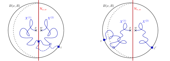
Figure 1: On the left a successful coupling. On the right, the walk $X^{(2)}$ reaches the boundary before $\mathcal{H}_{x,w}$ and the coupling fails ; note that $X^{(1)}$ could have exited $B(x,R)$ through $z^{\prime}$, hence the coupling is only a sufficient condition to have the same exit point.

We now need to control the last two expectations. First, we perform some reduction in order treat separately the events “the walk avoid the hyperplane $\mathcal{H}$” and “the walk exits through $z$”. For this, we introduce an intermediate ball $B(x,\tilde{R})$ with $\tilde{R}=\frac{1}{16}R$, and we use the strong Markov property at the hitting time $H_{\tilde{R}}^{x}$ of $\partial B(x,\tilde{R})$: we obtain the upper bound:

$$\mathbf{E}_{x}\Big{[}(\lambda_{N})^{-H_{R}^{x}}\mathbbm{1}_{\{X_{H_{R}^{x}}=z\}}\mathbbm{1}_{\{\tau>H_{R}^{w}\}}\Big{]}\leq\mathbf{E}_{x}\Big{[}(\lambda_{N})^{-H_{\tilde{R}}^{x}}\mathbbm{1}_{\{\tau>H_{\tilde{R}}^{x}\}}\Big{]}\sup_{u\in\partial B(x,\tilde{R})}\mathbf{E}_{u}\Big{[}(\lambda_{N})^{-H_{N}^{x}}\mathbbm{1}_{\{X^{1}_{H_{N}^{x}}=z\}}\Big{]}\,,$$

and similarly for the other expectation in (3.3). All together, going back to (3.1) and using (3.2) with (3.3), we obtain that the difference $|\phi_{N}(y)-\phi_{N}(x)|$ is bounded by a constant (that depends only $D$) times

$$\sum_{z\in\partial B(x,R)}\phi_{N}(z)\bigg{[}\mathbf{E}_{x}\Big{[}(\lambda_{N})^{-H_{\tilde{R}}^{x}}\mathbbm{1}_{\{\tau>H_{\tilde{R}}^{x}\}}\Big{]}+\frac{c}{N^{2}}\bigg{]}\sup_{u\in\partial B(x,\tilde{R})}\mathbf{E}_{u}\Big{[}(\lambda_{N})^{-H_{R}^{x}}\mathbbm{1}_{\{X^{1}_{H_{R}^{x}}=z\}}\Big{]}\,.$$ (3.4)

It then only remains to control the expectations appearing above, which are simple random walk estimates (by translation invariance, we can take $x=0$).

Step 3. Technical estimates and conclusion of the proof. We now state two lemmas to deal with the terms appearing in (3.4). We stress that the difficulty here comes from the term $(\lambda_{N})^{-H_{N}^{x}}$ in the expectations, which is unbounded: if this term were absent, it would be standard (gambler’s ruin and uniform exit points) estimates for random walks. In fact, we obtain comparable estimates; we postpone the proofs to Section 4, which collects some other useful random walk estimates.

Lemma 3.1 (Gambler’s ruin).

There is a constant $c_{d}$ (that depends only on the dimension) and a constant $C>0$ such that, for any $R\geq 1$ sufficiently large, we have

$$\mathbf{E}_{0}\Big{[}e^{c_{d}H_{R}/R^{2}}\mathbbm{1}_{\{\tau_{\mathcal{H}}>H_{R}\}}\Big{]}\leq\frac{C}{R}\,,$$ (3.5)

where $H_{R}$ is the hitting time of the ball $B(0,R)$ and $\tau_{\mathcal{H}}$ is the hitting time of the hyperplane $\mathcal{H}=\{z=(z_{1},\ldots,z_{d})\in\mathbb{Z}^{d},z_{1}=-1\}$ between $0$ and $-2e_{1}$.

Lemma 3.2 (Exit point).

There is a constant $c_{d}$ (that depends only on the dimension) and a constant $C>0$ such that, for any $R\geq 1$ sufficiently large, we have

$$\sup_{u\in\bar{B}(0,\frac{1}{16}R)}\mathbf{E}_{u}\Big{[}e^{c_{d}H_{R}/R^{2}}\mathbbm{1}_{\{X_{H_{R}}=z\}}\Big{]}\leq\frac{C}{R^{d-1}}\,,$$ (3.6)

where $H_{R}$ is the hitting time of the ball $B(0,R)$.

Using that $\lambda_{N}^{-1}\leq e^{c_{D}/N^{2}}$ for some constant $c_{D}$, see Lemma 2.1, we can therefore bound $(\lambda_{N})^{-H_{R}^{x}}\leq e^{c_{D}H_{R}^{x}/N^{2}}\leq e^{c_{D}\delta_{D}^{2}H_{R}^{x}/R^{2}}$ in (3.4), recalling also that we considered $R\leq\delta_{D}N$; obviously, a similarly bound holds $(\lambda_{N})^{-H_{\tilde{R}}^{x}}$. Therefore, having fixed $\delta_{D}$ small enough (how small depends on the domain $D$), we can apply Lemmas 3.1-3.2 to obtain that, for $x\sim y$,

$$|\phi_{N}(y)-\phi_{N}(x)|\leq\frac{C}{R^{d}}\sum_{z\in\partial B(x,R)}\phi_{N}(z)\,.$$

Now, Proposition 1.3 provides the bound $\phi_{N}(z)\leq cR/N$, uniformly for $z\in\partial B(x,R)$. Since we have $|\partial B(x,R)|\leq c^{\prime}R^{d-1}$, we end up with $|\phi_{N}(y)-\phi_{N}(x)|\leq C^{\prime}N^{-1}$, which concludes the proof of Theorem 1.4. ∎

Remark 3.1.

The positive reach Assumption 1 is only used in the very end of the proof, in the use of Proposition 1.3. Under the uniform cone condition Assumption 2, this has to be replaced by (2.5), see Remark 2.3. This would enables us to get $\phi_{N}(z)\leq c(R/N)^{\zeta}$ with $\zeta\in(0,1)$ in the last display, and instead of Theorem 1.4, one ends up with

$$|\phi_{N}(y)-\phi_{N}(x)|\leq Cd(x,\partial D_{N})^{\zeta-1}N^{-1}\quad\text{ for }x\sim y\,,$$

as announced in Remark 1.5.

4 Simple random walk estimates

The main goal of this section is to prove Lemmas 3.1 and 3.2, but we start with the proof of Lemma 2.2, which is a classical gambler’s ruin estimate. We will use the notation $B_{R}\vcentcolon=B(0,R)$ and we will denote $\hat{H}_{R}\vcentcolon=\min\{n\geq 0,X_{n}\in B_{R}\}$ and $\check{H}_{R}\vcentcolon=\min\{n\geq 0,X_{n}\notin B_{R}\}$, or simply $H_{R}=\check{H}_{R}$ if the random walk starts inside $B_{R}$ (according to the previous notation).

4.1 Gambler’s ruin and escaping from large balls

Let us first give a technical lemma on gambler’s ruin probabilities, that we will mostly deduce from well-known results (our key reference is [Law13]).

Lemma 4.1.

Fix $\alpha>1$. There are constants $c_{1},c_{2}$ (depending on $\alpha-1$), such that for all $R$ large enough, for all $x\in B_{\alpha R}\setminus B_{R}$, we have

$$\mathbf{P}_{x}\big{(}\hat{H}_{R}>\check{H}_{\alpha R}\big{)}\leq c_{1}\frac{d(x,B_{R})}{R}\,\,,$$ (4.1)

and also

$$\mathbf{P}_{x}\big{(}\hat{H}_{R}\wedge\check{H}_{\alpha R}\geq R^{2}\big{)}\leq c_{2}\frac{d(x,B_{R})}{R}\,.$$ (4.2)

Remark 4.1.

Lemma 4.1 is useful when the point $x$ is closer to $\partial B_{R}$ than $\partial B_{\alpha R}$. When this is not the case, we can apply the same lemma but with different balls, to obtain

$$\mathbf{P}_{x}\big{(}\hat{H}_{R}>\check{H}_{\alpha R}\big{)}\leq c_{1}^{\prime}\frac{d(x,\partial B_{\alpha R})}{R}\,,\qquad\mathbf{P}_{x}\big{(}\hat{H}_{R}\wedge\check{H}_{\alpha R}\geq R^{2}\big{)}\leq c_{2}\frac{d(x,\partial B_{\alpha R})}{R}\,.$$ (4.3)

Proof of (4.1).

We use Proposition 1.5.10 in [Law13], which gives the following estimate in dimension $d\geq 3$: let $x\in B_{\alpha R}\setminus B_{R}$, then

$$\mathbf{P}_{x}(\hat{H}_{R}<\check{H}_{\alpha R})=\frac{|x|^{2-d}-\big{(}\alpha R\big{)}^{2-d}+\bar{\mathcal{O}}(R^{1-d})}{R^{2-d}-\big{(}\alpha R\big{)}^{2-d}}\,.$$

Injecting $|x|=R+\ell$ with $\ell=|x|-R$ (we may assume that $\frac{\ell}{R}\leq 1/2$ otherwise the bound is trivial), this yields

$$\mathbf{P}_{x}(\hat{H}_{R}>\check{H}_{\alpha R})=1-\frac{(1+\ell R^{-1})^{2-d}-\alpha^{2-d}+\bar{\mathcal{O}}(R^{-1})}{1-\alpha^{2-d}}\leq c_{\alpha,d}\big{(}\ell R^{-1}+\bar{\mathcal{O}}(R^{-1})\big{)}\,,$$

which is the desired result.

In dimension $d=2$, we have from [LL10, Prop. 6.4.1] that, analogously as above,

$$\mathbf{P}_{x}(\hat{H}_{R}<\check{H}_{\alpha R})=\frac{\ln(\alpha R)-\ln|x|+\bar{\mathcal{O}}(R^{-1})}{\ln(\alpha R)-\ln R}\,.$$

Setting again $|x|=R+\ell$, we get after simplifications that

$$\mathbf{P}_{x}(\hat{H}_{R}>\check{H}_{\alpha R})=\frac{\ln(1+\ell R^{-1})+\bar{\mathcal{O}}(R^{-1})}{\ln\alpha}\leq c_{\alpha,d}\big{(}\ell R^{-1}+\bar{\mathcal{O}}(R^{-1})\big{)}\,,$$

as needed. ∎

Proof of (4.2).

The proof relies on the usual martingale argument. We fix some $x\in B_{\alpha R}\setminus B_{R}$ such that $|x|-R\leq\delta R$, with $\delta=\delta_{\alpha}<\frac{1}{2}\alpha$ small enough (but fixed) so that in (4.1) we have $\mathbf{P}_{x}(\hat{H}_{R}<\check{H}_{\alpha R})\leq\frac{1}{2}$; note that the bound (4.2) is trivial in the case $|x|-R>(2c_{1})^{-1}R$.

Let us write for simplicity $T\vcentcolon=\min\{\hat{H}_{R},\check{H}_{\alpha R}\}$, and consider the martingale $|X_{t\wedge T}|^{2}-t\wedge T$. Applying the stopping time theorem, we get that

$$|x|^{2}=\mathbf{E}_{x}\big{[}|X_{t\wedge T}|^{2}-t\wedge T\big{]}\xrightarrow[]{t\uparrow\infty}\mathbf{E}_{x}\big{[}|X_{T}|^{2}-T\big{]}\,,$$ (4.4)

where we have used dominated and monotonous convergence as we took the limit $t\uparrow\infty$. Splitting the last expectation according to whether $X_{T}\in B_{R}$ or not, we have

$$|x|^{2}=\mathbf{P}_{x}\big{(}X_{T}\in B_{R}\big{)}\mathbf{E}_{x}\big{[}|X_{T}|^{2}-T\,\big{|}\,X_{T}\in B_{R}\big{]}+\mathbf{P}_{x}\big{(}X_{T}\notin B_{R}\big{)}\mathbf{E}_{x}\big{[}|X_{T}|^{2}-T\,\big{|}\,X_{T}\notin B_{R}\big{]}\,.$$

Rearranging the terms, we obtain

$$\mathbf{P}_{x}\left(X_{T}\in B_{R}\right)\mathbf{E}_{z}\left[T\,\big{|}\,X_{T}\in B_{R}\right]=\mathbf{P}_{x}\left(X_{T}\in B_{T}\right)\mathbf{E}_{x}\left[|X_{T}|^{2}-|x|^{2}\,\big{|}\,X_{T}\in B_{R}\right]\\ +\mathbf{P}_{x}\left(X_{T}\not\in B_{R}\right)\mathbf{E}_{x}\left[|X_{R}|^{2}-T-|x|^{2}\,\big{|}\,X_{T}\not\in B_{R}\right]\,.$$

Since we took $x\notin B_{R}$, on the event $\left\{X_{T}\in B_{R}\right\}$ we have $|X_{T}|^{2}\leq|x|^{2}$, so we can bound the first term by $0$. Using also that $T\geq 0$, we end up with

$$\mathbf{P}_{x}\left(X_{T}\in B_{T}\right)\mathbf{E}_{x}\left[T\,\big{|}\,X_{T}\in B_{R}\right]\leq\mathbf{P}_{x}\left(X_{T}\notin B_{R}\right)\mathbf{E}_{x}\left[|X_{T}|^{2}-|x|^{2}\,\big{|}\,X_{T}\notin B_{R}\right]\,.$$

Note that on the event $\left\{X_{T}\notin B_{R}\right\}$ and since we have fixed $x$ verifying $|x|-R\leq\delta R$, we have $|X_{T}|^{2}-|x|^{2}\leq c_{\alpha}R^{2}$, and recall that we chose $\delta$ small enough so that $\mathbf{P}_{x}\left(X_{T}\in B_{R}\right)\geq\frac{1}{2}$ in (4.1). Therefore, we obtain

$$\mathbf{E}_{x}\left[T\,|\,X_{T}\in B_{R}\right]\leq 2c_{\alpha}R^{2}\mathbf{P}_{z}\left(X_{T}\not\in B_{R}\right)\leq 2c_{\alpha}c_{1}R(|x|-R)\,,$$ (4.5)

where we have used (4.1) for the last inequality. We thus get

$$\begin{split}\mathbf{P}_{x}(T>R^{2})&=\mathbf{P}_{x}(X_{T}\in B_{R})\mathbf{P}_{x}\big{(}T>R^{2}\,|\,X_{T}\in B_{R}\big{)}+\mathbf{P}_{x}(X_{T}\notin B_{R})\mathbf{P}_{x}\big{(}T>R^{2}\,|\,X_{T}\notin B_{R}\big{)}\\ &\leq\mathbf{P}_{x}\big{(}T>R^{2}\,|\,X_{T}\in B_{R}\big{)}+\mathbf{P}_{x}(X_{T}\notin B_{R})\leq 4c_{\alpha}c_{1}\frac{|x|-R}{R}+c_{1}\frac{|x|-R}{R}\,,\end{split}$$

where in the last line we have used Markov’s inequality together with (4.5) for the first term, and (4.1) for the second term. This concludes the proof of (4.2). ∎

We are now ready to conclude the proof of Lemma 2.2, thanks to Assumption 1.

Proof of Lemma 2.2.

Using the positive reach Assumption 1, there is some $\varepsilon_{0}>0$ for which, for all $x\in D_{N}$, there exists $z\notin D_{N}$ such that the ball $B(z,\varepsilon_{0}N)$ is in $D_{N}^{c}$ and $d(x,B(z,\varepsilon_{0}N))\leq 2d(x,\partial D_{N})$. Now, let $A$ be large enough, so that $D_{N}\subset B(z,AN)$.

Now, we simply observe that $H_{\partial D_{N}}\leq\min\{H_{B(z,\varepsilon_{0}N)},H_{B(z,AN)^{c}}\}$, so that using Lemma 4.1-(4.2) (with $\alpha\vcentcolon=A/\varepsilon_{0}$), we get that

$$\mathbf{P}_{x}(H_{\partial D_{N}}>N^{2})\leq c\frac{B(z,\varepsilon_{0}N)}{\varepsilon_{0}N}\leq c^{\prime}\frac{d(x,\partial D_{N})}{N}\,.$$

This concludes the proof of Lemma 2.2. ∎

4.2 Proof of Lemma 3.1

The proof will mostly rely on Lemma 4.1. Decomposing over the value of the integer part of $R^{-2}H_{R}$, we get the bound

$$\mathbf{E}_{0}\Big{[}e^{c_{d}H_{R}/R^{2}}\mathbbm{1}_{\{\tau_{\mathcal{H}}>H_{R}\}}\Big{]}\leq e^{c_{d}}\mathbf{P}_{0}\big{(}\tau_{\mathcal{H}}>H_{R}\big{)}+\sum_{k\geq 1}e^{c_{d}(k+1)}\mathbf{P}_{0}\big{(}\tau_{\mathcal{H}}>H_{R}\geq kR^{2}\big{)}\,.$$

For any $k\geq 1$, we can use the Markov property at time $R^{2}$ to get that

$$\mathbf{P}_{0}\big{(}\tau_{\mathcal{H}}>H_{R}\geq kR^{2}\big{)}\leq\mathbf{P}_{0}\big{(}\tau_{\mathcal{H}}\wedge H_{R}\geq R^{2}\big{)}\sup_{v\in B_{R}}\mathbf{P}_{v}\big{(}H_{R}\geq(k-1)R^{2}\big{)}\\ \leq\mathbf{P}_{0}\big{(}\tau_{\mathcal{H}}\wedge H_{R}\geq R^{2}\big{)}\times(\gamma_{R})^{k-1}\,,$$

where we have set $\gamma_{R}\vcentcolon=\sup_{v\in B_{R}}\mathbf{P}_{v}(H_{R}\geq R^{2})$ and again applied the Markov property iteratively; note that we have $\gamma_{R}\leq\gamma_{d}<1$ uniformly in $R$ large enough by the invariance principle (we have $\lim_{R\to\infty}\gamma_{R}=\mathbf{P}_{0}(\sup_{s\in[0,1]}|B_{s}|<1)$ with $B$ a Brownian motion). All together, we obtain that

$$\mathbf{E}_{0}\Big{[}e^{c_{d}H_{R}/R^{2}}\mathbbm{1}_{\{\tau_{\mathcal{H}}>H_{R}\}}\Big{]}\leq e^{c_{d}}\mathbf{P}_{0}\big{(}\tau_{\mathcal{H}}>H_{R}\big{)}+\mathbf{P}_{0}\big{(}\tau_{\mathcal{H}}\wedge H_{R}\geq R^{2}\big{)}\sum_{k\geq 1}e^{c_{d}}(e^{c_{d}}\gamma_{d})^{k}\,,$$

and the last sum is bounded by a constant if we choose for instance $c_{d}\vcentcolon=\frac{1}{2}\ln\gamma_{d}^{-1}$ so that $e^{c_{d}}\gamma_{d}=\gamma_{d}^{1/2}<1$. It therefore remains to estimate the two probabilities in the above display.

In order to be in position to apply Lemma 4.1, we introduce some new sets. Let $z\in\mathbb{Z}^{2}$ be such that the ball $\tilde{B}_{R/2}\vcentcolon=B(z,\frac{1}{2}R)$ of radius $R/2$ is tangent to $\mathcal{H}$ on the other side of $0$ (so in particular $d(0,\tilde{B}_{R/2})=1$), and let also $\tilde{B}_{R}\vcentcolon=B(z,R)$ and $\tilde{B}_{2R}\vcentcolon=B(z,2R)$. Then, starting from $0$, by construction we have that $H_{R}\geq H_{\partial\tilde{B}_{R}}$ on the event $\tau_{\mathcal{H}}>H_{R}$, and also $\tau_{\mathcal{H}}\leq H_{\tilde{B}_{R/2}}$, so that we get

$$\mathbf{P}_{0}\big{(}\tau_{\mathcal{H}}>H_{R}\big{)}\leq\mathbf{P}_{0}\big{(}\tau_{\mathcal{H}}>H_{\partial\tilde{B}_{R}}\big{)}\leq\mathbf{P}_{0}\big{(}H_{\tilde{B}_{R/2}}>H_{\partial\tilde{B}_{R}}\big{)}\leq\frac{c}{R}\,.$$

For the last inequality, we have used Lemma 4.1-(4.1) (with $\alpha=2$).

On the other hand, we also have by construction that $H_{\tilde{B}_{R/2}}\wedge H_{\partial\tilde{B}_{2R}}\geq\tau_{\mathcal{H}}\wedge H_{R}$, so by Lemma 4.1-(4.2) (with $\alpha=4$), we obtain

$$\mathbf{P}_{0}\big{(}\tau_{\mathcal{H}}\wedge H_{R}\geq R^{2}\big{)}\leq\mathbf{P}_{0}\big{(}H_{\tilde{B}_{R/2}}\wedge H_{\partial\tilde{B}_{2R}}\geq(R/2)^{2}\big{)}\leq\frac{c^{\prime}}{R}\,.$$

This concludes the proof of Lemma 3.1. ∎

4.3 Proof of Lemma 3.2

To prove Lemma 3.2, we use a classical result for the simple random walk: for $R>1$ large enough, the random walk starting from a point inside $B_{R/4}$ has a roughly uniform exit point of $B_{R}$. This is Lemma 6.3.7 in [LL10], that we state here with our notation for the reader’s convenience. There exists a constant $c_{3}$ such that, for any $R$ large enough,

$$\sup_{u\in\bar{B}_{R/4}}\sup_{z\in\partial B_{R}}\mathbf{P}_{u}\big{(}X_{H_{R}}=z\big{)}\leq\frac{c_{3}}{R^{d-1}}\,.$$ (4.6)

As for the proof of Lemma 3.1, we start by decomposing over the value of $R^{-2}H_{R}$ (over even integers this time), to obtain, for $u\in B_{R/32}$,

$$\mathbf{E}_{u}\left[e^{c_{d}H_{R}/R^{2}}\mathbbm{1}_{\{X_{H_{R}}=z\}}\right]\leq e^{2c_{d}}\mathbf{P}_{u}(X_{H_{R}}=z)+\sum_{k\geq 1}e^{2c_{d}(k+1)}\mathbf{P}_{u}\big{(}H_{R}\geq 2kR^{2},X_{H_{R}}=z\big{)}\,.$$ (4.7)

Using (4.6), the first term is bounded by $c_{3}R^{-(d-1)}$, uniformly in $u\in B_{R/32}$ and $z\in\partial B_{R}$.

For the terms $k\geq 1$ in the sum, we use the Markov property at time $H_{R/4}$, and we decompose according to whether $H_{R/4}\geq kR^{2}\geq k(R/2)^{2}$ or $H_{R/4}<kR^{2}$. The first case is

$$\mathbf{P}_{u}\Big{(}H_{R/4}\geq kR^{2},H_{R}\geq 2kR^{2},X_{H_{R}}=z\Big{)}\leq\mathbf{P}_{u}\Big{(}H_{R/4}\geq k(R/2)^{2}\Big{)}\sup_{v\in\partial B_{R/4}}\mathbf{P}_{v}\left(X_{H_{R}}=z\right)\\ \leq(\gamma_{d})^{k}\times\frac{c_{3}}{R^{d-1}}\,,$$ (4.8)

where we have used (4.6) for the second factor and also that the first factor is bounded by $(\gamma_{R/2})^{k}$ with $\gamma_{r}\vcentcolon=\sup_{v\in B_{r}}\mathbf{P}_{v}(H_{r}\geq r^{2})\leq\gamma_{d}<1$ similarly as in the proof of Lemma 3.1.

For the second case, we decompose over the exit point of $B_{R/4}$ to obtain

$$\mathbf{P}_{u}\Big{(}H_{R/4}<kR^{2},H_{R}\geq 2kR^{2},X_{H_{R}}=z\Big{)}\leq\sum_{v\in\partial B_{R/4}}\mathbf{P}_{u}(X_{H_{R/4}}=v)\mathbf{P}_{v}\left(X_{H_{R}}=z,H_{R}\geq kR^{2}\right)\,,$$ (4.9)

with $\mathbf{P}_{u}(X_{H_{R/4}}=v)\leq c_{3}^{\prime}R^{-(d-1)}$ uniformly for $u\in\bar{B}_{R/16}$ and $v\in\partial B_{R/4}$, thanks to (4.6). For the last term, we decompose over the exit time to write, for any $z\in\partial B_{R}$,

$$\mathbf{P}_{v}\Big{(}X_{H_{R}}=z,H_{R}\geq kR^{2}\Big{)}=\sum_{i\geq kR^{2}}\mathbf{P}_{v}\left(X_{i}=z,H_{R}=i\right)=\sum_{i\geq kR^{2}}\mathbf{P}_{z}\left(X_{i}=v,\bar{H}_{R}\geq i\right)\,,$$

where we have used the reversibility of the simple random walk for the last equality, and denoted $\bar{H}_{R}=\bar{H}_{\partial B_{R}}$ with $\bar{H}_{\Lambda}\vcentcolon=\min\{n\geq 1,X_{n}\in\Lambda\}$. We therefore have that

$$\begin{split}\sum_{v\in\partial B_{R/4}}\mathbf{P}_{v}\left(X_{H_{R}}=z,H_{R}\geq kR^{2}\right)&=\sum_{i\geq kR^{2}}\mathbf{P}_{z}\big{(}\bar{H}_{R}\geq i,X_{i}\in\partial B_{R/4}\big{)}\\ &\leq\mathbf{E}_{z}\bigg{[}\mathbbm{1}_{\{\bar{H}_{R}\geq kR^{2}\}}\sum_{j\geq 0}\mathbf{P}_{X_{kR^{2}}}\big{(}X_{j}\in\partial B_{R/4},H_{R}\geq j\big{)}\bigg{]}\,,\end{split}$$

where we have used the Markov property at time $kR^{2}$ for the last identity. Now, defining $G_{R}(x,A)\vcentcolon=\mathbf{E}_{x}\big{[}\sum_{j=0}^{\bar{H}_{R}}\mathbbm{1}_{\{X_{j}\in A\}}\big{]}$ the Green function for the random walk killed upon exiting $B_{R}$, we get that

$$\sum_{j\geq 0}\mathbf{P}_{x}\big{(}X_{j}\in\partial B_{R/4},H_{R}\geq j\big{)}=G_{R}(x,\partial B_{R/4})\leq\sup_{w\in\partial B_{R/4}}G_{R}(w,\partial B_{R/4})\,.$$

Now, by Lemma 4.1-(4.1), the number of visits to $\partial B_{R/4}$ before exiting $B_{R}$ is dominated by a geometric random variable with parameter $\sup_{w\in\partial B_{R/4}}\mathbf{P}_{w}(\bar{H}_{\partial B_{R/4}}<\check{H}_{R})\leq 1-cR^{-1}$. We therefore get that $G_{R}(w,\partial B_{R/4})\leq c^{\prime}R$ which, going back to (4.9) gives the following bound:

$$\mathbf{P}_{u}\Big{(}H_{R/4}<kR^{2},H_{R}\geq 2kR^{2},X_{H_{R}}=z\Big{)}\leq\frac{c_{3}^{\prime}}{R^{d-1}}\times\mathbf{P}_{z}\big{(}\bar{H}_{R}\geq kR^{2}\big{)}\times c^{\prime}R\,.$$

It remains to deal with the last probability. We write, for $z\in\partial B_{R}$,

$$\mathbf{P}_{z}\big{(}\bar{H}_{R}\geq kR^{2}\big{)} \leq\mathbf{P}_{z}\big{(}\hat{H}_{R/2}<R^{2},\bar{H}_{R}\geq kR^{2}\big{)}+\mathbf{P}_{z}\big{(}\hat{H}_{R/2}>R^{2},\bar{H}_{R}\geq kR^{2}\big{)}$$

$$\leq\Big{(}\mathbf{P}_{z}\big{(}\hat{H}_{R/2}<R^{2}\leq\bar{H}_{R}\big{)}+\mathbf{P}_{z}\big{(}\hat{H}_{R/2}\wedge\bar{H}_{R}\geq R^{2}\big{)}\Big{)}\sup_{v\in B_{R}}\mathbf{P}_{v}\big{(}\bar{H}_{R}\geq(k-1)R^{2}\big{)}\,,$$

where we have applied the Markov property at time $R^{2}$ for the second inequality. Lemma 4.1 (more precisely, see Remark 4.1-(4.3)) gives that the first two terms are bounded by a constant times $R^{-1}$, whereas the last term is bounded by $(\gamma_{d})^{k-1}$, as in the proof of Lemma 3.1. We therefore end up with the upper bound

$$\mathbf{P}_{u}\Big{(}H_{R/4}<kR^{2},H_{R}\geq 2kR^{2},X_{H_{R}}=z\Big{)}\leq\frac{C}{R^{d-1}}(\gamma_{d})^{k-1}\,.$$ (4.10)

Plugging (4.8)-(4.10) in (4.7), we finally conclude that

$$\mathbf{E}_{u}\left[e^{c_{d}H_{R}/R^{2}}\mathbbm{1}_{\{X_{H_{R}}=z\}}\right]\leq\frac{C}{R^{d-1}}\Big{(}e^{2c_{d}}+\sum_{k=1}^{\infty}e^{2c_{d}(k+1)}(\gamma_{d})^{k-1}\Big{)}\,,$$

which concludes the proof if we choose $c_{d}\vcentcolon=\frac{1}{4}\ln\gamma_{d}^{-1}$, so that the last sum is bounded by a constant. ∎

Acknowledgments. The authors would like to thank Antoine Mouzard for numerous, enthusiastic, enlightening discussions. We would also like to thank Karine Beauchard and Monique Dauge for helpful pointers to some of the literature. Both authors also acknowledge the support of grant ANR Local (ANR-22-CE40-0012).

References

• [BH68] JH Bramble and BE Hubbard β€œEffects of boundary regularity on the discretization error in the fixed membrane eigenvalue problem” In SIAM Journal on Numerical Analysis 5.4 SIAM, 1968, pp. 835–863
• [Bol94] Erwin Bolthausen β€œLocalization of a two-dimensional random walk with an attractive path interaction” In The Annals of Probability, 1994, pp. 875–918
• [Bou24] Nicolas Bouchot β€œA confined random walk locally looks like tilted random interlacements”, 2024 arXiv:2405.14329 [math.PR]
• [Bou24a] Nicolas Bouchot β€œCovering time for the confined walk in large domains” In preparation, 2024+
• [Cia02] Philippe G Ciarlet β€œThe finite element method for elliptic problems” SIAM, 2002
• [CR73] Philippe G Ciarlet and P-A Raviart β€œMaximum principle and uniform convergence for the finite element method” In Computer methods in applied mechanics and engineering 2.1 Elsevier, 1973, pp. 17–31
• [Din+21] Jian Ding, Ryoki Fukushima, Rongfeng Sun and Changji Xu β€œDistribution of the Random Walk Conditioned on Survival among Quenched Bernoulli Obstacles” In The Annals of Probability 49.1, 2021 DOI: 10.1214/20-AOP1450
• [Kut70] James R Kuttler β€œFinite difference approximations for eigenvalues of uniformly elliptic operators” In SIAM Journal on Numerical Analysis 7.2 SIAM, 1970, pp. 206–232
• [Law13] Gregory F Lawler β€œIntersections of random walks”, Modern BirkhΓ€user Classics Springer Science & Business Media, 2013 DOI: 10.1007/978-1-4614-5972-9
• [LL10] Gregory F. Lawler and Vlada Limic β€œRandom Walk: A Modern Introduction” Cambridge University Press, 2010 DOI: 10.1017/CBO9780511750854
• [SW77] Alfred H Schatz and Lars B Wahlbin β€œInterior maximum norm estimates for finite element methods” In Mathematics of Computation 31.138, 1977, pp. 414–442