Surrogate Models studies for laser-plasma accelerator electron source design through numerical optimisation

Abstract

The optimisation of the plasma target design for high quality beam laser-driven plasma injector electron source relies on numerical parametric studies using Particle in Cell (PIC) codes. The common input parameters to explore are laser characteristics and plasma density profiles extracted from computational fluid dynamic studies compatible with experimental measurements of target plasma density profiles. We demonstrate the construction of surrogate models using machine learning technique for a laser-plasma injector (LPI) electron source based on more than $12000$ simulations of a laser wakefield acceleration performed for sparsely spaced input parameters [1]. Surrogate models are very interesting for LPI design and optimisation because they are much faster than PIC simulations. We develop and compare the performance of three surrogate models, namely, Gaussian processes (GP), multilayer perceptron (MLP), and decision trees (DT). We then use the best surrogate model to quickly find optimal working points to get a selected electron beam energy, charge and energy spread using different methods, namely random search, Bayesian optimisation and multi-objective Bayesian optimisation.

I Introduction

Laser wakefield acceleration (LWFA)[2] is a promising method that can produce high-energy electrons within compact structures. It can achieve peak accelerating electric field in the order of $100\,$GV/m, $3$ order of magnitude higher than the fields generated by RF accelerators [3]. Furthermore, LWFA produces electrons with extremely short pulse duration [4], typically around 10’s of femtoseconds. This short electron bunch length is particularly advantageous for applications like radiotherapy techniques such as FLASH [5] and the creation of coherent X-rays using free electron laser [6]. In the past two decades several groups were able to generate electrons beams with desired properties such as high energy [7], high charge [8], low energy spread [9], low emittance [10]. However, these electron beams may not display all these properties simultaneously. This is due to the highly non-linear and coupled nature of the laser wakefield interaction, making particularly difficult to obtain a stable electron beam with demanding features.

The nonlinear nature of LWFA makes the use of numerical modelling such as Particle in Cell (PIC) simulations [11] necessary for designing reliable accelerators, which can be intractable if one relies only on experience and scaling laws. This is why machine learning (ML) techniques [12] are increasingly used in LWFA studies and experiments. In fact, recent papers [13, 14] showed that optimal working points can be obtained by using a Bayesian optimisation approach. In this article we present surrogate models (SM) of an LPI [12], describe the construction of these models and discuss important aspects for generating efficient SM. We then evaluate and compare their performances. Finally, we illustrate how to use these SM to find optimal working points and stable operation regions of an LPI. Indeed, with their low computational cost in comparison to PIC simulations, SM are better suited to quickly probe different configurations of an LPI.

II Numerical experiments

The data set used for the training of the SM comes from PIC simulations from a previous design study of input parameters set up to optimise a future LPI at IJCLab described in [1] , which aims to deliver electron beams ranging from $150-250\,$ MeV, with $30-50\,$pC of charge, an energy spread lower than $5\%$ and an emittance of less than $2\,$mm.mrad. The laser driver considered is provided by the LASERIX platform at IJCLab with a laser power in the range of $40$ to $80\,$TW. The LPI relies on an ionisation injection scheme [15] with a plasma target divided into two regions [16]. The first region is composed of a gas mixture of $He$ doped with $N_{2}$ whose length is $0.6\,$mm allowing for the injection of the inner shell electrons of N⁵⁺ and N⁶⁺. The second region is composed of pure He, $1.2\,$mm long and dedicated to the acceleration of the injected electrons.

To summarise the main objectives that we are pursuing in these numerical experiments are: (i) construct a classification-based model that predicts electron beam injection as a function of input parameters; (ii) Construct ML-based SM from simulation data that are able to predict the LPI electron beam parameters; (iii) Use both classification model and SM to optimise LPI configurations and investigate the stability of optimal beam parameters.

Figure 1: Surrogate models and injection prediction based LPI design optimisation studies flowchart. The dashed line represents potential optimisation loop update of the input $x^{(i)}$.

The scheme in Figure Fig 1 illustrates the principle of the numerical experiments. An LPI configuration input $x^{(i)}$ can be filtered by an injection prediction model, providing inputs for the LPI SM to predict the electron beam parameters $y^{(j)}$. An objective function $f$ built from the outputs $y^{(j)}$ can feed an optimisation routine.

III Data sets generation

Two large data sets of LPI simulations were produced using the SMILEI[17] PIC code with azimuthal mode decomposition, envelope approximation[18, 19, 20] and a low number of particles per cell (PPC). A single run is performed in $130\,$core-hours at the GENCI High performance computing (HPC) Irene Joliot Curie facility [21], compared to $450\,$core-hours for more standard settings with higher number of PPC using envelope and azimuthal mode decomposition. The reduced number of PPC only had a modest impact on the simulation results, as specified in [1]. The simulation data are available online [22]. The simulations had a set of 4 input variable parameters namely: $x^{(i)}=(a_{0},x_{off},p_{1},c_{N_{2}})$ with $a_{0}$ the laser pulse normalised vector potential in vacuum, $x_{off}$ the laser focal position in vacuum, $p_{1}$ the gas pressure in the first region and $c_{N_{2}}$ the concentration of nitrogen in the same region. It is important to notice that the pressure in the second region was kept equal to the one in the first region $p_{1}\simeq p_{2}$, the difference of pressure between the two chambers came from the dopant concentration in the first region. The reference position $x_{off}=0$ corresponds to the entrance of the second chamber [23]. The input parameters $x^{(i)}$ can vary up to the value indicated in Tab. 1. The maximum value of $a_{0}$ is $1.85$, which is lower than the barrier suppression ionisation potential threshold for the two inner shell electrons of $N$. For injection to occur with these simulations self-focusing was thus mandatory.

$a_{0}$	$x_{off}$ [$\mu$m]	$p_{1}$ [mbar]	$c_{N_{2}}$ [$\%$]
$[1.1,1.85]$	$[-400,1800]$	$[14,119]$	$[0.2,12]$

Table 1: Interval for the 4 input parameters used of the random scan simulations

We chose 4 output parameters to characterise the electron beam, namely: $y^{(j)}=(E_{med},\delta E_{mad},Q,\epsilon_{y})$. $E_{med}$ is the median energy, $\delta E_{mad}=\sigma_{mad}/E_{med}$ with $\sigma_{mad}$ the median absolute deviation, $Q$ the charge and $\epsilon_{y}$ the transverse normalised emittance. The laser driver was linearly polarised along the $y$-axis. The output parameters $y^{(j)}$ used as validation data in the model were evaluated only at the last time-step of the simulation, they thus represent the features of the beam right after the plasma outramp. The first simulations dataset set1 consists of five massive random scans, each with $2401$ configurations. Each random scan explored a part of the input parameter space using either a continuous uniform distribution or a skew normal distribution. These random scans resulted in some intervals of the input space being over represented in the dataset. The histograms in Fig. 2 present the configurations distribution of the inputs $x^{(i)}$.

The density of points within the random scan dataset set1 was high enough to explore finely the input parameters space, to which the output might be very sensitive. The resolution of the input space with the random scan dataset set1 is largely above the one we can obtain with experimental devices even with the most refined diagnostics. For example with $x_{off}$ we reach a numerical resolution as low as $1\,\mu$m where as it is barely $50\,\mu$m in standard experimental conditions.

data set	$E_{med}$ [MeV]	$\delta E_{mad}$ [%]	$Q$ [pC]	$\epsilon_{y}$ [mm.mrad]
set1	$[28,355]$	$[0.03,71]$	$[10^{-5},900]$	$[6\times 10^{-4},85]$
set2	$[29,371]$	$[0.08,75]$	$[6\times 10^{-4},968]$	$[2.5\times 10^{-3},81]$

Table 2: Interval for the 4 output electron beam parameters of the simulations dataset

A second simulations dataset set2 was produced using an injection prediction model (see IV.1) for filtering input parameters $x^{(i)}$ resulting in $3700$ simulations. For the set2 data the input parameters $x^{(i)}$ were randomly drawn from the intervals presented in Tab. 1 using a continuous uniform distribution (Fig. 2).

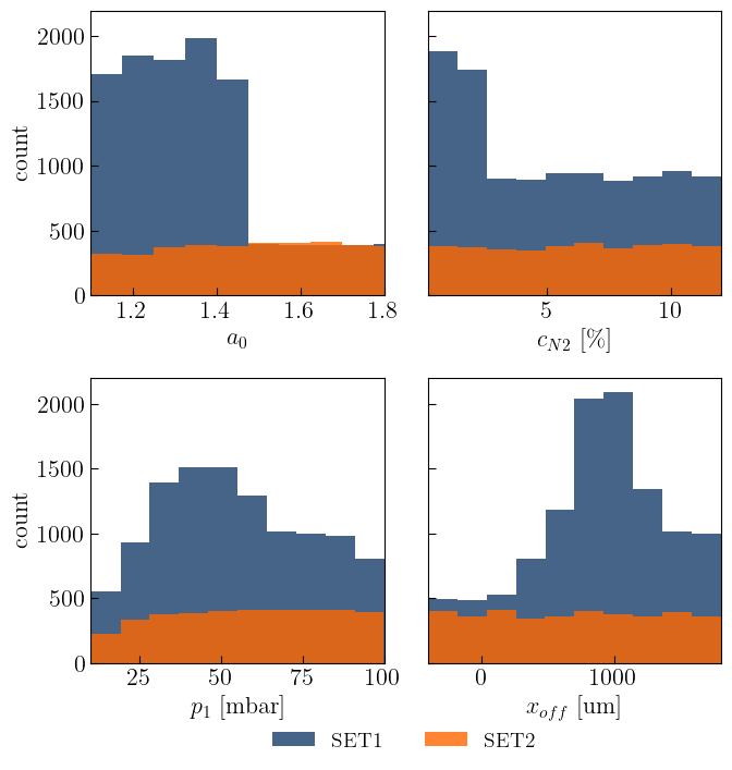
Figure 2: Distribution of the input parameters for the $10977$ training data simulations (blue) and the $3700$ test data simulations (orange).

For the set1, out of the $12004$ simulations, $10977$ resulted in injected beams. The output $y^{(j)}$ ranges are presented in Tab.2 for both data set set1 and set2. The two data set were used both as training data or test data.

IV Model construction

The current section intends to present the training process of the models and the importance of the input parameter distribution in the training dataset.

IV.1 Injection prediction model

We constructed an injection model trained on the initial dataset SET1. This model aims at predicting whether injection will happen or not for the input $x^{(i)}$. This model uses a simple random forest algorithm to make its prediction, the performance of the model is $98$%. This injection prediction model can save computational time before launching new simulations or as a constraint in the Bayesian optimisation search to filter the input parameters. Fig. 3 shows, as a function of the input parameter ($a_{0}$,$p_{1}$), in blue the points corresponding to no injection, in orange beams for which injection occurs. The definition of injection is an accelerated beam ($\gamma_{z}>10$) with charge $Q>0.03\,$fC. The black curve corresponds to the critical pressure for self-focusing as defined in [1, 24].

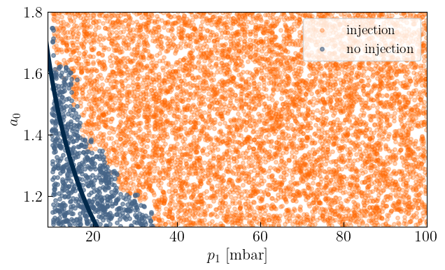
Figure 3: Injection model tested on randomly generated points. The dark-blue curve is the critical pressure necessary for self focusing.

It can be seen that the injection condition determined by the model is proportional to the theoretical limit set by the self-focusing threshold. However electron injection by ionisation from N⁵⁺ and N⁶⁺ limit is greater than the critical pressure for self-focusing, given the limited intensity assumed for the laser driver pulse in the study, $a_{0}\in[1.1,1.85]$.

IV.2 LPI model

We aim to study and compare various ML methods and eventually determine which one would be the most appropriate to model and optimise the LPI. The methods considered are:

• Neural network (NN) like multilayer perceptron (MLP) – which is a well-generalised robust method for learning nonlinear data

• Trees like Extreme gradient boosting (XGB)– a classical method for learning by splitting data into different branches. These methods are fast but tend to overfit [25].

• Gaussian Processes (GP) - which is a statistical method allowing the prediction of the expected value and its variance. It has no hyper-parameters to tune after the Kernel and length are defined. It is at the core of Bayesian Optimisation, which has been successfully used in multiple accelerator physics applications and studies [13].

IV.2.1 multilayer perceptron (MLP)

The first method used to generate a surrogate model of the LPI was a MLP. The MLP was implemented using Tensorflow and Keras python library [26]. The MLP used is a model consisting of $5$ layers, $1$ input layer with $4$ neurons, $1$ output layer with $4$ neurons, and $3$ intermediate layers with 64 neurons. Each layer has a $20\%$ dropout rate. We used the function PRELU [27] as an activation function for the $3$ intermediate layers and a sigmoid function for the last layer. Altogether this model contains $9092$ trainable parameters. This model was trained on $200$ epochs with a batch size of $50$. The loss function used was the mean squared error (MSE). To avoid over-fitting we also used a K-fold cross validation method [28].

IV.3 Extreme gradient boosting (XGB)

We implemented this method by using the xgboost library[29]. The maximum tree depth was set to $10$, the loss function was also MSE in this case. We used K-fold cross validation.

IV.3.1 Gaussian Process (GP)

We implemented this method by using the Gpy library [30]. The kernel used was Matérn, which is generalisation of Gaussian radial basis function, and allows to capture physical processes due to double differentiability by the choice of a smoothness parameter $\nu=2.5$.

The training process on a high-performance laptop is relatively quick, it takes only a few seconds for the XGB model and a few minutes for the GP and MLP models. Additionally, the computation time for LPI configurations is significantly shorter compared to low-fidelity simulations on HPC cpu nodes. The MLP, XGB, and GP models are approximately $10^{7}$ , $10^{8}$, $10^{6}$ times faster than simulations, respectively.

It is important to note that for all models (MLP,XGB,GP), we need to rescale the outputs as well as the inputs from $0$ to $1$ to get the most accurate results. The output parameters, $y^{(i)}$, are scaled so that the calculation of the loss function is well weighted which corresponds to the same magnitude in all of the outputs.

IV.3.2 Importance of the input parameters distribution

All three models MLP, XGB, and GP were tested on the set2 data, consisting of 3700 test points, separate from the 10977 samples of set1 used for training. We observe that the coefficient of determination $R^{2}$ between the SM predictions and the outputs of set2 is above 0.9. However, this score significantly decreases in regions where the density of training points is lower than 1. The density is defined as the number of points inside an hypercube of a side $0.1$ in the normalised hyper space.

We propose a reliability criteria for the SM models based on the relation between $R^{2}$ and $MSE$ :

$$R^{2}=1-\frac{\sum_{i=1}^{4}\sum_{j=1}^{N}(y_{ij}-f_{ij})^{2}}{\sum_{i=1}^{4}\sum_{j=1}^{N}(y_{ij}-\bar{y}_{i})^{2}}=$$ (1)

$$1-\frac{4\sum_{j=1}^{N}MSE_{j}}{\sum_{i=1}^{4}\sum_{j=1}^{N}(y_{ij}-\bar{y}_{i})^{2}}$$

With $y$: output value of the test data, $f$: predicted value by the surrogate, $\bar{y}$: simulation mean value for a batch of size $N$. The index $i$ represents the 4 output parameters, $j$ represents the test points.

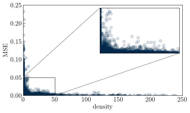
Figure 4: Scatter plot showing the relationship between density of input data configuration points and MSE for every test point. The blue points represents the different configurations.

The relationship between $MSE$ and $R^{2}$ can be used to define a reliability criteria for the test points in a given region of the input parameter space. We observe that $R^{2}\geq 0.9$ for a given batch corresponds to $MSE<5.10^{-3}$ and that the probability of getting a small $MSE$ increases with the local density of training points as shown in Fig. 4. Thus to be confident that $R^{2}\geq 0.9$ in every region of the 4-dimensional input space we need to have a high enough density which was unfortunately not the case for at least $30\%$ of the parameter space when using the simulation data of SET1 [1] as training. This is why in the following the models were trained with data from SET2 uniformly distributed points and tested on the data of SET1. As shown in Fig. 5, 6 a better homogeneity largely compensates the reduction of the number of training points for our LPI SM.

V Results

V.1 Performances of surrogate models

The SM trained on the data set2 showed good correlation with MLP, XGB and GP model having an $R^{2}$ score of $0.98$, $0.95$ and $0.98$, respectively, across all output parameters. However, as shown in Table 3, the median energy and charge are consistently better predicted by the models compared to $\delta E_{mad}$ and $\epsilon_{y}$.

	$E_{med}$	$\delta E_{mad}$	$Q$	$\epsilon_{y}$
MLP	0.99	0.97	0.99	0.95
XGB	0.97	0.93	0.97	0.91
GP	0.99	0.98	0.99	0.96
interpolation	0.9	0.9	0.94	0.87

Table 3: $R^{2}$ correlation score for the different surrogate models

Figure 5 illustrates that the MLP and GP model begin to converge to $R^{2}=0.99$ with a training size of approximately $500\,$samples. All SM outperform a simple interpolation model,which only reaches a correlation score of $R^{2}=0.9$ when the training size exceeds 3,000 samples..

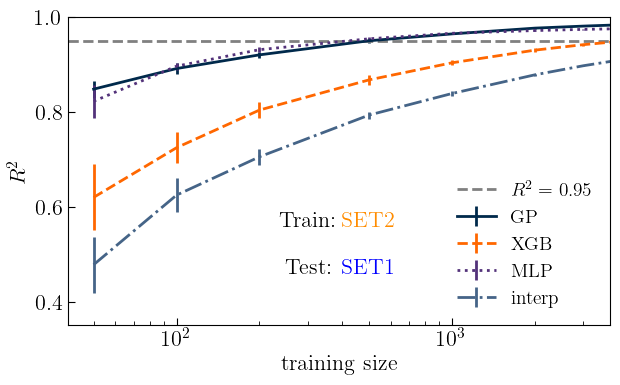
Figure 5: coefficient of determination $R^{2}$ as a function of the training size in log scale, for all the SM trained on SET2 and tested on SET1. $R^{2}$ was taken as the average over 10 training sessions, with the vertical bars representing the standard deviation

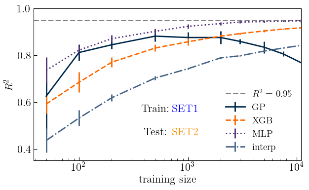
Figure 6: coefficient of determination $R^{2}$ as a function of the training size in log scale, for all the SM trained on SET1 and tested on SET2. $R^{2}$ was taken as the average over 10 training sessions, with the vertical bars representing the standard deviation

To evaluate the performance of the SM across the entire output intervals, we computed the mean absolute error (MAE) and the mean relative error (MRE) for each small slices of these intervals.

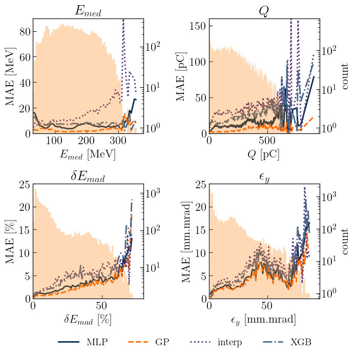
Figure 7: MAE for all the SM and all of the output with histograms representing the distribution of the output parameters of set2 in log scale

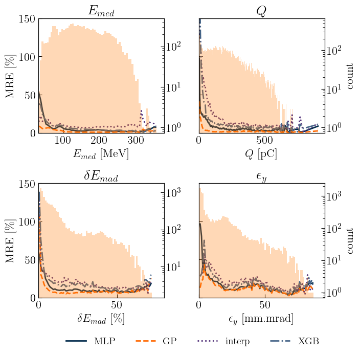
Figure 8: MRE for all the SM and all of the output with histograms representing the distribution of the output parameters of set2 in log scale.

We can see in Fig. 7,8 that the GP model is the best followed by the MLP. Even if GP have the best results MLP has the advantage of being less computationally expensive for a large amount of data. It also reveals that MRE increases dramatically for low output values, indicating that SM are less reliable at the lower end of the output intervals. Additionally, MAE tends to increase for the highest output values, since these values are underrepresented in the training data set as shown by the histograms depicting the distribution of the output parameters of set2 in Fig. 7,8.

In Fig. 9, the prediction of each SM is represented in a 2D subspace of $c_{N_{2}}$ and $p_{1}$. The projection are made for the input laser parameters fixed to $a_{0}=1.43$ and $x_{off}=-265\,\mu$m. One shoud notice that a complete set of projection can be generated in a few seconds on a laptop for a complete scan of $a_{0}$ and $x_{off}$ or other target parameters for more complex studies.

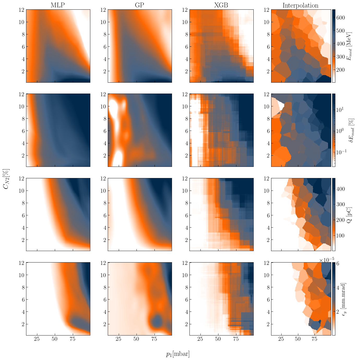
Figure 9: Surrogate LPI models prediction for all of the output in a 2D subspace of $p_{1}$ and $c_{N2}$ for $a_{0}=1.43$ and $x_{off}=-265\,\mu m$. Other snapshot of 2D subspace can be generated using python notebook available on the online repository[22]

V.2 Optimisation with the surrogate models

We have used the MLP model in the following analysis because it outperforms the XGB and interpolation methods, and works much faster than the GP when predicting large amounts of data. This is explained by the computational complexity of the GP and MLP methods which is $n^{3}$ [31] and $n\times d\times h$ [32], respectively. With $n$ the number of tested points, $d$ the input dimension of the MLP and $h$ the total number of neurons.

V.2.1 Optimum LPI working point stability

Using the MLP model, we looked for optimized working points. These points can be determined by several methods. The simplest approach is to generate a large number of data points using a continuous uniform distribution of 4D input parameters. The range of the input is kept within the boundaries of Tab. 1. From this dataset, our model can then be used to select beams with the desired characteristics. Selection is performed using the following filter: $\tilde{F}=\{E_{med}\in[195,205]\,$MeV, $\delta E_{mad}<5\,$%, $Q\in[25,35]\,$pC$\}$. We generated $5\,$million random configurations using a uniform distribution. From these $5\,$million configurations $2700$ were selected by filter $\tilde{F}$.

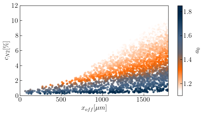
Figure 10: 2D subspace of $x_{off}$ and $c_{N2}$ of the input parameters for the configurations selected by filter $F$ with $a_{0}$ as a color scale.

We can see in Fig. 10, for each value of $x_{off}$, $c_{N2}$ logically decreases with $a_{0}$ since the target charge is fixed in the filter. If the laser energy is lower, the charge can be maintained at a certain level by increasing the doping rate as explained in [1]: not only the number of injected electrons can be increased but also increasing the self-focusing helps reaching a threshold value for $a_{0}$.

One interesting aspect to examine with this method is the stability across a target working point. Since the 5 million points were generated using a uniform distribution, each region of the 4D input space contains roughly the same number of points. Using the filter $\tilde{F}$ removes points of the input space which do not fulfil the condition $\tilde{F}$. Thus we consider that the region with the highest density of remaining points in the input space is the best, since it is the most stable.

In Fig. 11 we present stability maps as projections in 2D sub-spaces, showing the density of points $\eta_{stab}$ present in the input space of filter $\tilde{F_{1}}$, the density is represented with the colours scale. These stability maps can be used to guide the search for ideal electron beams. From this analysis, we identified that the most stable region within filter $\tilde{F_{1}}$ is centred around the following point: $a_{0}=1.12$, $c_{N_{2}}=9.2\,$%, $x_{off}=1.8\,$mm, $p_{1}=50\,$mbar.

V.2.2 Bayesian optimisation

Another method to find optimal working points is to use Bayesian optimisation on the surrogate models. We can employ either single-objective Bayesian optimisation or multi-objective Bayesian optimisation (MOBO). For single-objective optimisation, we used the following function: $\tilde{F}_{2}=\frac{\sqrt{Q}E_{med}}{\delta E_{mad}}$ [13], the Bayesian optimisation aimed to maximise this function. The optimisation consisted in one hundred steps with $20$ random evaluations. Out of the $120\,$points from the Bayesian optimisation, $64$ met or exceeded $95\,$% of the maximum of the objective function. PIC simulations were conducted for these $64$ configurations, resulting in beams with an average charge of $47\pm 4\,$pC, an average median energy of $266\pm 3\,$MeV, and an average energy spread of $5\pm 0.3\,\%$. In comparison the MLP model finds an average charge of $46\pm 4\,$pC, energy of $265\pm 2\,$MeV and energy spread of $2.3\pm 0.1\,\%$.

The MOBO aims at optimising simultaneously the elements of the following vector $\tilde{G}=(\delta E_{mad}(x),|E_{med}(x)-E_{0}|,Q(x))$ where $x$ is the 4D input vector. Our goal here is to maximise charge and minimise energy spread for a given median energy. We tried three MOBO search with the vector $\tilde{G}$ for three different central median energies $150$, $200$ and $250\,$MeV within a $\pm 10\,$MeV. Each MOBO consisted in $80\,$steps with $10$ random evaluation and $10$ evaluation for each step. This MOBO search resulted in Pareto fronts, which are illustrated in Fig. 12.

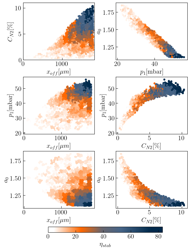
Figure 11: Stability map: Projection in the 2D sub-spaces of the configurations selected by filter $\tilde{F}_{1}$ with $\eta_{stab}$ as a color scale. These maps allow us to see the location of the most stable regions.

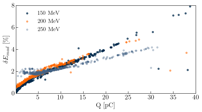
Figure 12: Scatter plot showing the result of MOBO search for 3 different energies $150,200$ and $250\,$MeV within a $\pm 10\,$MeV

We can see here a clear trade off between charge and energy spread. These solutions correspond to Pareto-optima [33] as we cannot improve one of the objective without deteriorating the other.

These three approaches permit to find target working points for the LPI. However we want to emphasise that the first one with filter $\tilde{F}$ is the most mature one because this allows us to find not only the beams of interest but also the most stable LPI configurations. This approach however requires to generate a large amount of data which is not a problem with the MLP model contrary to PIC simulations.

VI Conclusion and perspective

In conclusion, our in-depth numerical study focused on applying machine learning in the context, of a laser plasma injector optimisation design. It demonstrates that a surrogate model approach is relevant and efficient for beam optimisation and stability. We successfully constructed models that exhibit high performance in predicting electron beam parameters.

We emphasised the importance of data distribution in achieving accurate results with SM. Our analysis has shown that SM’s $R^{2}$ score converges rapidly towards $1$ if trained on sufficiently uniform data sets. This capability enabled us to effectively use the surrogate models to identify optimal working points for the design of LPI electron sources.

Furthermore, SM provides a comprehensive view of potential LPI beam parameters, facilitating the identification of stable operational regions and can drive the development of plasma target for higher repetition rate laser-plasma accelerator with limited laser intensity. These models are straightforward to implement and can be continuously refined by incorporating new simulation data.

However, we identified certain limitations of the surrogate models. They tend to under perform in regions where data points are sparse and exhibit poorer performance at the lower end of the output range. A potential improvement could be to add new simulations data in those regions and train our model on a larger interval of the output space than the test region.

Our study highlighted the ability of MLP and GP to generalise well and achieve the highest predictive performance among the ML methods considered.

This promising results shows that these methods could eventually be used with experimental data of the LPI or an hybrid version between experimental and simulation data since the time necessary to gather a large amount of experimental data is much shorter than PIC simulations. Such models could be implemented by using a multi-fidelity approach as in [34], more weight would be added to experimental data in comparison to simulations.

The next step is to create reverse SM to go from the output space to the input space. This task is numerically challenging since the 4 output parameters are not independent and the existence and unicity of the solution is not guaranteed. This is however a key step because it will help to properly design stable and efficient LPI. This would be a tool to introduce efficient feed back loop for LPI beam stabilisation.

VII Data Availability Statement

The features data and models that support the findings of this study are available online [22]. Raw PIC simulations data are available from the corresponding author upon reasonable request.

Appendix A Output electron beam parameters evaluation

The electron beam features are retrieved using a postprocessing script based on APtools python code [35] for the last time step corresponding to the end of the electron plasma density longitudinal profile. The figure Fig. 13 shows an example of median energy $E_{med}$, median absolute deviation $E_{mad}$ and charge corresponding to the integration of the electron beam energy distribution from the minimum energy tracked in the PIC code to the maximum energy.

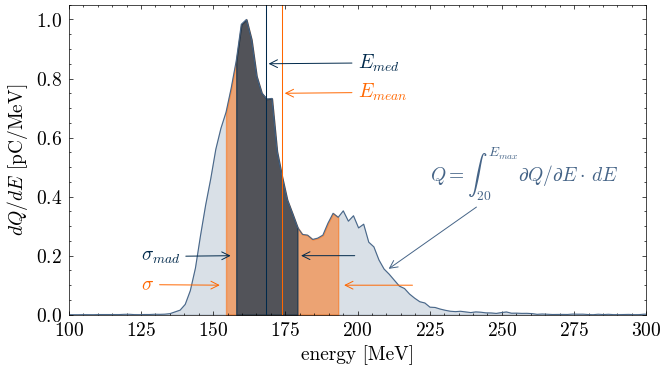
Figure 13: electron beam statistical features processed from the energy distribution

Only the trackParticles SMILEI openPMD output are used to post process electron beam features.

Appendix B Training surrogate model construction resources requirement

The training of the LPI surrogate models, as the number of input and output is limited, was done using a standard I7 Intel cpu.

The SM training time and computing time to generate $10^{5}$ LPI configurations are summarised in the following table tab. 4.

	training time [s]	$10^{5}$ configuration computing time [s]
MLP	300	4
GP	120	40
XGB	13	0.34

Table 4: Training time and computing for each type of method used to build the LPI model using I7 Intel cpu.

References

- [1] P. Drobniak, E. Baynard, C. Bruni, K. Cassou, C. Guyot, G. Kane, S. Kazamias, V. Kubytskyi, N. Lericheux, B. Lucas, M. Pittman, F. Massimo, A. Beck, A. Specka, P. Nghiem, and D. Minenna. Random scan optimization of a laser-plasma electron injector based on fast particle-in-cell simulations. Phys. Rev. Accel. Beams, 26:091302, Sep 2023.
- [2] Toshiki Tajima and John M Dawson. Laser electron accelerator. Physical review letters, 43(4):267, 1979.
- [3] Eric Esarey, Carl B Schroeder, and Wim P Leemans. Physics of laser-driven plasma-based electron accelerators. Reviews of modern physics, 81(3):1229, 2009.
- [4] Jérôme Faure, Yannick Glinec, A Pukhov, S Kiselev, S Gordienko, E Lefebvre, J-P Rousseau, F Burgy, and Victor Malka. A laser–plasma accelerator producing monoenergetic electron beams. Nature, 431(7008):541–544, 2004.
- [5] M-C Vozenin, Jolyon H Hendry, and CL Limoli. Biological benefits of ultra-high dose rate flash radiotherapy: sleeping beauty awoken. Clinical oncology, 31(7):407–415, 2019.
- [6] Wolfram Helml, Ivanka Grguraš, Pavle N Juranić, Stefan Düsterer, Tommaso Mazza, Andreas R Maier, Nick Hartmann, Markus Ilchen, Gregor Hartmann, Luc Patthey, et al. Ultrashort free-electron laser x-ray pulses. Applied Sciences, 7(9):915, 2017.
- [7] AJ Gonsalves, K Nakamura, J Daniels, C Benedetti, C Pieronek, TCH De Raadt, S Steinke, JH Bin, SS Bulanov, J Van Tilborg, et al. Petawatt laser guiding and electron beam acceleration to 8 gev in a laser-heated capillary discharge waveguide. Physical review letters, 122(8):084801, 2019.
- [8] JP Couperus, R Pausch, A Köhler, O Zarini, JM Krämer, M Garten, A Huebl, R Gebhardt, U Helbig, S Bock, et al. Demonstration of a beam loaded nanocoulomb-class laser wakefield accelerator. Nature communications, 8(1):487, 2017.
- [9] LT Ke, K Feng, WT Wang, ZY Qin, CH Yu, Y Wu, Y Chen, R Qi, ZJ Zhang, Y Xu, et al. Near-gev electron beams at a few per-mille level from a laser wakefield accelerator via density-tailored plasma. Physical review letters, 126(21):214801, 2021.
- [10] JY Mao, LM Chen, K Huang, Y Ma, JR Zhao, DZ Li, WC Yan, JL Ma, M Aeschlimann, ZY Wei, et al. Highly collimated monoenergetic target-surface electron acceleration in near-critical-density plasmas. Applied Physics Letters, 106(13), 2015.
- [11] Charles K Birdsall and A Bruce Langdon. Plasma physics via computer simulation. CRC press, 2018.
- [12] Andreas Döpp, Christoph Eberle, Sunny Howard, Faran Irshad, Jinpu Lin, and Matthew Streeter. Data-driven science and machine learning methods in laser–plasma physics. High Power Laser Science and Engineering, 11:e55, 2023.
- [13] Sören Jalas, Manuel Kirchen, Philipp Messner, Paul Winkler, Lars Hübner, Julian Dirkwinkel, Matthias Schnepp, Remi Lehe, and Andreas R Maier. Bayesian optimization of a laser-plasma accelerator. Physical review letters, 126(10):104801, 2021.
- [14] Faran Irshad, Christoph Eberle, FM Foerster, K v Grafenstein, F Haberstroh, E Travac, N Weisse, Stefan Karsch, and Andreas Döpp. Pareto optimization of a laser wakefield accelerator. arXiv preprint arXiv:2303.15825, 2023.
- [15] M Chen, E Esarey, CB Schroeder, CGR Geddes, and WP Leemans. Theory of ionization-induced trapping in laser-plasma accelerators. Physics of Plasmas, 19(3), 2012.
- [16] G Golovin, Shouyuan Chen, N Powers, Cheng Liu, Sudeep Banerjee, J Zhang, M Zeng, Z Sheng, and D Umstadter. Tunable monoenergetic electron beams from independently controllable laser-wakefield acceleration and injection. Physical Review Special Topics-Accelerators and Beams, 18(1):011301, 2015.
- [17] Julien Derouillat, Arnaud Beck, Frédéric Pérez, Tommaso Vinci, M Chiaramello, Anna Grassi, M Flé, Guillaume Bouchard, I Plotnikov, Nicolas Aunai, et al. Smilei: A collaborative, open-source, multi-purpose particle-in-cell code for plasma simulation. Computer Physics Communications, 222:351–373, 2018.
- [18] F Massimo, A Beck, J Derouillat, M Grech, M Lobet, F Pérez, I Zemzemi, and A Specka. Efficient start-to-end 3d envelope modeling for two-stage laser wakefield acceleration experiments. Plasma Physics and Controlled Fusion, 61(12):124001, oct 2019.
- [19] F. Massimo, I. Zemzemi, A. Beck, J. Derouillat, and A. Specka. Efficient cylindrical envelope modeling for laser wakefield acceleration. Journal of Physics: Conference Series, 1596(1):012055, jul 2020.
- [20] F. Massimo, A. Beck, J. Derouillat, I. Zemzemi, and A. Specka. Numerical modeling of laser tunneling ionization in particle-in-cell codes with a laser envelope model. Physical Review E, 102(3):033204, September 2020. tex.ids= massimo:2020 arXiv: 2006.04433 publisher: American Physical Society.
- [21] Genci center for high performance computing. https://www.genci.fr/en. Accessed: 2010-09-30.
- [22] LPA PIC simulations Data: Lpi surrogate models. https://gitlab.in2p3.fr/lpa-pic-simulations-data/lpisurrogate, 2024.
- [23] P. Drobniak, E. Baynard, K. Cassou, D. Douillet, J. Demailly, A. Gonnin, G. Iaquaniello, G. Kane, S. Kazamias, N. Lericheux, B. Lucas, B. Mercier, Y. Peinaud, and M. Pittman. Two-chamber gas target for laser-plasma accelerator electron source, 2023.
- [24] Wei Lu, M Tzoufras, C Joshi, FS Tsung, WB Mori, J Vieira, RA Fonseca, and LO Silva. Generating multi-gev electron bunches using single stage laser wakefield acceleration in a 3d nonlinear regime. arXiv preprint physics/0612227, 2006.
- [25] Tom Dietterich. Overfitting and undercomputing in machine learning. ACM computing surveys (CSUR), 27(3):326–327, 1995.
- [26] Martín Abadi, Paul Barham, Jianmin Chen, Zhifeng Chen, Andy Davis, Jeffrey Dean, Matthieu Devin, Sanjay Ghemawat, Geoffrey Irving, Michael Isard, et al. TensorFlow: a system for Large-Scale machine learning. In 12th USENIX symposium on operating systems design and implementation (OSDI 16), pages 265–283, 2016.
- [27] Kaiming He, Xiangyu Zhang, Shaoqing Ren, and Jian Sun. Delving deep into rectifiers: Surpassing human-level performance on imagenet classification. In Proceedings of the IEEE international conference on computer vision, pages 1026–1034, 2015.
- [28] Payam Refaeilzadeh, Lei Tang, and Huan Liu. Cross-validation. Encyclopedia of database systems, pages 532–538, 2009.
- [29] Tianqi Chen and Carlos Guestrin. Xgboost: A scalable tree boosting system. In Proceedings of the 22nd acm sigkdd international conference on knowledge discovery and data mining, pages 785–794, 2016.
- [30] GPy: A gaussian process framework in Python. http://github.com/SheffieldML/GPy, 2014.
- [31] Christopher Williams and Carl Edward Rasmussen. Gaussian processes for machine learning, volume 2. MIT press Cambridge MA, 2006.
- [32] Ian Goodfellow, Yoshua Bengio, and Aaron Courville. Deep Learning. MIT Press, 2016. http://www.deeplearningbook.org.
- [33] Soeren Jalas, M Kirchen, C Braun, T Eichner, JB Gonzalez, Lars Hübner, T Hülsenbusch, P Messner, G Palmer, M Schnepp, et al. Tuning curves for a laser-plasma accelerator. Physical Review Accelerators and Beams, 26(7):071302, 2023.
- [34] Faran Irshad, Stefan Karsch, and Andreas Döpp. Multi-objective and multi-fidelity bayesian optimization of laser-plasma acceleration. Physical Review Research, 5(1):013063, 2023.
- [35] APtools: Accelerator physics tools in Python. https://github.com/AngelFP/APtools, 2024.